The Economics of Social Data

Abstract

A data intermediary acquires signals from individual consumers regarding their preferences. The intermediary resells the information in a product market wherein firms and consumers tailor their choices to the demand data. The social dimension of the individual data—whereby a consumer’s data are predictive of others’ behavior—generates a data externality that can reduce the intermediary’s cost of acquiring the information. The intermediary optimally preserves the privacy of consumers’ identities if and only if doing so increases social surplus. This policy enables the intermediary to capture the total value of the information as the number of consumers becomes large.

Keywords: social data; personal information; consumer privacy; privacy paradox; data intermediaries; data externality; data policy; data rights; collaborative filtering.

JEL Classification: D44, D82, D83.

1 Introduction

Individual and Social Data

The rise of large digital platforms—such as Facebook, Google, and Amazon in the US and JD, Tencent and Alibaba in China—has led to the unprecedented collection and commercial use of individual data. The steadily increasing user bases of these platforms generate massive amounts of data about individual consumers, including their preferences, locations, friends, and political views. In turn, many of the services provided by large Internet platforms rely critically on these data. The availability of individual-level data permits refined search results, personalized product recommendations, informative ratings, timely traffic data, and targeted advertisements.

The recent disclosures on the use and misuse of social data by digital platforms have prompted regulators to limit the largely unsupervised use of individual data by these companies. As a result, nearly all proposed and enacted regulation to date aims to ensure that consumers retain control over their data. However, the digital privacy paradox (e.g., atct17) indicates that even small monetary incentives may lead individuals to relinquish their private data. The low cost of acquiring private data–seemingly at odds with consumers’ stated preferences over their privacy– drives the appetite of platforms to gather information and may undermine the efficacy of regulation.

This article suggests a unified explanation for the digital privacy paradox and the selective use of data for price and product choices. A key observation is that individual data are actually social data: data captured from an individual user are informative not only about that user but also about other users with similar characteristics or behaviors. The social dimension of the data generates a data externality, the sign and magnitude of which depend on the structure of the data and on the use of the gained information.

Many digital platforms use social data to increase the value provided by their services. Google search results, for example, are informed by the choices of previous users. Indeed, the search engine is only successful because it mediates information among many consumers. Likewise, Amazon uses data collected from other consumers to curate a “recommended for you” list of products and explicitly suggests goods that are “frequently bought together.” Finally, YouTube and Waze tailor their suggestions of videos and traffic directions to each user’s preferences, as estimated by combining network data and individual data. However, social data also facilitates surplus extraction, e.g., individual shopping data convey information about the willingness to pay of consumers with similar purchase histories.

We analyze three critical aspects of the economics of social data. First, we consider how the collection and transmission of individual data change the terms of trade among consumers, firms (e.g., advertisers), and data intermediaries (e.g., large Internet platforms that sell targeted advertising space). Second, we examine how the social dimension of the data magnifies the value of individual data for platforms and facilitates the acquisition of large datasets. Third, we analyze how data intermediaries with market power manipulate the trade-offs induced by social data through the aggregation and the precision of the information that they provide about consumers.

A Model of Data Intermediation

We develop a framework to evaluate the flow and allocation of individual data in the presence of data externalities. Our model focuses on three types of economic agents: consumers, firms, and data intermediaries. These agents interact in two distinct but linked markets: a data market and a product market.

In the product market, each consumer (she) determines the quantity that she wishes to purchase, and a single producer (he) sets the unit price at which he offers a product to the consumers. Initially, each consumer has private information about her willingness to pay for the firm’s product. This information consists of a signal with two additive components: a  fundamental component and a noise component. The fundamental component represents her willingness to pay, and the noise component reflects that her initial information might be imperfect. Both components can be correlated across consumers: in practice, different consumers’ preferences can exhibit common traits, and consumers might undergo similar experiences that induce correlation in their errors.

In the data market, a monopolist intermediary acquires demand information from the individual consumers in exchange for a monetary payment. The intermediary then chooses how much information to share with the other consumers and how much information to sell to the producer. Sharing data with consumers allows them to tailor their demand to their true preferences. Sharing data with the producer enables more tailored and possibly personalized prices.

We introduce a rich model for the structure of individual data, which allows for correlation in the fundamentals as well as in the noise terms across the individuals. We view this richness in the data structure as the defining element of data in digital platforms. In contrast, we adopt a more specific model for product market interaction whereby a monopolist seller charges linear prices for variable quantity. However, our main insights apply to any product market where (a) data sharing teaches consumers about their preferences, and (b) a firm seeks to extract the consumers’ surplus.

The Value of Social Data

Collecting data from multiple consumers helps any market participant to filter the individual signals. This process can occur through two channels. First, in a market where the noise terms are largely idiosyncratic, a large sample size filters out errors and identifies any common fundamentals. Second, in a market with largely idiosyncratic fundamentals, many observations filter out demand shocks and identify common noise terms, thereby estimating individual fundamentals by differencing (Proposition 1).

However, the choice by each consumer to share her data with the intermediary is guided only by her private benefits and costs, not by the information gains she generates with her actions. Thus, the intermediary must compensate each individual consumer only to the extent that the disclosed information affects her own welfare on the margin. Critically, the platform does not have to compensate the individual consumer for any changes in her welfare caused by the information deduced from other consumers’ signals.

Therefore, social data drive a wedge between the socially efficient and profitable uses of information. First, the cost of acquiring individual data can be substantially less than the value of the information to the platform. Second, although many uses of consumer information exhibit positive externalities, very little prevents the platform from trading data for profitable uses that are in fact harmful to consumers (Proposition 2).

More generally, the data externality can induce too much or too little trade in data. Indeed, the condition for data intermediation to yield positive profits is qualitatively different from the condition for intermediation to yield social welfare gains. In particular, the intermediary obtains positive profits when a large number of consumers exhibit a strong degree of correlation in their preferences: this allows the intermediary to acquire the consumers’ data in exchange for minimal compensation. On the other hand, welfare improvements depend on how much additional information each consumer can obtain about her own preferences from the other consumers’ signals. Therefore, when many consumers have strongly correlated preferences and very precise signals, data sharing is detrimental to welfare but profitable to the intermediary. Conversely, there are data structures (e.g., ones with independent fundamentals and strongly correlated error terms) for which data sharing is beneficial to consumers but unprofitable for the data intermediary.

Equilibrium Data-Sharing Policies

A natural question is then whether the data market imposes any limitations at all on equilibrium information sharing. To shed light on this issue, we consider the choice of whether to reveal the consumers’ identities to the producer or to collect anonymous data. When consumers are homogeneous ex ante, we show that the intermediary collects anonymous data if and only if the transmission of identity data reduces total surplus. Therefore, even if the data transmission may be socially detrimental, the optimal choice of data anonymization is socially efficient (Proposition 3).

In our model of linear price discrimination, collecting anonymous data amounts to selling aggregate, market-level information to the producer. With this choice, the intermediary does not enable the producer to set personalized prices: the data are transmitted but disconnected from the users’ personal profiles. In other words, the role of social data provides a more nuanced ability to determine the modality of information acquisition and use.

Under anonymized data intermediation, the gap between the social value of the data and the price of the data widens when the number of consumers increases. In particular, as the sources of data multiply, the contribution of each individual consumer to the aggregate information shrinks, which drives down the individual payments to consumers, and possibly the total payment as well (Proposition 5).

We develop a general anonymization result (Proposition 8) and extend the model in several directions. We first introduce consumer heterogeneity by considering multiple groups of consumers. We find that the intermediary aggregates the data at least to the level of the coarsest partition of homogeneous consumers, although further aggregation is profitable when the number of consumers is small. The resulting group pricing—discriminatory pricing based on observable characteristics, such as location—has welfare consequences between those of complete privacy and those of price personalization (Proposition 9).

We then consider a model in which the producer can choose prices and product characteristics to match an additional horizontal (taste) dimension of the consumers’ preferences. The resulting data policy then aggregates the vertical dimension but not the horizontal dimension, thereby enabling the producer to offer personalized product recommendations but not personalized prices (Proposition 10). Finally, in the Online Appendix, we explore the data intermediary’s ability to offer privacy guarantees by collecting less than perfect information about the consumers’ signals.

Implications and Applications

There exist a wide variety of data intermediaries and associated business models. The point of our article is not to try to match any specific business model but rather to speak to the general principles that seem to be in effect in many markets. In particular, our model assumes that each consumer is compensated directly with a monetary transfer for her individual data. There exist a few concrete examples of such transactions (e.g., Nielsen offers monetary rewards to consumers for access to their browsing and purchasing data). However, most data intermediaries compensate their users via the quality of the services they offer, e.g., social networks, search, mail, video. These services are nominally free, but in practice (through more or less transparent terms and conditions) they are fueled by the data generated by their users.

Likewise, digital platforms occasionally transfer consumers’ data to merchants for a fee. Much more often, however, they monetize their data by selling access to targeted advertising campaigns—see the report by the cma20. This enables the merchants to reap the value of information, by conditioning their messages and their prices on the consumers’ preferences, without directly observing their data. These transactions amount to indirect sales of information, as discussed in bebo19.

Our model’s predictions for the nature of the externality, for the equilibrium allocation of data, and for its welfare properties then depend on how targeted advertising affects total surplus in any given market. Specifically, if advertising generates value by matching of buyers and sellers, as in bebo11, our model would predict the intermediation of individual-level information through very detailed targeting categories. If, instead, targeted advertisements facilitate inefficient price discrimination, the model would predict coarser targeting categories that induce market-level or group-level pricing.

Related Literature

This article contributes to the growing literature on data markets recently surveyed in bebo19. In particular, the role of data externalities in the socially excessive diffusion of personal data has been a central concern in chjk19 and ammo21, both considering a model with many buyers and one firm that acts as an integrated data intermediary and seller.

chjk19 introduce information externalities into a model of monopoly pricing with unit demand. Each consumer is described by two independent random variables: her willingness to pay for the monopolist’s service and her sensitivity to a loss of privacy. The purchase of the service by the consumer requires the transmission of personal data. From the collected data, the seller gains additional revenue, depending on the proportion of units sold and the volume of data collected. The total nuisance cost paid by each consumer depends on the total number of consumers sharing their personal data. Thus, the optimal pricing policy of the monopolist yields excessive loss of privacy, relative to the social welfare maximizing policy.

ammo21 also analyze data acquisition in the presence of information externalities. As in chjk19, they consider a model with many consumers and a single data-acquiring firm. Like the current analysis, ammo21 propose an explicit statistical model for their data; the model allows the authors to assess the loss of privacy for the consumer and the gains in prediction accuracy for the firm. Their analysis then pursues a different, and largely complementary, direction from ours. In particular, they analyze how consumers with heterogeneous privacy concerns trade information with a data platform and derive conditions under which the equilibrium allocation of information is (in)efficient.

In contrast to these two important contributions, we explicitly introduce a data intermediary with objectives distinct from either the consumers or the seller. We consider rich data structures for fundamentals and noise terms that capture the wide range of social data on digital platforms. This allows us to endogenize privacy concerns and to quantify the downstream welfare impact of data intermediation. In addition, we can investigate when and how privacy can be partially or fully preserved through aggregation, anonymization, and noise. Thus, we augment the analysis in the above contributions with additional insights regarding data flows and data intermediation. In particular, we show that the data externality can have a positive or a negative impact on consumer and social surplus depending on the data structure. In consequence, a monopolist intermediary can induce either too little or too much information sharing in equilibrium.

actw16 survey the literature on the economics of privacy in great detail. An early and influential article is tayl04, who analyzes the sales of consumer purchase histories without data externalities. More recently, clpr16 investigate how privacy policies affect user and advertiser behavior in a simple model of targeted advertising. The low level of compensation that users command for their personal data is discussed in agjl18, who propose sources of countervailing market power, and in a growing body of empirical work. In particular, tang19 uses large-scale field experiments to estimate the value that online borrowers assign to several pieces of personal data. lin19 separates intrinsic and instrumental preferences for privacy through a lab experiment that also uncovers data externalities.

fagm20 provide a digital privacy model in which data collection improves the service provided to consumers. However, as the collected data can also leak to third parties and thus impose privacy costs, an optimal digital privacy policy must be established. Similarly, julr20 analyze the equilibrium privacy policy of websites that monetize information collected from users by charging third parties for targeted access. grad17 considers a network game in which the level of beneficial information sharing among the players is limited by the possibility of leakage and a decrease in informational interdependence. allv19 study a model of personalized pricing with disclosure by an informed consumer, and they analyze how different disclosure policies affect consumer surplus. ichi20aer studies both personalized pricing and product recommendations, and shows that a seller benefits from committing not to use the consumer’s information to set prices. Our result on optimal anonymization and market-level pricing has similar implications, but is entirely driven by the data externality that appears when multiple consumers are present.

Finally, lima20 investigate how data policies can provide incentives in principal-agent relationships. They emphasize the structure of individual data and how the substitutes or complements nature of individual signals determines the impact of data on incentives. ichi20 considers a single data intermediary and asks how complements or substitutes consumer signals affect the equilibrium price of the individual data.

2 Model

We consider an idealized trading environment with many consumers, a single intermediary in the data market, and a single producer in the product market.

2.1 Product Market

There are finitely many consumers, labeled $i=1,...,N$. In the product market, each consumer (she) chooses a quantity level $q_{i}$ to maximize her net utility given a unit price $p_{i}$ offered by the producer (he):

$$u_{i}\left(w_{i},q_{i},p_{i}\right)\triangleq w_{i}q_{i}-p_{i}q_{i}-\frac{1}{2}q_{i}^{2}.$$

Each consumer $i$ has a baseline willingness to pay for the product $w_{i}\in\mathbb{R}$.

The producer sets the unit price $p_{i}$ at which he offers his product to each consumer $i$. The producer has a linear production cost

$$c\left(q\right)\triangleq c\cdot q,\ \text{for some}\ \ c\geq 0.$$

The producer’s profits are given by

$$\pi\left(p_{i},q_{i}\right)\triangleq\sum_{i}\left(p_{i}-c\right)q_{i}.$$

2.2 Data Environment

The vector of willingness to pay, $w=\left(...,w_{i},...\right)\in\mathbb{R}^{N}$, is distributed according to a joint distribution $F_{w}$:

$$w\sim F_{w}.$$ (1)

Initially, each consumer may have only imperfect information about her willingness to pay. In particular, consumer $i$ observes a signal

$$s_{i}\triangleq w_{i}+\sigma\cdot e_{i}\text{,}$$ (2)

where $\sigma>0$ and $e_{i}$ is consumer $i$’s error term. The error terms $e=\left(...,e_{i},...\right)\in\mathbb{R}^{N}$ are independent of the willingness to pay $w$, and they are distributed according to a joint distribution $F_{e}$:

$$e\sim F_{e}.$$ (3)

We denote by $S$ the information structure generated by the complete vector of consumer signals $s=\left(...,s_{i},...\right)\in\mathbb{R}^{N}$. We allow for arbitrary distributions of fundamentals $w$ and errors $e$, and hence arbitrary correlation structures across consumers, under the restriction that the $\left(F_{w},F_{e}\right)$ are symmetric across individuals. We view the richness in the data structure as represented by (1) and (3) as the defining feature of social data in the digital economy. In particular, the noise in the signal $s_{i}$ of each individual given by (2) reflects the importance of social learning as enabled by recommenders, rating and search engines.

Without loss of generality we assume that (i) each individual willingness to pay $w_{i}$ has mean $\mu$ and variance $1$; (ii) individual errors $e_{i}$ have mean $0$ and variance $1$ (which is scaled by the parameter $\sigma$).

The producer knows the structure of demand and thus the common prior distribution of consumers’ willingness to pay. However, absent any additional information, the producer does not know the realized willingness to pay $w_{i}$ of any consumer (nor her signal $s_{i}$) prior to setting prices. This data environment has two important features. First, any demand information beyond the common prior comes from the signals of the individual consumers. Second, with any amount of noise in the signals (i.e., if $\sigma>0$), each consumer can learn more about her own demand from the signals of the other consumers.

The following leading examples illustrate two ways in which data sharing can help each consumer learn more about her individual willingness to pay. In, Example 1 a new product has a common value that consumers are imperfectly informed about.

Example 1 (Common Preferences)

Fundamentals $w_{i}$ are perfectly correlated and errors $e_{i}$ are independent: $s_{i}=w+\sigma\cdot e_{i}$.

In this case, data sharing helps to filter out the idiosyncratic error terms: as $N$ becomes large, the average signal across all consumers identifies the common willingness to pay.

In Example 2, individual consumers have independent values for a new therapy but are exposed to a common health shock.

Example 2 (Common Experience)

Errors $e_{i}$ are perfectly correlated, and fundamentals $w_{i}$ are independent: $s_{i}=w_{i}+\sigma\cdot e.$

Under this structure, the average signal identifies the common error component $e$ as $N$ becomes large. All market participants can then precisely estimate each $w_{i}$ from the difference between individual and average signal.

As we shall see, information sharing enables learning in both examples. However, the actions of consumers $-i\$impact the surplus of consumer $i$ quite differently in the two cases, which has implications for the equilibrium price of data. More generally, the data structure will determine how to separate the individual and the aggregate information.

2.3 Data Market

The data market is run by a single data intermediary (it). As a monopolist market maker, the data intermediary decides how to collect the available information $\left(s_{i}\right)$ from each consumer and how to share it with the other consumers and the producer. Thus, the data intermediary faces both an information design problem and an information pricing problem.

We consider bilateral contracts between the individual consumers and the intermediary and between the producer and the intermediary. The data intermediary offers these bilateral contracts ex ante, i.e., before the realization of any demand shocks. Each bilateral contract defines a data policy and a data price.

The data contract with consumer $i$ specifies a data inflow policy $X_{i}$ and a fee $m_{i}\in\mathbb{R}$ paid to the consumer. The data inflow policy describes how each signal $s_{i}\$enters the database of the intermediary. We restrict attention to the following two policies: (i) the complete (identity-revealing) data policy $X=S$, where the intermediary collects each consumer’s signal $s_{i}$; and (ii) the anonymized data policy $X=A$, where the intermediary collects individual signals without identifying information. We model the anonymized data policy as

$$A:S\rightarrow\delta\left(S\right)\text{,}$$

for a random permutation of the consumers’ indices $i\rightarrow\delta\left(i\right)$. In both cases, as discussed in Section 2 below, there are no further incentive constraints, i.e., consumers transmit their information truthfully.

In our product market model, where the consumer’s demand is linear in her signal, the anonymized data policy $A$ is equivalent to an aggregate data policy that conveys information about the average willingness to pay. Intuitively, the anonymized data policy prevents the producer from matching signals to consumers, i.e., from profitably charging personalized prices. In Section Appendix B, we enrich the intermediary’s strategy space by allowing for data policies that collect partial information about the consumers’ signals.

A data contract with the producer specifies a data outflow policy $Y$ and a fee $m_{0}\in\mathbb{R}$ paid by the producer. The data outflow policy determines how each consumer’s collected signal is transmitted to the producer and to other consumers. In particular, letting $X$ denote the intermediary’s realized data inflow, a data outflow policy $Y=\left(Y_{0},Y_{1},\dots Y_{N}\right)$ describes how the collected data are released to the seller,

$$Y_{0}:X\rightarrow\Delta(\mathbb{R}^{N}),$$

and to each consumer,

$$Y_{i}:X\rightarrow\Delta(\mathbb{R}^{N}).$$

Sharing data with other consumers is a critical design element because doing so allows each consumer to adjust her quantity demanded at any price. Therefore, the information received by consumers also impacts the  producer’s willingness to pay for the intermediary’s data.

The data intermediary maximizes the net revenue

$$R\triangleq m_{0}-\sum\nolimits_{i=1}^{N}m_{i}.$$ (4)

2.4 Equilibrium and Timing

The game proceeds sequentially. First, the terms of trade on the data market and then the terms of trade on the product market are established. The timing of the game is as follows:

1. The data intermediary offers a data inflow policy $\left(m_{i},X_{i}\right)$ to each consumer $i$. Consumers simultaneously accept or reject the intermediary’s offer.

2. The data intermediary offers a data outflow policy $\left(m_{0},Y\right)$ to the producer, based on the (known) number of consumers who have accepted. The producer accepts or rejects the offer.

3. Consumers’ signals $s$ are realized, and the information flows $\left(x,y\right)$ are transmitted according to the terms of the data policies.

4. The producer sets a unit price $p_{i}$ for each consumer $i$ who makes a purchase decision $q_{i}$, given her available information about $w_{i}$.

We analyze the Perfect Bayesian Equilibria of the game. Under the timing described above, information is imperfect but symmetric at the contracting stage. Furthermore, when the consumer receives the intermediary’s offer, she must anticipate the intermediary’s choice of data outflow policy, which determines what data are shared with her, as well as with the producer. We denote by $a_{0},a_{i}\in\left\{0,1\right\}$ the participation decisions by the producer and by consumer $i$, respectively. A Perfect Bayesian Equilibrium is then a tuple of inflow and outflow data policies, data and product pricing policies, and participation decisions:

$$\left\{\left(X^{\ast},Y^{\ast},m^{\ast}\right);~{}p^{\ast},q^{\ast};~{}a^{\ast}\right\},$$

where

$$a_{0}^{\ast}:X\times Y\times\mathbb{R\rightarrow}\left\{0,1\right\},~{}a_{i}^{\ast}:X_{i}\times\mathbb{R\rightarrow}\left\{0,1\right\},$$

such that (i) the producer maximizes his expected profits, (ii) the intermediary maximizes its expected revenue, and (iii) each consumer maximizes her net utility. In our baseline analysis, we focus on the best equilibrium for the data intermediary; in the best equilibrium, every consumer accepts the offer from the data intermediary. We discuss a unique implementation in Section 4.3.

Figure 1 summarizes the information and value flow in the data and product markets.

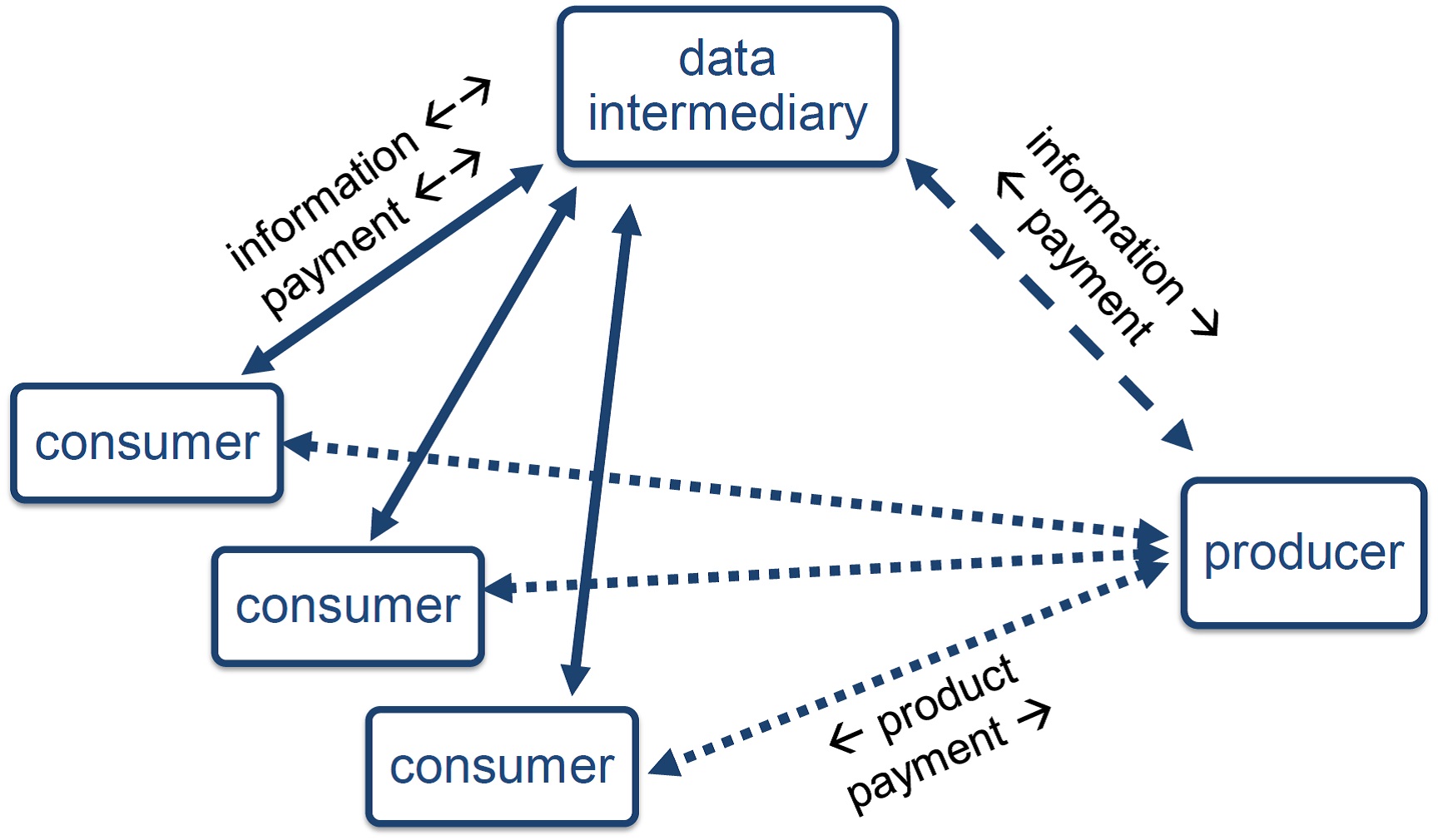
Figure 1: Data and Value Flows

Discussion of Model Features

Participation Constraints  The participation constraints of every consumer and of the producer are required to hold at the ex ante level. Thus, the consumers agree to the data policy before the realization of their signals. The choice of ex ante participation constraints captures the prevailing conditions under which users interact with large digital platforms. For instance, users of services on Amazon, Facebook, or Google typically establish an account and accept the “terms of service” before making any specific query or post. Through the lens of our model, the consumer requires a level of compensation that allows her to profitably share the information in expectation. Upon agreeing to participate, there are no further incentive compatibility constraints on the transmission of her information.

Lack of Commitment  As we mentioned above, targeted advertising is the primary source of revenue for digital platforms. Consequently, the data intermediary in our sequential game sells the consumers’ data only to the producer, and cannot commit to withholding any information from him. Similarly, the intermediary’s choice of data outflow policy occurs after consumers are enlisted but before their data are realized. This assumption captures the limited ability of a platform to write advertising contracts contingent on, say, the volume of activity taking place at any point in time.

Linear Price Discrimination  The producer in our baseline model uses the consumers’ data to charge a unit price to each consumer. Whether richer pricing instruments enable online merchants to implement more sophisticated forms of price discrimination is largely an empirical question. However, as we discuss in Section 5.1, the general anonymization result of Proposition 8 guides the intermediary’s optimal data policy even if the producer can extract more of the surplus generated through better information. Indeed, even in the case of perfect price discrimination, the presence of the data externality would continue to drive a gap between equilibrium and socially efficient allocation.

3 Value of Social Data

3.1 Data Sharing and Product Market

In our extensive form game, given the realized data inflow, the intermediary offers a data outflow policy to the producer. This policy specifies both the fee $m_{0}$ and the flow of information to all market participants, including the consumers. The data outflow policy thus determines both how well informed the producer is and how well informed his customers are.

Because the information is being sold to the producer, the intermediary will choose a data outflow policy that maximizes the producer’s profits, and then extracts the value of this information through the fee $m_{0}$. The intermediary’s choice of outflow policy is simplified considerably by the following result, which allows us to restrict attention to policies in which every consumer is weakly better informed than the producer.

Lemma 1 (Data Outflow Policy)

For any data inflow $X$, it is without loss of generality to consider data outflow policies where $Y_{0}(X)$ is measurable with respect to each $Y_{i}(X)$.

Interestingly, the result of Lemma 1 does not rely on the specific nature of the product market interaction. The key observation is that, if the producer were better informed, the prices charged would convey information to consumers about their own willingness to pay. The ensuing signaling incentives impose a cost on the producer because he will need to deviate from the prices that maximize his profits, holding fixed the consumers’ beliefs. The intermediary can then increase the producer’s profits (weakly) by revealing any information contained in the equilibrium prices directly to the consumers. Furthermore, this improvement is strict if, when the consumers receive this additional information, the producer modifies his choice of price.

Under the data outflow policies of Lemma 1, we can easily quantify the value of information for consumers and producers. The shared data help each consumer estimate her own willingness to pay. For the producer, the shared data enable a more informed pricing policy. In particular, given the realized data outflow $y\in Y$, the optimal pricing policy for the producer consists of a vector of (potentially personalized) prices $p_{i}^{\ast}$, thus resulting in a vector of individual quantities $q_{i}^{\ast}$ purchased. We denote the predicted value of consumer $i$’s willingness to pay, given the signals $\left(s_{i},y_{i}\right)$ by:

$$\widehat{w}_{i}\left(s_{i},y_{i}\right)\triangleq\mathbb{E}\left[w_{i}\mid s_{i},y_{i}\right].$$

The realized demand of consumer $i$ is given by

$$q_{i}\left(s_{i},y_{i},p\right)=\widehat{w}_{i}\left(s_{i},y_{i}\right)-p.$$

As $Y_{0}$ is (weakly) less informative than $Y_{i}$, the producer chooses the optimal price

$$p_{i}^{\ast}\left(y_{0}\right)=\frac{\mathbb{E}[\widehat{w}_{i}\left(s_{i},y_{i}\right)|Y_{0}]+c}{2}=\frac{\widehat{w}_{i}\left(y_{0}\right)+c}{2}\text{,}$$

which results in the equilibrium quantity:

$$q_{i}^{\ast}\left(s_{i},y_{i},y_{0}\right)\triangleq q_{i}\left(s_{i},y_{i},p_{i}^{\ast}\left(y_{0}\right)\right).$$

The ex ante expected profit of the producer from interacting with consumer $i$ is given by

$$\Pi_{i}\left(\left(S_{i},Y_{i}\right),Y_{0}\right)\triangleq\mathbb{E}\left[\pi\left(p_{i}^{\ast}\left(y_{0}\right),q_{i}^{\ast}\left(s_{i},y_{i},y_{0}\right)\right)\left|Y_{0}\right.\right]=\frac{1}{4}\mathbb{E}\left[(\widehat{w}_{i}\left(y_{0}\right)-c)^{2}\left|Y_{0}\right.\right].$$

The first argument in $\Pi_{i}\left(\cdot,\cdot\right)$ refers to consumer $i$’s information structure $\left(S_{i},Y_{i}\right)$ and the second argument refers to the producer’s information structure $Y_{0}$. Similarly, we denote the indirect utility of consumer $i$ as

$$U_{i}\left(\left(S_{i},Y_{i}\right),Y_{0}\right)\triangleq\mathbb{E}\left[u_{i}\left(w_{i},q_{i}^{\ast}\left(s_{i},y_{i},y_{0}\right),p_{i}^{\ast}\left(y_{0}\right)\right)\left|S_{i},Y_{i}\right.\right]=\frac{1}{2}\mathbb{E}\left[(\widehat{w}_{i}\left(s_{i},y_{i}\right)-p_{i}^{\ast}\left(y_{0}\right))^{2}\left|S_{i},Y_{i}\right.\right].$$

3.2 Welfare Effects of Data Sharing

The model with quadratic payoffs (regardless of the prior distribution of consumers’ willingness to pay) yields explicit expressions for the value of information for product market participants. In particular, because prices and quantities are linear functions of the posterior mean $\widehat{w}_{i}$, the ex ante average prices and quantities $\mathbb{E}\left[p^{\ast}\right]$ and $\mathbb{E}\left[q^{\ast}\right]$ are constant across all information structures. Consequently, all surplus levels depend only on the ex ante variance of the posterior mean $\widehat{w}_{i}$ under the consumers’ and the merchant’s information structures.

We therefore quantity the players’ information gains under any information structure $Y$ through the variance of posterior expectation:

$$G(Y)\triangleq\mathop{\rm var}[\widehat{w}_{i}(y)],$$ (5)

and refer to it as the (informational) gain function. As we normalized the variance of the fundamental $w_{i}$ to $1$, the gain function $G(Y)$ represents the fraction of the variance of $w_{i}$ explained by the signal $y$.

We now turn to the consequences of data sharing relative to no information sharing. Without information, the producer charges a constant price for all consumers based on the prior mean, denoted by $\bar{p}$. In contrast, the consumer already has an initial signal $s_{i}$, according to which she can adjust her quantity. The producer’s net revenue and the consumer’s expected utility under no information sharing are then given by

$$\Pi_{i}\left(S_{i},\varnothing\right) \triangleq \mathbb{E}\left[\pi\left(\bar{p},q_{i}^{\ast}\left(s_{i}\right)\right)\right],$$

$$U_{i}\left(S_{i},\varnothing\right) \triangleq \mathbb{E}\left[u_{i}\left(w_{i},q_{i}^{\ast}\left(s_{i}\right),\bar{p}\right)\left|S_{i}\right.\right].$$

We can now express the value of data sharing for the consumers and the producer in terms of the respective information gains.

Proposition 1 (Value of Data Outflow)

1. The value of data outflow $Y$ for the producer is

   $$\Pi_{i}\left(\left(S_{i},Y_{i}\right),Y_{0}\right)-\Pi_{i}\left(S_{i},\mathcal{\varnothing}\right)=\frac{1}{4}G\left(Y_{0}\right).$$ (6)

2. The value of data outflow $Y$ for consumer $i$ is

   $$U_{i}\left(\left(S_{i},Y_{i}\right),Y_{0}\right)-U_{i}\left(S_{i},\varnothing\right)=\frac{1}{2}\left(G\left(S_{i},Y_{i}\right)-G\left(S_{i}\right)\right)-\frac{3}{8}G\left(Y_{0}\right).$$ (7)

3. The social value of data outflow $Y$ is

   $$W_{i}\left(\left(S_{i},Y_{i}\right),Y_{0}\right)-W_{i}\left(S_{i},\varnothing\right)=\frac{1}{2}\left(G\left(S_{i},Y_{i}\right)-G\left(S_{i}\right)\right)-\frac{1}{8}G\left(Y_{0}\right).$$ (8)

Thus, consumer and social surplus increase with the additional information learned by the consumers $G\left(S_{i},Y_{i}\right)-G\left(S_{i}\right)$, and decrease with the information learned by the producer $G\left(Y_{0}\right)$. Intuitively, the welfare consequences of data sharing operate through two channels. First, with more information about her own preferences, the demand of each consumer is more responsive to her willingness to pay; this responsiveness is beneficial for consumers and (weakly) for the producer. Second, with access to better data, the producer adapts his pricing policy to the estimate of each consumer’s willingness to pay $\widehat{w}_{i}$. This price responsiveness dampens some of the quantity responsiveness. Hence, this second channel reduces both consumer surplus and total welfare.

Whether the first or the second channel dominates depends on the informativeness of the consumers’ initial signals $G\left(S_{i}\right)$, and on the degree of correlation in the fundamental and error terms, which jointly determine any consumer’s ability to learn from others’ information. Corollary 1 formalizes this intuition by deriving the implications of Proposition 1 in several special cases.

Corollary 1 (Welfare Effects)

1. If consumers cannot learn from each other’s signals $\left(G\left(S\right)=G\left(S_{i}\right)\right)$, any data sharing reduces consumer and social surplus.

2. If individual signals $s_{i}$ are uninformative $\left(G\left(S_{i}\right)=0\right),$ any data sharing improves consumer and social surplus.

3. Social surplus is maximized by collecting and sharing all signals with every consumer $\left(Y_{i}=S\right)$, and sharing no data with the producer $\left(Y_{0}=\varnothing\right)$.

Data sharing is detrimental to consumer and social surplus when consumers observe their willingness to pay perfectly $\left(\sigma=0\right)$, or when both fundamentals $\left(w_{i},w_{j}\right)$ and errors $\left(e_{i},e_{j}\right)$ are independent. In those cases, any data sharing only enables price discrimination. Conversely, if individual signals become arbitrarily uninformative, but the entire vector $s$ remains informative, then even symmetric information gains (i.e., data outflow policies where $Y_{0}=Y_{i}$) yield Pareto improvements in the product market. In this case, the producer and the consumer share the additional gains from trade associated with better informed consumption and pricing decisions.

Finally, an immediate implication of the two channels highlighted by Proposition 1 is that the first best allocation of information consists of collecting and sharing all data among the consumers and none with the producer. However, a data intermediary with market power will not implement the socially optimal allocation of information. In particular, because the producer is paying for the data, he will always receive some information. To fully describe the outcome of the game, we then turn to the price of social data.

3.3 Price of Social Data

We first derive the total payment $m_{0}$ charged to the producer and the compensation $m_{i}$ owed to each consumer. For the producer, the gains from data acquisition have to at least offset the price of the data. At the same time, the intermediary can charge up to the entire value of the information outflow $Y_{0}$ to the producer. From expression (6) in Proposition 1, we can then write the payment $m_{0}$ as

$$m_{0}\left(Y\right)=N\left(\Pi_{i}\left(\left(S_{i},Y_{i}\right),Y_{0}\right)-\Pi_{i}\left(S_{i},\varnothing\right)\right)=\frac{N}{4}G\left(Y_{0}\right).$$ (9)

Not surprisingly, the intermediary’s profits are increasing in the amount of information sold to the producer. However, we also know from Lemma 1 that every consumer $i$ receives at least as much information as the producer. These two observations establish the optimality of the complete data outflow policy. Under this policy, the entire realized data inflow $X$ is reported to the producer and to all consumers, including those who did not accept the intermediary’s offer.

Lemma 2 (Optimal Data Outflow)

Given any realized data inflow $X$, the complete data outflow policy, $Y_{0}^{\ast}\left(X\right)=Y_{i}^{\ast}\left(X\right)=X$ for all $i$,  maximizes the gross revenue of the producer among all feasible data-outflow policies.

A critical driver of the consumer’s decision to share data is her ability to anticipate the intermediary’s use of the information thus gained. By Lemma 2, every consumer knows that all product market participants will receive the same information from the intermediary. In particular, consumer $i$ knows that, by rejecting her contract, she prevents the producer from accessing her data $X_{i}$, but she does not forego the opportunity to learn from other consumers’ data $X_{-i}$. In other words, consumer $i$ can learn $X_{-i}$ for free. In practice, this corresponds to searching for the same content on a digital platform without “logging in” or else agreeing to sharing her own data.

For any data inflow policy $X$ and any underlying signal structure, the data intermediary offers positive payments to consumers. This occurs because the intermediary must compensate consumers on the margin: consumer $i$ requires compensation for revealing her data $X_{i}$ to the producer, given that the other $N-1$ consumers already share theirs. Therefore, the payments satisfy

$$m_{i}\geq U_{i}\left(\left(S_{i},X_{-i}\right),X_{-i}\right)-U_{i}\left(\left(S_{i},X\right),X\right).$$ (10)

Intuitively, consumer $i$ is not compensated for the (positive or negative) effect of other consumers’ data inflow $X_{-i}$ on her surplus. To see this more formally, suppose consumer $i$’s participation constraint (10) binds, and rewrite compensation $m_{i}$ as

$$m_{i}^{\ast}\left(X\right) = U_{i}\left(\left(S_{i},X_{-i}\right),X_{-i}\right)-U_{i}\left(\left(S_{i},X\right),X\right)$$ (11)

$$= -\underset{\triangleq\Delta U_{i}\left(X\right)}{\underbrace{\left(U_{i}\left(\left(S_{i},X\right),X\right)-U_{i}\left(S_{i},\varnothing\right)\right)}}+\underset{\triangleq DE_{i}\left(X\right)}{\underbrace{U_{i}\left(\left(S_{i},X_{-i}\right),X_{-i}\right)-U_{i}\left(S_{i},\varnothing\right)}}.$$

The first term in (11), denoted by $\Delta U_{i}\left(X\right)$, is the total impact on consumer $i$’s surplus associated with data inflow $X$. The second term is the data externality (12)  imposed on $i$ by consumers $j\neq i$. It reflects the change in utility when $j\neq i$ sell their data $X_{j}$ to the intermediary who then shares the data with the producer. As it is central to our analysis, we now examine the latter term in detail.

3.4 Data Externality and Intermediation

Our notion of data externality isolates the effect on consumer $i$’s surplus of the decision by the other consumers to share their data with all market participants.

Definition 1 (Data Externality)

The data externality imposed by consumers $-i$ on consumer $i$ is given by

$$DE_{i}\left(X\right)\triangleq U_{i}\left(\left(S_{i},X_{-i}\right),X_{-i}\right)-U_{i}\left(S_{i},\varnothing\right).$$ (12)

Using expression (7) in Proposition 1, the data externality can be written as

$$DE_{i}\left(X\right)=\frac{1}{2}\left(G\left(S_{i},X_{-i}\right)-G\left(S_{i}\right)\right)-\frac{3}{8}G\left(X_{-i}\right).$$ (13)

To provide some intuition as to what determines the sign of the data externality, we evaluate expression (13) under the two special information structures in Examples 1 and 2. In both cases, we consider what would happen if consumer $i$ held back her signal, given that the remaining $N-1$ consumers share theirs with the producer and with consumer $i$.

Example 1 illustrates that if consumer $i$ does not learn much from the signals of the other consumers, but those signals help predict $w_{i}$, then the data externality is negative.

Example 1 (Common Preferences)

Let $s_{i}=w+\sigma e_{i}$, and suppose the intermediary collects all consumer data, $X_{i}=S_{i}$. The producer can use $N-1$ signals to estimate the common preference parameter $w$, i.e., $G\left(S_{-i}\right)>0$. If the individual signals are sufficiently precise so that $G\left(S\right)\approx G\left(S_{i}\right)$, then consumer $i$ is worse off when other consumers share their signals, i.e., the data externality is negative.

Example 2 illustrates that if the producer cannot learn anything about $w_{i}$ from signals $s_{-i}$, then the data externality is unambiguously positive.

Example 2 (Common Experience)

Let $s_{i}=w_{i}+\sigma e$, and suppose the intermediary collects all consumer data, $X_{i}=S_{i}$. Because all $w_{i}$ are independent, $G\left(S_{-i}\right)=0$, i.e., the producer cannot learn about $w_{i}$ from signals $s_{-i}$ only. However, consumer $i$ can use signals $s_{-i}$ to filter out the common error in her own signal $s_{i}$, i.e., $G\left(S\right)>G\left(S_{i}\right)$. Therefore, other consumers’ signals help consumer $i$, i.e., the data externality is positive.

Thus, the overall effect of data sharing on consumer surplus (Proposition 1) depends largely on the informativeness of individual signals $s_{i}$. Conversely, the impact of other consumers’ sharing decisions varies significantly with the data structure, particularly the ability of the producer to learn about $w_{i}$ from signals $s_{-i}$.

4 Optimal Data Intermediation

The data externality has direct implications for the intermediary’s profit (4). Combining the expressions for payments in (9) and (11), we can write the intermediary’s profit $R$ as

$$R\left(X\right)=\sum\nolimits_{i=1}^{N}\left(\Delta W_{i}\left(X\right)-DE_{i}\left(X\right)\right)\text{,}$$ (14)

where $\Delta W\left(X\right)$ denotes the effect of sharing data policy $X$ on total surplus, as in (8). The intermediary’s profits are equal to the effect of data sharing on social surplus, net of the data externalities across all consumers. The sign of the data externality is therefore critical for the profitability of data intermediation. In particular, if consumers impose negative data externalities on each other, this imposition directly reduces the compensation owed to each one, and conversely if the data externalities are positive. The revenue formula (14) clarifies how the intermediary’s objective differs from the social planner’s. In particular, if the data externality is negative, then intermediation can be profitable but welfare reducing. Conversely, if the data externality is positive, welfare-enhancing intermediation might not be profitable.

Having characterized the two terms $\Delta U_{i}$ and $DE_{i}$ in (7) and (13), we can rewrite the payments to consumers in (11) as

$$m_{i}^{\ast}\left(X\right)=\frac{3}{8}\left(G\left(X\right)-G\left(X_{-i}\right)\right).$$ (15)

Finally, combining the terms $m_{0}^{\ast}\left(X\right)$ in (9) and $m_{i}^{\ast}\left(X\right)$ in (15), we obtain

$$R\left(X\right)=\frac{N}{8}\left(3G\left(X_{-i}\right)-G\left(X\right)\right).$$ (16)

This yields a necessary and sufficient condition for profitable data intermediation.

Proposition 2 (Profitable Data Intermediation)

Data intermediation with inflow policy $X$ is profitable if and only if

$$3G\left(X_{-i}\right)\geq G(X).$$

Proposition 2 considers the amount of information learned by the producer. Specifically, it requires that the signals $x_{-i}$ generate at least $1/3$ of the variance of $w_{i}$ explained by the entire vector $x$ in order for the data inflow policy $X$ to be profitable. Intuitively, it is cheaper to acquire each signal $x_{i}$ if the other consumers’ signals are substitutes, and this is more likely to occur when the underlying fundamentals $w_{i}$ and $w_{-i}$ are correlated. Conversely, for independent fundamentals, $G\left(X_{-i}\right)=0$ for any $X$, and intermediation is not profitable.

We now draw the implications for the intermediary’s profits in our two leading examples.

Corollary 2 (Common Preference)

Suppose fundamentals $w_{i}$ are perfectly correlated and errors $e_{i}$ are independent. When $N$ is large, data intermediation is always profitable. However, for sufficiently small $\sigma$, the data externality is negative, and data sharing reduces social surplus.

These results echo the findings of ammo21, who considered signals with diminishing marginal informativeness, and found socially excessive data intermediation. The information structure in Corollary 2 satisfies this submodularity property. In our model, however, socially insufficient intermediation can also occur. In particular, the intermediary may be unable to generate positive profits from socially efficient information with complementary signals, such as those in Corollary 3.

Corollary 3 (Common Experience)

Suppose fundamentals $w_{i}$ are independent and errors $e_{i}$ are perfectly correlated. For sufficiently large $\sigma$, data sharing increases social surplus. However, because the fundamentals are independent, data intermediation is never profitable.

The conclusions of Corollaries 2 and 3 do not depend on whether the intermediary collects complete data or anonymized data. However, as we discuss in the next section, it is always optimal for the intermediary to anonymize the data collected.

4.1 Data Anonymization

We now explore the intermediary’s decision to anonymize the individual consumers’ demand data. We focus on two maximally different policies along this dimension. At one extreme, the intermediary can collect and transmit complete (identity-revealing) data about individual consumers $\left(X=S\right)$, thereby enabling the producer to charge personalized prices. At the other extreme, the intermediary can collect anonymized data $\left(X=A\right)$.

Under anonymized information intermediation, the producer charges the same price to all consumers who participate in the intermediary’s data policy. In other words, from the point of view of the producer, anonymized data is equivalent to aggregate demand data. These data still allow the producer to perform third-degree price discrimination across realizations of the total market demand but limit his ability to extract surplus from individual consumers.

Certainly, for the producer, the value of market demand data is lower than the value of individual demand data. However, the cost of acquiring such fine-grained data from consumers is also correspondingly higher. We now show that anonymizing the consumers’ information profitably reduces the intermediary’s data acquisition costs.

Proposition 3 (Optimality of Data Anonymization)

The intermediary obtains strictly greater profits by collecting anonymized consumer data.

Within the confines of our policies, but independent of the distributions of fundamental and noise terms, the data intermediary finds it advantageous to not elicit the identity of the consumer. Therefore, the producer will not offer personalized prices but variable prices that adjust to the realized information about market demand. In other words, a monopolist intermediary might cause socially inefficient information transmission, but the equilibrium contractual outcome preserves privacy over the personal identity of the consumer.

In Section 5, we explore the boundaries of the anonymization result, under both heterogeneous consumers and alternative product-market specifications. In particular, we will generalize our result to show that anonymization is optimal when consumers are homogeneous ex ante and transmitting data to the producer is socially inefficient. Therefore, if information is used to target advertisements, and more precise messages increase social surplus, then we shall predict that the intermediary shares complete data.

For the case of surplus extraction (prices), the finding in Proposition 3 suggests why we might see personalized prices in fewer settings than initially anticipated. In the context of direct sales of information, for example, Nielsen does not sell individual households’ data to merchants. Instead, Nielsen aggregates its panel data at the local market level. Similarly, in the context of indirect sales of information, merchants on the retail platform Amazon very rarely engage in personalized pricing. However, the price of every single good or service is subject to substantial variation across both geographic markets and over time.

In light of the above result, we might interpret the restraint on the use of personalized pricing as the optimal resolution of the intermediary’s trade-off in acquiring sensitive consumer information. Stretching the interpretation, the pushback against Amazon’s introduction of personalized pricing in the early 2000s can also be viewed as a tightening the consumers’ participation constraints. Under any degree of competition, the net value of the Amazon platform under perfect personalized pricing would not have exceeded the consumers’ outside options.

The data externality is, once again, the key to gaining intuition for why the intermediary chooses data anonymization. Suppose consumers $-i$ reveal their signals, and consumer $i$ does not. With access to identifying information, the producer optimally aggregates the available data to form the best predictor of the missing data point. In this case, the producer charges a personalized price $p_{i}^{\ast}\left(X_{-i}\right)$ to each nonparticipating consumer $i$. With anonymous data, the producer charges two prices: a single price for all participating consumers and another price for the deviating, nonparticipating consumers. Because the distribution of consumer willingness to pay and signals is symmetric, however, the producer’s inference on $w_{i}$ is invariant to permutations of the other consumers’ signals, i.e.,

$$\mathbb{E}\left[w_{i}\mid a_{-i}\right]=\mathbb{E}\left[w_{i}\mid s_{-i}\right].$$

Therefore, a nonparticipating consumer faces identical prices under both data policies:

$$p_{i}^{\ast}\left(S_{-i}\right)=p_{i}^{\ast}\left(A_{-i}\right).$$

Likewise, consumer $i$’s posterior distribution over her own $w_{i}$ does not depend on the identity the other consumers. Therefore, removing identity information through the anonymized policy $X=A$ does not have any implications for consumers’ learning either:

$$\mathbb{E}\left[w_{i}\mid s_{i},a_{-i}\right]=\mathbb{E}\left[w_{i}\mid s\right].$$

Because the amount of information available to consumer $i$ and to the producer off the path of play is independent of $X\in\left\{A,S\right\}$, it follows that

$$U_{i}\left(\left(S_{i},S_{-i}\right),S_{-i}\right)=U_{i}\left(\left(S_{i},A_{-i}\right),A_{-i}\right).$$

In turn, this implies $DE_{i}\left(S\right)=DE_{i}\left(A\right)$. Thus, the data externality term $DE_{i}\left(X\right)$ in the intermediary’s profits (14) is not impacted by the choice of inflow $X\in\left\{A,S\right\}.$

Along the path of play, however, the two data inflow policies yield different outcomes. In particular, the anonymized data inflow policy reduces the amount of information conveyed to the producer in equilibrium. Crucially, this reduction does not occur at the expense of the consumers’ own learning. Therefore, the shift to anonymized data increases the total surplus terms $\Delta W_{i}\left(X\right)$ and the intermediary’s profits. Put differently, anonymization reduces the cost of procuring the information, relative to the loss in revenue.

We now show that data anonymization is the key to the “explosive” profitability of data intermediation when the number of consumers becomes large. We then revisit the applications and limitations of our anonymization result in Section 5.

4.2 Large Markets

Thus far, we have considered the optimal data policy for a given finite number of consumers, each of whom transmits a single signal. Perhaps, the defining feature of data markets is the multitude of (potential) participants, data sources, and services. We now pursue the implications of having many participants (i.e., of many data sources) for the social efficiency of data markets and the price of data.

Each additional consumer presents an additional opportunity for trade in the product market. Thus, the feasible social surplus is linear in the number of consumers. In addition, with every additional consumer, the intermediary obtains additional information about market demand. These two effects suggest that intermediation becomes increasingly profitable in larger markets, wherein the potential revenue increases without bound, whereas individual consumers make a small marginal contribution to the precision of aggregate data.

For this comparative statics analysis, we adopt the following additive data structure. Specifically, we assume the willingness to pay of consumer $i\$is the sum of two components:

$$w_{i}=\theta+\theta_{i}.$$ (17)

The term $\theta$ is common to all consumers in the market, whereas the term $\theta_{i}$ is idiosyncratic to consumer $i$. Similarly, the error term of consumer $i$ is given by

$$e_{i}\triangleq\varepsilon+\varepsilon_{i},$$ (18)

where the terms $\varepsilon$ and $\varepsilon_{i}$ refer to a common and an idiosyncratic error, respectively. We also refer to the willingness to pay $w_{i}$ as the fundamental as opposed to the error term $e_{i}$.

As we vary the number of consumers $N$, the additive data structure allows us to hold the pairwise correlation between any two consumers’ fundamentals and noise terms constant. In particular, let $\alpha$ denote the correlation coefficient of any two $\left(w_{i},w_{j}\right)$, and let $\beta$ denote the correlation coefficient of $\left(e_{i},e_{j}\right)$.

We first establish a sufficient condition for the profitability of complete data sharing as the number of consumers becomes large, and then we analyze the data intermediary’s revenue and total cost separately.

Proposition 4 (Profitable Intermediation of Anonymized Data)

For any $\alpha>0$, there exists $N^{\ast}$ such that anonymized data sharing is profitable if $N>N^{\ast}.$

We already know from Corollary 2 that a high degree of correlation in the consumers’ willingness to pay allows the intermediary to profit from data sharing with sufficiently precise signals. Under the optimal data-sharing policy, any degree of correlation in the consumers’ willingness to pay makes the anonymized signals sufficiently close substitutes that intermediation is profitable when $N$ is large.

In Proposition 5, we assume that error terms are independent. This allows us to use the sample average to establish a lower bound on learning from $N-1$ signals. We suspect that similar results hold more generally under correlated errors.

Proposition 5 (Large Markets)

Consider the additive data structure and assume that errors are independent across consumers. As $N\rightarrow\infty$:

1. Each consumer’s compensation $m_{i}^{\ast}$ converges to zero.

2. Total consumer compensation is bounded by a constant,

   $$Nm_{i}^{\ast}\leq\frac{9}{8}\left(\mathop{\rm var}\left[\theta_{i}\right]+\mathop{\rm var}\left[\varepsilon_{i}\right]\right),\quad\forall N.$$

3. The intermediary’s revenue and profit grow linearly in $N$.

As the optimal data policy aggregates the consumers’ signals, each additional consumer has a rapidly decreasing marginal value. Furthermore, each consumer is paid only for her marginal contribution; this explains why the total payments $Nm_{i}$ converge to a finite number. Strikingly, this convergence can occur from above: when the consumers’ willingness to pay is sufficiently correlated, the decrease in each $i$’s marginal contribution can be sufficiently strong to offset the increase in $N$.

Whereas total costs converge to a constant, the revenue that the data intermediary can extract from the producer is linear in the number of consumers. Our model therefore implies that, as the market size grows without bound, the per capita profit of the data intermediary converges to the per capita profit when the (anonymized) data are freely available. Conversely, the impact on consumer surplus depends on the degree of correlation in the underlying fundamentals and on the precision of the consumers’ initial signals.

Finally, we show that data anonymization is crucial for the large $N$ properties of the intermediary’s profits. Recall that, with complete data intermediation, individual consumer payments are proportional to $G(S)-G(S_{-i})$. As long as fundamentals $w_{i}$ are not perfectly correlated, these payments are then bounded away from zero for any finite $N$. Proposition 6 shows that this property also holds in the limit.

Proposition 6 (Asymptotics with Complete Sharing)

Consider the additive data structure with $\mathop{\rm var}[\theta_{i}]>0$. Under complete (identity-revealing) data sharing, the asymptotic individual compensation is bounded away from $0$:

$$\liminf_{N\rightarrow\infty}m_{i}^{\ast}\geq\frac{3}{8}\frac{\mathop{\rm var}^{2}[\theta_{i}]}{1+\mathop{\rm var}[e_{i}]}>0.$$

An immediate consequence of Proposition 6 is that, with complete data sharing, total payments to consumers grow linearly in $N$. Thus, anonymization is critical to achieving increasing returns to scale in data intermediation: even in settings where complete data intermediation $X=S$ is profitable, the per capita profits are bounded away from the full value of information.

Figure 2 illustrates an example with normally distributed fundamentals and errors, in which it can be less expensive for the intermediary to acquire a larger anonymized dataset than a smaller one, but not a larger complete dataset.

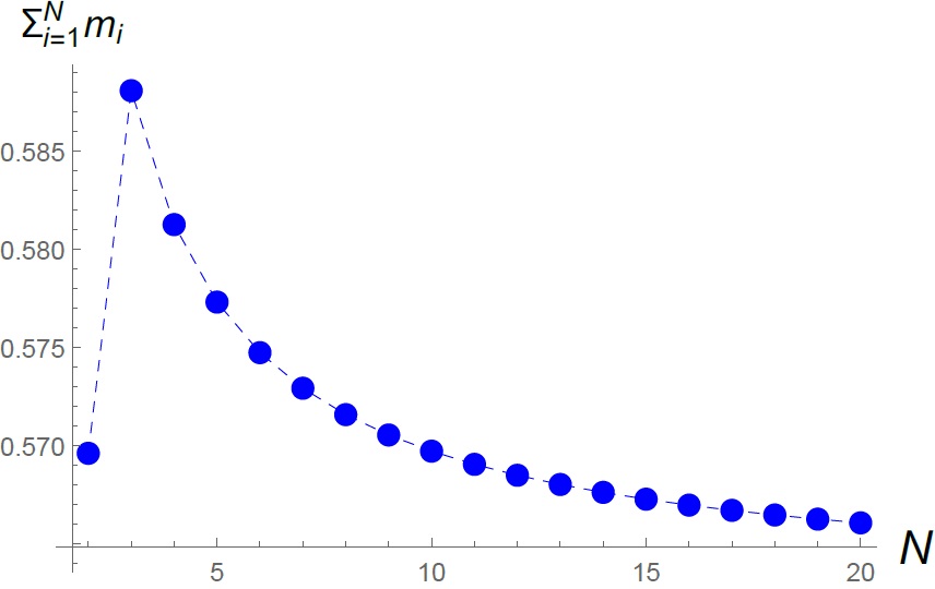
Figure 2: Total Consumer Compensation $(\sigma_{w}=1,\sigma_{e}=0)$

4.3 Unique Implementation

Our analysis thus far has characterized the intermediary’s most preferred equilibrium. An ensuing question is whether the qualitative insights and the asymptotic properties discussed above would hold across all equilibria, particularly in the intermediary’s least preferred equilibrium. A seminal result in the literature on contracting with externalities (see sega99) is the “divide-and-conquer” scheme that guarantees a unique equilibrium outcome (see sewh00 and mish16). Under this scheme, the intermediary can sequentially approach consumers and offer compensation conditional on all earlier consumers having accepted an offer. In this scheme, the first consumer receives compensation equal to her entire surplus loss, thereby guaranteeing her acceptance regardless of the other consumers’ decisions. More generally, consumer $i$ receives the optimal compensation level in the baseline equilibrium when $N=i$.

The cost of acquiring the consumers’ data is strictly higher under “divide and conquer” than in the intermediary’s most preferred equilibrium. Nonetheless, the impact of the ensuring unique implementation on per capita profits vanishes in the limit.

Proposition 7 (“Divide and Conquer”)

Consider the additive data structure with independent errors. Under the “Divide and Conquer” scheme, total consumer compensation satisfies

$$Nm_{i}^{\ast}\leq\frac{3}{4}(1+\log N)(\mathop{\rm var}[\theta_{i}]+\mathop{\rm var}[\varepsilon_{i}]).$$

Under divide and conquer, the total payments to the consumers do not converge to a finite constant as $N$ grows without bound. However, the growth rate of these payments is far smaller than the rate at which the producer’s willingness to pay for data diverges. Therefore, regardless of the equilibrium-selection criterion, the intermediary’s per capita profits converge to the benchmark level when anonymized consumer data are made available.

5 Implications for Consumer Privacy

In this section, we enrich our model along several dimensions to characterize the implications of the optimal data intermediation policy for consumer privacy. In particular, we consider richer pricing instruments in the product market, heterogeneous consumers, heterogeneous product varieties, noisy information collection, and commitment power in the data market.

5.1 Data Anonymization and Social Efficiency

In our baseline setting, data anonymization is optimal independent of the model parameters, such as the number of consumers or the distribution of fundamentals and error terms. This result relies on two crucial assumptions: (i) consumer are homogeneous, by which we mean that the distributions of fundamentals $w$ and errors $e$ are symmetric, and (ii) data sharing has unambiguous welfare effects on product market participants. Indeed, in the model of linear price discrimination, transmitting $X_{i}$ anonymously improves consumer and social surplus, relative to complete data intermediation.

We can generalize this insight to any arbitrary product market interaction beyond the linear pricing model of the previous section. Proposition 8 generalizes the intuition behind the optimal anonymization result in Proposition 3: it establishes that social surplus is the criterion guiding the intermediary’s decision to optimally collect anonymized data.

Proposition 8 (Social Optimality of Data Anonymization)

With homogeneous consumers, anonymized data intermediation is more profitable than complete data intermediation if and only if anonymization increases social surplus.

We note two important aspects of this result. First, it establishes the congruence between the intermediary private objective and the social welfare with respect to the anonymization decision only. It does not claim that the equilibrium information flow itself is socially efficient. Second, the argument does not require any specific feature of the product market interaction. As the decision between anonymization and de-anonymization pertains precisely to the marginal value of the private information of $i$ for the prediction of the willingness to pay $w_{i}$, intermediary and consumer $i$ can attain a socially efficient arrangement.

The result has immediate implications for how equilibrium data sharing policies depend on the nature of the product market interaction. In particular, Proposition 8 allows us to examine the role of richer pricing instruments. bebm15 have shown that every feasible combination of consumer and producer surplus is consistent with some form of price discrimination. Proposition 8 shows that, if the producer had the ability to extract all the expected surplus (given the consumers’ information), then the intermediary would find it more profitable to collect complete, identifying data.

A canonical example where this prediction is relevant is the case of unit demand by the consumers, where our model would predict the prevalence of perfect price discrimination. However, to the extent to which consumers have options to retain some surplus ex post, such as by scaling down their purchase level as in our baseline model, then full surplus extraction would require the producer to have access to more complex pricing mechanisms.

5.2 Market Segmentation and Data

The assumption of ex ante homogeneity among consumers has enabled us to produce some of the central implications of social data. A more complete description of consumer demand should introduce heterogeneity across groups of consumers along characteristics such as location, demographics, income, and wealth.

We now explore how these additional characteristics influence information policy and the profits of the data intermediary. To this end, we augment the description of consumer demand by splitting the population into $J$ homogeneous groups:

$$w_{ij}\sim F_{w,j},~{}e_{i,j}\sim F_{e,j},~{}i=1,2,...,N_{j},~{}j=1,...,J\text{.}$$

The intermediary’s data inflow policy must now specify whether to anonymize the consumers’ signals across groups and within each group. However, Proposition 8 establishes that it is always more profitable to anonymize all signals within each group, rather than revealing the consumers’ identities.

Corollary 4 (No Discrimination within Groups)

The data policy that anonymizes all signals within each group $j=1,...,J$ and only reveals the group identity of each consumer $i$ is more profitable than the complete data-sharing policy.

By further specifying the model, we can identify conditions under which the data intermediary will collect and transmit group characteristics. By collecting information about the group characteristics, the intermediary influences the extent of price discrimination. For example, the intermediary could anonymize all signals across groups, thus forcing the producer to offer only a single price. Alternatively, the intermediary could allow the producer to discriminate between two groups of consumers by recording and transmitting the group identities. As intuition would suggest, enabling price discrimination across groups not only allows the intermediary to charge a higher fee to the producer but also increases the compensation owed to consumers.

Proposition 9 below sheds light on the optimal resolution of this trade-off. In this result, we restrict attention to the case of symmetric groups ($N_{j}=N$ for all $j$), with the additive data structure $w_{i}=\theta+\theta_{i}$, and independent noise terms in the consumers’ signals.

Proposition 9 (Segmentation)

If $N$ is large enough, inducing group-level pricing is more profitable for the intermediary than inducing uniform pricing.

Whereas Proposition 3 stated that the intermediary will not reveal any information about consumer identity, Proposition 9 refines that result: if the market is sufficiently large, then the intermediary will convey limited identity information, i.e., each consumer’s group identity. This policy allows the producer to price discriminate across, but not within, groups. Conversely, if the producer faces few consumers and their willingness to pay are not highly correlated, then pooling all signals reduces the cost of sourcing the data.

The limited amount of price discrimination, which operates optimally at the group level rather than the individual level, can explain the behavior of many platforms. For example, Uber and Amazon claim that they do not discriminate at the individual level, but they condition prices on location, time, and other dimensions that capture group characteristics.

The result in Proposition 9 is perhaps the sharpest manifestation of the value of big data. By enabling the producer to adopt a richer pricing model, a larger database allows the intermediary to extract more surplus. Our result also clarifies the appetite of the platforms for large datasets: because having more consumers allows the platform to profitably segment the market more precisely, the value of the marginal consumer $i=N$ to the intermediary remains large even as $N$ grows. In other words, allowing the producer to segment the market is akin to paying a fixed cost (i.e., higher compensation to the current consumers) to access a better technology (i.e., one that scales more easily with $N$). Figure 3 illustrates this result for an example with normally distributed fundamentals and errors.

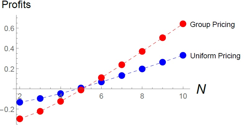
Figure 3: Marginal Value of an Additional Consumer

The optimality of using a richer pricing model when larger datasets are available is reminiscent of model selection criteria under overfitting concerns, e.g., the Akaike information criterion. In our setting, however, the optimality of inducing segmentation is not driven by econometric considerations. Instead, it is entirely driven by the intermediary’s cost-benefit analysis in acquiring more precise information from consumers. As the data externality grows sufficiently strong, acquiring the data becomes cheaper as the intermediary exploits the richer structure of consumer demand.

Finally, the welfare ranking of the two pricing schemes (group vs. uniform) is a priori ambiguous. In particular, group pricing can yield lower total surplus than uniform pricing, e.g., when consumers know their willingness to pay and group pricing results in inefficient price discrimination. In other words, outside of the conditions of Proposition 8 (e.g., with heterogeneous consumers), market segmentation can be driven purely by the data externality.

5.3 Recommender System

In our baseline model, the data shared by the intermediary are used by the producer to set prices and by consumers to learn about their own preferences. The first assumption is, in a sense, the worst-case scenario for the intermediary: consider the case in which consumers’ initial signals are very precise. As price discrimination reduces total surplus, no intermediation would be profitable without a strong, negative data externality. Consequently, data aggregation is an essential part of the optimal data intermediation policy in this case. In practice, however, consumer data can also be used by the producer in surplus-enhancing ways, for example, to facilitate targeting quality levels and other product characteristics to the consumer’s tastes.

In this section, we develop a generalization of our framework; this generalization allows the producer to charge a unit price $p_{i}$ and to offer a product of characteristic $k_{i}$ to each consumer. Consumers differ both in their vertical willingness to pay and in their horizontal taste for the product’s characteristics. Consumer $i$’s utility function is given by

$$u_{i}\left(w_{i},q_{i},p_{i},k_{i},\ell_{i}\right)=(w_{i}-\left(k_{i}-\ell_{i}\right)^{2}-p_{i})q_{i}-q_{i}^{2}/2,$$

with $w_{i}$ denoting the consumer’s willingness to pay and $\ell_{i}$ denoting the consumer’s ideal location or product characteristic. Both the willingness to pay $w\in\mathbb{R}^{N}$ and the locations $\ell\in\mathbb{R}^{N}$ of different consumers are potentially correlated. The producer has a constant marginal cost of quantity provision that we normalize to zero and can freely set the product’s characteristic. Therefore, the case of a common location $\ell_{i}\equiv\ell$ for all consumers yields the baseline model of price discrimination.

We examine the data intermediary’s optimal data inflow policy, which allows for separate aggregation policies for willingness to pay and location information. We impose the following assumptions: (i) the gains from trade under no information sharing are sufficiently large; (ii) the consumers’ fundamentals have a joint Gaussian distribution; and (iii) consumer $i$ perfectly observes $\left(w_{i},\ell_{i}\right)$. The extension to noisy Gaussian signals is immediate. We then obtain another application of Proposition 8.

Proposition 10 (Optimal Aggregation by a Recommender System)

The intermediary’s optimal policy collects anonymized data on the vertical component $w_{i}$ and complete data on the horizontal component $\ell_{i}$.

Therefore, the recommender system enables the producer to offer targeted product characteristics that match $k_{i}$ to $\ell_{i}$ as closely as possible. However, the system does not allow for personalized pricing. The logic is once again given by the intermediary’s sources of profits, i.e., the contribution to social welfare $\Delta W$ and the data externality $DE$. Because the data externalities do not depend on the level of data anonymization, the intermediary chooses to aggregate the vertical dimension of consumer data, thereby reducing the total surplus if transmitted to the producer. Conversely, because the distance between a consumer’s ideal product and the firm’s offer $\left(k_{i}-\ell_{i}\right)^{2}$ shifts the consumer’s demand function down, the intermediary allows for the personalization of product characteristics.

5.4 Intermediary with Commitment

We have assumed thus far that the intermediary cannot refrain from selling information to the producer and cannot sell any acquired data inflow back to the consumers. The latter assumption entails no loss: consumers know that the intermediary sells the data to the producer, and therefore expect to receive all available information regardless of their participation decisions (Proposition 1), because they know that revealing this information maximizes the producer’s fee.

The no commitment assumption reflects the substantial control that large online platforms have over the use of the data and the opacity with which the data outflow is linked to the data inflow. In other words, it is difficult to ascertain how any given data input informs an intermediary’s data output. Nonetheless, it is useful to consider the implications of the data intermediary’s ability to commit to a certain data policy, especially in light of the welfare properties of data sharing discussed above. To that end, suppose the data intermediary offered the consumers contracts that specify a data inflow and a data outflow policy.

Through richer contracts, the data intermediary can offer consumers privacy guarantees. In particular, the intermediary can implement the socially efficient data-sharing policy, which consists of sharing all signals among all the consumers who accept the contract and not sharing any data at all with the producer (Corollary 1). In exchange for this commitment, the data intermediary requests compensation from the consumers. In turn, consumers are willing to pay a positive price for these data, and hence the socially optimal data sharing is always profitable.

However, the equilibrium outcome under these stronger commitment assumptions fails to capture the role of large online platforms. Even though there are examples in which consumers pay a positive price to access tailored, non-sponsored recommendations, data intermediaries choose to monetize the producers’ side of their platform much more frequently. Moreover, the socially efficient policy need not maximize the intermediary’s profits. For example, if fundamentals are perfectly correlated and signals are arbitrarily precise, the intermediary’s profits from the first-best policy are nil. Under these conditions, an intermediary with commitment (or even an intermediary who sells its own products) would not monetize their information by selling it to consumers.

It is beyond the scope of this article to characterize the optimal commitment policy for any initial data structure, but the data externality clearly remains a key driver of the equilibrium allocation of information even under stronger commitment assumptions.

6 Conclusion

We have explored the trading of information between data intermediaries with market power and multiple consumers with correlated preferences. The data externality that we have uncovered strongly suggests that levels of compensation close to zero can induce an individual consumer in a large market to relinquish precise information about her preferences. This finding holds even if the consumer’s data are later sold to a firm that seeks to extract their surplus. Thus, giving consumers control rights over their data (a pillar of privacy regulation such as the EU General Data Protection Regulation or the California Privacy Rights Act) is insufficient to bring about the efficient use of information.

Our results regarding the aggregation of consumer information further suggest that privacy regulations must move away from concerns over personalized prices at the individual level. Most often, firms do not set prices in response to individual-level characteristics. Instead, segmentation of consumers occurs at the group level (e.g., as in the case of Uber) or at the temporal and spatial levels (e.g., as in the case of Staples and Amazon). Thus, our analysis points to the significant welfare effects of group-level and market-level, dynamic prices that react in real time to changes in demand.

A possible mitigator of the consequences of data externalities—echoed in powe18—consists of facilitating the formation of consumer groups or unions to internalize the data externality when bargaining with powerful intermediaries, such as large online platforms. A different regulatory solution is based on privacy managers, such as internet browsers with heterogeneous privacy settings that compete for consumers’ default choice. Yet another solution—suggested by romer19—consists of making the data outflow costly for the intermediary by, for example, taxing targeted advertising. In our model, taxing the data outflow will limit efficient and inefficient intermediation alike but will affect the intermediary’s choice of data policy under the assumptions of Section 5.4.

Finally, our data intermediary collected and redistributed the consumer data but played no role in the interaction between the consumers and the producer. In contrast, a consumer can often access a given producer only through a data platform. Many platforms can then be thought of as auctioning access to the consumer. The data platform provides the bidding producers with additional information that they can use to tailor their interactions with consumers. Social data platforms thus trade individual consumer information for services rather than money. In these markets, the data externality manifests itself in the quality of the services offered and in the extent of the consumers’ engagement.

7 Appendix A

Proof of Lemma 1. Under an arbitrary data-inflow policy $X$, each consumer $i$ observes a noisy signal $S_{i}$ of her own willingness to pay and sends a potentially noisier signal $X_{i}$ to the intermediary. Consumer $i$ observes both $S_{i}$ and $X_{i}$. Given the data inflow $X$, the intermediary chooses an outflow policy, namely, the signal $Y_{0}=Y_{0}(X)$ sent to the producer and the signal $Y_{i}=Y_{i}(X)$ sent to each consumer $i$. The intermediary then chooses a policy $Y$ that maximizes the producer’s ex ante expected payoff, which it fully extracts through the fee $m_{0}$. We let the intermediary selects their favorite equilibrium in the ensuing game.

For any outflow policy $Y=(Y_{0},Y_{i})$, denote an induced signaling equilibrium as $\bar{\gamma}=(\bar{q}_{i},\bar{p})$, where $\bar{p}:Y_{0}\rightarrow R^{+}$ is the pricing strategy of the producer and $\bar{q}_{i}:Y_{i}\times S_{i}\times X_{i}\times R^{+}\rightarrow R^{+}$ is the demand function of consumer $i$. We first argue that there exists an equilibrium $\gamma^{\ast}$ under the outflow policy $(\bar{p}\circ Y_{0},(Y_{i},\bar{p}\circ Y_{0}))$ that yields a weakly higher ex ante payoff for the producer. In this new outflow policy, instead of revealing $Y_{0}$ to the producer, the intermediary directly recommends the price $\bar{p}(Y)$ which coincides with the equilibrium pricing strategy in $\bar{\gamma}$, and reveals to consumer $i$ both $Y_{i}$ and the price recommendation.

On the equilibrium path of $\bar{\gamma}$, consumer $i$ updates her posterior $\mu(Y_{i},S_{i},\bar{p}_{i}(Y))$ using $Y_{i}$, her own private signal $S_{i}$, the report $X_{i}$, and the observed price $p_{i}$. We denote the consumer’s demand as a function of her posterior beliefs and the price as

$$q_{i}(\mu(Y_{i},S_{i},X_{i},p_{i}),p_{i}).$$

The ex ante profit of the producer from consumer $i$ is given by

$$\mathbb{E}\left[\bar{p}_{i}q_{i}(\mu(Y_{i},S_{i},X_{i},\bar{p}_{i}),\bar{p}_{i})\right].$$

Now consider the new outflow policy $(\bar{p}\circ Y_{0},(Y_{i},\bar{p}\circ Y_{0}))$. Under this policy, there exists an equilibrium where consumer $i$ forms her demand using the data outflow $(Y_{i},p^{\ast}\circ Y_{0})$ from the intermediary as well as her own signal $S_{i}$ and the data inflow $X_{i}$. Because consumer $i$ knows everything that the producer knows, the price charged by the producer no longer influences the consumer’s posterior, which therefore coincides with the on-path beliefs in the original equilibrium $\bar{\gamma}$, i.e.,

$$\mu(Y_{i},S_{i},X_{i},\bar{p}_{i}(Y_{0})).$$

Knowing this, the producer maximizes his ex ante payoff by choosing a pricing strategy $\hat{p}(\cdot)$ as a function of his signal $\bar{p}\circ Y_{0}$. Thus the producer’s equilibrium profit is given by

$$\max_{\hat{p}}\hat{p}\big{(}\bar{p}\circ Y_{0}\big{)}q_{i}\Big{(}\mu(Y_{i},S_{i},X_{i},\bar{p}_{i}(Y_{0})),\hat{p}\big{(}\bar{p}\circ Y_{0}\big{)}\Big{)}.$$

Clearly “following the intermediary’s recommendation,” i.e., setting $\hat{p}(p)=p$ is a feasible strategy that yields the same payoff as in the old equilibrium $\bar{\gamma}$. Consequently, the producer’s equilibrium payoff is weakly higher than in $\bar{\gamma}$.   

Proof of Proposition 1. For any offered price $p_{i}$, consumer $i$ demands the quantity

$$q_{i}=\mathbb{E}[w_{i}|(S_{i},Y_{i})]-p_{i}.$$

The producer finds it optimal to set the following price

$$p_{i}=\frac{\mathbb{E}[w_{i}|Y_{0}]}{2}.$$

Recall that the consumer always has superior information so that $Y_{0}$ is measurable with respect to $Y_{i}$. The profit of the producer is given by

$$\Pi_{i}((S_{i},Y_{i}),Y_{0}) =\mathbb{E}\left[\frac{\mathbb{E}[w_{i}|Y_{0}]}{2}\left(\mathbb{E}[w_{i}|(S_{i},Y_{i})]-\frac{\mathbb{E}[w_{i}|Y_{0}]}{2}\right)\right]$$

$$=\frac{\mathbb{E}\left[(\mathbb{E}[w_{i}|Y_{0}])^{2}\right]}{4}=\frac{\mathop{\rm var}[\mathbb{E}[w_{i}|Y_{0}]]+\mathbb{E}[w_{i}]^{2}}{4}$$ (19)

$$=\frac{1}{4}G\left(Y_{0}\right)+\Pi_{i}\left(S_{i},\varnothing\right),$$

where the outside expectation represents integration over the whole probability space. The expected consumer surplus is given by

$$U_{i}((S_{i},Y_{i}),Y_{0}) = \mathbb{E}\left[\left(w_{i}-\frac{\mathbb{E}[w_{i}|Y_{0}]}{2}\right)\left(\mathbb{E}[w_{i}|(S_{i},Y_{i})]-\frac{\mathbb{E}[w_{i}|Y_{0}]}{2}\right)\right]$$

$$-\frac{1}{2}\mathbb{E}\left[\left(\mathbb{E}[w_{i}|(S_{i},Y_{i})]-\frac{\mathbb{E}[w_{i}|Y_{0}]}{2}\right)^{2}\right]$$

$$= \frac{1}{2}\mathbb{E}[(\mathbb{E}[w_{i}|(S_{i},Y_{i})])^{2}-\frac{3}{4}(\mathbb{E}[w_{i}|Y_{0}])^{2}],$$

$$= \frac{1}{2}\left(G\left((S_{i},Y_{i})\right)-G\left(S_{i}\right)\right)-\frac{3}{8}G\left(Y_{0}\right)+U_{i}\left(S_{i},\varnothing\right)$$ (21)

Finally, the impact on total surplus is given by the sum of the two effects:

$$W_{i}\left((S_{i},Y_{i}),Y_{0}\right)-W_{i}\left(S_{i},\varnothing\right)=\frac{1}{2}\left(G\left((S_{i},Y_{i})\right)-G\left(S_{i}\right)\right)-\frac{1}{8}G\left(Y_{0}\right),$$

which completes the proof.   

Proof of Proposition 2. By Lemma 1, it is without loss of generality to assume the producer receives a signal $Y,$ and the consumer receives a signal $(Y_{i},Y)$. Thus, we can focus on equilibria where prices have no signaling effect. These equilibria coincide with those described in Proposition 1. As we have shown there, the profit of the producer is:

$$\mathbb{E}\left[\frac{\mathbb{E}[w_{i}|Y]}{2}\left(\mathbb{E}[w_{i}|Y\cup Y_{i},S_{i},X_{i}]-\frac{\mathbb{E}[w_{i}|Y]}{2}\right)\right]=\frac{\mathbb{E}\left[(\mathbb{E}[w_{i}|Y])^{2}\right]}{4}=\frac{\mathop{\rm var}[\mathbb{E}[w_{i}|Y]]+\mathbb{E}[w_{i}]^{2}}{4}.$$

Therefore it is optimal to maximize $\mathop{\rm var}[\mathbb{E}[w_{i}|Y]]$, which is achieved by setting $Y=X$. Hence,  the intermediary reveals all information collected $\left(Y=X\right)$ both to the producer and to consumer $i$.

 

Proof of Corollary 2. When fundamentals $w_{i}$ are perfectly correlated,

$$\mathbb{E}[w_{i}|S] =\mathbb{E}[\theta|S]=\mathbb{E}[\theta|S_{1},...,S_{N}],$$

$$\mathbb{E}[w_{i}|S_{-i}] =\mathbb{E}[\theta|S_{-i}],$$

$$\mathop{\rm var}[\mathbb{E}[\theta|S_{-i}]] =\mathop{\rm var}[\mathbb{E}[\theta|S_{1},...,S_{N-1}]].$$

Under our symmetry assumption, the variance of the posterior expectation of the common willingness to pay $\mathop{\rm var}[\mathbb{E}[\theta|S_{1,..,N}]]$ can be written as a function of $N$. Now we argue that $\mathop{\rm var}[\mathbb{E}[\theta|S_{1,..,N}]]$ is increasing in $N$. We first define $g(S_{1,...,N-1})\triangleq\mathbb{E}[\theta|S_{1,..,N-1}]$. Then, according to Lemma 3 below, we have

$$\mathop{\rm var}[\mathbb{E}[\theta|S_{1,..,N}]] =\max_{f\in L^{2}}~{}\mathop{\rm var}[\theta]-\mathbb{E}[(\theta-g(S_{1,...,N}))^{2}],$$

$$\geq\max_{f\in L^{2}}~{}\mathop{\rm var}[\theta]-\mathbb{E}[(\theta-g(S_{1,...,N-1}))^{2}],$$

$$=\mathop{\rm var}[\mathbb{E}[\theta|S_{1,..,N-1}]].$$

The sequence $\mathop{\rm var}[\mathbb{E}[\theta|S_{1,..,N}]]$ is increasing and bounded. Therefore, it converges:

$$\lim_{N\rightarrow\infty}G(S)=\lim_{N\rightarrow\infty}G(S_{-i}),$$

and intermediation is then profitable:

$$\lim_{N\rightarrow\infty}\frac{R(S)}{N}=\frac{1}{4}\lim_{N\rightarrow\infty}G(S)>0.$$

In the limit for $N\rightarrow\infty$, the data externality and the consumer surplus are given by

$$\lim_{N\rightarrow\infty}U_{i}(S,S)-U_{i}(S_{i},\varnothing) =\lim_{N\rightarrow\infty}\mathbb{E}[\frac{1}{8}(\mathbb{E}[w_{i}|S])^{2}-\frac{1}{2}(\mathbb{E}[w_{i}|S_{i}]-\mathbb{E}[w_{i}])^{2}-\frac{1}{8}\mathbb{E}[w_{i}]^{2}]$$

$$=\lim_{N\rightarrow\infty}\frac{1}{8}\mathop{\rm var}[\mathbb{E}[w_{i}|S]]-\frac{1}{2}\mathop{\rm var}[\mathbb{E}[w_{i}|S_{i}]],$$

$$\lim_{N\rightarrow\infty}DE_{i}(S) =\lim_{N\rightarrow\infty}\frac{1}{2}\mathop{\rm var}[\mathbb{E}[w_{i}|S]]-\frac{1}{2}\mathop{\rm var}[\mathbb{E}[w_{i}|S_{i}]]-\frac{3}{8}\mathop{\rm var}[\mathbb{E}[w_{i}|S_{-i}]]$$

$$=\lim_{N\rightarrow\infty}\frac{1}{8}\mathop{\rm var}[\mathbb{E}[w_{i}|S]]-\frac{1}{2}\mathop{\rm var}[\mathbb{E}[w_{i}|S_{i}]].$$

Therefore, when the initial noise is sufficiently small (i.e., when $\mathop{\rm var}[\mathbb{E}[w_{i}|S_{i}]]$ is close to $\mathop{\rm var}[w_{i}]$), the data externality is negative and data sharing hurts consumers.   

Proof of Corollary 3. Because $w_{i}$ is independent from the other consumers’ signals, we have $\mathop{\rm var}[\mathbb{E}[w_{i}|S_{-i}]]=0$. Thus, intermediation is always unprofitable, and the data externality is always positive,

$$R(S) =-\frac{N}{8}\mathop{\rm var}[\mathbb{E}[w_{i}|S]]<0,$$

$$DE_{i}(S) =\frac{1}{2}(\mathop{\rm var}[\mathbb{E}[w_{i}|S]]-\mathop{\rm var}[\mathbb{E}[w_{i}|S_{i}]])\geq 0.$$

Finally, for the results on consumer surplus, we turn to Lemma 3. In particular, we know

$$\mathop{\rm var}[\mathbb{E}[w_{i}|S]] =\mathop{\rm var}[w_{i}]-\mathbb{E}[(w_{i}-\mathbb{E}[w_{i}|S])^{2}],$$

$$\geq\mathop{\rm var}[w_{i}]-\mathbb{E}[(w_{i}-(s_{i}-\frac{1}{N-1}\Sigma_{j\neq i}s_{j}))^{2}],$$

$$=\mathop{\rm var}[\theta_{i}]-\mathbb{E}[(\theta_{i}-(\theta_{i}+\varepsilon-\frac{1}{N-1}\Sigma_{j\neq i}\theta_{j}-\varepsilon))^{2}],$$

$$=\mathop{\rm var}[\theta_{i}]-\mathbb{E}[(\frac{1}{N-1}\Sigma_{j\neq i}\theta_{j})^{2}]=\frac{N-2}{N-1}\mathop{\rm var}[\theta_{i}]\rightarrow\mathop{\rm var}[w_{i}].$$

Thus we obtain

$$\lim_{N\rightarrow\infty}U_{i}(S,S)-U_{i}(S_{i},\varnothing)=\frac{1}{8}\mathop{\rm var}[w_{i}]-\frac{1}{2}\mathop{\rm var}[\mathbb{E}[w_{i}|S_{i}]].$$

When $\sigma$ is sufficiently large, so that $\mathop{\rm var}[\mathbb{E}[w_{i}|S_{i}]]$ is close to $0$, intermediation increases consumer surplus.   

The proof of Proposition 2 follows from expressions (15) and (16) in the text.

Proof of Proposition 3. In the main text, the data inflow from consumer $i$ is given by $X_{i}=S_{i}$ (under complete sharing) and we compare it with $X_{i}^{\ast}=\delta\left(S_{i}\right)$ (under anonymization). Note that $(S_{i},X_{i})_{i}$ in this case is symmetrically distributed, i.e., its joint density is unchanged under permutations of indices. Here we prove a slightly more general version of the result by allowing an arbitrary information inflow $X$ such that $(S_{i},X_{i})_{i}$ is symmetrically distributed. We assume that apart from the private signal $S_{i}$ and information outflow $Y_{i}$ provided by the intermediary, consumer $i$ also observes her own data inflow $X_{i}$. This assumption is needed because information set $(S_{i},X_{i},X_{-i}^{\ast})$ and $(S_{i},X_{i},X^{\ast})$ are equivalent by construction, but $(S_{i},X_{-i}^{\ast})$ and $(S_{i},X^{\ast})$ maybe not. Note that when we restrict to the less general case (when $X_{i}=S_{i}$), the latter holds automatically, so we do not need this assumption.

For any fixed inflow policy $X$, we refer to $p_{-i}$ as the off-path price charged to consumer $i$ when she does not accept the intermediary’s contract, and to $p_{i}$ as the on-path price charged to consumer $i$. Now consider another inflow policy $X^{\ast}$ identical to $X$ up to a random permutation of the consumers’ identities. Under this scheme, we refer to $p_{-i}^{\ast}$ as the off-path price for consumer $i$, and to $p_{i}^{\ast}$ as the on-path price for consumer $i$.

We first argue that $p_{-i}=p_{-i}^{\ast}$ for any realization of $W,S,X$. To do so, let us calculate consumer $i$’s posterior about $W_{i}$ under each inflow policy. Under the non-anonymized scheme, the posterior distribution of consumer $i$’s willingness to pay is given by

$$f_{i}(W_{i} =w_{i}|S_{i}=s_{i},X_{i}=x_{i},X=x)$$

$$=\frac{\int f(W_{i}=w_{i},W_{-i}=w_{-i}^{\prime},S_{i}=s_{i},S_{-i}=s_{-i}^{\prime},X_{i}=x_{i},X_{-i}=x_{-i})\text{d}s_{-i}^{\prime}\text{d}w_{-i}^{\prime}}{\int f(W=w^{\prime},S_{i}=s_{i},S_{-i}=s_{-i}^{\prime},X_{i}=x_{i},X_{-i}=x_{-i})\text{d}s_{-i}^{\prime}\text{d}w^{\prime}}.$$

Recall from Proposition 2 that the intermediary’s optimal data outflow policy consists of revealing to the consumers all the available information, even if the consumer refuses to participate. When the data is anonymized, because consumer $i$ knows her own report $X_{i}$, the data outflow reveals to her the vector of reports $X_{-i}$ without knowing who generated each one. We now define $\delta\in S^{n-1}$ as permutation of consumer indices. Consumer $i$’s posterior distribution over her willingness to pay $w_{i}$ is now given by

$$f_{i}(W_{i}=w_{i}|S_{i}=s_{i},X_{i}=x_{i},X_{-i}^{\ast}=x_{-i}).$$

For notational simplicity, we use $Pr$ to denote both probability and the proper marginal density. Then the posterior can be rewritten as

$$\frac{\Pr(W_{i}=w_{i},S_{i}=s_{i},X_{i}=x_{i},X_{-i}^{\ast}=x_{-i})}{\Pr(S_{i}=s_{i},X_{i}=x_{i},X_{-i}^{\ast}=x_{-i})}$$

$$=\frac{\Sigma_{\delta\in S^{n-1}}\Pr(\delta,W_{i}=w_{i},S_{i}=s_{i},X_{i}=x_{i},X_{-i}=x_{\delta(-i)})}{\Sigma_{\delta\in S^{n-1}}\Pr(\delta,S_{i}=s_{i},X_{i}=x_{i},X_{-i}=x_{\delta(-i)})}$$

$$=\frac{\Sigma_{\delta\in S^{n-1}}\Pr(\delta)\Pr(W_{i}=w_{i},S_{i}=s_{i},X_{i}=x_{i},X_{-i}=x_{\delta(-i)})}{\Sigma_{\delta\in S^{n-1}}\Pr(\delta)Pr(S_{i}=s_{i},X_{i}=x_{i},X_{-i}=x_{\delta(-i)})}.$$

Because of the symmetry assumption, we know that

$$\Pr(W_{i}=w_{i},S_{i}=s_{i},X_{i}=x_{i},X_{-i}=x_{\delta(-i)})$$

$$=\int f(W_{i}=w_{i},W_{-i}=w_{-i}^{\prime},S_{i}=s_{i},S_{-i}=s_{-i}^{\prime},X_{i}=x_{i},X_{-i}=x_{\delta(-i)})\text{d}s_{-i}^{\prime}\text{d}w_{-i}^{\prime}$$

$$=\int f(W_{i}=w_{i},W_{-i}=w_{\delta^{-1}(-i)}^{\prime},S_{i}=s_{i},S_{-i}=s_{\delta^{-1}(-i)}^{\prime},X_{i}=x_{i},X_{-i}=x_{-i})\text{d}s_{-i}^{\prime}\text{d}w_{-i}^{\prime}$$

$$=\int f(W_{i}=w_{i},W_{-i}=w_{\delta^{-1}(-i)}^{\prime},S_{i}=s_{i},S_{-i}=s_{\delta^{-1}(-i)}^{\prime},X_{i}=x_{i},X_{-i}=x_{-i})\text{d}s_{\delta^{-1}(-i)}^{\prime}\text{d}w_{\delta^{-1}(-i)}^{\prime}$$

$$=\Pr(W_{i}=w_{i},S_{i}=s_{i},X_{i}=x_{i},X_{-i}=x_{-i}).$$

For the same reason, we also have

$$\Pr(S_{i}=s_{i},X_{i}=x_{i},X_{-i}=x_{\delta(-i)})=\Pr(S_{i}=s_{i},X_{i}=x_{i},X_{-i}=x_{-i}).$$

Thus the posterior of consumer $i$ can be simplified as:

$$f_{i}(W_{i} =w_{i}|S_{i}=s_{i},X_{i}=x_{i},X_{-i}^{\ast}=x_{-i})$$

$$=\frac{\Sigma_{\delta\in S^{n-1}}\Pr(\delta)\Pr(W_{i}=w_{i},S_{i}=s_{i},X_{i}=x_{i},X_{-i}=x_{-i})}{\Sigma_{\delta\in S^{n-1}}\Pr(\delta)Pr(S_{i}=s_{i},X_{i}=x_{i},X_{-i}=x_{-i})}$$

$$=\frac{\Sigma_{\delta\in S^{n-1}}\frac{1}{|S^{n-1}|}\Pr(W_{i}=w_{i},S_{i}=s_{i},X_{i}=x_{i},X_{-i}=x_{-i})}{\Sigma_{\delta\in S^{n-1}}\frac{1}{|S^{n-1}|}\Pr(S_{i}=s_{i},X_{i}=x_{i},X_{-i}=x_{-i})}$$

$$=f_{i}(W_{i}=w_{i}|S_{i}=s_{i},X_{i}=x_{i},X_{-i}=x_{-i}).$$

We have therefore proved that consumer $i$ has the same posterior about her willingness to pay $w_{i}$ for any realization of $W,S,X$ irrespective of whether the data are anonymized of not. Furthermore, this holds both on and off the path of play.

Next, we show that the producer also has the same posterior about $W_{i}$ for any realization of $W,S,X$ when consumer $i$ refuses to report. Under the non-anonymized scheme, the posterior density is given by:

$$f_{i}(W_{i}=w_{i}|X=x)=\frac{\int f(W_{i}=w_{i},W_{-i}=w_{-i}^{\prime},S=s^{\prime},X_{i}=x_{i},X_{-i}=x_{-i})\text{d}s^{\prime}\text{d}w_{-i}^{\prime}}{\int f(W=w^{\prime},S=s^{\prime},X=x_{i},X_{-i}=x_{-i})\text{d}s^{\prime}\text{d}w^{\prime}}.$$

Under the anonymized scheme, the posterior density is given by

$$f_{i}(W_{i}=w_{i}|X^{\ast}=x)=\frac{\Sigma_{\delta\in S^{n-1}}\Pr(\delta)\Pr(W_{i}=w_{i},X=\delta(x))}{\Sigma_{\delta\in S^{n-1}}\Pr(\delta)\Pr(X=\delta(x))}$$

By the earlier argument, we can simplify it as follows:

$$\frac{\Sigma_{\delta\in S^{n-1}}\Pr(\delta)\Pr(W_{i}=w_{i},X=x)}{\Sigma_{\delta\in S^{n-1}}\Pr(\delta)\Pr(X=x)}=f_{i}(W_{i}=w_{i}|X=x)$$

Because the posteriors for both parties are the same for any realization, so is the price, and hence the welfare impact of information

The profit of the intermediary from consumer $i$’s data under inflow policy $X$ is given by

$$R_{i}\left(X\right)=\Pi(X,X)-\Pi(S_{i},\varnothing)-U_{i}((S_{i},X_{-i}),X_{-i})+U_{i}((S_{i},X),X).$$

We have argued that consumer surplus off the path is the same:

$$U_{i}((S_{i},X_{-i}),X_{-i})=U_{i}((S_{i},X^{\ast}_{-i}),X_{-i}^{\ast}).$$

We now turn to the last term—the impact on social welfare on the path of play:

$$\Pi((S_{i},X),X)+U_{i}((S_{i},X),X)$$

$$=\frac{1}{2}\mathbb{E}[(\mathbb{E}[w_{i}|S_{i},X_{i},X]-\mathbb{E}[w_{i}|X])^{2}+\frac{1}{4}(\mathbb{E}[w_{i}|X])^{2}]+\frac{\mathop{\rm var}[\mathbb{E}[w_{i}|X]]}{4}$$

$$=\frac{1}{2}\mathop{\rm var}[\mathbb{E}[w_{i}|S_{i},X_{i},X]]-\frac{1}{8}\mathop{\rm var}[\mathbb{E}[w_{i}|X]].$$

Recall that consumer $i$ has the same on path posterior under two different scheme. Therefore, the difference in the intermediary’s profits under the two policies reduces to

$$\frac{1}{2}\mathop{\rm var}[\mathbb{E}[w_{i}|S_{i},X_{i},X]]-\frac{1}{8}\mathop{\rm var}[\mathbb{E}[w_{i}|X]]-\frac{1}{2}\mathop{\rm var}[\mathbb{E}[w_{i}|S_{i},X_{i},X^{\ast}]]+\frac{1}{8}\mathop{\rm var}[\mathbb{E}[w_{i}|X^{\ast}]]$$

$$=-\frac{1}{8}\mathop{\rm var}[\mathbb{E}[w_{i}|X]]+\frac{1}{8}\mathop{\rm var}[\mathbb{E}[w_{i}|X^{\ast}]]\leq 0.$$

Therefore, anonymization is more profitable than complete sharing, and strictly so whenever anonymization makes the estimation less precise.   

In the remainder of the Appendix, we often make use of the following classical result in statistics, which we state as a lemma without proof—the result is an immediate consequence of the fact that $\mathbb{E}[X|Y]$ is the projection of $X$ on $\mathcal{F}(Y)$ in $L^{2}$ space.

Lemma 3

Let $W$ and $Y$ be two random variables. Then it holds that

$$\mathop{\rm var}[\mathbb{E}[W|Y]]=\mathop{\rm var}[W]-\mathbb{E}[(W-\mathbb{E}[W|Y])^{2}]\leq\mathop{\rm var}[W],$$

and

$$\text{ }\mathbb{E}[(W-\mathbb{E}[W|Y])^{2}]\leq\mathbb{E}[(W-f(Y))^{2}],\quad\forall f\in L^{2}.$$

To prove Proposition 4, we first state a basic property of anonymized data sharing in our symmetric environment.

Lemma 4

When the data is anonymized, the following holds:

$$\mathbb{E}[w_{i}|A]=\mathbb{E}[w_{j}|A].$$

Proof of Lemma 4. Denote the joint distribution of $W$ and $S$ as $f(W=w,S=s)$ and the posterior of $W_{i}$ after observing $A$ as $f(W_{i}=w|A)$. Denote the permutation in $S^{N}$ as $\nu$ and especially the swapping between $i$ and $j$ as $\nu_{ij}$. For notational simplicity, we use $\Pr$ to denote both probability and the proper marginal density.

$$f_{i}(W_{i} =w_{i}|A=s)=\frac{\Pr(W_{i}=w_{i},A=s)}{\Pr(A=s)}=\frac{\Sigma_{\nu\in S^{N}}\Pr(\nu)\Pr(W_{i}=w_{i},S_{\nu}=s))}{\Pr(A=s)}$$

$$=\frac{\Sigma_{\nu\in S^{N}}\frac{1}{|S^{N}|}\int f(W_{i}=w_{i},W_{j}=w_{j},W_{-ij}=w_{-ij},S_{\nu}=s)\text{d}w_{j}\text{d}w_{-ij}}{\Pr(A=s)}.$$

Because $f$ is unchanged under permutation, we can apply the following transformation:

$$f_{i}(W_{i}=w_{i}|A=s)=\frac{\Sigma_{\nu\in S^{N}}\frac{1}{|S^{N}|}\int f(W_{j}=w_{i},W_{i}=w_{j},W_{-ij}=w_{-ij},S_{\nu_{ij}\circ\nu}=s)\text{d}w_{j}\text{d}w_{-ij}}{\Pr(A=s)},$$

$$=\frac{\Sigma_{\nu_{ij}\circ\nu\in S^{N}}\frac{1}{|S^{N}|}\int f(W_{j}=w_{i},W_{i}=w_{i}^{\prime},W_{-ij}=w_{-ij},S_{\nu_{ij}\circ\nu}=s)\text{d}w_{i}^{\prime}\text{d}w_{-ij}}{\Pr(A=s)}=f_{j}(W_{j}=w_{i}|A=s).$$

Because the posterior distribution is the same, so is the conditional expectation because

$$\mathbb{E}[w_{i}|A]=\int w_{i}f_{i}(W_{i}=w_{i}|A)\text{d}w_{i},$$

which completes the proof.

 

Proof of Proposition 4. Combining Lemmas 3 and 4, we obtain

$$\mathbb{E}[w_{i}|A] =\mathbb{E}[\frac{1}{N}\Sigma_{i}w_{i}|A]=\mathbb{E}[\theta+\frac{1}{N}\Sigma_{i}\theta_{i}|A];$$

$$G(A) =\mathop{\rm var}[\mathbb{E}[\theta+\frac{1}{N}\Sigma_{i}\theta_{i}|A]]=\mathop{\rm var}[\theta+\frac{1}{N}\Sigma_{i}\theta_{i}]-\mathbb{E}[(\theta+\frac{1}{N}\Sigma_{i}\theta_{i}-\mathbb{E}[\theta+\frac{1}{N}\Sigma_{i}\theta_{i}|A])^{2}].$$

We can simplify the last term as follows:

$$\mathbb{E}[(\theta+\frac{1}{N}\Sigma_{i}\theta_{i}-\mathbb{E}[\theta+\frac{1}{N}\Sigma_{i}\theta_{i}|A])^{2}]$$

$$=\mathbb{E}[(\theta-\mathbb{E}[\theta|A])^{2}+\frac{1}{N^{2}}(\Sigma_{i}\theta_{i}-\Sigma_{i}\mathbb{E}[\theta_{i}|A])^{2}-\frac{2}{N}(\theta-\mathbb{E}[\theta|A])(\Sigma_{i}\theta_{i}-\Sigma_{i}\mathbb{E}[\theta_{i}|A])]$$

$$\geq\mathbb{E}[(\theta-\mathbb{E}[\theta|A])^{2}]-\frac{2}{N}\sqrt{\mathop{\rm var}[\theta-\mathbb{E}[\theta|A]]\mathop{\rm var}[\Sigma_{i}\theta_{i}-\Sigma_{i}\mathbb{E}[\theta_{i}|A]]}$$

$$\geq\mathbb{E}[(\theta-\mathbb{E}[\theta|A])^{2}]-\frac{2}{N}\sqrt{N\mathop{\rm var}[\theta]\mathop{\rm var}[\theta_{i}]},$$

where the last inequality comes from Lemma 3. The intermediary’s profit can be written as

$$R =3G(A_{-i})-G(A),$$

$$=3\mathop{\rm var}[\mathbb{E}[\theta|A_{-i}]]-\mathop{\rm var}[\theta]-\frac{1}{N}\mathop{\rm var}[\theta_{i}]+\mathbb{E}[(\theta+\frac{1}{N}\Sigma_{i}\theta_{i}-\mathbb{E}[\theta+\frac{1}{N}\Sigma_{i}\theta_{i}|A])^{2}],$$

$$\geq 3\mathop{\rm var}[\mathbb{E}[\theta|A_{-i}]]-\mathop{\rm var}[\theta]-\frac{1}{N}\mathop{\rm var}[\theta_{i}]+\mathbb{E}[(\theta-\mathbb{E}[\theta|A])^{2}]-\frac{2}{N}\sqrt{N\mathop{\rm var}[\theta]\mathop{\rm var}[\theta_{i}]}$$

$$=3\mathop{\rm var}[\mathbb{E}[\theta|A_{-i}]]-\mathop{\rm var}[\mathbb{E}[\theta|A]]-\frac{1}{N}\mathop{\rm var}[\theta_{i}]-\frac{2}{\sqrt{N}}\sqrt{\mathop{\rm var}[\theta]\mathop{\rm var}[\theta_{i}]}.$$

Therefore, in the limit we have:

$$\lim_{N\rightarrow\infty}R=2\lim_{N\rightarrow\infty}\mathop{\rm var}[\mathbb{E}[\theta|A]]>0,$$

which completes the proof.

 

Proof of Proposition 5. We first prove that the total compensation is bounded from above, which immediately implies that the individual compensation goes to $0$ as $N\rightarrow\infty$. From Lemma 4, we know that

$$G(A) =\mathop{\rm var}[\mathbb{E}[w_{i}|A]]=\mathop{\rm var}[\mathbb{E}[\Sigma_{i}\frac{w_{i}}{N}|A]],$$

$$\leq\mathop{\rm var}[\Sigma_{i}\frac{w_{i}}{N}]=\mathop{\rm var}[\theta]+\frac{\mathop{\rm var}[\theta_{i}]+\mathop{\rm var}[\varepsilon_{i}]}{N}.$$

On the other hand, we also know

$$G(A_{-i})=\mathop{\rm var}[\mathbb{E}[\theta|A_{-i}]]=\mathop{\rm var}[\theta]-\mathbb{E}[(\theta-\mathbb{E}[\theta|A_{-i}])^{2}].$$

Because the conditional expectation is the best $L^{2}$ approximation, we know it leads to a smaller error than the “sample average estimator,”

$$\mathbb{E}\left[(\theta-\mathbb{E}[\theta|A_{-i}])^{2}\right]\leq\mathbb{E}\left[\theta-\frac{1}{N-1}\Sigma_{j\neq i}(\theta+\theta_{j}+\varepsilon_{j})^{2}\right]=\frac{1}{N-1}(\mathop{\rm var}[\theta_{i}]+\mathop{\rm var}[\varepsilon_{j}]).$$

Therefore, we have:

$$N(G(A)-G(A_{-i})) \leq N\Big{(}\mathop{\rm var}[\theta]+\frac{\mathop{\rm var}[\theta_{i}]+\mathop{\rm var}[\varepsilon_{i}]}{N}-\mathop{\rm var}[\theta]+\frac{1}{N-1}(\mathop{\rm var}[\theta_{i}]+\mathop{\rm var}[\varepsilon_{j}])\Big{)},$$

$$=N\left(\frac{\mathop{\rm var}[\theta_{i}]+\mathop{\rm var}[\varepsilon_{i}]}{N}+\frac{1}{N-1}(\mathop{\rm var}[\theta_{i}]+\mathop{\rm var}[\varepsilon_{i}])\right)$$

$$\leq 3(\mathop{\rm var}[\theta_{i}]+\mathop{\rm var}[\varepsilon_{i}]).$$

The total consumer compensation is then given by

$$\frac{3N}{8}(G(A)-G(A_{-i}))\leq\frac{9}{8}(\mathop{\rm var}[\theta_{i}]+\mathop{\rm var}[\varepsilon_{i}]).$$

Finally, the intermediary’s profit is growing linearly in $N$ because

$$R(S) =\frac{N}{4}G(A)-\frac{3N}{8}(G(A)-G(A_{-i})),$$

$$\lim_{N\rightarrow\infty}\frac{R(S)}{N} =\frac{1}{4}\lim_{N\rightarrow\infty}G(A),$$

which completes the proof.

 

Proof of Proposition 6. When data is not anonymized we have:

$$G(S)-G(S_{-i})=\mathop{\rm var}[\mathbb{E}[\theta+\theta_{i}|S]]-\mathop{\rm var}[\mathbb{E}[\theta|S_{-i}]].$$

Because of symmetry, we have

$$\mathop{\rm cov}[\mathbb{E}[\theta|S],\mathbb{E}[\theta_{i}|S]]=\mathop{\rm cov}[\mathbb{E}[\theta|S],\mathbb{E}[\theta_{j}|S]]=\mathop{\rm cov}[\mathbb{E}[\theta|S],\Sigma_{j=1}^{N}\mathbb{E}[\theta_{j}/N\left|S\right.]].$$

Because the correlation coefficient is always greater than $-1$, we obtain

$$\mathop{\rm cov}[\mathbb{E}[\theta|S],\Sigma_{j=1}^{N}\mathbb{E}[\theta_{j}/N\left|S\right.]] \geq-\sqrt{\mathop{\rm var}[\theta]\mathop{\rm var}[\Sigma_{j=1}^{N}\mathbb{E}[\theta_{j}/N\left|S\right.]]},$$

$$\geq-\sqrt{\mathop{\rm var}[\theta]\mathop{\rm var}[\Sigma_{j=1}^{N}\theta_{j}/N]}.$$

Therefore, according to Lemma 3 we have:

$$G(S)-G(S_{-i}) =\mathop{\rm var}[\mathbb{E}[\theta|S]]+2\mathop{\rm cov}[\mathbb{E}[\theta|S],\mathbb{E}[\theta_{i}|S]]+\mathop{\rm var}[\mathbb{E}[\theta_{i}|S]]-\mathop{\rm var}[\mathbb{E}[\theta|S_{-i}]]$$

$$\geq\mathop{\rm var}[\mathbb{E}[\theta|S]]-2\frac{1}{\sqrt{N}}\sqrt{\mathop{\rm var}[\theta]\mathop{\rm var}[\theta_{i}]}+\mathop{\rm var}[\mathbb{E}[\theta_{i}|S]]-\mathop{\rm var}[\mathbb{E}[\theta|S_{-i}]],$$

and hence

$$\liminf_{N\rightarrow\infty}G(S)-G(S_{-i})\geq\mathop{\rm var}[\mathbb{E}[\theta_{i}|S]].$$

The last term is strictly positive because

$$\mathop{\rm var}[\mathbb{E}[\theta_{i}|S]] =\mathop{\rm var}[\theta_{i}]-\mathbb{E}[(\theta_{i}-\mathbb{E}[\theta_{i}|S])^{2}]$$

$$\geq\mathop{\rm var}[\theta_{i}]-\mathbb{E}[(\theta_{i}-\frac{\mathop{\rm var}[\theta_{i}]}{\mathop{\rm var}[\theta_{i}]+\mathop{\rm var}[\theta]+\mathop{\rm var}[e]}S_{i})^{2}],$$

$$=\mathop{\rm var}[\theta_{i}]-(\mathop{\rm var}[\theta_{i}]-\frac{\mathop{\rm var}^{2}[\theta_{i}]}{\mathop{\rm var}[\theta_{i}]+\mathop{\rm var}[\theta]+\mathop{\rm var}[e]}),$$

$$=\frac{\mathop{\rm var}^{2}[\theta_{i}]}{\mathop{\rm var}[\theta_{i}]+\mathop{\rm var}[\theta]+\mathop{\rm var}[e]}>0,$$

where the first inequality again uses Lemma 3.   

Proof of Proposition 7. In the standard “divide and conquer” scheme, the compensation for the $i$-th consumer is the marginal loss of revealing her information given that $i-1$ consumers reveal their signals:

$$\frac{3}{8}G(S_{1,...,i})-\frac{3}{8}G(S_{1,...,i-1}).$$

Because in general we do not know whether this marginal loss is decreasing in $i$, we consider the following revised version of divide and conquer, where consumer $i$ receives

$$m_{i}=\max_{k\geq i}\frac{3}{8}G(S_{1,...,k})-\frac{3}{8}G(S_{1,...,k-1}).$$

Under this payment scheme, it is a dominant strategy for consumer $1$ to accept the offer. Moreover, it is optimal for consumer $i$ to accept the offer, given that the first $i-1$ consumers accept. Using an identical proof to Proposition 5, we obtain

$$\frac{3}{8}G(S_{1,...,i})-\frac{3}{8}G(S_{1,...,i-1}) \leq\frac{3}{8}(\frac{1}{i}+\frac{1}{i-1})(\mathop{\rm var}[\theta_{i}]+\mathop{\rm var}[\varepsilon_{i}]),$$

$$\leq\frac{3}{4}\frac{1}{i-1}(\mathop{\rm var}[\theta_{i}]+\mathop{\rm var}[\varepsilon_{i}]).$$

Therefore, we obtain an upper bound on the compensation paid to consumer $i$ :

$$m_{i}\leq\max_{k\geq i}\frac{3}{4}\frac{1}{k-1}(\mathop{\rm var}[\theta_{i}]+\mathop{\rm var}[\varepsilon_{i}])=\frac{3}{4}\frac{1}{i-1}(\mathop{\rm var}[\theta_{i}]+\mathop{\rm var}[\varepsilon_{i}]).$$

Finally, because we have

$$\Sigma_{i}\frac{3}{8}(G(S_{1,...,i})-G(S_{1,...,i-1})) \leq\frac{3}{4}(1+\Sigma_{i=3}^{N}\frac{1}{i-1})(\mathop{\rm var}[\theta_{i}]+\mathop{\rm var}[\varepsilon_{i}]),$$

$$\leq\frac{3}{4}(1+\log N)(\mathop{\rm var}[\theta_{i}]+\mathop{\rm var}[\varepsilon_{i}]),$$

the total compensation grows at a speed less than $\log N$.   

Proof of Proposition 8. The proof of this proposition is similar to that of Proposition 3. By Lemma 1, we know that the intermediary will transmit whatever information it collected to all consumers. By homogeneity, we know the consumer’s posterior about their own fundamental $w_{ij}$ is the same whether the signals are anonymized or not, and the producer’s posterior about any deviating consumer’s fundamental is also the same under the two schemes.

Denote the broker’s revenue under the non-anonymized and anonymized scheme as $R(X)$ and $R(X^{\ast})$, respectively. It then holds that

$$R_{i}\left(X\right) =\Pi(X,X)-\Pi(S_{i},\varnothing)-U_{i}((S_{i},X_{-i}),X_{-i})+U_{i}((S_{i},X),X),$$

$$R_{i}\left(X^{\ast}\right) =\Pi(X^{\ast},X^{\ast})-\Pi(S_{i},\varnothing)-U_{i}((S_{i},X_{-i}^{\ast}),X_{-i}^{\ast})+U_{i}((S_{i},X^{\ast}),X^{\ast}).$$

Our analysis in previous paragraph implies

$$U_{i}((S_{i},X_{-i}),X_{-i})=U_{i}((S_{i},X_{-i}^{\ast}),X_{-i}^{\ast}).$$

Therefore the intermediary prefers anonymization if and only if

$$R_{i}(X^{\ast})-R_{i}(X)=W((S_{i},X^{\ast}),X^{\ast})-W((S_{i},X),X)\geq 0,$$

which completes the proof.   

Proof of Proposition 9. We first consider the case where the intermediary anonymizes all data, including the group identities. Similar to the result in Lemma 4 (A.2 in the latest draft), we know that the producer offers one price to all consumers on the path of play,

$$\mathbb{E}[w_{ij}|A]=\mathbb{E}[w_{i^{\prime}j^{\prime}}|A].$$

Denoting $N=\Sigma_{j}N_{j}$, we have

$$\mathbb{E}[w_{i^{\prime}j^{\prime}}|A] =\frac{1}{\Sigma_{j}N_{j}}\Sigma_{j}\Sigma_{i}\mathbb{E}[w_{ij}|A]=\frac{1}{\Sigma_{j}N_{j}}\Sigma_{j}\Sigma_{i}\mathbb{E}[\theta_{j}+\theta_{ij}|A]$$

$$=\Sigma_{j}\frac{N_{j}}{N}\mathbb{E}[\theta_{j}|A]+\frac{1}{N}\mathbb{E}[\Sigma_{ji}\theta_{ij}|A].$$

Therefore we obtain an upper bound on the revenue per capita

$$\frac{R(A)}{N} =\frac{3}{8}G(A_{-ij})-\frac{1}{8}G(A)=\frac{3}{8}[\mathbb{E}[w_{ij}]|A_{-ij}]-\frac{1}{8}\mathop{\rm var}[\mathbb{E}[w_{ij}]|A]$$

$$\leq\frac{1}{4}\mathop{\rm var}[\mathbb{E}[w_{ij}]|A]=\frac{1}{4}\mathop{\rm var}[\Sigma_{j}\frac{N_{j}}{N}\mathbb{E}[\theta_{j}|A]+\frac{1}{N}\mathbb{E}[\Sigma_{ji}\theta_{ij}|A]]$$

$$\leq\frac{1}{4}\frac{1}{N^{2}}\Sigma N_{j}^{2}\mathop{\rm var}[\theta_{j}]+\frac{1}{4N}\mathop{\rm var}[\theta_{ij}].$$

Next, consider the case where the intermediary reveals the group identity. Instead of $A$ we use $A^{g}$ to denote the information that the producer receives. By an argument similar to the proof of Lemma 4 (A.2 in the latest draft), we know that (on path) the producer offers one price to all consumers in each group:

$$\mathbb{E}[w_{ij}|A^{g}] =\mathbb{E}[w_{i^{\prime}j}|A^{g}]$$

$$=\frac{1}{N_{j}}\Sigma_{i^{\prime}=1}^{N_{j}}\mathbb{E}[w_{i^{\prime}j}|A^{g}]=\frac{1}{N_{j}}\Sigma_{i^{\prime}=1}^{N_{j}}\mathbb{E}[w_{i^{\prime}j}|A^{g}]=\mathbb{E}[\theta_{j}+\frac{1}{N_{j}}\Sigma_{i^{\prime}=1}^{N_{j}}\theta_{i^{\prime}j}|A^{g}].$$

When consumer $ij$ rejects the offer, the intermediary will know the group identity of this deviating consumer and use all the available data to estimate the demand:

$$\mathbb{E}[w_{ij}|A_{-ij}^{g}]=\mathbb{E}[\theta_{j}+\theta_{ij}|A_{-ij}^{g}]=\mathbb{E}[\theta_{j}|A_{-ij}^{g}].$$

The revenue that the intermediary obtains from consumer $ij$’s data is then given by

$$\frac{3}{8}\mathop{\rm var}[\mathbb{E}[w_{ij}]|A_{-ij}^{g}]-\frac{1}{8}\mathop{\rm var}[\mathbb{E}[w_{ij}]|A^{g}],$$

$$=\frac{3}{8}\mathop{\rm var}[\mathbb{E}[\theta_{j}|A_{-ij}^{g}]]-\frac{1}{8}\mathop{\rm var}[\mathbb{E}[\theta_{j}+\frac{1}{N_{j}}\Sigma_{i^{\prime}=1}^{N_{j}}\theta_{i^{\prime}j}|A^{g}]],$$

$$\geq\frac{3}{8}\mathop{\rm var}[\mathbb{E}[\theta_{j}|A_{-ij}^{g}]]-\frac{1}{8}\mathop{\rm var}[\theta_{j}]-\frac{1}{8N_{j}}\mathop{\rm var}[\theta_{ij}]-\frac{1}{4}\sqrt{\frac{1}{N_{j}}\mathop{\rm var}[\theta_{j}]}\sqrt{\mathop{\rm var}[\theta_{ij}]}.$$

From Lemma 3 (A.1 in the latest draft), we know

$$\mathbb{E}[(\theta_{j}-\mathbb{E}[\theta_{j}|A_{-ij}^{g}])^{2}] \leq\mathbb{E}[(\theta_{j}-\frac{1}{N_{j}-1}\Sigma_{i^{\prime}\neq i}s_{i^{\prime}j})^{2}],$$

$$=\mathbb{E}[(\frac{1}{N_{j}-1}\Sigma_{i^{\prime}\neq i}-\theta_{i^{\prime}j}-\varepsilon_{i^{\prime}j})^{2}]=\frac{\mathop{\rm var}[\theta_{ij}]+\mathop{\rm var}[\varepsilon_{ij}]}{N_{j}-1};$$

$$\mathop{\rm var}[\mathbb{E}[\theta_{j}|A_{-ij}^{g}]] =\mathop{\rm var}[\theta_{j}]-\mathbb{E}[(\theta_{j}-\mathbb{E}[\theta_{j}|A_{-ij}^{g}])^{2}],$$

$$\geq\mathop{\rm var}[\theta_{j}]-\frac{\mathop{\rm var}[\theta_{ij}]+\mathop{\rm var}[\varepsilon_{ij}]}{N_{j}-1}.$$

Thus we obtain a lower bound on the revenue from consumer $ij$:

$$\frac{1}{4}\mathop{\rm var}[\theta_{j}]-\frac{3}{8}\frac{\mathop{\rm var}[\theta_{ij}]+\mathop{\rm var}[\varepsilon_{ij}]}{N_{j}-1}-\frac{1}{8N_{j}}\mathop{\rm var}[\theta_{ij}]-\frac{1}{4}\sqrt{\frac{1}{N_{j}}\mathop{\rm var}[\theta_{j}]}\sqrt{\mathop{\rm var}[\theta_{ij}]}.$$

Finally we can compute the difference in the revenues

$$R(A)-R(A^{g}) \leq\Sigma_{j}\frac{N_{j}^{2}}{4N}\mathop{\rm var}[\theta_{j}]+\frac{1}{4}\mathop{\rm var}[\theta_{ij}]+\Sigma_{j}\frac{3}{8}\frac{N_{j}(\mathop{\rm var}[\theta_{ij}]+\mathop{\rm var}[\varepsilon_{ij}])}{N_{j}-1}$$

$$-\Sigma_{j}\left(\frac{N_{j}}{4}\mathop{\rm var}[\theta_{j}]-\frac{1}{8}\mathop{\rm var}[\theta_{ij}]-\frac{\sqrt{N_{j}}}{4}\sqrt{\mathop{\rm var}[\theta_{j}]}\sqrt{\mathop{\rm var}[\theta_{ij}]}\right).$$

As long as $N_{j}<kN$ where $k<1$, we know that

$$R(A)-R(A^{g})$$

$$<\Sigma_{j}\left(\frac{k-1}{4}N_{j}\mathop{\rm var}[\theta_{j}]+\frac{1}{8}\mathop{\rm var}[\theta_{ij}]+\frac{\sqrt{N_{j}}}{4}\sqrt{\mathop{\rm var}[\theta_{j}]}\sqrt{\mathop{\rm var}[\theta_{ij}]}\right)$$

$$\quad+\frac{1}{4}\mathop{\rm var}[\theta_{ij}]+\Sigma_{j}\frac{3}{8}\frac{N_{j}(\mathop{\rm var}[\theta_{ij}]+\mathop{\rm var}[\varepsilon_{ij}])}{N_{j}-1}.$$

The dominant linear term is decreasing in $N_{j}$, and hence we know that as $N_{j}\rightarrow\infty$, revealing group identities is more profitable.

 

Proof of Proposition 10. Each consumer’s demand function is given by

$$q_{i}=w_{i}-\left(\ell_{i}-x_{i}\right)^{2}-p_{i}.$$

This means the producer’s profit is given by

$$\pi=\sum\nolimits_{i=1}^{N}p_{i}\left(w_{i}-\left(\ell_{i}-x_{i}\right)^{2}-p_{i}\right).$$

Therefore, under any information structure $S$, the producer offers

$$p_{i} = \left(\mathbb{E}\left[w_{i}\mid S\right]-\mathbb{E}\left[(\ell_{i}-\mathbb{E}\left[\ell_{i}\mid S\right])^{2}\mid S\right]\right)/2,$$

$$= \left(\mathbb{E}\left[w_{i}\mid S\right]-\mathbb{E}\left[(\ell_{i}-\mathbb{E}\left[\ell_{i}\mid S\right])^{2}\right]\right)/2,$$

$$x_{i} = \mathbb{E}\left[\ell_{i}\mid S\right],$$

where the second line relies on the fact that the underlying random variables are normal so that $\ell_{i}-\mathbb{E}[\ell_{i}|S]$ is independent of $S$.

The consumer’s surplus is then given by

$$U_{i}\left(S\right) =\frac{1}{2}\mathbb{E}\left[\left(w_{i}-\left(\ell_{i}-\mathbb{E}\left[\ell_{i}\mid S\right]\right)^{2}-\frac{\mathbb{E}\left[w_{i}\mid S\right]-\mathbb{E}\left[(\ell_{i}-\mathbb{E}\left[\ell_{i}\mid S\right])^{2}\right]}{2}\right)^{2}\right]$$

$$=\frac{1}{2}\mathbb{E}\left[\left(w_{i}-\frac{1}{2}\mathbb{E}\left[w_{i}\mid S\right]\right)^{2}\right]+\frac{1}{2}\mathbb{E}\left[\left(\left(\ell_{i}-\mathbb{E}\left[\ell_{i}\mid S\right]\right)^{2}-\frac{1}{2}\mathbb{E}\left[\left(\ell_{i}-\mathbb{E}\left[\ell_{i}\mid S\right]\right)^{2}\right]\right)^{2}\right]$$

$$-\mathbb{E}\left[\left(w_{i}-\frac{1}{2}\mathbb{E}\left[w_{i}\mid S\right]\right)\right]\mathbb{E}\left[\left(\ell_{i}-\mathbb{E}\left[\ell_{i}\mid S\right]\right)^{2}-\frac{1}{2}\mathbb{E}\left[\left(\ell_{i}-\mathbb{E}\left[\ell_{i}\mid S\right]\right)^{2}\right]\right]$$

$$=\frac{1}{2}\mathbb{E}\left[w_{i}^{2}-\frac{3}{4}\mathbb{E}\left[w_{i}\mid S\right]^{2}\right]+\frac{1}{2}\mathbb{E}\left[\left(\ell_{i}-\mathbb{E}\left[\ell_{i}\mid S\right]\right)^{4}-\frac{3}{4}\mathbb{E}\left[\left(\ell_{i}-\mathbb{E}\left[\ell_{i}\mid S\right]\right)^{2}\right]^{2}\right]$$

$$-\frac{1}{4}\mathbb{E}\left[w_{i}\right]\mathbb{E}\left[\left(\ell_{i}-\mathbb{E}\left[\ell_{i}\mid S\right]\right)^{2}\right].$$

Therefore the difference is:

$$U_{i}(S)-U_{i}(\varnothing) = -\frac{3}{8}\mathop{\rm var}\left[\mathbb{E}\left[w_{i}\mid S\right]\right]+\frac{1}{4}\mu\mathop{\rm var}\left[\mathbb{E}\left[\ell_{i}\mid S\right]\right]+\frac{1}{2}\mathbb{E}\left[\left(\ell_{i}-\mathbb{E}\left[\ell_{i}\mid S\right]\right)^{4}\right]$$

$$-\frac{3}{8}\mathbb{E}\left[\left(\ell_{i}-\mathbb{E}\left[\ell_{i}\mid S\right]\right)^{2}\right]^{2}-\frac{1}{2}\mathbb{E}\left[\left(\ell_{i}-\mu_{\tau}\right)^{4}\right]+\frac{3}{8}\mathbb{E}\left[\left(\ell_{i}-\mu_{\tau}\right)^{2}\right]^{2}.$$

Because every random variable is assumed to be normal, $\ell_{i}-\mathbb{E}[\ell_{i}|S]$ is also normal with zero mean. We can further simplify and obtain

$$U_{i}(S)-U_{i}(\varnothing) =-\frac{3}{8}\mathop{\rm var}\left[\mathbb{E}\left[w_{i}\mid S\right]\right]+\frac{1}{4}\mu\mathop{\rm var}\left[\mathbb{E}\left[\ell_{i}\mid S\right]\right]+\frac{3}{2}\left(\left[\ell_{i}\right]-\mathop{\rm var}\left[\mathbb{E}\left[\ell_{i}\mid S\right]\right]\right)^{2}$$

$$-\frac{3}{8}\left(\mathop{\rm var}\left[\ell_{i}\right]-\mathop{\rm var}\left[\mathbb{E}\left[\ell_{i}\mid S\right]\right]\right)^{2}-\frac{3}{2}\mathop{\rm var}[\ell_{i}]^{2}+\frac{3}{8}\mathop{\rm var}[\ell_{i}]^{2},$$

$$=-\frac{3}{8}\mathop{\rm var}\left[\mathbb{E}\left[w_{i}\mid S\right]\right] +\frac{1}{4}\mu\mathop{\rm var}\left[\mathbb{E}\left[\ell_{i}\mid S\right]\right]+\frac{9}{8}\left(\mathop{\rm var}\left[\mathbb{E}\left[\ell_{i}\mid S\right]\right]^{2}-2\mathop{\rm var}\left[\mathbb{E}\left[\ell_{i}\mid S\right]\right](\sigma_{\tau}^{2}+\sigma_{\tau_{i}}^{2})\right).$$

Similarly we have:

$$\Pi_{i}(S) =\frac{1}{4}\mathbb{E}\left[\left(\mathbb{E}\left[w_{i}\mid S\right]-\mathbb{E}\left[(\ell_{i}-\mathbb{E}\left[\ell_{i}\mid S\right])^{2}\right]\right)\right]$$

$$=\frac{1}{4}\mathbb{E}\left[\mathbb{E}\left[w_{i}\mid S\right]^{2}-2\mathbb{E}\left[w_{i}\mid S\right]\mathbb{E}\left[(\ell_{i}-\mathbb{E}\left[\ell_{i}\mid S\right])^{2}\right]+\mathbb{E}\left[(\ell_{i}-\mathbb{E}\left[\ell_{i}\mid S\right])^{2}\right]^{2}\right],$$

and hence

$$\Pi_{i}(S)-\Pi_{i}(\varnothing) = \frac{1}{4}\mathop{\rm var}[\mathbb{E}\left[w_{i}\mid S\right]]+\frac{1}{2}\mu\mathop{\rm var}\left[\mathbb{E}\left[\ell_{i}\mid S\right]\right]$$

$$+\frac{1}{4}\left(\mathop{\rm var}\left[\mathbb{E}\left[\ell_{i}\mid S\right]\right]^{2}-2\mathop{\rm var}\left[\mathbb{E}\left[\ell_{i}\mid S\right]\right](\sigma_{\tau}^{2}+\sigma_{\tau_{i}}^{2})\right).$$

To summarize, the impact of data sharing on social surplus is given by

$$W_{i}(S)-W_{i}(\varnothing)=U_{i}(S)-U_{i}(\varnothing)+\Pi_{i}(S)-\Pi_{i}(\varnothing),$$

$$= -\frac{1}{8}\mathop{\rm var}\left[\mathbb{E}\left[w_{i}\mid S\right]\right]+\frac{3}{4}\mu\mathop{\rm var}\left[\mathbb{E}\left[\ell_{i}\mid S\right]\right]+\frac{11}{8}\left(\mathop{\rm var}\left[\mathbb{E}\left[\ell_{i}\mid S\right]\right]^{2}-2\mathop{\rm var}\left[\mathbb{E}\left[\ell_{i}\mid S\right]\right](\sigma_{\tau}^{2}+\sigma_{\tau_{i}}^{2})\right).$$

Therefore the difference $W_{i}(S)-W_{i}(\varnothing)$ is a quadratic function of the variance of the conditional expectation $x\triangleq\mathop{\rm var}[\mathbb{E}[\ell_{i}|S]]$. In particular, we let

$$g(x)\triangleq\frac{11}{8}x^{2}+\left(\frac{3}{4}\mu-\frac{11}{4}(\sigma_{\tau}^{2}+\sigma_{\tau_{i}}^{2})\right)x.$$

As long as $3\mu>11(\sigma_{\tau}^{2}+\sigma_{\tau_{i}}^{2})$, this function is positive and increasing in $x$, which means a higher $\mathop{\rm var}[\mathbb{E}[\ell_{i}|S]]$ increases consumer surplus.

Finally, as in the proof of Proposition 3, aggregating $w_{i}$ increases $W_{i}(S)$ but keeps $\Pi(\varnothing)$ and $U_{i}(S_{-i})$ unchanged. Not aggregating $\ell_{i}$ increases $W_{i}(S)$ while keeping $\Pi(\varnothing)$ and $U_{i}(S_{-i})$ unchanged. Therefore it is optimal for the intermediary to aggregate $w_{i}$ but not $\ell_{i}$.

 

Appendix B

In this Appendix, we explore the data intermediary’s ability to offer privacy guarantees in equilibrium by collecting less than perfect information about the consumers’ signals. Specifically, we consider the additive data structure in (17)-(18) and again assume that fundamental and error terms have a joint Gaussian distribution. We then specify a class of data policies that add common and idiosyncratic noise terms $\xi$ and $\xi_{i}$ to the consumers’ original (noisy) signals $s_{i}$. We then have the following data inflow,

$$x_{i}=\underset{=s_{i}}{\underbrace{w_{i}+\sigma e_{i}}}+\xi+\xi_{i}\text{,}$$

and the intermediary chooses the variance of the additional noise terms ($\sigma_{\xi}^{2}$ and $\sigma_{\xi_{i}}^{2}$).

Proposition 11 (Optimal Noise Structure)

1. The optimal data inflow policy adds no idiosyncratic noise; i.e., $\sigma_{\xi_{i}}^{\ast}=0$.

2. The optimal data inflow policy adds (weakly) positive aggregate noise; i.e., $\sigma_{\xi}^{\ast}\geq 0$.

Proof of Proposition 11. Recall the formula in the proof of Proposition 1,

$$\Pi_{i}(Y_{i},Y) =\frac{\mathop{\rm var}[\mathbb{E}[w_{i}|Y]]+\mu^{2}}{4},$$

$$U_{i}(Y_{i},Y) =\frac{1}{2}\mathbb{E}[(\mathbb{E}[w_{i}|Y_{i}])^{2}-\frac{3}{4}(\mathbb{E}[w_{i}|Y])^{2}].$$

With a noisier report $X$, consumer $i$ will know $S_{i}$ and $X$ both on path and off path. The producer will know $X$ on path and $X_{-i}$ if consumer $i$ deviates. Thus the revenue of the intermediary is:

$$\frac{R(X)}{N} =\Pi_{i}((S_{i},X),X)-\Pi_{i}(S_{i},\varnothing)+U((S_{i},X),X)-U((S_{i},X),X_{-i}),$$

$$=\frac{\mathop{\rm var}[\mathbb{E}[w_{i}|X]]}{4}-\frac{3\mathop{\rm var}[\mathbb{E}[w_{i}|X]]}{8}+\frac{3\mathop{\rm var}[\mathbb{E}[w_{i}|X_{-i}]]}{8},$$

$$=-\frac{\mathop{\rm var}[\mathbb{E}[w_{i}|X]]}{8}+\frac{3\mathop{\rm var}[\mathbb{E}[w_{i}|X_{-i}]]}{8}.$$

Recall that

$$X_{i}=w_{i}+\sigma e_{i}+\xi+\xi_{i}=\theta+\theta_{i}+(\sigma\varepsilon_{i}+\xi_{i})+(\sigma\varepsilon+\xi).$$

For ease of exposition, we rewrite $(\sigma\varepsilon_{i}+\xi_{i})$ as $\varepsilon_{i}$ and $(\sigma\varepsilon+\xi)$ as $\varepsilon$. Because the intermediary can control the variance of $\xi,\xi_{i}$ but not the initial precision of the consumers’ signals, we effectively have a lower bound of the variance $\underline{\sigma}_{i}^{2}$ and $\underline{\sigma}^{2}$ on the new pair $\varepsilon_{i},\varepsilon$. Denote the variance of $\theta$ as $\sigma_{\theta}^{2}$ and similarly for other variables. It is straightforward to calculate that:

$$\mathbb{E}[w_{i}|X] =\frac{N\sigma_{\theta}^{2}+\sigma_{\theta_{i}}^{2}}{N^{2}(\sigma_{\theta}^{2}+\sigma_{\varepsilon}^{2})+N(\sigma_{\varepsilon_{i}}^{2}+\sigma_{\theta_{i}}^{2})}\sum_{i^{\prime}}x_{i^{\prime}},$$

$$\mathbb{E}[w_{i}|X_{-i}] =\frac{N\sigma_{\theta}^{2}}{(N-1)^{2}(\sigma_{\theta}^{2}+\sigma_{\varepsilon}^{2})+(N-1)(\sigma_{\varepsilon_{i}}^{2}+\sigma_{\theta_{i}}^{2})}\sum_{i^{\prime}\neq i}x_{i^{\prime}},$$

$$R(X) =\frac{3(N-1)N\sigma_{\theta}^{4}}{8((N-1)(\sigma_{\varepsilon}^{2}+\sigma_{\theta}^{2})+\sigma_{\varepsilon_{i}}^{2}+\sigma_{\theta_{i}}^{2})}-\frac{(N\sigma_{\theta}^{2}+\sigma_{\theta_{i}}^{2})^{2}}{8(N(\sigma_{\varepsilon}^{2}+\sigma_{\theta}^{2})+\sigma_{\varepsilon_{i}}^{2}+\sigma_{\theta_{i}}^{2})}$$

Now we are ready to prove the theorem. We argue it is optimal to set $\sigma_{\varepsilon_{i}}^{2}=\underline{\sigma}_{i}^{2}$ (i.e., to set $\sigma_{\xi_{i}}^{2}=0$ ). To show this result, suppose $\sigma_{\varepsilon_{i}}^{2}>\underline{\sigma}_{i}^{2}$. Then there exists $\delta>0$ such that augmenting the common noise to $\bar{\sigma}_{\varepsilon}^{2}\triangleq\sigma_{\varepsilon}^{2}+\delta^{2}$ and diminishing the idiosyncratic noise to $\bar{\sigma}_{\varepsilon_{i}}^{2}\triangleq\sigma_{\varepsilon_{i}}^{2}-(N-1)\delta^{2}\geq\underline{\sigma}_{i}^{2},$ the profits of the intermediary will strictly increase. Too see this, consider the expression of the revenue

$$R\left(S\right)=\frac{3(N-1)N\sigma_{\theta}^{4}}{8((N-1)(\sigma_{\varepsilon}^{2}+\sigma_{\theta}^{2})+\sigma_{\varepsilon_{i}}^{2}+\sigma_{\theta_{i}}^{2})}-\frac{(N\sigma_{\theta}^{2}+\sigma_{\theta_{i}}^{2})^{2}}{8(N(\sigma_{\varepsilon}^{2}+\sigma_{\theta}^{2})+\sigma_{\varepsilon_{i}}^{2}+\sigma_{\theta_{i}}^{2})}.$$

The first term is unchanged under the new information structure, whereas the denominator of the second term increases; thus, the total profit increases.   

As we establish in Proposition 12, no profitable intermediation is feasible for values of $\alpha$ less than a threshold that decreases with $N$. This threshold is independent of the correlation coefficient $\beta$ of the initial noise terms $\left(e_{i},e_{j}\right)$. Furthermore, as $\alpha$ approaches this threshold from above, the optimal level of common noise grows without bound. Figure 4 shows the optimal variance in the additional common noise term.

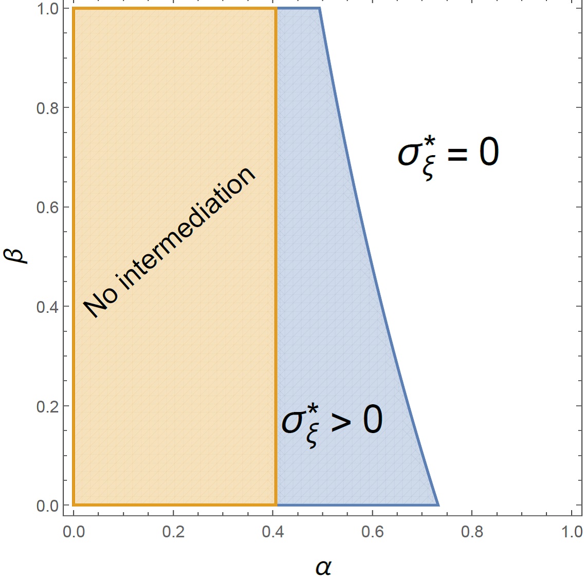
Figure 4: Optimal Additional Noise $(\sigma=1,N=2)$

Proposition 12 (Profitability of Data Intermediation)

Under the optimal data policy, the intermediary’s profits are strictly positive if and only if

$$\alpha>\frac{N(\sqrt{3}+1)-1}{2N\left(N+1\right)-1}\in\left(0,1\right)\text{.}$$

Proof of Proposition 12. Recall that $\alpha$ is the correlation coefficient between $w_{i}$ and $w_{j}.$ Because we have normalized $\mathop{\rm var}\left[w_{i}\right]=1$, under the additive structure, we have $\sigma_{\theta}^{2}=\alpha$ and $\sigma_{\theta_{i}}^{2}=1-\alpha$. To establish the result in the statement, we must then show that the intermediary obtains positive profits if and only if

$$N\left(\sqrt{3}-1\right)\sigma_{\theta}^{2}-\sigma_{\theta_{i}}^{2}>0.$$

When $N\left(\sqrt{3}-1\right)\sigma_{\theta}^{2}<\sigma_{\theta_{i}}^{2}$, we have:

$$R =\frac{3N\sigma_{\theta}^{4}}{8(\sigma_{\theta}^{2}+\sigma_{\varepsilon}^{2})}\left(1-\frac{\sigma_{\theta_{i}}^{2}+\sigma_{\varepsilon_{i}}^{2}}{(N-1)(\sigma_{\varepsilon}^{2}+\sigma_{\theta}^{2})+\sigma_{\varepsilon_{i}}^{2}+\sigma_{\theta_{i}}^{2}}\right)-\frac{(N\sigma_{\theta}^{2}+\sigma_{\theta_{i}}^{2})^{2}}{8N(\sigma_{\theta}^{2}+\sigma_{\varepsilon}^{2})}\left(1-\frac{\sigma_{\theta_{i}}^{2}+\sigma_{\varepsilon_{i}}^{2}}{N(\sigma_{\varepsilon}^{2}+\sigma_{\theta}^{2})+\sigma_{\varepsilon_{i}}^{2}+\sigma_{\theta_{i}}^{2}}\right)$$

$$\leq\left(\frac{3N\sigma_{\theta}^{4}}{8(\sigma_{\theta}^{2}+\sigma_{\varepsilon}^{2})}-\frac{(N\sigma_{\theta}^{2}+\sigma_{\theta_{i}}^{2})^{2}}{8N(\sigma_{\theta}^{2}+\sigma_{\varepsilon}^{2})}\right)\left(1-\frac{\sigma_{\theta_{i}}^{2}+\sigma_{\varepsilon_{i}}^{2}}{N(\sigma_{\varepsilon}^{2}+\sigma_{\theta}^{2})+\sigma_{\varepsilon_{i}}^{2}+\sigma_{\theta_{i}}^{2}}\right)\leq 0.$$

Conversely, when $N\left(\sqrt{3}-1\right)\sigma_{\theta}^{2}>\sigma_{\theta_{i}}^{2}$, we can rewrite $R$ as

$$\frac{A\sigma_{\varepsilon}^{2}+B}{8(N\sigma_{\varepsilon}^{2}+\sigma_{\varepsilon_{i}}^{2}+N\sigma_{\theta}^{2}+\sigma_{\theta_{i}}^{2})(N\sigma_{\varepsilon}^{2}-\sigma_{\varepsilon}^{2}+\sigma_{\varepsilon_{i}}^{2}+N\sigma_{\theta}^{2}-\sigma_{\theta}^{2}+\sigma_{\theta_{i}}^{2})},$$

$$A =(N-1)\left(2N^{2}\sigma_{\theta}^{4}-2N\sigma_{\theta}^{2}\sigma_{\theta_{i}}^{2}-\sigma_{\theta_{i}}^{4}\right)>0.$$

Therefore the intermediary can obtain a positive profit $R$ by setting $\sigma_{\varepsilon}^{2}$ sufficiently large through the addition of correlated noise.   

The optimal level of common noise $\sigma_{\xi}^{\ast}$ is strictly positive when the number of consumers $N$ or the correlation in their willingness to pay $\alpha$ is sufficiently small: if the consumers’ preferences are sufficiently correlated, or if the market is sufficiently large, the intermediary does not add any noise. If the consumers’ fundamentals are not sufficiently correlated, the intermediary makes their signals more correlated with additional common noise $\sigma_{\xi}^{\ast}.$

The additional noise reduces the amount of information procured from consumers and hence the total compensation owed to them. These cost savings come at the expense of lower revenues. In this respect, aggregation and noise serve a common purpose. However, because the intermediary optimally anonymizes the consumers’ signals, the correlation in the supplemental noise terms $\xi$ renders signal $s_{i}$ less valuable on the margin for estimating the average willingness to pay $\bar{w}.$ In other words, the aggregate demand information without consumer $i$’s signal $s_{i}$ is a relatively better predictor of $\bar{w}$ when the intermediary uses common rather than idiosyncratic noise. Therefore, by using common noise exclusively, the intermediary can hold the information sold to the producer constant while reducing the cost of acquiring that information from consumers.

Finally, note that these two elements of information design—aggregation and noise—interact richly with one another. In particular, the value of common noise is deeply linked to that of aggregate data: if the intermediary is restricted to complete (identity-revealing) data sharing, one can show that supplemental idiosyncratic noise is optimal when the consumers’ initial signals $s_{i}$ are sufficiently precise.

References

- [1] \harvarditem[Acquisti, Taylor, and Wagman]Acquisti, Taylor, and Wagman2016actw16 Acquisti, A., C. Taylor, and L. Wagman (2016): “The Economics of Privacy,” Journal of Economic Literature, 54, 442–492.
- [2] \harvarditem[Ali, Lewis, and Vasserman]Ali, Lewis, and Vasserman2019allv19 Ali, S. N., G. Lewis, and S. Vasserman (2019): “Voluntary Disclosure and Personalized Pricing,” Discussion Paper 26592, National Bureau of Economic Research.
- [3] \harvarditem[Aridor, Che, and Salz]Aridor, Che, and Salz2020archsa20 Aridor, G., Y.-K. Che, and T. Salz (2020): “The Economic Consequences of Data Privacy Regulation: Empirical Evidence from GDPR,” Discussion Paper 26900, National Bureau of Economic Research.
- [4] \harvarditem[Arrieta-Ibarra, Goff, Jimenez-Hernandez, Lanier, and Weyl]Arrieta-Ibarra, Goff, Jimenez-Hernandez, Lanier, and Weyl2018agjl18 Arrieta-Ibarra, I., L. Goff, D. Jimenez-Hernandez, J. Lanier, and G. Weyl (2018): “Should We Treat Data as Labor? Moving beyond ”Free”,” American Economic Review Paper and Proceedings, 108, 38–42.
- [5] \harvarditem[Athey, Catalini, and Tucker]Athey, Catalini, and Tucker2017atct17 Athey, S., C. Catalini, and C. Tucker (2017): “The Digital Privacy Paradox: Small Money, Small Costs, Small Talk,” Discussion Paper 23488, National Bureau of Economic Research.
- [6] \harvarditem[Bergemann and Bonatti]Bergemann and Bonatti2011bebo11 Bergemann, D., and A. Bonatti (2011): “Targeting in Advertising Markets: Implications for Offline Vs. Online Media,” Rand Journal of Economics, 42(3), 417–443.
- [7] \harvarditem[Bergemann and Bonatti]Bergemann and Bonatti2019bebo19 Bergemann, D., and A. Bonatti (2019): “Markets for Information: An Introduction,” Annual Review of Economics, 11, 85–107.
- [8] \harvarditem[Bergemann, Brooks, and Morris]Bergemann, Brooks, and Morris2015bebm15 Bergemann, D., B. Brooks, and S. Morris (2015): “The Limits of Price Discrimination,” American Economic Review, 105, 921–957.
- [9] \harvarditem[Choi, Jeon, and Kim]Choi, Jeon, and Kim2019chjk19 Choi, J., D. Jeon, and B. Kim (2019): “Privacy and Personal Data Collection with Information Externalities,” Journal of Public Economics, 173, 113–124.
- [10] \harvarditem[Committee on the Judiciary]Committee on the Judiciary2020house20 Committee on the Judiciary (2020): “Investigation of Competition in Digital Markets,” Discussion paper, United States House of Representatives.
- [11] \harvarditem[Cremèr, de Montjoye, and Schweitzer]Cremèr, de Montjoye, and Schweitzer2019crem19 Cremèr, J., Y.-A. de Montjoye, and H. Schweitzer (2019): “Competition policy for the digital era,” Discussion paper, European Commission.
- [12] \harvarditem[Cummings, Ligett, Pai, and Roth]Cummings, Ligett, Pai, and Roth2016clpr16 Cummings, R., K. Ligett, M. Pai, and A. Roth (2016): “The Strange Case of Privacy in Equilibrium Models,” in ACM-EC (Economics and Computation) 2016.
- [13] \harvarditem[Fainmesser, Galeotti, and Momot]Fainmesser, Galeotti, and Momot2020fagm20 Fainmesser, I., A. Galeotti, and R. Momot (2020): “Digital Privacy,” Discussion paper, Johns Hopkins University.
- [14] \harvarditem[Furman, Coyle, Fletcher, McAules, and Marsden]Furman, Coyle, Fletcher, McAules, and Marsden2019furm19 Furman, J., D. Coyle, A. Fletcher, D. McAules, and P. Marsden (2019): “Unlocking Digital Competition: Report of the Digital Competition Expert Panel,” HM Treasury, United Kingdom.
- [15] \harvarditem[Gradwohl]Gradwohl2017grad17 Gradwohl, R. (2017): “Information Sharing and Privacy in Networks,” in ACM-EC (Economics and Computation) 2017.
- [16] \harvarditem[Ichihashi]Ichihashi2020aichi20 Ichihashi, S. (2020a): “The Economics of Data Externalities,” Discussion paper, Bank of Canada.
- [17] \harvarditem[Ichihashi]Ichihashi2020bichi20aer Ichihashi, S. (2020b): “Online Privacy and Information Disclosure by Consumers,” American Economic Review, 110(2), 569–595.
- [18] \harvarditem[Johnson, Shriver, and Goldberg]Johnson, Shriver, and Goldberg2020joshgo20 Johnson, G., S. Shriver, and S. Goldberg (2020): “Privacy & market concentration: Intended & unintended consequences of the GDPR,” Discussion paper, Boston University Questrom School of Business.
- [19] \harvarditem[Jullien, Lefouili, and Riordan]Jullien, Lefouili, and Riordan2020julr20 Jullien, B., Y. Lefouili, and M. Riordan (2020): “Privacy Protection, Security, and Consumer Retention,” Discussion paper, Toulouse School of Economics.
- [20] \harvarditem[Liang and Madsen]Liang and Madsen2020lima20 Liang, A., and E. Madsen (2020): “Data and Incentives,” Discussion paper, Northwestern University.
- [21] \harvarditem[Lin]Lin2019lin19 Lin, T. (2019): “Valuing Intrinsic and Instrumental Preferences for Privacy,” .
- [22] \harvarditem[Lizzeri]Lizzeri1999lizz99 Lizzeri, A. (1999): “Information Revelation and Certification Intermediaries,” RAND Journal of Economics, 30, 214–231.
- [23] \harvarditem[Loertscher and Marx]Loertscher and Marx2020loma20 Loertscher, S., and L. M. Marx (2020): “Digital monopolies: Privacy protection or price regulation?,” International Journal of Industrial Organization, 71, 1–13.
- [24] \harvarditem[Miklos-Thal and Shaffer]Miklos-Thal and Shaffer2016mish16 Miklos-Thal, J., and G. Shaffer (2016): “Naked Exclusion with Private Offers,” American Economic Journal: Microeconomics, 8, 174–194.
- [25] \harvarditem[Olea, Ortoleva, Pai, and Prat]Olea, Ortoleva, Pai, and Prat2019oopp19 Olea, J. L. M., P. Ortoleva, M. Pai, and A. Prat (2019): “Competing Models,” arXiv preprint arXiv:1907.03809.
- [26] \harvarditem[Posner and Weyl]Posner and Weyl2018powe18 Posner, E. A., and E. G. Weyl (2018): Radical markets: Uprooting capitalism and democracy for a just society. Princeton University Press.
- [27] \harvarditem[Robinson]Robinson1933robi33 Robinson, J. (1933): The Economics of Imperfect Competition. Macmillan, London.
- [28] \harvarditem[Romer]Romer2019romer19 Romer, P. (2019): “A Tax That Could Fix Big Tech,” The New York Times.
- [29] \harvarditem[Schmalensee]Schmalensee1981schm81 Schmalensee, R. (1981): “Output and Welfare Implications of Monopolistic Third-Degree Price Discrimination,” American Economic Review, 71, 242–247.
- [30] \harvarditem[Segal]Segal1999sega99 Segal, I. (1999): “Contracting with Externalities,” Quarterly Journal of Economics, 114, 337–388.
- [31] \harvarditem[Segal and Whinston]Segal and Whinston2000sewh00 Segal, I., and M. Whinston (2000): “Naked Exclusion: Comment,” American Economic Review, 90, 296–309.
- [32] \harvarditem[Stigler Committee on Digital Platforms]Stigler Committee on Digital Platforms2019stig19 Stigler Committee on Digital Platforms (2019): “Final Report,” Discussion paper, Stigler Center for the Study of the Economy and the State.
- [33] \harvarditem[Tang]Tang2019tang19 Tang, H. (2019): “The Value of Privacy: Evidence from Online Borrowers,” Discussion paper, HEC Paris.
- [34] \harvarditem[Taylor]Taylor2004tayl04 Taylor, C. (2004): “Consumer Privacy and the Market for Customer Information,” RAND Journal of Economics, 35, 631–651.
- [35] \harvarditem[Zuboff]Zuboff2019zubo19 Zuboff, S. (2019): The Age of Surveillance Capitalism: The Fight for a Human Future at the New Frontier of Power. Public Affairs, New York.
- [36]