Decoupling Cross-Quadrature Correlations using Passive Operations

Abstract

Quadrature correlations between subsystems of a Gaussian quantum state are fully characterised by its covariance matrix. For example, the covariance matrix determines the amount of entanglement or decoherence of the state. Here, we establish when it is possible to remove correlations between conjugate quadratures using only passive operations. Such correlations are usually undesired and arise due to experimental cross-quadrature contamination. Using the Autonne–Takagi factorisation, we present necessary and sufficient conditions to determine when such removal is possible. Our proof is constructive, and whenever it is possible we obtain an explicit expression for the required passive operation.

I Introduction

The decomposition of Gaussian quantum systems has proven to be a fruitful subject of research. For instance, the textbook examples of Williamson Williamson (1936); Simon et al. (1994) and Braunstein Braunstein (2005) tell us that any Gaussian state can be decomposed through beamsplitters, phase shifters and single-mode squeezers into uncorrelated thermal states. This is useful for designing quantum gates Shiozawa et al. (2018). More generally, instead of demanding the complete diagonalisation of the state, it can also be transformed into another that has specific kinds of correlations. Early examples of this are the Simon and Duan et al. standard forms Simon (2000); Duan et al. (2000): using local squeezing and phase shifts to bring an entangled state into some standard form of correlations. This turned out to be important in advancing our understanding of Gaussian entanglement.

All the transformations above require the use of active operations and bring the state to a form that does not have any cross-quadrature correlations. Active operations are those that require an external source of energy, for example, squeezing, while passive operations are those that do not Weedbrook et al. (2012). Active operations are usually more difficult to implement in a real device compared to passive operations which can be implemented almost free of errors using beamsplitters and phase shifts Reck et al. (1994). When restricted to only passive operations, a generic Gaussian state cannot be diagonalised; it can only be brought to standard forms that remain correlated. There exist conditions with which one can check whether a Gaussian state can be diagonalised by a passive operation Simon et al. (1994); Arvind et al. (1995). These conditions are always satisfied when the Gaussian states are pure Braunstein (2005); Arvind et al. (1995).

Here, instead of requiring the state to be fully diagonalised, we report a necessary and sufficient condition under which the correlations between conjugate quadrature variables can be entirely removed using passive operations only. This is stated in the following theorem.

Theorem 1.

Let $\mathbf{a}=\left[a_{1},\ldots,a_{n},a_{1}^{\dagger},\ldots,a_{n}^{\dagger}\right]$ be a vector collecting the annihilation and creation operators of $n$ modes. Let

$$\mathsf{S}_{jk}=\frac{1}{2}\mathrm{Tr}\left[\rho\left(\mathbf{a}_{j}\mathbf{a}_{k}^{\dagger}+\mathbf{a}_{k}^{\dagger}\mathbf{a}_{j}\right)\right]=\begin{bmatrix}\mathsf{X}&\mathsf{Y}\\ {\mathsf{Y}}^{*}&{\mathsf{X}}^{*}\end{bmatrix}_{jk}$$

be the complex covariances of an $n$-mode Gaussian state $\rho$ having zero mean $\mathrm{Tr}\left[\rho\,\mathbf{a}\right]=0$. Then $\mathsf{S}$ can be brought into a cross-quadrature decorrelated form using passive operations if and only if there exist an Autonne–Takagi factorisation of $\mathsf{Y}$: $\mathsf{Y}=\mathsf{Z}^{\dagger}\mathsf{Y}_{0}\mathsf{Z}^{*}$, and a diagonal matrix $\mathsf{R}$ with entries in $\{1,i\}$ such that $\mathsf{R}^{\dagger}\mathsf{Z}\mathsf{\mathsf{X}}\mathsf{Z}^{\dagger}\mathsf{R}$ is real. Furthermore, the required passive operation is given by $\mathsf{Z}$ up to swapping of quadratures determined by $\mathsf{R}$.

The crux of the theorem is the diagonalisation of $\mathsf{Y}$, which is given to us by the Autonne–Takagi factorisation Autonne (1915); Takagi (1925).

Theorem 2 (Autonne–Takagi factorisation).

Let $\mathsf{Y}$ be a complex symmetric matrix. Then there exists a unitary matrix $\mathsf{Z}$ such that $\mathsf{Y}=\mathsf{Z}^{\dagger}\mathsf{Y}_{0}\mathsf{Z}^{*}$, with $\mathsf{Y}_{0}$ real, non-negative and diagonal.

The diagonal entries of $\mathsf{Y}_{0}$ are the singular values of $\mathsf{Y}$ in any desired order. The uniqueness property of $\mathsf{Z}$ is stated in Appendix A. Essentially, the physical situation of interest is a correlated state with unwanted correlations between some of the conjugate quadratures and we are concerned with the conditions under which these unwanted correlations can be removed using only passive operations. We mean “conjugate quadratures” in a more general sense—any quadrature pairs, $q_{j}$ and $p_{k}$ with $j$ not necessarily equal to $k$ and where $[q_{j},p_{k}]={i\mkern 1.0mu}\delta_{jk}$. In other words, theorem 1 identifies those states that are composed of $q$correlations and $p$ correlations plus passive operations. As a corollary, it also identifies states which cannot be constructed by passive operations on initially uncorrelated, squeezed or otherwise, single modes. The proof of the theorem is constructive in that the required passive operation is obtained whenever it exists. It turns out to be, up to local rotations, just $\mathsf{Z}$ given by the Autonne–Takagi’s factorisation, which is very convenient.

We note that Autonne–Takagi’s factorisation makes its appearance in multimode quantum optics Cariolaro and Pierobon (2016); Arzani et al. (2018) that resembles the approach we have taken here, but there is one important difference—we consider the factorisation of quantum states rather than the decomposition of unitaries for determining supermodes as is the case in multimodal theories.

II Proof of theorem 1

In what follows, we prove Theorem 1. We work with the complex covariance matrix which can be obtained from the quadrature covariance matrix by the change of variables Schumaker and Caves (1985)

$$a_{j}=\frac{q_{j}+{i\mkern 1.0mu}p_{j}}{\sqrt{2}}\;\text{ and }\;a_{j}^{\dagger}=\frac{q_{j}-{i\mkern 1.0mu}p_{j}}{\sqrt{2}}\,.$$ (1)

The reason for working in such a basis is twofold. First, the conjugate quadratures have vanishing correlations if and only if both matrices $\mathsf{X}$ and $\mathsf{Y}$ are real. Second, passive operations take the simple form

$$\begin{bmatrix}\mathsf{E}&0\\ 0&\mathsf{E}^{*}\end{bmatrix}$$

with $\mathsf{E}$ unitary due to the symplectic conditions. A direct calculation shows that the covariance matrix transforms as $\mathsf{E}:(\mathsf{X},\mathsf{Y})\mapsto(\mathsf{E}\mathsf{X}\mathsf{E}^{\dagger},\mathsf{E}\mathsf{Y}\mathsf{E}^{\intercal})$ under passive operations, whence it follows that the problem of decoupling conjugate variables is reduced to finding a unitary matrix $\mathsf{E}$ such that $\mathsf{E}\mathsf{X}\mathsf{E}^{\dagger}$ and $\mathsf{E}\mathsf{Y}\mathsf{E}^{\intercal}$ are simultaneously real. We can now proceed to prove the main result.

Proof: Forward direction.

Suppose $\mathsf{S}$ is the covariance matrix of a state $\rho$ with cross-quadrature correlations which can be removed by a passive operation $\mathsf{Q}$. In other words, after applying $\mathsf{Q}$, the cross-quadrature correlations $\left\{q_{j},p_{k}\right\}=0$, where to simplify notations, we use $\left\{q_{j},p_{k}\right\}$ to mean $\frac{1}{2}\text{Tr}\left[\rho(q_{j}p_{k}+p_{k}q_{j})\right]$. In the complex representation, denoting the transformed matrix as $\mathsf{X}_{1}=\mathsf{Q}\mathsf{X}\mathsf{Q}^{\dagger}$ and $\mathsf{Y}_{2}=\mathsf{Q}\mathsf{Y}\mathsf{Q}^{\intercal}$, the transformed covariance matrix has entries

$$[\mathsf{X}_{1}]_{jk}=\left\{a_{j},a_{k}^{\dagger}\right\} =\frac{\left\{q_{j},q_{k}\right\}}{2}+\frac{\left\{p_{j},p_{k}\right\}}{2}$$

$$[\mathsf{Y}_{2}]_{jk}=\left\{a_{j},a_{k}\right\} =\frac{\left\{q_{j},q_{k}\right\}}{2}-\frac{\left\{p_{j},p_{k}\right\}}{2}$$

which are real. Since $\mathsf{Y}_{2}$ is a real symmetric matrix, it has a spectral decomposition $\mathsf{Y}_{2}=\mathsf{R}_{1}^{\intercal}\mathsf{Y}_{1}\mathsf{R}_{1}$ Horn and Johnson (2012), where $\mathsf{R}_{1}$ is a real orthogonal matrix and $\mathsf{Y}_{1}$ is a real (but not necessarily positive) diagonal matrix the entries of which are the eigenvalues of $\mathsf{Y}_{2}$. To obtain the Autonne–Takagi decomposition, consider a passive unitary (but not necessarily real) transformation $\mathsf{R}:(a_{j},a_{j}^{\dagger})\mapsto(ia_{j},-ia_{j}^{\dagger})$ on $\mathsf{Y}_{1}$ for every $j\in J$ where $J$ is the set containing all indices $j$ for which $[\mathsf{Y}_{1}]_{jj}$ is negative. This corresponds to a rotation of the quadratures $\mathsf{R}:(q_{j},p_{j})\mapsto(p_{j},-q_{j})$ for $j\in J$. In matrix form, $\mathsf{R}$ is diagonal with entries

$$[\mathsf{R}]_{jk}=\begin{cases}1&\text{for }j=k\notin J\,,\\ i&\text{for }j=k\in J\\ 0&\text{for }j\neq k\,.\end{cases}$$

Applying this to $\mathsf{Y}_{1}$ brings it to a non-negative diagonal matrix $\mathsf{Y}_{0}=\mathsf{R}\mathsf{Y}_{1}\mathsf{R}^{\intercal}$ since

$$\mathsf{R}:\left\{a_{j},a_{j}\right\}\mapsto\begin{cases}-\left\{a_{j},a_{j}\right\}&\text{ for }\left\{a_{j},a_{j}\right\}<0\,,\\ \left\{a_{j},a_{j}\right\}&\text{ for }\left\{a_{j},a_{j}\right\}\geq 0\,.\end{cases}$$

Putting everything together, we arrive at the Autonne–Takagi decomposition of $\mathsf{Y}$ as

$$\mathsf{Y}=\underbrace{\mathsf{Q}^{\dagger}\mathsf{R}_{1}^{\intercal}\mathsf{R}^{\dagger}}_{\mathsf{Z}^{\dagger}}\mathsf{Y}_{0}\underbrace{\mathsf{R}^{*}\mathsf{R}_{1}\mathsf{Q}^{*}}_{\mathsf{Z}^{*}}\,.$$

Then $\mathsf{X}$ transforms as

$$\mathsf{Z}\mathsf{X}\mathsf{Z}^{\dagger} =\mathsf{R}\mathsf{R}_{1}^{*}\mathsf{Q}\mathsf{X}\mathsf{Q}^{\dagger}\mathsf{R}_{1}^{\intercal}\mathsf{R}^{\dagger}$$

$$=\mathsf{R}\underbrace{\mathsf{R}_{1}^{*}\mathsf{X}_{1}\mathsf{R}_{1}^{\intercal}}_{\mathsf{X}_{0}}\mathsf{R}^{\dagger}\,,$$

where $\mathsf{X}_{0}$ is a real (symmetric) matrix since both $\mathsf{X}_{1}$ and $\mathsf{R}_{1}$ are real. This implies $\mathsf{R}^{\dagger}\mathsf{Z}\mathsf{X}\mathsf{Z}^{\dagger}\mathsf{R}$ is real which completes the proof. ∎

Proof: Reverse direction.

Let $\mathsf{Z}$ be the unitary matrix in the Autonne–Takagi factorisation of $\mathsf{Y}$: $\mathsf{Y}=\mathsf{Z}^{\dagger}\mathsf{Y}_{0}\mathsf{Z}^{*}$ and $\mathsf{R}$ be a diagonal matrix with entries in $\{1,i\}$ such that $\mathsf{R}^{\dagger}\mathsf{Z}\mathsf{X}\mathsf{Z}^{\dagger}\mathsf{R}$ is real. The passive transformation $\mathsf{R}^{\dagger}\mathsf{Z}$ results in $\mathsf{R}^{\dagger}\mathsf{Z}:(\mathsf{X},\mathsf{Y})\mapsto(\mathsf{R}^{\dagger}\mathsf{Z}\mathsf{X}\mathsf{Z}^{\dagger}\mathsf{R},\mathsf{R}^{\dagger}\mathsf{Z}\mathsf{Y}\mathsf{Z}^{\intercal}\mathsf{R}^{*})$. The first term is real by assumption. The second term

$$\mathsf{R}^{\dagger}\mathsf{Z}\mathsf{Y}\mathsf{Z}^{\intercal}\mathsf{R}^{*}=\mathsf{R}^{\dagger}\mathsf{Z}\mathsf{Z}^{\dagger}\mathsf{Y}_{0}\mathsf{Z}^{*}\mathsf{Z}^{\intercal}\mathsf{R}^{*}=\mathsf{R}^{\dagger}\mathsf{Y}_{0}\mathsf{R}^{*}$$

is also real since $\mathsf{Y}_{0}$ is a real diagonal matrix. When $\mathsf{X}$ and $\mathsf{Y}$ are simultaneously real, it follows from direct substitution that the quadrature covariance matrix has no cross-quadrature correlations. ∎

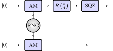
Figure 1: The output state with quadrature covariance matrix given by (2) has cross-quadrature correlations that cannot be removed by passive operations. AM: Amplitude modulator. RNG: Gaussian random number generator with variance $1/2$. $R(\frac{\pi}{4})$: $\pi/4$ phase shifter. SQZ: $3\text{\,}\mathrm{dB}$ squeezer.

What does this mean? It means that we have a way of testing if the correlations between conjugate variables can be removed—diagonalise $\mathsf{Y}$ to obtain the matrix $\mathsf{Z}$ using the Autonne–Takagi factorisation and subsequently compute $\mathsf{Z}\mathsf{X}\mathsf{Z}^{\dagger}$. If $\mathsf{Y}$ is a full-rank matrix with non-degenerate eigenvalues and $\mathsf{Z}\mathsf{X}\mathsf{Z}^{\dagger}$ cannot be transformed to a real matrix by a diagonal matrix $\mathsf{R}$, then the correlations cannot be decoupled. This is certainly the case if $\mathsf{Z}\mathsf{X}\mathsf{Z}^{\dagger}$ has any entries that are neither real nor purely imaginary. On the other hand, if all the entries of $\mathsf{Z}\mathsf{X}\mathsf{Z}^{\dagger}$ are real, then $\mathsf{Z}$ is the passive operation that we are after. If some entries are purely imaginary then in addition to $\mathsf{Z}$, additional local rotations $\mathsf{R}$ are required. If $\mathsf{Y}$ is singular or has degenerate eigenvalues, then we have some freedom in choosing $\mathsf{Z}$ to make the entries of $\mathsf{R}^{\dagger}\mathsf{Z}\mathsf{X}\mathsf{Z}^{\dagger}\mathsf{R}$ real.

When $\mathsf{S}$ corresponds to a pure state, the matrix $\mathsf{Z}$ gives the passive operation required to create it from a product of independent squeezed states. However, if $\mathsf{S}$ is mixed, our result implies that it is sometimes impossible to create by passive operations on any independent states, or even on states possessing only $q$ correlations and $p$ correlations. One example is the state with quadrature covariance matrix

$$\mathcal{S}=\frac{1}{2}\begin{bmatrix}3&0.5&1&0\\ 0.5&0.75&0.5&0\\ 1&0.5&2&0\\ 0&0&0&1\end{bmatrix}$$ (2)

which can be created by the scheme in Fig 1. The squeezing operation “locks in” the cross-quadrature correlations and makes it impossible to be removed using passive operations only.

III Two-mode example

We illustrate our result by working through an example. Consider a two-mode Gaussian state having the following quadrature covariance matrix

$$\mathcal{S}=\begin{bmatrix}m&0&c&0\\ 0&m&0&-c\\ c&0&n&s\\ 0&-c&s&n\end{bmatrix}$$

with all $m$, $n$, $c$ and $s$ positive. We want to determine if this state can be brought into a cross-quadrature decorrelated form. The basis transformation (1) represented by the unitary matrix

$$\mathcal{L}=\frac{1}{\sqrt{2}}\begin{bmatrix}1&{i\mkern 1.0mu}&0&0\\ 0&0&1&{i\mkern 1.0mu}\\ 1&-{i\mkern 1.0mu}&0&0\\ 0&0&1&-{i\mkern 1.0mu}\end{bmatrix}$$

transforms the quadrature covariance matrix into the complex covariance matrix

$$\mathsf{S}=\mathcal{L}\mathcal{S}\mathcal{L}^{\dagger}=\begin{bmatrix}m&0&0&c\\ 0&n&c&{i\mkern 1.0mu}s\\ 0&c&m&0\\ c&-{i\mkern 1.0mu}s&0&n\end{bmatrix}\,,$$

which identifies $\mathsf{X}$ and $\mathsf{Y}$ as

$$\mathsf{X}=\begin{bmatrix}m&0\\ 0&n\end{bmatrix}\;\text{ and }\mathsf{Y}=\begin{bmatrix}0&c\\ c&{i\mkern 1.0mu}s\end{bmatrix}\,.$$

The Autonne–Takagi factorisation of $\mathsf{Y}=\mathsf{Z}^{\dagger}\mathsf{Y}_{0}\mathsf{Z}^{*}$ is given by

$$\mathsf{Z} =e^{i\pi/4}\begin{bmatrix}-i\sqrt{t}&\sqrt{1-t}\\ \sqrt{1-t}&-i\sqrt{t}\end{bmatrix}$$

and

$$\mathsf{Y}_{0} =\frac{1}{2}\begin{bmatrix}\sqrt{4c^{2}+s^{2}}-s&0\\ 0&\sqrt{4c^{2}+s^{2}}+s\end{bmatrix}$$

with $t=(1+s/\sqrt{4c^{2}+s^{2}})/2$. This results in

$$\mathsf{Z}\mathsf{X}\mathsf{Z}^{\dagger}=\begin{bmatrix}n(1-t)+mt&-{i\mkern 1.0mu}\sqrt{t(1-t)}(m-n)\\ {i\mkern 1.0mu}\sqrt{t(1-t)}(m-n)&nt+m(1-t)\end{bmatrix}$$

which has entries that are all real or purely imaginary, and is transformed to a real matrix by

$$\mathsf{R}=\begin{bmatrix}1&0\\ 0&{i\mkern 1.0mu}\end{bmatrix}$$

so that finally we have

$$\mathsf{R}^{\dagger}\mathsf{Z}\mathsf{X}\mathsf{Z}^{\dagger}\mathsf{R}=\begin{bmatrix}n(1-t)+mt&\sqrt{t(1-t)}(m-n)\\ \sqrt{t(1-t)}(m-n)&nt+m(1-t)\end{bmatrix}\,.$$

This means that the state $\mathsf{S}$ can be brought to a cross-quadrature decorrelated form and the passive operation that does this is $\mathsf{R}^{\dagger}\mathsf{Z}$. This can be factorised as

$$\mathsf{R}^{\dagger}\mathsf{Z}=\begin{bmatrix}e^{{i\mkern 1.0mu}\pi/4}&0\\ 0&e^{-{i\mkern 1.0mu}3\pi/4}\end{bmatrix}\begin{bmatrix}\sqrt{t}&\sqrt{1-t}\\ -\sqrt{1-t}&\sqrt{t}\end{bmatrix}\begin{bmatrix}e^{-{i\mkern 1.0mu}\pi/2}&0\\ 0&1\end{bmatrix}$$

which is realised by a beamsplitter of transmissivity $t$ and three phase shifts: $\pi/4$ and $-3\pi/4$ at the outputs and $-\pi/2$ at the input port.

The expert reader might have recognised that the state $\mathsf{S}$ can in fact be cross-quadrature decorrelated through the simpler transformation

$$\mathsf{R}^{\dagger}\mathsf{Z}=\begin{bmatrix}e^{{i\mkern 1.0mu}\pi/4}&0\\ 0&e^{-{i\mkern 1.0mu}\pi/4}\end{bmatrix}$$

requiring just two phase shifts. This shows that when it is possible to decorrelate the conjugate quadratures the procedure we presented is not the only way to do so. The condition that $\mathsf{Y}$ be diagonalised can be relaxed—all we need to decouple $q$ and $p$ is for $\mathsf{Y}$ to be transformed into a real matrix after applications of the passive operation—this real matrix need not be diagonal or non-negative. In terms of implementations, this would mean that the required operation might be simpler, for instance we can do away with the beamsplitter in the example considered.

IV Discussions

An immediate application theorem 1 is to the calculation of the “squeezing of formation” Idel et al. (2016). This quantity measures how much squeezing is required to create a given state and indicates the degree of nonclassicality of the state. Squeezing of formation is invariant under passive operations because these transformations do not require any squeezing. This means that the result of this paper can be used to simplify complicated states to a form in which the squeezing of formation can be directly calculated. For example, a brute force computation of the squeezing of formation for a two-mode Gaussian state involves an optimisation over six free parameters. However, by first transforming the state to a quadrature-decorrelated form, if it is possible, this computation reduces to a simple one parameter optimisation problem Tserkis et al. (2020).

There is also an interesting connection with the generation of cluster states. A cluster state has multiple quantum modes with correlations between each mode Menicucci et al. (2006); Raussendorf and Briegel (2001); Raussendorf et al. (2003). Many of these can be shown to possess correlations only between the $q$’s and between the $p$’s, such as the two-dimensional square cluster. However, in real devices for generating cluster states there are imperfections which give rise to correlations between $q$ and $p$. This implies that our result might be useful for identifying if an ideal cluster state can be recovered using only passive operations.

What can be said about a state with cross-quadrature correlations which cannot be removed by passive operations? While most theoretical work on Gaussian quantum information consider cross-quadrature decorrelated states, almost every state realised experimentally would have some cross-quadrature correlations that cannot be decoupled using only passive operations. However, if we are also allowed to add correlated noise in the form of random Gaussian quadrature displacements, then any state can be cross-quadrature decorrelated. One obvious question is then the following: what is the least amount of noise required to achieve such decorrelation?

Appendix A Uniqueness of Autonne–Takagi decomposition

For completeness, this Appendix recalls the uniqueness properties of the Autonne–Takagi decomposition. See for example the textbook by Horn and Johnson (2012) for proofs.

Let $\mathsf{Y}$ be an $n\times n$ complex symmetric matrix of rank $r$. Let $\lambda_{1},\ldots,\lambda_{d}$ be the distinct positive singular values of $\mathsf{Y}$, in any given order with respective multiplicities $n_{1},\ldots,n_{d}$. Let $\mathsf{Y}_{0}=\lambda_{1}\mymathbb{1}_{n_{1}}\oplus\ldots\oplus\lambda_{d}\mymathbb{1}_{n_{d}}\oplus\mymathbb{0}_{n-r}$; the zero block is missing if $\mathsf{Y}$ is nonsingular. Let $\mathsf{U}$ and $\mathsf{V}$ be unitary. Then the Autonne–Takagi decomposition of $\mathsf{Y}$: $\mathsf{Y}=\mathsf{U}\mathsf{Y_{0}}\mathsf{U}^{\intercal}=\mathsf{V}\mathsf{Y_{0}}\mathsf{V}^{\intercal}$ if and only if $\mathsf{V}=\mathsf{UQ}$, with $\mathsf{Q}=\mathsf{Q}_{1}\oplus\ldots\oplus\mathsf{Q}_{d}\oplus\mathsf{W}$ where each $\mathsf{Q}_{j}$ is an $n_{j}\times n_{j}$ real orthogonal matrix and $\mathsf{W}$ is an $(n-r)\times(n-r)$ unitary matrix. If the singular values of $\mathsf{Y}$ are distinct (that is, if $d\geq n-1$), then $\mathsf{V}=\mathsf{UD}$, in which $\mathsf{D}=\text{diag}(d_{1},\ldots,d_{n})$ with $d_{j}=\pm 1$ for each $j=1,\ldots,n-1$. The last entry $d_{n}=e^{i\theta}$ if $\mathsf{Y}$ is singular ($d=n-1$), otherwise $d_{n}=\pm 1$ if $\mathsf{Y}$ is nonsingular ($d=n$).

References

- Williamson (1936) J. Williamson, Amer. J. Math. 58, 141 (1936).
- Simon et al. (1994) R. Simon, N. Mukunda, and Biswadeb Dutta, Phys. Rev. A 49, 1567–1583 (1994).
- Braunstein (2005) S. L. Braunstein, Phys. Rev. A 71, 055801 (2005).
- Shiozawa et al. (2018) Y. Shiozawa, J. Yoshikawa, S. Yokoyama, T. Kaji, K. Makino, T. Serikawa, R. Nakamura, S. Suzuki, S. Yamazaki, W. Asavanant, S. Takeda, P. van Loock, and A. Furusawa, Phys. Rev. A 98, 052311 (2018).
- Simon (2000) R. Simon, Phys. Rev. Lett. 84, 2726–2729 (2000).
- Duan et al. (2000) L. M. Duan, G. Giedke, J. I. Cirac, and P. Zoller, Phys. Rev. Lett. 84, 2722 (2000).
- Weedbrook et al. (2012) Christian Weedbrook, Stefano Pirandola, Raúl García-Patrón, Nicolas J. Cerf, Timothy C. Ralph, Jeffrey H. Shapiro, and Seth Lloyd, Rev. Mod. Phys. 84, 621–669 (2012).
- Reck et al. (1994) Michael Reck, Anton Zeilinger, Herbert J. Bernstein, and Philip Bertani, Phys. Rev. Lett. 73, 58–61 (1994).
- Arvind et al. (1995) Arvind, B Dutta, N Mukunda, and R Simon, Pramana 45, 471–497 (1995).
- Autonne (1915) L. Autonne, Ann. Univ. Lyon 38, 1 (1915).
- Takagi (1925) T. Takagi, Japan. J. Math. 1, 83 (1925).
- Cariolaro and Pierobon (2016) G. Cariolaro and G. Pierobon, Phys. Rev. A 94, 062109 (2016).
- Arzani et al. (2018) F. Arzani, C. Fabre, and N. Treps, Phys. Rev. A 97, 033808 (2018).
- Schumaker and Caves (1985) Bonny L. Schumaker and Carlton M. Caves, Phys. Rev. A 31, 3093–3111 (1985).
- Horn and Johnson (2012) Roger A Horn and Charles R Johnson, Matrix analysis (Cambridge university press, 2012).
- Idel et al. (2016) M. Idel, D. Lercher, and M. M. Wolf, J. Phys. A: Math. Theor. 49, 445304 (2016).
- Tserkis et al. (2020) Spyros Tserkis, Jayne Thompson, Austin P. Lund, Timothy C. Ralph, Ping Koy Lam, Mile Gu, and Syed M. Assad, (2020), arXiv:2004.13948 [quant-ph] .
- Menicucci et al. (2006) N. C. Menicucci, P. van Loock, M. Gu, C. Weedbrook, T. C. Ralph, and M. A. Nielsen, Phys. Rev. Lett. 97, 110501 (2006).
- Raussendorf and Briegel (2001) R. Raussendorf and H. J. Briegel, Phys. Rev. Lett. 86, 5188 (2001).
- Raussendorf et al. (2003) R. Raussendorf, D. E. Browne, and H. J. Briegel, Phys. Rev. A 68, 022312 (2003).