Probing Compactified Extra Dimensions with Gravitational Waves

Abstract

We study the effect of compact extra dimensions on the gravitational wave luminosity and waveform. We consider a toy model, with a compactified fifth dimension, and matter confined on a brane. We work in the context of five dimensional ($5d$) general relativity, though we do make connections with the corresponding Kaluza-Klein effective $4d$ theory. We show that the luminosity of gravitational waves emitted in $5d$ gravity by a binary with the same characteristics (same masses and separation distance) as a $4d$ binary is 20.8% less relative to the $4d$ case, to leading post-Newtonian order. The phase of the gravitational waveform differs by 26% relative to the $4d$ case, to leading post-Newtonian order. Such a correction arises mainly due to the coupling between matter and dilaton field in the effective $4d$ picture and agrees with previous calculations when we set black holes’ scalar charges to be those computed from the Kaluza-Klein reduction. The above corrections to the waveform and the luminosity are inconsistent with the gravitational-wave and binary pulsar observations and they thus effectively rule out the possibility of such a simple compactified higher dimensions scenario. We also comment on how our results change if there are several compactified extra dimensions, and show that the discrepancy with $4d$ general relativity only increases.

I Introduction

Recent discoveries of gravitational waves have opened a new window for testing general relativity (GR), especially in the strong/dynamical field regime Abbott et al. (2016a); Yunes et al. (2016); Abbott et al. (2016b); Abbott et al. (2019a); Abbott et al. (2019b); Berti et al. (2018a, b), in a way which is complementary to other tests including solar system experiments Will (1993, 2006), binary pulsars Stairs (2003); Wex (2014) and cosmological observations Jain and Khoury (2010); Koyama (2016). Gravitational wave events have been used to probe the fundamental pillars of GR, such as the equivalence principle, Lorentz/parity invariance and massless gravitons Yunes et al. (2016).

One fundamental aspect of gravity that is important to probe is the presence of extra dimensions motivated by e.g. string theory. For example, in flat $D$-dimensional (non-compact) spacetime, gravitational waves decay with distance travelled as $1/R^{(D-2)/2}$ Cardoso et al. (2003). This fact has been used to measure $D$ with gravitational wave observations Pardo et al. (2018); Abbott et al. (2019a). One can also use tidal deformabilities of compact objects to probe extra dimensions. In $4d$ GR tidal deformabilities vanish for non-rotating black holes, but they do not for higher dimensional black holes Kol and Smolkin (2012); Cardoso et al. (2019).

In this paper we consider gravitational waves in a $5d$ spacetime, with the fifth dimension being compactified on a circle and with the matter constrained on a brane. We work in $5d$ GR rather than in the context of the effective Einstein-Maxwell-dilaton $4d$ theory (considered in  Hirschmann et al. (2018); Julié (2018a, b); Khalil et al. (2018)) which arises from performing a Kaluza-Klein reduction of the $5d$ theory. Our motivation is two-fold. First motivation is simplicity: it is easier to work with a single field (the metric) than a collection of fields. Also, by not performing the Kaluza-Klein reduction (which assumes that fields are independent of the compactified dimension) allows us to account for the effect of the massive fluctuations that arise when integrating out the compact dimension. By working directly in higher-dimensional GR theory we are also able to generalize the $5d$ results to an arbitrary number of compactified extra dimensions. Second, we hope that our $5$d analysis will be useful to assess the effect of the extra dimensions on gravitational wave detection when considering other paradigms for the geometry of the extra dimensions, e.g. Randall-Sundrum (RS) models.

Gravitational waves in higher dimensional spacetimes with compactified or warped extra dimensions have been studied in the literature. Kaluza-Klein compactification leads to an extra scalar polarization mode(s) (the breathing mode) plus massive Kaluza-Klein modes, whose frequencies are typically much higher than what can be probed with ground-based detectors Andriot and Lucena Gómez (2017); Andriot and Tsimpis (2019). Such Kaluza-Klein modes also create a stochastic gravitational wave background Kwon et al. (2019) and modify the quasinormal modes after mergers Toshmatov et al. (2016); Chakraborty et al. (2018). Black hole and neutron star tidal deformabilities have been computed within braneworld models and have been applied to GW170817 to constrain the brane tension Chakravarti et al. (2019a, b). In the RS-II braneworld model Randall and Sundrum (1999), black holes may evaporate classically Emparan et al. (2002); Tanaka (2003), which changes the orbital evolution of binary black holes and further modifies the waveform from that in $4d$ GR. This fact has been applied to the GW events, such as GW150914, to place bounds on the size of the extra dimension Yunes et al. (2016), though such bounds are much weaker than those coming from table-top experiments Adelberger et al. (2007); Kapner et al. (2007). Lastly, given that gravitational waves can propagate in the higher dimensional bulk while electromagnetic waves are constrained on a brane, one can compare the propagation of such two waves to probe the extra dimensions Caldwell and Langlois (2001); Abdalla et al. (2002a, b); Abdalla and Cuadros-Melgar (2003); Abdalla et al. (2004), which has been applied to GW170817 Yu et al. (2017); Visinelli et al. (2018); Yu et al. (2019); Lin et al. (2020). Again, these bounds on the extra dimension size are much weaker than those from table-top experiments.

Our paper is organized as follows. In section II we present our conventions, notations and general framework. In section III, we extract the compactified $5d$ Newtonian potential and the modified Kepler’s law for a binary at a fixed position in the extra dimension. In section IV we review the Kaluza-Klein reduction of the $5d$ theory and point out that $5d$ matter, when seen from a $4d$ perspective is non-minimally coupled. Section V contains our main result, namely the form of the gravitational waves sourced by the $5d$ binary. In section VI we extract the luminosity of the gravitational waves, and in section VII we compute the phase of the gravitational waveform as predicted by the compactified $5d$ model, and compare it with observations. Throughout the paper we give generalizations of our formulae in the case of a comapctified $D$-dimensional spacetime, with four non-compact dimensions. We conclude in section VIII. We relegate some of the more technical details to appendices.

II Set-up

We will consider point-like mass sources in some higher-dimensional spacetime, and we will investigate their effect on the spacetime geometry and on the emission of gravitational waves from binaries, in perturbation theory.

To this end we will compute the metric perturbation $\tilde{h}_{\mu\nu}$ by direct integration of Einstein’s equations and not from the quadrupole formula as it is customary, because the quadruple formula actually fails when there is a compactified dimension. The reason for this is that the validity of quadrupole formula relies on integration by parts. When the spatial coordinates are non-compact, the boundary terms which accompany the integration by parts are zero. However, when there are compactified extra dimensions, there are non-zero boundary terms, which are not straightforward to evaluate and which will contribute, in addition to the usual quadrupole integral. Please see Appendix A for the modified expression.

Thus, we need to solve the metric perturbation directly from the Einstein equations. We will use the relaxed Einstein equations in the harmonic gauge  Pati and Will (2000).

For simplicity in most of this paper we will consider a five-dimensional ($5d$) spacetime with coordinates $x^{M}$, with four noncompact dimensions $x^{\mu}$ and a fifth dimension, $x^{5}=w$, compactified on a circle of radius ${\mathcal{R}}$, though we will occasionally point out how our results change in the case of additional compactified extra dimensions:

$$x^{M}=(x^{\mu},x^{5},\dots)=(t,\vec{x},w,\dots)\sim(t,\vec{x},w+2\pi\mathcal{R},\dots),\qquad\,M=0,1,2,3,5,\dots D.$$ (1)

We further denote the spatial coordinates by

$$x^{I}=(\vec{x},w,\dots)=(x,y,z,w,\dots),\qquad I=1,2,3,5\dots D\,,$$ (2)

and the spatial non-compact coordinates by

$$x^{i}=(x,y,z),\qquad i=1,2,3\,.$$ (3)

We set the speed of light to $c=1$.

Let us consider a perturbation of the flat spacetime

$$h_{MN}\equiv g_{MN}-\eta_{MN}\,,\qquad\eta_{MN}={\rm diag}(-1,1,1,1,1,\dots),$$ (4)

and let us also define

$$\tilde{h}^{MN}\equiv\eta^{MN}-\tilde{g}^{MN}\,\qquad\tilde{g}^{MN}\equiv\sqrt{-g}g^{MN},$$ (5)

where $(g)$ is the determinant of the metric $g_{MN}.$ As advertised, we take $\tilde{h}^{MN}$ to satisfy the Lorenz, or de Donder, or harmonic gauge condition:

$$\partial_{M}\tilde{h}^{MN}=0.$$ (6)

To linear order in $h_{MN}$, $\tilde{h}_{MN}$ reduces to the usual trace-reversed metric perturbation:

$$\tilde{h}_{MN}\simeq h_{MN}-\frac{1}{2}h\,\eta_{MN}.$$ (7)

Then, the relaxed Einstein equations state Pati and Will (2000)

$$\square\tilde{h}^{MN}=-16\pi G^{(D)}\tau^{MN}\,,$$ (8)

where $G^{(D)}$ is the gravitational constant in the $D$-dimensional spacetime, $\square=\partial_{M}\partial_{N}\eta^{MN}$, and where $\tau^{MN}$ is given by

$$\tau^{MN}=(-g)(T^{MN}+t^{MN}_{\rm{LL}})+\frac{1}{16\pi G^{(5)}}\bigg{(}{\tilde{h}^{MP}}{}_{,Q}\,{\tilde{h}^{NQ}}{}_{,P}-\tilde{h}^{PQ}{\tilde{h}^{MN}}{}_{,PQ}\bigg{)}\,.$$ (9)

Lastly, $T^{MN}$ is the matter energy-momentum tensor while $t^{MN}_{\rm{LL}}$ is the Landau-Lifshitz  Landau and Lifschits (1975) gravitational energy-momentum pseudo-tensor. In a $D-$dimensional spacetime we have  Yoshino and Shibata (2009)

$$16\pi G^{(D)}(-g)t^{MN}_{\rm{LL}} =\tilde{g}\indices{{}^{M}{}^{N}_{,P}}\tilde{g}\indices{{}^{P}{}^{Q}_{,Q}}-\tilde{g}\indices{{}^{M}{}^{P}_{,P}}\tilde{g}\indices{{}^{N}{}^{Q}_{,Q}}+\frac{1}{2}g^{MN}g_{PQ}\tilde{g}\indices{{}^{P}{}^{R}_{,S}}\tilde{g}\indices$$

$$-\left(g^{MP}g_{QR}\tilde{g}\indices{{}^{NR}_{,S}}\tilde{g}\indices{{}^{QS}_{,P}}+g^{NP}g_{QR}\tilde{g}^{MR}{}_{,S}\tilde{g}\indices{{}^{QS}_{,P}}\right)+g_{PQ}g^{RS}\tilde{g}\indices{{}^{MP}_{,R}}\tilde{g}\indices{{}^{NQ}_{,S}}$$

$$+\frac{1}{4(D-2)}\left(2g^{MP}g^{NQ}-g^{MN}g^{PQ}\right)\left[(D-2)g_{RS}g_{R^{\prime}S^{\prime}}-g_{RR^{\prime}}g_{SS^{\prime}}\right]\tilde{g}\indices{{}^{RR^{\prime}}_{,P}}\tilde{g}\indices{{}^{SS^{\prime}}_{,Q}}\,.$$ (10)

From the relaxed Einstein equations (8) and the harmonic gauge condition (6) it is easy to see that $\tau^{MN}$ obeys the conservation law

$$\partial_{M}\tau^{MN}=\partial_{M}\bigg{(}(-g)(T^{MN}+t^{MN}_{\rm{LL}})\bigg{)}=0\,.$$ (11)

III Modified Kepler’s Law

Let us first consider the scenario where there is one extra non-compact spatial dimension. Thus $D=5$, the background is flat, and we assume that there is one matter source which is point-like, of mass $m$, at rest. Then, the energy-momentum tensor is

$$T^{MN}(x^{\mu},w)=m\delta^{M0}\delta^{N0}\delta^{3}(\vec{x})\delta(w).$$ (12)

The only non-trivial linearized metric fluctuation is $\tilde{h}_{\rm T}^{00}$, and it satisfies

$$\square\tilde{h}_{\rm T}^{00}=-16\pi G^{(5)}T^{00}\,,$$ (13)

where $G^{(5)}$ is the gravitational constant in $5d$. The solution is

$$\tilde{h}^{00}_{\rm T}(\vec{x},w)=\frac{4G^{(5)}m}{\pi(R^{2}+w^{2})}\,,\qquad R^{2}\equiv\vec{x}^{2}=x^{2}+y^{2}+z^{2}.$$ (14)

The $5d$ linearized metric fluctuation $h_{\rm T}^{00}=(2/3)\tilde{h}_{\rm T}^{00}$ corresponds to a Newtonian potential

$$V^{(5)}(R,w)=-{\frac{4}{3}}\frac{G^{(5)}m}{\pi(R^{2}+w^{2})}\,.$$ (15)

If the extra dimension is not flat, but compact, with an identification $w\sim w+2\pi\mathcal{R}$, an observer sees a mass $m$ at every $w=2n\pi\mathcal{R}$, where $\mathcal{R}$ is the radius of compactification and $n\in\mathbb{Z}$ Zwiebach (2006). Summing over all such sources, the resulting linearized metric fluctuation $\tilde{h}_{\rm T}^{00}$ is periodic $\tilde{h}^{00}_{\rm T}(\vec{x},w)\sim\tilde{h}^{00}_{\rm T}(\vec{x},w+2\pi n\mathcal{R})$:

$$\tilde{h}^{00}_{\rm T}(t,\vec{x},w)=\frac{4G^{(5)}m}{\pi}\sum_{n=-\infty}^{\infty}\frac{1}{\vec{x}^{2}+(w-2n\pi\mathcal{R})^{2}}\,,$$ (16)

and, correspondingly, the Newtonian gravitational potential is given by

$$V^{(5,c)}(\vec{x},w)=-{\frac{4}{3}}\frac{G^{(5)}m}{\pi}\sum_{n=-\infty}^{\infty}\frac{1}{R^{2}+(w-2n\pi\mathcal{R})^{2}}\,.$$ (17)

If the observers are located at the same $w$ coordinate as the source (think of the matter source and observer living on the same brane at $w=0$, and ignore for simplicity the backreaction of the brane on the geometry) then we are interested in $V^{(5,c)}(\vec{x},w{=}0)$. Setting $w=0$ and evaluating the sum over $n$ in (17) yields

$$V^{(5,c)}(\vec{x},w{=}0)=-{\frac{4}{3}}\frac{G^{(5)}m}{lR}\coth\left(\frac{\pi R}{l}\right)=-\frac{1}{3}\tilde{h}_{\rm T}^{00}(t,\vec{x},w{=}0)\,,$$ (18)

where

$$l=2\pi\mathcal{R}\,$$ (19)

denotes the length of the compactified extra dimension. For a generalization of (18) to the case when the observer and the source are located at different positions in the compact dimension, please see Appendix B.

There are two useful limits of (18): one is the decompactification limit, when $l\gg R$, and the other is the opposite, with $l\ll R$. In the first case, the Newtonian potential assumes the form of a $4d$ non-compact space

$$V^{(5,c)}(R,w{=}0)=-{\frac{4}{3}}\frac{G^{(5)}m}{\pi R^{2}}+{\cal O}(R/l)\,,\qquad R=\vec{x}^{2}=x^{i}x^{i}\,,\qquad l\gg R\,,$$ (20)

whereas in the second case it is equal to the Newtonian potential in a $3d$ non-compact space plus exponential corrections

$$V^{(5,c)}(R,w{=}0)=-{\frac{4}{3}}\frac{G^{(5)}m}{lR}\bigg{(}1+2e^{-2\pi R/l}+{\cal O}(e^{-4\pi R/l})\bigg{)}\,,\qquad l\ll R.$$ (21)

The exponential corrections look like a Yukawa potential, and can be interpreted as being due to massive gravitons. From a $4d$ perspective, these massive gravitons correspond to non-uniform Fourier modes of the massless $5d$ gravitons on the circle $w\sim w+l$. We will have more to say about this in the following sections.

Next, let us consider a quasi-circular binary with component masses $m_{1}$ and $m_{2}$ and binary separation $r_{12}$, with $r_{12}\gg l$. The matter energy-momentum tensor is given by

$$T^{MN}(x)=\sum_{a=1,2}m_{a}\int d\tau\frac{\dot{x}_{a}^{M}\dot{x}_{a}^{N}}{\sqrt{-g_{PQ}(x)\dot{x}_{a}^{P}\dot{x}_{a}^{Q}}}\delta^{5}(x-x_{a}(\tau))\,,$$ (22)

where $x_{a}^{M}(\tau)$ is the trajectory of the point-like mass $m_{a}$ with $\tau$ representing an affine parameter on the worldline. We can use reparametrization invariance to identify $x^{0}(\tau)=\tau$ and, assuming that the matter sources are located at $w_{1}(t)=w_{2}(t)=0$ (i.e. confined to the same brane), to leading order we have

$$\vec{x}_{12}(t)=\vec{x}_{1}(t)-\vec{x}_{2}(t)=(r_{12}\cos(\Omega t),r_{12}\sin(\Omega t),0)\,.$$ (23)

Further using (21) yields the effective potential of such a binary

$$V_{\text{eff}}\simeq\frac{1}{2}\mu r_{12}^{2}\Omega^{2}-\frac{G_{\rm N}\mu M}{r_{12}}\left(1+2e^{-2\pi r_{12}/l}\right)\,,$$ (24)

where

$$M=m_{1}+m_{2}$$ (25)

is the total mass of the binary and

$$\mu=(m_{1}m_{2})/M$$ (26)

is the reduced mass, while $\Omega$ is the orbital angular frequency. $G_{\rm N}$ is the $4d$ Newton’s constant, with

$$G_{\rm N}\equiv{\frac{4}{3}}\frac{G^{(5)}}{l}\,.$$ (27)

The distance between the two sources is solved from the condition of local extremum of $V_{\text{eff}}$ with respect to $r_{12}$. This leads to the following modification to the Kepler’s law:

$$r_{12}\simeq\left(\frac{G_{\rm N}M}{\Omega^{2}}\right)^{1/3}\left\{1+\frac{2}{3}\left(\frac{G_{\rm N}M}{\Omega^{2}}\right)^{1/3}\frac{2\pi}{l}\exp\left[-\frac{2\pi}{l}\left(\frac{G_{\rm N}M}{\Omega^{2}}\right)^{1/3}\right]+\frac{2}{3}\exp\left[-\frac{2\pi}{l}\left(\frac{G_{\rm N}M}{\Omega^{2}}\right)^{1/3}\right]\right\}\,,$$

where we have retained the first order correction to the $4d$ Kepler’s law.

IV Performing the Kaluza-Klein reduction with $5d$ point-like matter sources

One might be tempted to think that the physics of the binary system in a $5d$ spacetime is that of a binary (two point-like masses) coupled to the fields obtained via Kaluza-Klein reduction of the $5d$ metric, namely gravity, dilaton and Maxwell fields, and with the latter two being set to zero. Then, to leading order, neglecting all corrections coming from massive modes on the fifth dimensional circle, one recovers the $4d$ matter (the binary) plus gravity set-up. However, this is not the case. To better understand this issue, we take a quick detour and review the Kaluza-Klein reduction of the $5d$ system composed of gravity plus point-like sources. This is a self-contained section of the paper and for the purpose of performing the Kaluza-Klein reduction we introduce the notation $G_{MN}$ for the $5d$ metric and $g_{\mu\nu}$ for the $4d$ metric.

Consider five-dimensional gravity

$${\cal S}_{\rm 5d}=\frac{1}{l\kappa}\int d^{5}x\sqrt{-{\rm{det}}G_{MN}}\,R[G_{MN}],$$ (29)

where $\kappa=16\pi G$ (we work in units where $c=1$) and $G=G^{(5)}/l.$ The Kaluza-Klein reduction ansatz to $4d$ is (see for example Duff et al. (1986)):

$$G_{MN}=e^{-\varphi/3}\begin{pmatrix}g_{\mu\nu}+\kappa e^{\varphi}A_{\mu}A_{\nu}&\sqrt{\kappa}e^{\varphi}A_{\mu}\\ \sqrt{\kappa}e^{\varphi}A_{\nu}&e^{\varphi}\end{pmatrix},$$ (30)

where all the fields in (30) are functions of the 4d coordinates, $x^{\mu}$, only.

Substituting (30) into the 5d Einstein-Hilbert action yields the 4d Einstein-Maxwell-dilaton action

$${\cal S}_{\rm KK}=\frac{1}{\kappa}\int d^{4}x\sqrt{-g}\bigg{(}R[g_{\mu\nu}]-\frac{\kappa}{4}e^{\varphi}F_{\mu\nu}F^{\mu\nu}-\frac{1}{6}\partial_{\mu}\varphi\partial^{\mu}\varphi\bigg{)}\,.$$ (31)

Note that we can find solutions with a vanishing dilaton as long as the Maxwell field is pure gauge. (The dilaton equation is sourced by the Maxwell field, so setting the dilaton to zero in general would lead to an inconsistent Kaluza-Klein truncation.)

By introducing the rescaled dilaton and Maxwell field as

$$\varphi=-2\sqrt{3}\phi\,,\quad A_{\mu}=\frac{2}{\sqrt{\kappa}}\bar{A}_{\mu}\,,$$ (32)

we can rewrite the Einstein-Maxwell-dilaton action as

$${\cal S}_{\rm KK}=\frac{1}{\kappa}\int d^{4}x\sqrt{-g}\bigg{(}R[g_{\mu\nu}]-e^{-2\sqrt{3}\phi}\bar{F}_{\mu\nu}\bar{F}^{\mu\nu}-2\partial_{\mu}\phi\partial^{\mu}\phi\bigg{)}\,.$$ (33)

This agrees with (II.1) of Julié (2018a). We will use the rescaled dilaton (32) to make contact with Julié (2018a) in Section VI.

Consider now adding a point-like source of mass $m$ to the $5d$ action:

$${\cal S}_{\rm matter,\,5d}=-m\int d\tau\sqrt{-\dot{x}^{M}(\tau)\dot{x}^{N}(\tau)G_{MN}(x(\tau))}\,,$$ (34)

where $\tau$ is an affine parameter on the source’s worldline and $\dot{x}^{M}=\frac{d}{d\tau}x^{M}$. This will source the $5d$ metric in the usual way, leading to the $5d$ perturbative analysis performed in the previous section, and continued in the next.

Here we would like to point out that the $4d$ dilaton is also being sourced by the $5d$ matter (34). Specifically, for a source that is not moving in the fifth dimension (note that this is a solution to its equation of motion in the context of a $5d$ metric which is independent of the fifth coordinate), the reduction of the $5d$ action (34) yields

$${\cal S}_{\rm matter,\,KK}{=}-m\int d\tau\,e^{-\varphi/6}\sqrt{-\dot{x}^{\mu}(\tau)\dot{x}^{\nu}(\tau)(g_{\mu\nu}+\kappa e^{\varphi}A_{\mu}A_{\nu})}\,,$$ (35)

where the $4d$ fields are evaluated on the worldline.

In contrast, adding a $4d$ neutral source of mass $m$ to the Einstein-Maxwell-dilaton action is done by considering

$${\cal S}_{\rm{matter},\,4d}=-m\int d\tau\sqrt{-\dot{x}^{\mu}(\tau)\dot{x}^{\nu}(\tau)g_{\mu\nu}}\,.$$ (36)

The main message here is that $5d$ matter couples not only to the $4d$ graviton, but also to the dilaton and Maxwell field. Most importantly, while we can find solutions with a vanishing dilaton to the $4d$ action with a $4d$ matter source, we cannot find solutions with a vanishing dilaton to the $4d$ Kaluza-Klein reduced action when the matter source is a $5d$ point-like source; this can be understood by noticing that in (35) there is a linear coupling between the dilaton and the matter source, when expanding in small fluctuations about a vanishing dilaton. In effect, the $4d$ mass in the Kaluza-Klein reduced action is modulated by the dilaton,

$$m_{\rm effective}=m\exp(-\varphi/6)\,,$$ (37)

as evidenced by (35).

Lastly, in the context of Kaluza-Klein reduction of a higher-dimensional gravitational theory, the $4d$ gravitational coupling constant is $1/(16\pi G)$, as we can see from (31), with

$$G=G^{(5)}/l\,.$$ (38)

However, $G$ and $G_{\rm N}$ (which shows up in the Newtonian potential and it is given in (27) for $D=5$) are not equal: they differ by a factor. This is different from $4d$ GR, where $G$ and $G_{\rm N}$ are equal to one another. The explanation for this mismatch stems from the fact that in an effective $4d$ theory, the interaction between two masses is not only gravitational, but there are additional contributions mediated by $4d$ scalars (e.g. dilaton) as well.

V Metric perturbations

We now return to our main problem, namely finding the $5d$ metric fluctuations sourced by a binary in a spacetime with one compact dimension of radius $\mathcal{R}$.

We separately find the contribution of the matter energy-momentum tensor and of the Landau-Lifshitz pseudo-tensor to the metric fluctuations: we denote these by $\tilde{h}^{MN}_{\rm T}$ and $\tilde{h}^{MN}_{\rm{t}}$. There is one more contribution to the metric fluctuations from the remainder of the relaxed Einstein equation source $\tau^{MN}$ (see (9)). However, to leading order, the extra terms in $\tau^{MN}$ contribute only to the 00-component of the metric fluctuations, $\tilde{h}^{00}$. We will compute the 0-components of the metric fluctuations not by direct integration, but by using the harmonic gauge (6). So, for the remaining fluctuations $\tilde{h}^{IJ}=(\tilde{h}^{ij},\tilde{h}^{i5},\tilde{h}^{55})$ we will evaluate first the contribution from the matter source, and then use this in the Landau-Lifshitz pseudo-tensor to evaluate the non-linear metric fluctuations. Despite $\tilde{h}^{IJ}_{\rm{t}}$ being non-linear, it is actually of the same order as $\tilde{h}^{IJ}_{\rm T}$ in a velocity expansion. Lastly, we add the two contributions to find the metric perturbation to second order in velocities, i.e. leading order in post-Newtonian expansion.

V.1 Metric perturbations: contribution from the matter sources

We begin by computing the perturbations sourced by the matter stress-energy tensor. The energy-momentum tensor $T^{MN}$ of a system of point masses at $w=0$ is given by

$$T^{MN}(t,\vec{x},w)=\sum_{a}\frac{P^{M}_{a}P^{N}_{a}}{P_{a}^{0}}\delta^{3}\left(\vec{x}-\vec{x}_{a}(t)\right)\delta\left(w\right)\,,$$ (39)

where $P^{M}_{a}=m\dot{x}_{a}^{M}/\sqrt{-g_{PQ}\dot{x}_{a}^{P}\dot{x}_{a}^{Q}}$ is the $M$-component of the momentum of particle $a$. We parametrize the particles’ trajectories with $\vec{x}_{a}=\vec{x}_{a}(t)$ and take $x_{a}^{0}=t$. For a binary source, we specifically use (23).

From (8), the linearized fluctuations are given by

$$\tilde{h}^{MN}_{\rm T}(t,\vec{x},w)=-16\pi G^{(5)}\int dt^{\prime}d^{3}\vec{x}{}^{\prime}dw^{\prime}\,\mathcal{G}^{(5,c)}\left(t,\vec{x},w;t^{\prime},\vec{x}^{\prime},w^{\prime}\right)T^{MN}\left(t^{\prime},\vec{x}{}^{\prime},w^{\prime}\right)\,,$$ (40)

where $\mathcal{G}^{(5,c)}(t,\vec{x},w;t^{\prime},\vec{x}^{\prime},w^{\prime})$ is the (scalar) retarded compactified Green’s function in $5d$. The retarded Green’s function in flat $5d$ can be represented as Dai and Stojkovic (2013)

$$\mathcal{G}^{(5)}\left(t,\vec{x},w;t^{\prime},\vec{x}^{\prime},w^{\prime}\right)=-\frac{\theta(t-t^{\prime})}{4\pi^{2}r}\frac{\partial}{\partial r}\frac{\theta\left(t-t^{\prime}-r\right)}{\sqrt{\left(t-t^{\prime}\right)^{2}-r^{2}}}\,,$$ (41)

with

$$r^{2}=(\vec{x}-\vec{x}^{\prime})^{2}+(w-w^{\prime})^{2}\,,$$ (42)

and where $\theta$ denotes the Heaviside step-function.

Then, starting from (41), we can write the compactified $5d$ retarded Green’s function, $\mathcal{G}^{(5,c)}(x,y)$:

$$\mathcal{G}^{(5,c)}\left(t,\vec{x},w;t^{\prime},\vec{x}^{\prime},w^{\prime}\right)=-\sum_{n=-\infty}^{\infty}\frac{\theta(t-t^{\prime})}{4\pi^{2}r_{n}}\frac{\partial}{\partial r_{n}}\frac{\theta\left(t-t^{\prime}-r_{n}\right)}{\sqrt{\left(t-t^{\prime}\right)^{2}-r_{n}^{2}}}\,,$$ (43)

where $r_{n}^{2}=(\vec{x}-\vec{x}^{\prime})^{2}+(w-w^{\prime}-nl)^{2}$. For practical purposes, the compactified Green’s function expression given in (43) is not very useful. Instead, we will use the equivalent representation of the compactified retarded Green’s function in terms of a sum/integral over Fourier modes (see also Appendix D):

$$\mathcal{G}^{(5,c)}(x^{\mu},w;x^{\prime}{}^{\mu},w^{\prime})=-\frac{1}{l}\sum_{n=-\infty}^{\infty}\int\frac{d^{4}p}{(2\pi)^{4}}\frac{e^{ip\cdot(x-x^{\prime})}e^{i2\pi n(w-w^{\prime})/l}}{-(p_{0}+i\epsilon)^{2}+\vec{p}^{2}+(2\pi n/l)^{2}}\,,$$ (44)

where $\epsilon$ is an infinitesimally small positive number. In (44) each term in the sum can be interpreted as the $4d$ retarded Green’s function of a massive particle, of mass $m_{s}=(2\pi n/l)$. These massive particles are nothing else but the massive Kaluza-Klein graviton states. Thus we expect that in the limit when $r\gg l$, and for slow moving sources, (44) will reduce to the $4d$ retarded Green’s function of a massless particle, corresponding to $n=0$, plus exponentially suppressed corrections, with the leading order correction coming from the least massive mode, corresponding to $n=1$. Indeed, the $n=0$ term in the sum above corresponds to massless $4d$ excitations, and the retarded $4d$ Green’s function $\theta(t-t^{\prime})\delta(t-t^{\prime}-|\vec{x}-\vec{x}^{\prime}|)/(4\pi|\vec{x}-\vec{x}^{\prime}|)$. The non-zero $n$ terms are associated with massive $4d$ excitations. The retarded Green’s function for a massive $4d$ scalar of mass $m_{s}$ is

$$-\int\frac{d^{4}p}{(2\pi)^{4}}\frac{e^{ip\cdot(x-x^{\prime})}}{-(p_{0}+i\epsilon)^{2}+\vec{p}^{2}+m_{s}^{2}} =-\frac{\theta(t-t^{\prime})}{4\pi}\bigg{[}\frac{\delta(t-t^{\prime}-|\vec{x}-\vec{x}^{\prime}|)}{|\vec{x}-\vec{x}^{\prime}|}$$

$$-\theta(t-t^{\prime}-|\vec{x}-\vec{x}^{\prime}|)\frac{m_{s}J_{1}\left(m_{s}\sqrt{(t-t^{\prime})^{2}-|\vec{x}-\vec{x}^{\prime}|^{2}}\right)}{\sqrt{(t-t^{\prime})^{2}-|\vec{x}-\vec{x}^{\prime}|^{2}}}\bigg{]}\,.$$ (45)

Consider next the propagation of a periodic signal $e^{i\omega t^{\prime}}f(\vec{x}^{\prime})$, with $f(\vec{x}^{\prime})$ localized near the origin (similar to the case encountered with the binary sources). In the leading multipole expansion, for $|\vec{x}-\vec{x}^{\prime}|\simeq|\vec{x}|=R$ we are left with evaluating

$$\int^{t}_{-\infty}{d}t^{\prime}\ \left\{\frac{\delta(t-t^{\prime}-R)}{R}-\theta(t-t^{\prime}-R)\frac{m_{s}J_{1}\left(m_{s}\sqrt{(t-t^{\prime})^{2}-R^{2}}\right)}{\sqrt{(t-t^{\prime})^{2}-R^{2}}}\right\}e^{i\omega t^{\prime}}$$

$$=\frac{e^{i\omega(t-R)}}{R}-m_{s}e^{i\omega t}I_{\frac{1}{2}}\left[\frac{R}{2}\left(\sqrt{m_{s}^{2}-\omega^{2}}-i\omega\right)\right]K_{\frac{1}{2}}\left[\frac{R}{2}\left(\sqrt{m_{s}^{2}-\omega^{2}}+i\omega\right)\right]$$

$$=\frac{e^{i\omega t}}{R}e^{-R\sqrt{m_{s}^{2}-\omega^{2}}}\,.$$ (46)

If $m_{s}\gg\omega$ (which is the case for slow moving binary sources since $m_{s}=\frac{2\pi n}{l},l\ll r_{12},\Omega r_{12}\ll 1$), the approximate result from (46) would be simply $(1/R)\,{e^{i\omega t}}e^{-2\pi n\frac{R}{l}}$, which is the anticipated exponentially suppressed contribution.

So, putting everything together, the signal propagating from a source that is localized near the origin $f(\vec{x}^{\prime},w^{\prime})e^{i\omega t^{\prime}}$ to a spacetime coordinate $(t,\vec{x},w)$ is

$$\int dt^{\prime}\int d^{3}\vec{x}^{\prime}\int_{0}^{l}dw^{\prime}\,\mathcal{G}^{(5,c)}(t,\vec{x},w;t^{\prime},\vec{x}^{\prime},w^{\prime})f(\vec{x}^{\prime},w^{\prime})e^{i\omega t^{\prime}}\simeq-\frac{e^{i\omega(t-R)}}{4\pi lR}\int d^{3}\vec{x}^{\prime}\int_{0}^{l}dw^{\prime}\,f(\vec{x}^{\prime},w^{\prime})$$

$$\qquad-\sum_{n,n\neq 0}\frac{e^{i\omega t}}{4\pi lR}e^{-R\sqrt{(2\pi n/l)^{2}-\omega^{2}}}\int d^{3}\vec{x}^{\prime}\int_{0}^{l}dw^{\prime}\,f(\vec{x}^{\prime},w^{\prime})e^{2\pi in(w-w^{\prime})/l}\,.$$ (47)

In the limit of a small extra-dimension and a slow moving source (i.e. $2\pi/l\gg\omega$), we find that the leading contribution is

$$-\frac{1}{4\pi lR}\int d^{3}\vec{x}^{\prime}\int_{0}^{l}dw^{\prime}\,f(\vec{x}^{\prime},w^{\prime})e^{i\omega(t-R)}\,,$$ (48)

which corresponds to a signal that propagates uniformly in $w$ and radially in the non-compact space. The massive Kaluza-Klein gravitons give an exponentially suppressed contribution of the form

$$-2\sum_{n=1}^{\infty}\frac{e^{i\omega t}}{4\pi lR}e^{-2\pi nR/l}\int d^{3}\vec{x}^{\prime}\int_{0}^{l}dw^{\prime}\,f(\vec{x}^{\prime},w^{\prime})\cos(2\pi n(w-w^{\prime})/l)\,.$$ (49)

At large distances $R\gg l$ these massive states contributions can be safely ignored.

In particular, from (40), sourced by the binary (22, 23) energy-momentum, and using the approximations in (48) and (49) in the far-field slow motion limit, we find for example the $(x,y)$ component as

$$\tilde{h}^{xy}_{\rm T}(t,\vec{x},w{=}0)\simeq -{\frac{3}{2}}\frac{G_{\rm N}\mu}{R}r_{12}^{2}\Omega^{2}\left(\sin[2\Omega(t-R)]+\sum_{n=1}^{\infty}e^{-\frac{2\pi R}{l}n}\sin(2\Omega t)\right)\,,$$ (50)

where $R=|\vec{x}|$ is the $3d$ distance between the sources and the observer, and $\mu$ is the reduced mass defined in (26). The leading correction due to the extra compact dimension to the part of the metric fluctuation which is sourced by the matter energy-momentum tensor is given by the $n=1$ term in the sum in (50), and it is an exponentially suppressed correction. Since $l\ll R$, the correction $\exp({-\frac{2\pi R}{l}})$ is extremely small and can be safely ignored (after all we have already ignored corrections of order $r_{12}/R$, and we expect $l<r_{12}$).

V.2 Metric perturbations: the non-linear contribution from the Landau-Lifshitz pseudo-tensor

We denote the non-linear metric perturbations sourced by $t_{\rm{LL}}^{MN}$ in (8) as $\tilde{h}_{\rm{t}}^{MN}$. In the slow motion limit ($v\ll 1$), since $\tilde{h}^{00}_{\rm T}\sim{\cal O}(1)$, $\tilde{h}^{0i}_{\rm T}\sim{\cal O}(v),$ $\tilde{h}^{ij}_{\rm T}\simeq{\cal O}(v^{2})$ and $\tilde{h}^{M5}_{\rm T}\simeq 0$, the leading order contribution for $I,J=1,2,3,5,\dots D$ comes from

$$\tilde{h}_{\rm{t}}^{IJ}(x) =-16\pi G^{(D)}\int d^{5}y\,\mathcal{G}^{(D,c)}(x,y)t_{\rm{LL}}^{IJ}(y)$$

$$\simeq-\frac{D-3}{4(D-2)}\int d^{5}y\,\mathcal{G}^{(D,c)}(x,y)\partial_{M}\tilde{h}^{00}_{\rm T}(y)\partial_{N}\tilde{h}^{00}_{\rm T}(y)(2\eta^{IM}\eta^{JN}-\eta^{IJ}\eta^{MN}),$$ (51)

where $\mathcal{G}^{(D,c)}(x,y)$ is the compactified retarded Green’s function in $D$ dimensions. Specializing to the case $D=5$, we get

$$\tilde{h}_{\rm{t}}^{IJ}(x) \simeq-\frac{1}{6}(2\eta^{IM}\eta^{JN}-\eta^{IJ}\eta^{MN})\int d^{5}y\,\mathcal{G}^{(5,c)}(x,y)\partial_{M}\tilde{h}_{\rm T}^{00}(y)\partial_{N}\tilde{h}^{00}_{\rm T}(y),$$ (52)

where $\mathcal{G}^{(5,c)}(x,y)$ was previously defined in (43) and (44). As discussed in the previous subsection, in the far field limit (when the distance to the source is much larger than the distances between sources) with the observer and the sources located at $w=0$, and in the slow motion approximation, the compactified retarded $5d$ Green’s function reduces effectively to a $4d$ retarded Green’s function. The first order correction, which is proportional to $\exp({-\frac{2\pi R}{l}})$ is negligible, and (52) becomes

$$\tilde{h}_{\rm{t}}^{IJ}(t,\vec{x},0)\simeq\frac{1}{4\pi lR}\frac{1}{6}(2\eta^{IN}\eta^{JM}-\eta^{IJ}\eta^{MN})\int d^{3}y\int_{0}^{l}dw\,\partial_{M}\tilde{h}^{00}_{\rm T}(t-R,\vec{y},w)\,\partial_{N}\tilde{h}^{00}_{\rm T}(t-R,\vec{y},w).$$ (53)

The most striking difference in the non-linear contribution to the metric fluctuations in $5d$ with respect to the $4d$ case is the coefficient $1/6$ on the right hand side of (53) relative to the more familiar coefficient of $1/8$ in $4d$.

We now return to the specific case of a binary system at $w=0$, with masses $m_{1},m_{2}$ moving in the $(x^{1},x^{2})$ plane. The first observation is that in (53), to leading order in velocities we only need to to consider the action of the spatial derivatives on $\tilde{h}_{\rm T}^{00}$, which does not contain an explicit $t$-dependence. Restricting now the sumation over $M,N$ indices to spatial indices $K,L$, consider the term $\partial_{K}\tilde{h}_{\rm T}^{00}\partial_{L}\tilde{h}^{00}$ in (53). Since $\tilde{h}_{\rm T}^{00}=\tilde{h}_{\rm T,1}^{00}+\tilde{h}_{\rm T,2}^{00}$, there will be four terms. However, we are only interested in the two crossing terms because non-crossing terms will be simply regularized and effectively be dropped out. In addition, we will replace the spatial derivative on $y$ to the derivative with respect to the position of the sources (with a minus sign). We can do so because of translation invariance of the flat background which implies that the linearized fluctuation $\tilde{h}^{00}_{\rm T,a}$ only depends on $\vec{y}-\vec{y}_{a}$ and $w-w_{a}$. We will use $\partial_{K}^{(a)}$ to represent partial derivatives with respect to the coordinates of the source $a$, ${\partial}/{\partial y_{a}^{K}}$. With the help of this little trick, we can simplify (53):

$$\tilde{h}^{IJ}_{\rm{t}}(t,\vec{x},w) \simeq\frac{(2\eta^{IK}\eta^{JL}-\eta^{IJ}\eta^{KL})(\partial_{K}^{(1)}\partial_{L}^{(2)}+\partial_{K}^{(2)}\partial_{L}^{(1)})}{24\pi lR}\int_{\rm{NZ}}d^{3}y\int_{0}^{l}dw\ \tilde{h}_{\rm T,1}^{00}(t-R,\vec{y},w)\tilde{h}_{\rm T,2}^{00}(t-R,\vec{y},w)\,,$$ (54)

where $\int_{\rm{NZ}}d^{3}y$ denotes integration in the near zone (NZ) region (i.e. in the vicinity of the sources) which is the region that contributes the most to the volume integral $\int d^{3}y$ Pati and Will (2000). Due to the near-zone approximation, the wave propagation is almost instantaneous and we can use for $\tilde{h}^{00}_{\rm T,a}$ in the NZ region the result from (16),

$$\tilde{h}_{{\rm{NZ}},\rm T,a}^{00}(t,\vec{y},w)=-\frac{4}{\pi}G^{(5)}m_{a}\sum_{n}\frac{1}{(\vec{y}-\vec{x}_{a}(t))^{2}+(w-w_{a}+nl)^{2}}\,.$$ (55)

Substituting (55) into the integrand (54), we can use the infinite sums to extend the integration region over $w$ first, and then we can perform the remaining sum exactly:

$$\int_{0}^{l}dw^{\prime}\,\tilde{h}_{{\rm{NZ}},\rm T,1}^{00}(t,\vec{y},w^{\prime})\tilde{h}_{{\rm{NZ}},\rm T,2}^{00}(t,\vec{y},w^{\prime}) =\sum_{n_{1},n_{2}}\int_{0}^{l}dw^{\prime}\ \frac{16m_{1}m_{2}(G^{(5)})^{2}}{\pi^{2}(R_{1}^{2}+(w^{\prime}-w_{1}+n_{1}l)^{2})(R_{2}^{2}+(w^{\prime}-w_{2}+n_{2}l)^{2})}$$

$$=\int_{-\infty}^{+\infty}dw^{\prime}\sum_{n_{2}}\frac{16m_{1}m_{2}(G^{(5)})^{2}}{\pi^{2}(R_{1}^{2}+w^{\prime 2})(R_{2}^{2}+(w^{\prime}+w_{1}-w_{2}+n_{2}l)^{2}}$$

$$=\frac{16m_{1}m_{2}(G^{(5)})^{2}(R_{1}+R_{2})}{\pi R_{1}R_{2}}\sum_{n_{2}}\frac{1}{(R_{1}+R_{2})^{2}+(w_{1}-w_{2}+n_{2}l)^{2}}$$

$$=l\frac{9m_{1}m_{2}G_{\rm N}^{2}}{R_{1}R_{2}}\frac{\sinh\frac{2\pi(R_{1}+R_{2})}{l}}{\cosh\frac{2\pi(R_{1}+R_{2})}{l}-\cos\frac{2\pi(w_{1}-w_{2})}{l}}$$

$$\simeq l\frac{9m_{1}m_{2}G_{\rm N}^{2}}{R_{1}R_{2}}\left(1+2e^{-\frac{2\pi(R_{1}+R_{2})}{l}}\cos\frac{2\pi(w_{1}-w_{2})}{l}\right)\,,$$ (56)

where $R_{1}=|\vec{y}-\vec{x}_{1}(t)|$, $R_{2}=|\vec{y}-\vec{x}_{2}(t)|$, and where $G_{\rm N}$ was previously defined in (27). In the last step in (V.2) we used $l\ll r_{12}\leq R_{1}+R_{2}$, with $r_{12}$ the binary separation distance. It is important to keep the explicit $w_{i}$ dependence because we will still have to take derivatives respect to the position of the sources in the $5d$ spacetime. Substituting (V.2) into (54) we obtain

$$\tilde{h}^{IJ}_{\rm{t}}(x) \simeq\frac{3}{2}\frac{m_{1}m_{2}G_{\rm N}^{2}}{2\pi R}(2\eta^{IK}\eta^{JL}-\eta^{IJ}\eta^{KL})(\partial_{K}^{(1)}\partial_{L}^{(2)}+\partial_{K}^{(2)}\partial_{L}^{(1)})\left(-\pi r_{12}+l\,e^{-\frac{2\pi r_{12}}{l}}\cos\frac{2\pi(w_{1}-w_{2})}{l}\right)\,.$$ (57)

For more details on how the integration was performed in (57), please see Appendix E.

In particular, from (57), for a binary at $w_{1}=w_{2}=0$ as in (22) and (23), we obtain e.g. the $(x,y)$ component of the metric perturbation as

$$\tilde{h}^{xy}_{\rm{t}}(t,\vec{x},0)\simeq -\frac{3}{2}\frac{m_{1}m_{2}G_{\rm N}^{2}}{R}(\partial_{1}^{(1)}\partial_{2}^{(2)}+\partial_{1}^{(2)}\partial_{2}^{(1)})\left(r_{12}-\frac{l}{\pi}e^{-\frac{2\pi r_{12}}{l}}\right)$$

$$\simeq -\frac{3}{2}\frac{m_{1}m_{2}G_{\rm N}^{2}}{Rr_{12}}\left(1+2e^{-\frac{2\pi r_{12}}{l}}+\frac{4\pi r_{12}}{l}e^{-\frac{2\pi r_{12}}{l}}\right)\sin[2\Omega(t-R)]\,.$$ (58)

We can further use the modified Kepler’s law $\Omega^{2}=\frac{G_{\rm N}M}{r_{12}^{3}}(1+2e^{-\frac{2\pi r_{12}}{l}}+\frac{4\pi r_{12}}{l}e^{-\frac{2\pi r_{12}}{l}})$ to cast it into a more familiar form:

$$\tilde{h}^{xy}_{\rm{t}}(t,\vec{x},0)\simeq-\frac{3}{2}\frac{G_{\rm N}\mu}{R}r_{12}^{2}\Omega^{2}\sin[2\Omega(t-R)]\,.$$ (59)

V.3 Gravitational Waves from a Binary Source in a 5d spacetime

Similar calculations to the ones we presented in explicit detail in the previous sections yield the following expressions for the other non-zero linearized fluctuations $\tilde{h}_{\rm T}^{IJ}$ (sourced by the matter energy-momentum tensor), as well as the leading order non-linear fluctuations, $\tilde{h}_{\rm{t}}^{IJ}$ (sourced by the Landau-Lifshitz pseudo-tensor):

$$\tilde{h}^{xx}_{\rm T}(t,\vec{x},0)\simeq{3}\frac{G_{\rm N}\mu}{R}r_{12}^{2}\Omega^{2}\sin^{2}[\Omega(t-R)],\qquad \tilde{h}^{xx}_{\rm{t}}(t,\vec{x},0)\simeq-{3}\frac{G_{\rm N}\mu}{R}r_{12}^{2}\Omega^{2}\cos^{2}[\Omega(t-R)]\,,$$

$$\tilde{h}^{yy}_{\rm T}(t,\vec{x},0)\simeq{{3}}\frac{G_{\rm N}\mu}{R}r_{12}^{2}\Omega^{2}\cos^{2}[\Omega(t-R)],\qquad \tilde{h}^{yy}_{\rm{t}}(t,\vec{x},0)\simeq-{3}\frac{G_{\rm N}\mu}{R}r_{12}^{2}\Omega^{2}\sin^{2}[\Omega(t-R)]\,,$$

$$\tilde{h}^{zz}_{\rm T}(t,\vec{x},0)\simeq 0,\qquad \tilde{h}^{zz}_{\rm{t}}(t,\vec{x},0)\simeq 0\,,$$

$$\tilde{h}_{\rm T}^{ww}(t,\vec{x},0)\simeq 0,\qquad \tilde{h}^{ww}_{\rm{t}}(t,\vec{x},0)\simeq-{3}\frac{G_{\rm N}\mu}{R}r_{12}^{2}\Omega^{2}\left(1-4\frac{2\pi r_{12}}{l}e^{-\frac{2\pi r_{12}}{l}}\right)\,,$$ (60)

where we recall that $\mu$ is the reduced mass of the binary (26). (As a caveat, we would like to point out that we cannot set $z_{1}=z_{2}=w_{1}=w_{2}=0$ until the derivatives in (57) have been taken, and the vanishing of $\tilde{h}_{\rm{t}}^{zz}$ is not trivial.) As advertised, both $\tilde{h}_{\rm T}^{IJ}$ and $\tilde{h}_{\rm{t}}^{IJ}$ are of the same order in velocities.

To second order in velocities, the non-zero metric fluctuations $\tilde{h}^{IJ}$ are obtained by adding the linearized $\tilde{h}_{\rm T}$ and non-linear $\tilde{h}_{\rm{t}}$:

$$\tilde{h}^{xy}(t,\vec{x},0)=\tilde{h}^{xy}_{\rm T}+\tilde{h}^{xy}_{\rm{t}}\simeq-{3}\frac{G_{\rm N}\mu}{R}r_{12}^{2}\Omega^{2}\sin[2\Omega(t-R)]\,,$$

$$\tilde{h}^{xx}(t,\vec{x},0)=\tilde{h}^{xx}_{\rm T}+\tilde{h}^{xx}_{t}\simeq-{3}\frac{G_{\rm N}\mu}{R}r_{12}^{2}\Omega^{2}\cos[2\Omega(t-R)]\,,$$

$$\tilde{h}^{yy}(t,\vec{x},0)=\tilde{h}^{yy}_{\rm T}+\tilde{h}^{yy}_{\rm{t}}\simeq{3}\frac{G_{\rm N}\mu}{R}r_{12}^{2}\Omega^{2}\cos[2\Omega(t-R)]\,,$$

$$\tilde{h}^{ww}(t,\vec{x},0)=\tilde{h}^{ww}_{\rm T}+\tilde{h}^{ww}_{\rm{t}}\simeq-{3}\frac{G_{\rm N}\mu}{R}r_{12}^{2}\Omega^{2}\left(1-4\frac{2\pi r_{12}}{l}e^{-\frac{2\pi r_{12}}{l}}\right)\,.$$ (61)

According to our discussion in Sections V.1 (see (49)) and V.2 (see (57)), the metric fluctuations $\tilde{h}^{IJ}(x^{\mu},w)$ are equal to $\tilde{h}^{IJ}(x^{\mu},w{=}0)$, up to exponentially suppressed corrections. However, the biggest change to the luminosity of the gravitational waves and the phase of the gravitational waveform comes from the leading order terms retained in (V.3).

The extension of the results given in (V.3) to a compactified $D$-dimensional spacetime is straightforward:

$$\tilde{h}^{(D)}{}^{IJ}=\frac{D-2}{2(D-3)}\left(\begin{array}[]{cc}\tilde{h}^{(4)}{}^{ij}&0\\ 0&\Big{(}-4\frac{G_{N}\mu}{R}r_{12}^{2}\Omega^{2}\Big{)}\delta^{pq}\end{array}\right),\qquad i,j=1,2,3\;\;{\rm and}\;\;p,q=5,6,\dots D\,,$$ (64)

where $\tilde{h}^{(4)}{}^{ij}$ denotes the $4d$ gravitational waves sourced by a binary with the same characteristics as ours: reduced mass $\mu$, separation distance $r_{12}$, angular frequency $\Omega$, and located at $z=0$:

$$\tilde{h}^{(4)}{}^{ij}=\left(\begin{array}[]{ccc}-{4}\frac{G_{\rm N}\mu}{R}r_{12}^{2}\Omega^{2}\cos[2\Omega(t-R)]&-{4}\frac{G_{\rm N}\mu}{R}r_{12}^{2}\Omega^{2}\sin[2\Omega(t-R)]&0\\ -{4}\frac{G_{\rm N}\mu}{R}r_{12}^{2}\Omega^{2}\sin[2\Omega(t-R)]&4\frac{G_{\rm N}\mu}{R}r_{12}^{2}\Omega^{2}\cos[2\Omega(t-R)]&0\\ 0&0&0\end{array}\right),\qquad i,j=1,2,3\,.$$

Lastly, the remaining metric fluctuations $\tilde{h}^{0M}$ can be obtained either by direct integration, or more easily, by using the harmonic gauge (6) condition. In the next sections we will use the latter.

VI The Luminosity of Gravitational Waves

In this section we compute the luminosity of gravitational waves. We work in the harmonic gauge (6), without specializing to the more commonly used transverse-traceless gauge (for a comparison, see Appendix F).

There is one more subtlety we would like to comment on before we begin. In the $D$-dimensional gravitational theory, the only coupling constant is the gravitational constant $G^{(D)}$ of the Einstein-Hilbert action. After performing the Kaluza-Klein reduction, the effective $4d$ theory has the gravitational constant $G=G^{(D)}/{\rm Vol(Compact\;Space})$ and the Newton’s constant is $G_{\rm N}=(2(D-3)/(D-2))G$. In contrast, in a strictly $4d$ theory of gravity coupled to matter, we would have $G=G_{\rm N}$.

In our subsequent comparisons between the predictions of the compactified higher-dimensional gravity theory and $4d$ GR we will identify the Newton’s constants in the two theories.

We use the gravitational energy-momentum pseudo-tensor $t_{\rm{LL}}^{MN}$ given in (II). Since $t_{\rm{LL}}^{MN}$ is already second order in the metric fluctuations, we can use the linearized approximation for $\tilde{h}^{MN}$,  (7), to obtain

$$16\pi G^{(D)}t^{MN}_{\rm{LL}} \simeq\tilde{h}\indices{{}^{M}{}^{N}_{,P}}\tilde{h}\indices{{}^{P}{}^{Q}_{,Q}}-\tilde{h}\indices{{}^{M}{}^{P}_{,P}}\tilde{h}\indices{{}^{N}{}^{Q}_{,Q}}+\frac{1}{2}\eta^{MN}\tilde{h}\indices{{}^{P}{}^{R}_{,Q}}\tilde{h}\indices{{}^{Q}_{P,R}}-\left(\tilde{h}\indices{{}^{M}{}^{P}_{,Q}}\tilde{h}\indices{{}_{P}^{Q}{}^{,N}}+\tilde{h}\indices{{}^{N}{}^{P}_{,Q}}\tilde{h}\indices{{}_{P}^{Q}{}^{,M}}\right)$$

$$+\tilde{h}\indices{{}^{M}{}^{P}{}^{,Q}}\tilde{h}\indices{{}^{N}_{P}{}_{,Q}}+\frac{1}{2}\tilde{h}^{PQ,M}\tilde{h}\indices{{}_{P}{}_{Q}^{,N}}-\frac{1}{4}\eta^{MN}\tilde{h}^{PQ,R}\tilde{h}_{PQ,R}$$

$$-\frac{1}{4(D-2)}\left(2\tilde{h}^{,M}\tilde{h}^{,N}-\eta^{MN}\tilde{h}^{,P}\tilde{h}_{,P}\right)\,,$$ (65)

where the indices are raised and lowered with the Minkowski metric. Further imposing the Lorenz gauge (6) and performing short-wavelength averaging,  (VI) becomes

$$\langle(t_{\rm{LL}})_{MN}\rangle\simeq\frac{1}{32\pi G^{(D)}}\left\langle\partial_{M}\tilde{h}_{PQ}\partial_{N}\tilde{h}^{PQ}-\frac{1}{D-2}\partial_{M}\tilde{h}\partial_{N}\tilde{h}\right\rangle\,.$$ (66)

The total energy carried away by gravitational waves is given by the following volume integral:

$$E_{{\mbox{\tiny GW}}}=\int d^{3}\vec{x}\int_{0}^{l}dw\,t_{\rm{LL}}^{00}(t,x^{I})\simeq l\int d^{3}\vec{x}\,t_{\rm{LL}}^{00}(t,\vec{x})\,,$$ (67)

where in the last step we used that, to leading order, the metric fluctuations propagate uniformly in $w$. Then the rate of change of the radiated energy is

$$\dot{E}_{{\mbox{\tiny GW}}}=\frac{dE_{{\mbox{\tiny GW}}}}{dt}= \int d^{3}\vec{x}\int_{0}^{l}dw\,\partial_{0}t_{\rm{LL}}^{00}$$

$$= -\int d^{3}\vec{x}\int_{0}^{l}dw\,\partial_{I}t_{\rm{LL}}^{I0}$$

$$= \oint dA\int_{0}^{l}dw\,(t_{\rm{LL}})_{0I}n^{I}\,,$$ (68)

where we recall that our index conventions defined in (2) and (3) are: $I,J=1,2,3,5$ and $i,j=1,2,3$. In (VI), $dA$ is the differential area element on the 2-sphere at spatial infinity and $n^{I}$ is the unit vector along the direction of propagation of the gravitational waves. From (48) and (V.3) we saw that the gravitational waves propagate radially in the non-compact directions and uniformly in $w$ to leading order. The non-uniform propagation along the direction of compactification is due to the massive Kaluza-Klein modes which yield exponentially suppressed corrections. So, to leading order, the only non-zero components of $n^{I}$ are $n^{i}$. Then, the rate of change of energy in a 2-sphere at a distance $R$ from the source becomes

$$\dot{E}_{{\mbox{\tiny GW}}}=l\oint d\Omega\,(t_{\rm{LL}})_{0k}n^{k}R^{2}\,.$$ (69)

Using repeatedly the harmonic gauge and the fact that the perturbations in the far zone depend on the retarded time, we obtain the following identities to leading order in $1/R$:

$$\partial_{k}\tilde{h}_{IJ}\simeq-\dot{\tilde{h}}_{IJ}n_{k}\,,$$

$$\partial_{k}\tilde{h}_{00}\simeq-\dot{\tilde{h}}_{ij}n^{i}n^{j}n_{k}\,,$$

$$\partial_{k}\tilde{h}_{0I}\simeq\dot{\tilde{h}}_{Ij}n^{j}n_{k}\,,$$

$$\dot{\tilde{h}}_{00}\simeq\dot{\tilde{h}}_{ij}n^{i}n^{j}\,,$$

$$\dot{\tilde{h}}_{0I}\simeq-\dot{\tilde{h}}_{Ij}n^{j}\,,$$ (70)

where a dot denotes a time derivative. In more detail, in writing $\partial_{k}\tilde{h}_{IJ}\simeq-\dot{\tilde{h}}_{IJ}n_{k}$, we used the fact that the metric fluctuations are spherical waves (see (V.3)), and to leading order in $1/R$, we can ignore the action of $\partial_{k}$ derivative on the $1/R$ factor. Then, when acting on the periodic function of $t-R$, we can trade off $\partial_{k}$ for $n_{k}\partial_{R}$ and the latter for $-n_{k}\partial_{t}$.

Substituting (VI) into (66) we derive the follwing result

$$\langle t_{0k}n^{k}\rangle\simeq- \dfrac{1}{32\pi G^{(D)}}\left\langle\dot{\tilde{h}}_{IJ}\dot{\tilde{h}}^{IJ}+\frac{D-3}{D-2}\dot{\tilde{h}}_{ij}\dot{\tilde{h}}_{kl}n^{i}n^{j}n^{k}n^{l}\right.\left.-2\dot{\tilde{h}}_{Ij}\dot{\tilde{h}}^{Ik}n^{j}n_{k}-\frac{1}{D-2}\dot{\tilde{h}}\indices{{}^{I}_{I}}\dot{\tilde{h}}\indices{{}^{J}_{J}}\right.$$ (71)

$$\left.+\frac{2}{D-2}\dot{\tilde{h}}\indices{{}^{I}_{I}}\dot{\tilde{h}}_{ij}n^{i}n^{j}\right\rangle\,.$$

We are now ready to compute the luminosity of the gravitational waves from a binary source. For $D=5$, substituting the perturbations derived in (V.3) into (69), and noting that to leading order we have $\partial_{0}\tilde{h}^{I}{}_{I}=\partial_{0}\tilde{h}^{i}{}_{i}=0$, we find

$$\dot{E}_{{\mbox{\tiny GW}}}^{(5,c)}\simeq-\frac{19}{360}\frac{R^{2}}{G}\left\langle\dot{\tilde{h}}_{ij}\dot{\tilde{h}}^{ij}\right\rangle\,,$$ (72)

where we recall that $G$ is the effective $4d$ theory gravitational constant (38), and we used the isotropy of the gravitational waves together with the following identities:

$$\int d^{2}\Omega\,n^{i}n^{j} = \frac{4\pi}{3}\delta^{ij}\,,$$

$$\int d^{2}\Omega\,n^{i}n^{j}n^{k}n^{l} = \frac{4\pi}{15}\left(\delta^{ij}\delta^{kl}+\delta^{il}\delta^{jk}+\delta^{ik}\delta^{jl}\right)\,.$$ (73)

Substituting the metric perturbations derived earlier in (V.3) into (72), and keeping terms only to leading order in velocity, the compactified $5d$ GR luminosity is

$$\dot{E}_{\mbox{\tiny GW}}^{(5,c)}\simeq-\frac{304}{{45}}G\mu^{2}r_{12}^{4}\Omega^{6}={-\frac{76}{15}G_{\rm N}^{7/3}}\mu^{2}M^{4/3}\Omega^{10/3}\,.$$ (74)

In contrast, the luminosity of gravitational waves in a purely $4d$ gravitational theory, with the gravitational waves sourced by a binary with the same characteristics as ours, is equal to

$$\dot{E}_{\mbox{\tiny GW}}^{(4)}\simeq-\frac{32}{5}{G_{\rm N}}\mu^{2}r_{12}^{4}\Omega^{6}=-\frac{32}{5}{G_{\rm N}}^{7/3}\mu^{2}M^{4/3}\Omega^{10/3}\,.$$ (75)

We conclude that the luminosity of gravitational waves in a $5d$ spacetime with a compact fifth dimension differs by ${20.8\%}$ from the corresponding $4d$ GR luminosity.

Let us now compare the luminosity derived earlier in (74) with the predictions of Einstein-Maxwell-dilaton theory studied in Refs. Julié (2018a, b); Khalil et al. (2018). For neutral matter (i.e. the electric charges are zero), the energy of a binary is dissipated via gravitational and scalar (dilaton) radiation. We refer to them as $\dot{E}_{g}$ and $\dot{E}_{\phi}$ respectively. The luminosity depends on the scalar charge through the quantity

$$\alpha_{a}^{0}=\frac{d\ln m_{a}(\phi)}{d\phi}\,,$$ (76)

where the superscript “0” refers to the quantity being evaluated at $\phi_{\infty}$ (a constant corresponding to the scalar field at spatial infinity), and where $m_{a}(\phi)$ is the effective $4d$ mass of a source $a$, which may depend on the dilaton. In general, for a circular binary, the leading order term in $\dot{E}_{\phi}$ is dipolar and depends on the difference in scalar charges of the binary constituents Damour and Esposito-Farese (1992).

In our compactified (Kaluza-Klein) higher-dimensional gravity picture, the effective $4d$ mass of source $a$ is given by

$$m_{a}(\phi)=m_{a}e^{-\phi/\sqrt{3}}\,,$$ (77)

as in (37), and where we used the dilaton rescaling as in (32). Since in our theory masses are coupled to the dilaton universally,

$$\alpha_{1}^{0}=\alpha_{2}^{0}=-1/\sqrt{3}\,,$$ (78)

the dipole radiation is zero (because $\alpha_{1}^{0}-\alpha_{2}^{0}=0),$ and so the leading contribution in $\dot{E}_{\phi}$ is quadrupolar. Therefore, both $\dot{E}_{g}$ and $\dot{E}_{\phi}$ are quadrupolar, and so is their sum, which is in agreement with our earlier findings (74). More precisely, given the Kaluza-Klein scalar charges (78), the leading order contribution to the luminosity in Einstein-Maxwell-dilaton theories  Julié (2018b); Khalil et al. (2018) becomes

$$\dot{E}_{g}\simeq\left(1+\alpha_{1}^{0}\alpha_{2}^{0}\right)^{{-1}}\dot{E}_{\mbox{\tiny GW}}^{(4)}\,,\qquad\dot{E}_{\phi}\simeq\frac{1}{6}\left(1+\alpha_{1}^{0}\alpha_{2}^{0}\right)^{{-1}}\alpha_{1}^{0}\alpha_{2}^{0}\,\dot{E}_{\mbox{\tiny GW}}^{(4)}\,.$$ (79)

Thus, in total, we have

$$\dot{E}_{g}+\dot{E}_{\phi} \simeq \left(1+\alpha_{1}^{0}\alpha_{2}^{0}\right)^{{-1}}\left(1+\frac{1}{6}\alpha_{1}^{0}\alpha_{2}^{0}\right)\dot{E}_{\mbox{\tiny GW}}^{(4)}$$ (80)

$$= {\frac{19}{24}}\dot{E}_{\mbox{\tiny GW}}^{(4)}\,,$$

which matches with our result in (74).

VII Constraints From gravitational wave observations

In this section we compute the phase of the gravitational waveform in the frequency domain and compare it with observations. We restrict ourselves to the leading post-Newtonian contribution. We begin by deriving the frequency evolution of the gravitational waves from the energy-balance law

$$\frac{dE}{dt}=\dot{E}_{\mbox{\tiny GW}}\,,$$ (81)

which simply states that the rate of change of the binding energy of the binary $E$ is same as the luminosity $\dot{E}_{\mbox{\tiny GW}}$ of the energy radiated by gravitational waves. For a circular binary, the binding energy is same as the effective potential, which is given in (24). However, since we are interested in calculating the leading post-Newtonian effect, we can ignore the exponentially suppressed correction. We can further use the Kepler’s law to rewrite the binding energy as

$$E=-\frac{1}{2}\mu(G_{N}M\Omega)^{2/3}\,.$$ (82)

Substituting (74) on the right hand side of (81), and (82) into its left hand side, we find

$$\dot{f}^{(5,c)}=\frac{76}{5}\pi^{8/3}f^{11/3}G_{N}^{5/3}\mathcal{M}^{5/3}\,,$$ (83)

where $f=\Omega/\pi$ is the gravitational waves frequency (this is manifest in (V.3)), and $\mathcal{M}=(m_{1}m_{2})^{3/5}/(m_{1}+m_{2})^{1/5}$ denotes the chirp mass. On the other hand, the frequency evolution in $4d$ GR is given by

$$\dot{f}^{(4)}=\frac{96}{5}\pi^{8/3}f^{11/3}G_{N}^{5/3}\mathcal{M}^{2/3}\,,$$ (84)

which differs from the compactified $5d$ result in (83) by a numerical factor independent of the size of the extra dimension.

We now compute the gravitational wave phase in the frequency domain. The observed waveform is given by a linear combination of the + and $\times$ modes. In stationary phase approximation, the phase of gravitational waveform as a function of the frequency $f$ is Maggiore (2007); Cutler and Flanagan (1994)

$$\Psi(f)=2\pi f\,t(f)-\varphi(f)-\frac{\pi}{4}\,,$$ (85)

where

$$t(f)=t_{0}+\int_{\infty}^{f}df\,\frac{dt}{df}=t_{0}+\int_{\infty}^{f}df\,\frac{1}{\dot{f}}\,,$$ (86)

and

$$\varphi(f)=\int dt\,2\pi f=\varphi_{0}+\int_{\infty}^{f}df\,\frac{2\pi f}{\dot{f}}\,.$$ (87)

Further using (83) we obtain

$$\Psi^{(5,c)}(f)=\frac{9}{304G_{N}^{5/3}u^{5}}+2\pi ft_{0}-\varphi_{0}-\frac{\pi}{4},$$ (88)

where $t_{0}$ and $\varphi_{0}$ are the time and phase at the coalescence respectively, and $u\equiv(\pi\mathcal{M}f)^{1/3}$ is the effective relative velocity of the binary components. On the other hand, the $4d$ GR result for the phase of the gravitational waves in the frequency domain is Maggiore (2007); Cutler and Flanagan (1994)

$$\Psi^{(4)}(f)=\frac{3}{128G_{N}^{5/3}u^{5}}+2\pi ft_{0}-\varphi_{0}-\frac{\pi}{4}\,.$$ (89)

Thus, we can rewrite (88) based on (89) as

$$\Psi^{(5,c)}(f)=\frac{3}{128G_{N}^{5/3}u^{5}}(1+\delta\hat{\varphi})+2\pi ft_{0}-\varphi_{0}-\frac{\pi}{4}\,,$$ (90)

with

$$\delta\hat{\varphi}\equiv\frac{5}{19}\sim 0.26\,.$$ (91)

We note that our results agree with those derived in the context of Einstein-Maxwell-dilaton theory discussed in Ref. Khalil et al. (2018) (with $\alpha_{1}=\alpha_{2}=-1/\sqrt{3}$ and the electric charges set to zero as discussed previously) to $0.3\%$. The difference arises due to a series expansion in luminosity in Ref. Khalil et al. (2018) which assumes that the scalar energy flux is small compared to the tensor energy flux. If one performs the calculation without making such an approximation, the result in Ref. Khalil et al. (2018) matches with ours exactly.

Let us now compare the predictions of our model, with a compactified fifth dimension with actual gravitational wave observations. From (91), one sees that the leading post-Newtonian term in (88) differs by $26\%$ from that of (89), irrespective of the masses of the binary components. The LIGO/Virgo Collaborations used the events detected from the first and second observing runs and have placed upper bounds on $|\delta\hat{\varphi}|$ as $\sim 15\%$ from single events and $\sim 10\%$ from combined events Abbott et al. (2019b). Hence a discrepancy of $26\%$ is inconsistent with the gravitational wave observations, and thus we can rule out the simple compactified $5d$ GR model considered in this paper.

We can easily generalize our previous results and compute the phase of the gravitational waves in an arbitrary number dimensions $D$, with four non-compact dimensions and the rest compactified (periodic). Using the the gravitational wave luminosity in a $D$ dimensional spacetime given in footnote 10, it is straightforward to derive $\delta\hat{\varphi}$ as

$$\delta\hat{\varphi}^{(D)}=\frac{5(D-4)}{7D-16}\,.$$ (92)

We plot $\delta\hat{\varphi}^{(D)}$ as a function of $D$ in Figure 1, and notice that $\delta\hat{\varphi}$ increases with $D$. This means that our model stays inconsistent with the LIGO/Virgo observations even if we increase the number of compact extra dimensions.

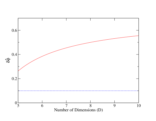
Figure 1: The fractional difference ($\delta\hat{\varphi}$) of the GW phase with respect to that of the $4d$ GR as a function of the number of dimensions ($D$). The blue dashed line shows the upper bound placed on $\delta\hat{\varphi}$ from the combined events of the first and second observing runs of the LIGO/Virgo Abbott et al. (2019b).

We now comment on some caveat in the above bounds. We used the bounds derived by the LIGO/Virgo Collaborations that assumed the correction to 4d GR in the phase enters only at 0PN order. Such a correction partially degenerates with the chirp mass that also enters first at 0PN order, though the mass also enters at higher PN orders and thus the degeneracy can be partially broken. In reality, higher PN corrections to 4d GR also enter in the waveform phase. This may change the amount of correlation between the chirp mass and beyond-4d-GR effects and may weaken the bound on the 0PN correction. In Abbott et al. (2016a), the LIGO/Virgo Collaborations carried out another analysis for GW150914 where they included phase corrections at various PN orders in the search parameter set. This enhances the correlation significantly and the bound on the 0PN correction now becomes $|\delta\hat{\varphi}|\lesssim 5$. If we quote this bound, we cannot rule out the compact extra dimension model considered here. Thus, to make a robust statement on whether one can rule out the model with gravitational-wave observations, one needs to compute corrections at higher PN orders and rederive bounds on the extra dimension effect.

Having said this, one can still rule out the model with binary pulsar observations for the following reason. A standard method for testing GR with binary pulsars is to determine the masses from at least three independent observables (such as post-Keplerian parameters including the periastron precession, Shapiro delay and orbital decay rate) assuming GR and check the consistency. The orbital decay rate $\dot{P}$ is the only post-Keplerian parameter that depends on the gravitational-wave emission. Thus, even for the compact extra dimension model considered here, one can safely use the masses obtained from other post-Keplerian parameters under the 4d GR assumption since the conservative corrections are exponentially suppressed. One can then use the measurement of $\dot{P}$ to constrain the model without having to worry about the degeneracy between the extra dimension effect and masses. Such $\dot{P}$ measurements have been mapped to a bound on $\delta\hat{\varphi}$ as $|\delta\hat{\varphi}|\lesssim 10^{-3}$ Yunes and Hughes (2010); Nair and Yunes (2020), which is much stronger than the gravitational-wave bound. Thus, one can rule out the compact dimension model with the binary pulsar observations.

VIII Conclusions

In this paper we performed an analysis of gravitational waves sourced by a binary in a $D$-dimensional spacetime with four non-compact dimensions and a set of compactified extra dimensions. We worked under the assumptions that the two binary sources are point-like and located on the same ”brane” (i.e. at the same position in the compact coordinates). For most part we took $D=5$, but we have provided generalizations to arbitrary $D$ throughout the paper. We worked within the framework of GR, and in the limit of small extra dimensions. We computed the gravitational waves sourced by the binary, the luminosity of the gravitational waves and the phase of the gravitational waves, to leading order in the post-Newtonian expansion. We found that the luminosity of gravitational waves emitted in $5d$ gravity by a binary with the same characteristics (same masses and separation distance) as a $4d$ binary is 20.8% less relative to the $4d$ case, to leading post-Newtonian order. The phase of the gravitational waveform differs by 26% relative to the $4d$ case, to leading post-Newtonian order, while for general $D$, the fractional difference of the phase with that of $4d$ GR is $\frac{5(D-4)}{7D-16}$, which only increases with an increase in $D$. While there are exponential corrections which depend on the size of the extra dimensions, the leading order estimates for the gravitational wave phase we gave here are independent of size, and depend only on the number of extra dimensions. Based on a comparison with gravitational-wave observations from the LIGO/Virgo Collaborations Abbott et al. (2019b) and binary pulsar observations from radio astronomy Yunes and Hughes (2010); Nair and Yunes (2020) we can rule out this class of models for compact extra dimensions. The main source of discrepancy is the higher-dimensional gravity coupling with matter, which, when seen from a $4d$ perspective, means that matter will couple not only with the $4d$ metric, but with the dilaton as well. This dilaton coupling (or scalar charge) is responsible for fifth force effects which change the phase of the gravitational waves. Our results agree with those derived in the context of $4d$ Einstein-Maxwell-dilaton theory Julié (2018a, b); Khalil et al. (2018) provided that we set the binary’s scalar charges equal to one another and equal to the Kaluza-Klein value.

The same fifth force effects are responsible for the difference between the $4d$ Newton’s constant $G_{\rm N}$ and the $4d$ gravitational coupling $G$: $G_{N}=\frac{2(D-3)}{D-2}G$, and for the Shapiro time-delay discrepancy with $4d$ GR. In a parametrized post-Newtonian expansion (PPN) the $4d$ “physical” metric (which is obtained by performing a rescaling of the $4d$ metric with the dilaton in such a way to eliminate the matter-dilaton coupling Will (2006) is written as $g_{00}=-1+2U+\dots,g_{ij}=\delta_{ij}(1+2\gamma\,U+\dots)$, with $\gamma=1$ in $4d$ GR. A measurement of the frequency shift of radio photons to and from the Cassini spacecraft as they passed near the Sun gave $\gamma=1+(2.1\pm 2.3)\times 10^{-5}$ Bertotti et al. (2003). On the other hand, the “physical metric” as read off from footnote 1 has $g_{00}=-1+\frac{2}{3}\tilde{h}_{\rm T}{}_{00}$ and $g_{ij}=1+\frac{1}{3}\tilde{h}_{\rm T}{}_{00}+\dots$, which amounts to $\gamma\sim 1/2$. Therefore this class of compactified extra dimensions models was ruled out based on Solar System measurements Xu and Ma (2007); Deng and Xie (2015).

In string theory the massless dilaton is one of the many moduli (zero mass scalars) that arise in the compactification of the higher-dimensional spacetime. Stabilzation of the moduli can be achieved, for example, by turning on fluxes for the Ramond-Ramond potentials Kachru et al. (2003). This gives rise to a mass term for the moduli, and eliminates the large contribution of the scalar fifth force, by turning a Coulomb potential into a Yukawa potential. It would be interesting to study gravitational waves in such a set-up and place constraints on the various parameters. A somewhat simpler scenario is the Randall-Sundrum model, where the fifth dimension is large and warped. Our work here is intended as a first step in understanding how to set up the problem of solving for gravitational waves in a higher-dimensional space with compact dimensions, or warped, large extra dimensions. For example, we saw that quadrupole formula need not apply, and we had to use a direct integration of the Einstein equations. Also, when it comes to the propagation of gravitational waves in spacetimes with warped, large extra dimensions, reducing the problem to $4d$ seems less appropriate, and working in the higher-dimensional space, as we did here, presents an advantage.

Appendix A Modified quadrupole formula

Here we explicitly point out why the usual quadrupole formula

$$\int d^{3}\vec{x}\,\tau^{ij}=\frac{1}{2}\partial_{0}^{2}\int d^{3}\vec{x}\,\tau^{00}x^{i}x^{j}\,,$$ (93)

cannot be directly extended to higher dimensions if there are compact dimensions.

Consider the expression $\frac{1}{2}\partial_{0}^{2}\int d^{3}\vec{x}\int_{0}^{l}dw\,\tau^{00}x^{I}x^{J}$, then use repeatedly the conservation law for $\tau^{MN}$ and integrate by parts, while paying attention to the boundary terms:

$$\frac{1}{2}\partial_{0}^{2}\int d^{3}\vec{x}\int_{0}^{l}dw\,\tau^{00}x^{I}x^{J}=\int d^{3}\vec{x}\int_{0}^{l}dw\,\tau^{IJ}+\frac{1}{2}\int d^{3}\vec{x}(\partial_{K}\tau^{5K}x^{I}x^{J}-\tau^{5I}x^{J}-\tau^{5J}x^{I})\Big{|}_{w=0}^{w=l}\,.$$

For $I,J=i,j=1,2,3$, the quadrupole formula applies because of the periodicity of the metric fluctuations in $w$. However if either $I$ or $J$ are along the compact dimension, then there are extra terms relative to those expected based on the quadrupole formula. These terms are not straightforward to evaluate, and for this reason we rely on direct integration of the Einstein equations.

Appendix B Hidden Brane Scenario

We generalize the Newtonian potential by having the observer located at $w=0$, and the static mass source $m$ on a hidden brane at $w=w_{1}$:

$$T_{00}(x^{\mu},w)=m\delta^{3}(\vec{x})\delta(w-w_{1})\,.$$ (95)

The corresponding Newtonian potential evaluated by the observer is

$$V^{(5,c)}(R,w_{1})=-\frac{4}{3\pi}G^{(5)}m\sum_{n=-\infty}^{\infty}\frac{1}{R^{2}+\left(w_{1}+nl\right)^{2}}\,.$$ (96)

Using Poisson summation, the above sum can be evaluated to give the following result:

$$V^{(5,c)}(R,w_{1})= -\frac{4}{3}\frac{G^{(5)}m}{lR}\tanh{\frac{2\pi R}{l}}\left(1+\operatorname{sech}\frac{2\pi R}{l}\cos\frac{2\pi w_{1}}{l}\right)$$

$$\simeq-\frac{4}{3}\frac{G^{(5)}m}{lR}\left(1+2e^{-2\pi R/l}\cos\frac{2\pi w_{1}}{l}\right)\,,$$ (97)

where in the last step we used $R\gg l$ and $R\gg w_{1}$. When $w_{1}=0$, (B) reproduces the Newtonian potential in Section III in the limit of $2\pi R\gg l$.

Appendix C Newtonian Potential from integrating the retarded $5d$ compactified Green’s function

In this appendix we offer an alternative derivation of the Newtonian potential obtained in Section III, by using the retarded $5d$ compactified Green’s function. A static source of mass $m$ located at the origin has

$$T_{00}(x^{\mu},w)=m\delta^{3}(\vec{x})\delta(w)\,.$$ (98)

Substituting  (43) and (98) into  (40) we obtain

$$\tilde{h}_{\rm T,00}\left(x^{\mu},w\right) =-\frac{4}{\pi}G^{(5)}m\sum_{n=-\infty}^{\infty}\frac{1}{r_{n}}\int_{0}^{\infty}dt^{\prime}\,\frac{\partial}{\partial r_{n}}\frac{\theta\left(t-t^{\prime}-r_{n}\right)}{\sqrt{\left(t-t^{\prime}\right)^{2}-r_{n}^{2}}}\,,$$ (99)

where $r_{n}=\sqrt{x^{2}+y^{2}+z^{2}+(w-nl)^{2}}$. The integral in (99) can be evaluated by re-expressing the $\partial_{r_{n}}$ derivative in terms of a time-derivative using

$$\frac{\partial}{\partial r_{n}}\left[\frac{\theta\left(\Delta t-r_{n}\right)}{\left(\Delta t^{2}-r_{n}^{2}\right)^{1/2}}\right]= -\frac{\partial}{\partial\Delta t}\left[\frac{\theta\left(\Delta t-r_{n}\right)}{\left(\Delta t^{2}-r_{n}^{2}\right)^{1/2}}\right]+\frac{\theta\left(\Delta t-r_{n}\right)}{\left[(\Delta t)^{2}-r_{n}^{2}\right]^{3/2}}\left(r_{n}-\Delta t\right)\,,$$ (100)

where $\Delta t=t-t^{\prime}$. Substituting (100) into (99) we obtain

$$\tilde{h}_{\rm T}^{00}(x^{\mu},w)= -\frac{4}{\pi}G^{(5)}m\sum_{n=-\infty}^{\infty}\frac{1}{r_{n}}\int_{r_{n}}^{\infty}d\Delta t\frac{r_{n}-\Delta t}{\left[(\Delta t)^{2}-r_{n}^{2}\right]^{3/2}}=\frac{4}{\pi}G^{(5)}m\sum_{n=-\infty}^{\infty}\frac{1}{r_{n}^{2}}\,,$$ (101)

and the corresponding Newton’s potential $V^{(5,c)}\equiv(-1/3)\tilde{h}_{\rm T,00}$ matches with the one in Eq. (17).

Appendix D Retarded Green’s function

The massless scalar $D$-dimensional flat space Euclidean Green’s function $\mathcal{G}_{\rm E}(x,x^{\prime})=\mathcal{G}_{\rm E}(x-x^{\prime})$ is the inverse of the $D$-dimensional Laplacian

$$\Delta_{(D)}\mathcal{G}^{(D)}E(x-x^{\prime})=\delta^{D}(x-x^{\prime}),\qquad\mathcal{G}^{(D)}_{\rm E}(x-x^{\prime})=-\int\frac{d^{D}p}{(2\pi)^{D}}\frac{e^{ip\cdot x}}{p\cdot p}.$$ (102)

Starting from the unique Euclidean Green’s function, in Minkowski signature the retarded Green’s function is obtained via the analytical continuation $p^{0}_{\rm E}\longrightarrow-i(p^{0}+i\epsilon)$. The Euclidean metric $\delta^{MN}$ gets replaced by the Minkowski metric $\eta^{MN}$, and the $i\epsilon$ prescription yields the retarded Green’s function:

$$\mathcal{G}^{(D)}(x-x^{\prime})=-\int\frac{d^{D}p}{(2\pi)^{D}}\,\frac{e^{ip\cdot x}}{-(p^{0}+i\epsilon)^{2}+p^{i}p^{i}}.$$ (103)

The location of the poles is in the lower half-plane, when viewed as a function of $p^{0}$ as a complex variable. To evaluate the integral one integrates over $p^{0}$, using Cauchy’s theorem, and if $t-t^{\prime}>0$, one picks up the contribution from the two poles, otherwise the retarded Green’s function is zero. If $D=4$, we recover the familiar expression

$$\mathcal{G}^{(4)}(x-x^{\prime})=-\theta(t-t^{\prime})\int\frac{d^{3}p}{(2\pi)^{3}}\frac{\sin(p(t-t^{\prime}))}{p}e^{i\vec{p}\cdot(\vec{x}-\vec{x}^{\prime})}=-\theta(t-t^{\prime})\frac{1}{4\pi r}\delta((t-t^{\prime})-|\vec{x}-\vec{x}^{\prime}|),$$ (104)

where we used $p$ to denote the magnitude of the spatial vector $\vec{p}$, i.e. $p=|\vec{p}|$. If $D=5$, then

$$\mathcal{G}^{(5)}(x-x^{\prime}) =-\theta(t-t^{\prime})\int\frac{d^{4}p}{(2\pi)^{4}}\frac{\sin(p(t-t^{\prime}))}{p}e^{i\vec{p}\cdot(\vec{x}-\vec{x}^{\prime})}$$

$$=-\theta(t-t^{\prime})\frac{4\pi}{(2\pi)^{4}}\int_{0}^{\infty}dp\,p^{3}\int_{0}^{\pi}d\theta\,\sin^{2}\theta\,\frac{\sin(p(t-t^{\prime}))}{p}e^{ip|\vec{x}-\vec{x}^{\prime}|\cos\theta}$$

$$=-\theta(t-t^{\prime})\frac{1}{4\pi^{2}|\vec{x}-\vec{x}^{\prime}|}\int_{0}^{\infty}dp\,p\sin(p(t-t^{\prime}))J_{1}(p|\vec{x}-\vec{x}^{\prime}|)$$

$$=-\theta(t-t^{\prime})\frac{1}{4\pi^{2}|\vec{x}-\vec{x}^{\prime}|}\frac{\partial}{\partial|\vec{x}-\vec{x}^{\prime}|}\int_{0}^{\infty}dp\,\sin(p(t-t^{\prime}))J_{0}(p|\vec{x}-\vec{x}^{\prime}|)$$

$$=-\theta(t-t^{\prime})\frac{1}{4\pi^{2}|\vec{x}-\vec{x}^{\prime}|}\frac{\partial}{\partial|\vec{x}-\vec{x}^{\prime}|}\frac{\theta(t-t^{\prime}-|\vec{x}-\vec{x}^{\prime}|)}{\sqrt{(t-t^{\prime})^{2}-(\vec{x}-\vec{x}^{\prime})^{2}}}\,.$$ (105)

Appendix E Direct Integration vs. Quadrupole Formula

Here we use post-Newtonian order counting to explain a somewhat subtle aspect of our calculations. For simplicity’s sake, in this appendix we restrict ourselves to $4d$ GR. Specifically, we will show that if in computing the spatial metric fluctuations $\tilde{h}^{ij}$, one uses the quadrupole formula, then one can safely neglect nonlinear source terms in the relaxed Einstein equations. However, if one directly integrates the relaxed Einstein equations, then the nonlinear terms cannot be neglected already at the leading post-Newtonian order. Since our goal is only to highlight the dependence on velocities, we will write our equations with squiggle lines, signaling that we are imprecise about numerical factors.

The relaxed Einstein equations in the harmonic gauge are given in (8), whose $4d$ solution is given by

$$\tilde{h}^{\mu\nu}\sim\frac{4}{R}\int d^{3}\vec{x}\,\tau^{\mu\nu}(\vec{x},t-R)\,,$$ (106)

where we assumed that we are working in the far-field approximation, $R$ is the distance from the source to the field point, and the right hand side is evaluated at the retarded time.

E.1 Direct Integration

We are interested in extracting the order of magnitude in a post-Newtonian (PN) expansion estimates of the spatial components $\tilde{h}^{ij}$ for a compact binary. We will be somewhat careless about the indices and numerical factors since we only care about counting the PN order, namely powers of the relative velocity of the binary constituents, $v$. Eq. (106) should receive contributions from both $T^{ij}$ and $t_{\rm{LL}}^{ij}$. To leading PN order, the contribution from $T^{ij}$ is roughly given by

$$\tilde{h}^{ij}_{\rm T}\sim\frac{\mu}{R}v^{i}v^{j}\sim\frac{\mu}{R}v^{2}\,,$$ (107)

where $\mu$ is the reduced mass of the binary. To consider the contribution of $t_{\rm{LL}}^{ij}$, let us substitute $\tilde{g}^{ij}=\eta^{ij}-\tilde{h}^{ij}$ into (II) and look at one term (inside $t_{\rm{LL}}^{ij}$), for example

$$(-g)t_{\rm{LL}}^{ij}\sim\tilde{h}^{00}{}^{,i}\tilde{h}_{00}{}^{,j}\sim\tilde{h}_{00}{}_{,i}\tilde{h}_{00}{}_{,j}\,,$$ (108)

so that

$$\tilde{h}^{ij}_{\rm{t}}\sim\frac{1}{R}\int d^{3}x\,\tilde{h}_{00}{}_{,i}\tilde{h}_{00}{}_{,j}\,.$$ (109)

To compute (109), let us consider partitioning the spacetime into a near zone (NZ) and a far zone (FZ) relative to the location of the sources. NZ is the region centered around the source with the size of the gravitational wavelength while FZ is the region exterior to it Pati and Will (2000). Within the NZ, the gravitational fields can be considered as almost instantaneous and retardation can be neglected. The integral in (109) can be decomposed into the NZ and FZ integrals. It turns out that the former dominates the latter, so what we need is the NZ solution for $\tilde{h}_{00}$. For a compact binary, the leading NZ solution is given by Blanchet et al. (1998)

$$h_{00}^{\mathrm{NZ}} \sim \frac{2m_{1}}{r_{1}}+\frac{2m_{2}}{r_{2}}\,,$$ (110)

$$h_{ij}^{\mathrm{NZ}} \sim \left(\frac{2m_{1}}{r_{1}}+\frac{2m_{2}}{r_{2}}\right)\delta_{ij}\,,$$ (111)

with $r_{a}\equiv|\vec{x}-\vec{x}_{a}|$ and where $a=1,2$ corresponding to one of the two sources. Thus, $h^{\mathrm{NZ}}\sim 4m_{1}/r_{1}+4m_{2}/r_{2}$ and

$$\tilde{h}_{00}^{\mathrm{NZ}}\sim h_{00}^{\mathrm{NZ}}-\frac{1}{2}h^{\mathrm{NZ}}\eta_{00}\sim\frac{4m_{1}}{r_{1}}+\frac{4m_{2}}{r_{2}}\,.$$ (112)

We now substitute the above equation into the right hand side of (109). Those terms that only depend on $r_{1}$ or $r_{2}$ will diverge and be dropped upon regularization, so what matters is the cross term between sources 1 and 2. Ignoring numerical factors, we find

$$\tilde{h}^{ij}_{\rm{t}} \sim \frac{m_{1}m_{2}}{R}\int_{\mathrm{NZ}}d^{3}x\,\partial_{i}\left(\frac{1}{r_{1}}\right)\partial_{j}\left(\frac{1}{r_{2}}\right)+(1\leftrightarrow 2)$$ (113)

$$\sim \frac{m_{1}m_{2}}{R}\int_{\mathrm{NZ}}d^{3}x\,\partial_{i}^{(1)}\left(\frac{1}{r_{1}}\right)\partial_{j}^{(2)}\left(\frac{1}{r_{2}}\right)+(1\leftrightarrow 2)$$

$$\sim \frac{m_{1}m_{2}}{R}\partial_{i}^{(1)}\partial_{j}^{(2)}\int_{\mathrm{NZ}}d^{3}x\,\frac{1}{r_{1}r_{2}}+(1\leftrightarrow 2)\,,$$

where we changed the partial derivatives to source-derivatives $\partial_{i}^{(a)}\equiv\partial/\partial x^{i}_{a}$ so that derivatives can be taken outside of the integral. The remaining integral, is given by Blanchet et al. (2002)

$$\int_{\mathrm{NZ}}d^{3}x\,\frac{1}{r_{1}r_{2}}=-2\pi r_{12}\,,$$ (114)

where $r_{12}=|\vec{x}_{1}-\vec{x}_{2}|$ is the binary separation. Thus,

$$\tilde{h}^{ij}_{\rm{t}} \sim \frac{m_{1}m_{2}}{R}\partial_{i}^{(1)}\partial_{j}^{(2)}r_{12}+(1\leftrightarrow 2)$$ (115)

$$\sim \frac{m_{1}m_{2}}{R}\frac{1}{r_{12}}$$

$$\sim \frac{\mu}{R}\frac{M}{r_{12}}$$

$$\sim \frac{\mu}{R}v^{2}\,,$$

where $M$ is the total mass and we used the Kepler’s law in the last equation. This scaling could in fact be easily obtained from the first line of (113) by replacing all the length scales inside the integral with $r_{12}$. Notice that $\tilde{h}^{ij}_{\rm{t}}$ is of the same PN order as $\tilde{h}^{ij}_{\rm T}$. This means that the contribution from $t_{\rm{LL}}^{ij}$ cannot be neglected even at the leading order.

E.2 Quadrupole Formula

So far we have seen that by using direct integration of the relaxed Einstein equations, where $\tilde{h}^{ij}$ is sourced by $\tau^{ij}$, both the linearized $\tilde{h}^{ij}_{\rm T}$ and second order in fluctuation $\tilde{h}^{ij}_{\rm{t}}$ are of the same order in a velocity expansion. However, if we replace our starting point for the derivation of $\tilde{h}^{ij}$ with the quadrupole formula (see Appendix A)

$$\int\tau^{ij}d^{3}x=\frac{1}{2}\frac{d^{2}}{dt^{2}}\int d^{3}x\,\tau^{00}x^{i}x^{j}\,,$$ (116)

then we would be using $\tau^{00}$ in extracting $\tilde{h}^{ij}$. In this case, the contribution from $t_{\rm{LL}}^{00}$ is subleading to that of $T^{00}$, as we will now show.

Using (116) and (106) one derives

$$\tilde{h}^{ij}\sim\frac{2}{R}\frac{d^{2}}{dt^{2}}\int d^{3}x\,\tau^{00}x^{i}x^{j}\,.$$ (117)

The contribution from $T^{00}$ has the same scaling as in (107), i.e.

$$\tilde{h}^{ij}_{(T^{00})}\sim\frac{\mu}{R}v^{2}\,.$$ (118)

On the other hand, the contribution from $t^{00}$ is given by

$$\tilde{h}^{ij}_{(t^{00})} \sim \frac{1}{R}\frac{d^{2}}{dt^{2}}\int_{\mathrm{NZ}}d^{3}x\,\tilde{h}_{00}^{\mathrm{NZ}}{}_{,i}\tilde{h}_{00}^{\mathrm{NZ}}{}_{,j}\,x^{i}x^{j}$$ (119)

$$\sim \frac{1}{R}\frac{d^{2}}{dt^{2}}\int_{\mathrm{NZ}}d^{3}x\,\partial_{i}\left(\frac{m_{1}}{r_{1}}\right)\partial_{j}\left(\frac{m_{2}}{r_{2}}\right)\,x^{i}x^{j}$$

$$\sim \frac{1}{R}\Omega^{2}\frac{m_{1}}{r_{12}^{2}}\frac{m_{2}}{r_{12}^{2}}r_{12}^{2}r_{12}^{3}$$

$$\sim \frac{m_{1}m_{2}}{R}r_{12}\Omega^{2}$$

$$\sim \frac{\mu}{R}\frac{M}{r_{12}}(r_{12}\Omega)^{2}$$

$$\sim \frac{\mu}{R}v^{4}\,,$$

where $\Omega$ is the binary angular frequency and we replaced all the length scale by $r_{12}$ in the third line as noted in Sec. E.1. Notice that $\tilde{h}^{ij}_{(\rm{t}^{00})}$ is of higher order in velocities than $\tilde{h}^{ij}_{(\rm T^{00})}$. Thus, once the expression for $\tilde{h}^{ij}$ is turned into the quadrupole formula, the contribution from $t^{00}$ becomes subdominant and one only needs to consider $T^{00}$ to leading order.

Appendix F GW luminosity in Transverse-Traceless (TT) Gauge

The transverse traceless (TT) gauge for linearized gravitational fluctuations about a flat spacetime imposes the following conditions:

$$\tilde{h}^{{\mbox{\tiny TT}}}_{0M}=0\,,\qquad(\tilde{h}^{{\mbox{\tiny TT}}})\indices{{}^{I}_{I}}=0\,,\qquad\partial_{J}(\tilde{h}^{{\mbox{\tiny TT}}})^{IJ}=0\,.$$ (120)

Starting from the trace-reversed metric fluctuations, $\tilde{h}_{IJ}$, one can show that the transverse traceless components are obtained by simply acting with a transverse-tracelss projector

$$\Lambda_{IJKL}=P_{IK}P_{JL}-\frac{1}{D-2}P_{IJ}P_{KL}\,,$$ (121)

and where $P_{IK}$ are projectors orthogonal to $n^{I}$, with $n^{I}$ the direction of propagation of the waves and $n^{I}n^{I}=1$:

$$P_{IJ}=\delta_{IJ}-n_{I}n_{J}\,,\qquad P_{IJ}n^{J}=0\,.$$ (122)

Therefore, the non-vanishing (same as the trace-reversed) metric fluctuations in the TT gauge are

$$\tilde{h}_{IJ}^{{\mbox{\tiny TT}}}=\Lambda_{IJKL}\tilde{h}^{KL}\,,\qquad(\tilde{h}^{{\mbox{\tiny TT}}})^{I}{}_{I}=0\,,\qquad n^{I}\tilde{h}_{IJ}^{{\mbox{\tiny TT}}}=\tilde{h}_{IJ}^{{\mbox{\tiny TT}}}n^{J}=0\,.$$ (123)

It is easy to verify that

$$\tilde{h}^{{\mbox{\tiny TT}}}_{IJ}(\tilde{h}^{{\mbox{\tiny TT}}})^{IJ}= \tilde{h}_{IJ}\tilde{h}^{IJ}-2n^{I}n^{J}\delta^{KL}\tilde{h}_{IK}\tilde{h}_{JL}+\left(\dfrac{D-3}{D-2}\right)n^{I}n^{J}n^{K}n^{L}\tilde{h}_{IJ}\tilde{h}_{KL}$$ (124)

$$-\left(\dfrac{1}{D-2}\right)(\tilde{h}^{I}{}_{I})^{2}+\left(\dfrac{2}{D-2}\right)n^{K}n^{L}\tilde{h}_{KL}\tilde{h}^{I}{}_{I}\,.$$

In particular, working in the TT gauge, the equation (66) becomes simply

$$t_{0K}n^{K}=-\frac{1}{32\pi G^{(D)}}\left\langle\dot{\tilde{h}}^{{\mbox{\tiny TT}}}_{IJ}(\dot{\tilde{h}}^{{\mbox{\tiny TT}}})^{IJ}\right\rangle\,.$$ (125)

We can nevertheless recover (71), starting from the TT gauge expression (125) and substituting (124), which is to be expected given that we are computing a gauge-invariant quantity.

References

• Abbott et al. (2016a) B. P. Abbott et al. (LIGO Scientific, Virgo), Phys. Rev. Lett. 116, 221101 (2016a), [Erratum: Phys. Rev. Lett.121,no.12,129902(2018)], eprint 1602.03841.
• Yunes et al. (2016) N. Yunes, K. Yagi, and F. Pretorius, Phys. Rev. D94, 084002 (2016), eprint 1603.08955.
• Abbott et al. (2016b) B. P. Abbott et al. (LIGO Scientific, Virgo), Phys. Rev. X6, 041015 (2016b), [erratum: Phys. Rev.X8,no.3,039903(2018)], eprint 1606.04856.
• Abbott et al. (2019a) B. P. Abbott et al. (LIGO Scientific, Virgo), Phys. Rev. Lett. 123, 011102 (2019a), eprint 1811.00364.
• Abbott et al. (2019b) B. P. Abbott et al. (LIGO Scientific, Virgo), Phys. Rev. D100, 104036 (2019b), eprint 1903.04467.
• Berti et al. (2018a) E. Berti, K. Yagi, and N. Yunes, Gen. Rel. Grav. 50, 46 (2018a), eprint 1801.03208.
• Berti et al. (2018b) E. Berti, K. Yagi, H. Yang, and N. Yunes, Gen. Rel. Grav. 50, 49 (2018b), eprint 1801.03587.
• Will (1993) C. M. Will, Theory and Experiment in Gravitational Physics (Cambridge University Press, 1993).
• Will (2006) C. M. Will, Living Reviews in Relativity 9 (2006), eprint gr-qc/0510072, URL http://www.livingreviews.org/lrr-2006-3.
• Stairs (2003) I. H. Stairs, Living Rev.Rel. 6, 5 (2003), eprint astro-ph/0307536.
• Wex (2014) N. Wex (2014), eprint 1402.5594.
• Jain and Khoury (2010) B. Jain and J. Khoury, Annals Phys. 325, 1479 (2010), eprint 1004.3294.
• Koyama (2016) K. Koyama, Rept. Prog. Phys. 79, 046902 (2016), eprint 1504.04623.
• Cardoso et al. (2003) V. Cardoso, O. J. C. Dias, and J. P. S. Lemos, Phys. Rev. D67, 064026 (2003), eprint hep-th/0212168.
• Pardo et al. (2018) K. Pardo, M. Fishbach, D. E. Holz, and D. N. Spergel, JCAP 1807, 048 (2018), eprint 1801.08160.
• Kol and Smolkin (2012) B. Kol and M. Smolkin, JHEP 02, 010 (2012), eprint 1110.3764.
• Cardoso et al. (2019) V. Cardoso, L. Gualtieri, and C. J. Moore, Phys. Rev. D100, 124037 (2019), eprint 1910.09557.
• Hirschmann et al. (2018) E. W. Hirschmann, L. Lehner, S. L. Liebling, and C. Palenzuela, Phys. Rev. D97, 064032 (2018), eprint 1706.09875.
• Julié (2018a) F.-L. Julié, JCAP 1801, 026 (2018a), eprint 1711.10769.
• Julié (2018b) F.-L. Julié, JCAP 1810, 033 (2018b), eprint 1809.05041.
• Khalil et al. (2018) M. Khalil, N. Sennett, J. Steinhoff, J. Vines, and A. Buonanno, Phys. Rev. D98, 104010 (2018), eprint 1809.03109.
• Andriot and Lucena Gómez (2017) D. Andriot and G. Lucena Gómez, JCAP 1706, 048 (2017), [Erratum: JCAP1905,no.05,E01(2019)], eprint 1704.07392.
• Andriot and Tsimpis (2019) D. Andriot and D. Tsimpis (2019), eprint 1911.01444.
• Kwon et al. (2019) O.-K. Kwon, S. Lee, and D. D. Tolla, Phys. Rev. D100, 084050 (2019), eprint 1906.11652.
• Toshmatov et al. (2016) B. Toshmatov, Z. Stuchlík, J. Schee, and B. Ahmedov, Phys. Rev. D93, 124017 (2016), eprint 1605.02058.
• Chakraborty et al. (2018) S. Chakraborty, K. Chakravarti, S. Bose, and S. SenGupta, Phys. Rev. D97, 104053 (2018), eprint 1710.05188.
• Chakravarti et al. (2019a) K. Chakravarti, S. Chakraborty, S. Bose, and S. SenGupta, Phys. Rev. D99, 024036 (2019a), eprint 1811.11364.
• Chakravarti et al. (2019b) K. Chakravarti, S. Chakraborty, K. S. Phukon, S. Bose, and S. SenGupta (2019b), eprint 1903.10159.
• Randall and Sundrum (1999) L. Randall and R. Sundrum, Phys. Rev. Lett. 83, 4690 (1999), eprint hep-th/9906064.
• Emparan et al. (2002) R. Emparan, A. Fabbri, and N. Kaloper, JHEP 08, 043 (2002), eprint hep-th/0206155.
• Tanaka (2003) T. Tanaka, Prog. Theor. Phys. Suppl. 148, 307 (2003), eprint gr-qc/0203082.
• Adelberger et al. (2007) E. G. Adelberger, B. R. Heckel, S. A. Hoedl, C. D. Hoyle, D. J. Kapner, and A. Upadhye, Phys. Rev. Lett. 98, 131104 (2007), eprint hep-ph/0611223.
• Kapner et al. (2007) D. J. Kapner, T. S. Cook, E. G. Adelberger, J. H. Gundlach, B. R. Heckel, C. D. Hoyle, and H. E. Swanson, Phys. Rev. Lett. 98, 021101 (2007), eprint hep-ph/0611184.
• Caldwell and Langlois (2001) R. R. Caldwell and D. Langlois, Phys. Lett. B511, 129 (2001), eprint gr-qc/0103070.
• Abdalla et al. (2002a) E. Abdalla, B. Cuadros-Melgar, S.-S. Feng, and B. Wang, Phys. Rev. D65, 083512 (2002a), eprint hep-th/0109024.
• Abdalla et al. (2002b) E. Abdalla, A. Casali, and B. Cuadros-Melgar, Nucl. Phys. B644, 201 (2002b), eprint hep-th/0205203.
• Abdalla and Cuadros-Melgar (2003) E. Abdalla and B. Cuadros-Melgar, Phys. Rev. D67, 084012 (2003), eprint hep-th/0209101.
• Abdalla et al. (2004) E. Abdalla, A. G. Casali, and B. Cuadros-Melgar, Int. J. Theor. Phys. 43, 801 (2004), eprint hep-th/0501076.
• Yu et al. (2017) H. Yu, B.-M. Gu, F. P. Huang, Y.-Q. Wang, X.-H. Meng, and Y.-X. Liu, JCAP 1702, 039 (2017), eprint 1607.03388.
• Visinelli et al. (2018) L. Visinelli, N. Bolis, and S. Vagnozzi, Phys. Rev. D97, 064039 (2018), eprint 1711.06628.
• Yu et al. (2019) H. Yu, Z.-C. Lin, and Y.-X. Liu, Commun. Theor. Phys. 71, 991 (2019), eprint 1905.10614.
• Lin et al. (2020) Z.-C. Lin, H. Yu, and Y.-X. Liu, Physical Review D 101 (2020), ISSN 2470-0029, URL http://dx.doi.org/10.1103/PhysRevD.101.104058.
• Pati and Will (2000) M. E. Pati and C. M. Will, Phys. Rev. D62, 124015 (2000), eprint gr-qc/0007087.
• Landau and Lifschits (1975) L. Landau and E. Lifschits, The Classical Theory of Fields, vol. Volume 2 of Course of Theoretical Physics (Pergamon Press, Oxford, 1975), ISBN 978-0-08-018176-9.
• Yoshino and Shibata (2009) H. Yoshino and M. Shibata, Phys. Rev. D80, 084025 (2009), eprint 0907.2760.
• Zwiebach (2006) B. Zwiebach, A first course in string theory (Cambridge University Press, 2006), ISBN 0521831431, 9780521831437, 9780511207570, URL http://www.cambridge.org/uk/catalogue/catalogue.asp?isbn=0521831431.
• Fichet (2020) S. Fichet, Braneworld effective field theories–holography, consistency and conformal effects (2020), eprint 1912.12316.
• Duff et al. (1986) M. J. Duff, B. E. W. Nilsson, and C. N. Pope, Phys. Rept. 130, 1 (1986).
• Dai and Stojkovic (2013) D.-C. Dai and D. Stojkovic, Eur. Phys. J. Plus 128, 122 (2013), eprint 1309.2996.
• Brill and Hartle (1964) D. R. Brill and J. B. Hartle, Phys. Rev. 135, B271 (1964).
• Damour and Esposito-Farese (1992) T. Damour and G. Esposito-Farese, Class. Quant. Grav. 9, 2093 (1992).
• Maggiore (2007) M. Maggiore, Gravitational Waves. Vol. 1: Theory and Experiments, Oxford Master Series in Physics (Oxford University Press, 2007), ISBN 978-0-19-857074-5, 978-0-19-852074-0.
• Cutler and Flanagan (1994) C. Cutler and E. E. Flanagan, Phys. Rev. D49, 2658 (1994), eprint gr-qc/9402014.
• Yunes and Hughes (2010) N. Yunes and S. A. Hughes, Phys. Rev. D82, 082002 (2010), eprint 1007.1995.
• Nair and Yunes (2020) R. Nair and N. Yunes (2020), eprint 2002.02030.
• Durrer and Kocian (2004) R. Durrer and P. Kocian, Class. Quant. Grav. 21, 2127 (2004), eprint hep-th/0305181.
• Bertotti et al. (2003) B. Bertotti, L. Iess, and P. Tortora, Nature 425, 374 (2003).
• Xu and Ma (2007) P. Xu and Y.-g. Ma, Phys. Lett. B656, 165 (2007), eprint 0710.3677.
• Deng and Xie (2015) X.-M. Deng and Y. Xie, Eur. Phys. J. C75, 539 (2015), eprint 1510.02946.
• Kachru et al. (2003) S. Kachru, R. Kallosh, A. D. Linde, and S. P. Trivedi, Phys. Rev. D68, 046005 (2003), eprint hep-th/0301240.
• Blanchet et al. (1998) L. Blanchet, G. Faye, and B. Ponsot, Phys. Rev. D58, 124002 (1998), eprint gr-qc/9804079.
• Blanchet et al. (2002) L. Blanchet, B. R. Iyer, and B. Joguet, Phys. Rev. D65, 064005 (2002), [Erratum: Phys. Rev.D71,129903(2005)], eprint gr-qc/0105098.