Deciphering the large-scale environment of radio galaxies in the local Universe II.
A statistical analysis of environmental properties
Abstract
In our previous analysis we investigated the large-scale environment of two samples of radio galaxies (RGs) in the local Universe (i.e. with redshifts 0.15), classified as FR I and FR II on the basis of their radio morphology. The analysis was carried out using i) extremely homogeneous catalogs and ii) a new method, known as cosmological overdensity, to investigate their large-scale environments. We concluded that, independently by the shape of their radio extended structure, RGs inhabit galaxy-rich large-scale environments with similar characteristics and richness. In the present work, we first highlight additional advantages of our procedure, that does not suffer cosmological biases and/or artifacts, and then we carry out an additional statistical test to strengthen our previous results. We also investigate properties of RG environments using those of the cosmological neighbors. We find that large-scale environments of both FR Is and FR IIs are remarkably similar and independent on the properties of central RG. Finally, we highlight the importance of comparing radio sources in the same redshift bins to obtain a complete overview of their large-scale environments.
Subject headings:
surveys; methods: statistical; galaxies: active; galaxies: clusters: general; galaxies: jets; radio continuum: galaxies.1. Introduction
In the last decades, extensive multifrequency investigations, combined with different statistical procedures, have shown that radio galaxies (RGs) preferentially inhabit galaxy-rich large-scale environments (see e.g., Prestage & Peacock, 1988; Hill & Lilly, 1991; Zirbel, 1997; Worrall & Birkinshaw, 2000; Belsole et al., 2007; Tasse et al., 2008), making them ideal laboratories to investigate formation and evolution of cosmological structures (see also Best, 2004; Gendre et al., 2013; Ineson et al., 2013, 2015). Most of these studies compare different classes of RGs, distinguishing between FR I (i.e, edge-darkened) and FR II (i.e, edge-brightened) classes (Fanaroff & Riley, 1974) or between low excitation and high excitation RGs (LERGs and HERGS, respectively; see e.g., Hine & Longair, 1979; Laing et al., 1994).
The most efficient approaches, that allows to get a complete overview of both galaxies and intergalactic medium (IGM) are certainly those based or combined with X-ray observations (see e.g., Hardcastle & Worrall, 2000; Ineson et al., 2013, 2015). Although in the last decades, thanks to XMM-Newton and Chandra campaigns, X-ray archives were enriched of RG observations (see e.g., Evans et al., 2006; Croston et al., 2008; Massaro et al., 2012; Mingo et al., 2014; Massaro et al., 2015; Mingo et al., 2017; Massaro et al., 2018; Stuardi et al., 2018, for recent results), the largest fraction of the analyses carried out to date on their large-scale environments are preferentially based on optical and infrared surveys (see e.g., Ching et al., 2017; Miraghei & Best, 2017; Massaro et al., 2019). This is mainly due to difficulties on performing deep and, at the same time, wide-area X-ray surveys, that would allow us to avoid biases introduced by a scarce sampling of RG populations. Results achieved to date are not always in agreement.
We recently proposed a different approach based on the selection of extremely homogenous datasets, restricted to the local Universe (i.e., source redshifts 0.15), to shed light on RG large-scale environments (Massaro et al., 2019, hereinafter M19).
We first created two extreme homogeneous catalogs of FR I and FR II RGs (hereinafter FRICAT and FRIICAT, respectively; Capetti et al. 2017a, ; Capetti et al. 2017b, ) at high level of completeness (i.e., 95%), based on uniform radio images available thanks to the Faint Images of the Radio Sky at Twenty cm (FIRST) radio survey (White et al., 1997; Helfand et al., 2015) that has almost the same footprint of the Sloan Digital Sky Survey (see e.g, Ahn et al., 2012) and is also completely covered by the NRAO VLA Sky Survey (NVSS; Condon et al., 1998) and, in the mid-infrared, thanks to observations of the Wide-field Infrared Survey Explorer (i.e., WISE; Wright et al., 2010). Then our investigation compared the efficiency of several clustering algorithms, including a new procedure, known as cosmological overdensity, based on the so-called cosmological neighbors (see the following sections for more details), opportunely developed to avoid cosmological biases and artifacts.
We mainly concluded that RGs, independently of their radio (FR I vs. FR II) or optical classification (LERG vs. HERG) tend to inhabit galaxy-rich large-scale environments with similar richness (M19). However, the limited number of HERGs present in our FRIICAT prevented us from drawing firm statistical conclusions when comparing LERG and HERG populations, thus the statement based on the optical classification has to be treated with caution deserving a deeper analysis. Finally, we highlighted the importance of comparing radio sources in the same redshift bins to obtain a complete overview of their large-scale environments. It is worth highlighting that searching for galaxy clusters and groups using spectroscopic redshifts is a method already used in the past (see e.g., Danese et al., 1980; Hucra & Geller, 1982; Girardi et al., 1993; Fadda et al., 1996).
Here we first present additional evidences of cosmological biases and artifacts that could affect analyses of the large-scale environments highlighting the advantages of the cosmological overdensity method. Then we perform an additional statistical test to obtain a direct comparison between the FR I and the FR II populations. On the basis of the distribution of optical sources surrounding RGs, we also present a new set of parameters to i) characterize and ii) compare their large-scale environments.
The paper is organized as follows. In § 2 we describe the samples selected to carry out our analysis while in § 3 we provide a brief description of the cosmological overdensity procedure. Additional evidences of cosmological biases and artifacts that could arise in similar analyses is given in § 4. Then in § 5 we present a new statistical test that strengthens the evidence that FR Is and FR IIs inhabit similar galaxy-rich large-scale environments, while § 6 is devoted to the description of several ambient parameters obtainable from the distribution of cosmological neighbors. § 7 is then dedicated on future developments achievable with dedicated X-ray observations. Finally, summary and conclusions are given in § 8 with tables and additional figures reported In Appendix A.
As in M19, we adopt cgs units for numerical results and we assume a flat cosmology with km s-1 Mpc-1, and (Bennett et al., 2014), unless otherwise stated. Thus, according to these cosmological parameters, 1″ corresponds to 0.408 kpc at 0.02 and to 2.634 kpc at 0.15.
2. Sample selection
We selected two RG catalogs to carry out our analysis starting from the radio-loud sample of Best & Heckman (2012).
The first catalog is the combination of FRICAT and sFRICAT both described in Capetti et al. (2017a). The FRICAT sources, chosen on the basis of their FR I radio morphology, are selected to have a radio structure beyond a distance of 30 kpc, measured from the optical position of the host galaxy, with the only exceptions of the 14 sFRICAT objects with radio extended emission having the same morphology but extending between 10 and 30 kpc but limited to 0.05 (see Capetti et al. 2017a, , for details). This combination of these two samples includes RGs at redshift , all hosted in red early-type galaxies and spectroscopically classified low excitation radio galaxies (LERGs) for a total of 209 radio sources.
The second sample is the FRIICAT (Capetti et al. 2017b, ), composed of 105 edge-brightened radio sources (FR II type) within the same redshift range of the previous catalog. About 90% of the FR IIs listed in the FRIICAT are spectroscopically classified as LERGs, being hosted red early-type galaxies as occurs for FR Is. The remaining 10% of the FRIICAT shows indeed optical spectra typical of high excitation radio galaxies (HERGs) and host galaxies bluer in the optical band and redder in the infrared than FR II LERGs.
Thanks to their selection criteria both RG catalogs are not contaminated by compact radio objects, as compact steep spectrum sources and FR 0s (Baldi et al., 2015, 2018), which show a different cosmological evolution, with respect to FR Is and FR IIs and could potentially lie in different environments.
The selected RG catalogs include only sources lying in the central footprint of the SDSS, because it is the same sky area covered by the main catalog of groups and clusters of galaxies adopted in our analysis: the one created by Tempel et al. (2012, hereinafter T12). The T12 catalog has the largest number of cluster/group detections with spectroscopic redshifts in the range between 0.009 and 0.20 and peaking around 0.08. This catalog of groups and clusters is based on a modified version of the Friends-of-Friends algorithm (Hucra & Geller, 1982; Tago et al., 2010) and its richness is indicated as .
3. Cosmological overdensity
Our analysis on the large-scale environment of RGs is based on the definition of two type of optical sources lying within 2 Mpc. These are the i) cosmological neighbors and the ii) candidate elliptical galaxies whose definition is reported below, for sake of completeness.
-
1.
Cosmological neighbors: all optical sources lying within the 2 Mpc radius computed at of the central radio galaxy with all the SDSS magnitude flags indicating a galaxy-type object (i.e., uc=rc=gc=ic=zc=3), and having a spectroscopic redshift with 0.005, corresponding to the maximum velocity dispersion in groups and clusters of galaxies (see e.g., Moore et al., 1993; Eke et al., 2004; Berlind et al., 2006).
\suspendenumerate We indicate the number of cosmological neighbors, , and , lying within 500 kpc, 1 Mpc and 2 Mpc distance from the central radio galaxy, respectively, that provide an estimate of the environmental richness. \resumeenumerate
-
2.
Candidate elliptical galaxies: all SDSS sources, lying within the 2 Mpc distance from the central RG at and with and optical colors consistent with those of a sample of elliptical galaxies, chosen out of the galaxy zoo project (Lintott et al., 2008), at the same redshift and within the 90% level of confidence evaluated using the Kernel Density Estimator (Richards et al., 2004; D’Abrusco et al., 2009; Massaro et al., 2011, 2013).
We selected elliptical-type galaxies because their density in galaxy groups or clusters is larger than that of spirals (see e.g., Biviano, 2000).
Source selected as candidate elliptical galaxies do not necessarily have spectroscopic estimates.
Candidate elliptical galaxies were mainly used in the previous analysis with the following two aims. First, they allow to check galaxy rich environments also when the number of cosmological neighbors is limited, since we were able to test the presence of the “red sequence” (i.e., the well-known relation between colors and magnitude for galaxies that are members of groups and/or clusters Visvanathan & Sandage, ; Gladders et al., 1998, 2000) with two different color magnitude diagrams (see M19 for more details). Then the distance between the 5th candidate elliptical galaxy and the central RG was used to compute the parameter as an estimator of the richness (see e.g., Sabater et al., 2013; Worpel et al., 2013; Haas et al., 2012).
Based on our criterion, a cosmological overdensity occurs when the number of cosmological neighbors counted within 500 kpc is higher than the 95% quantile of the distribution measured for a sample of mock sources located in random positions of the sky. This threshold has been chosen in bin of of size 0.01 to compare sources at same redshifts thus to avoid cosmological biases and artifacts. At redshifts above 0.1 we imposed to have at least two cosmological neighbors within 1 Mpc in addition to the previous criterion on . Additional and more specific details about this procedure can be found in M19.
4. Cosmological biases and artifacts
Here we describe several cosmological biases and artifacts encountered while carrying out our investigation to highlight advantages of using, whenever possible, the method of cosmological overdensity.
4.1. Biases in the catalog crossmatches
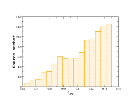
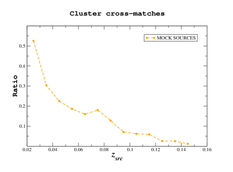
Cross-matches with catalogs of groups and clusters of galaxies shows a clear dependence. As shown in Fig. 1, we built a sample of 9800 random positions in the SDSS footprint and cross-matched it with the T12 catalog. The redshift distribution of mock sources rises up to 0.15 as those of FRICAT and FRIICAT.
The fraction of mock sources per redshift bin of size 0.01 having a positive crossmatch with a group or a cluster of galaxies within 2 Mpc, computed a its , and having 0.005 and , significantly decreases while increases. This indicates that we could expect a higher chance of finding a low redshift RG associated with a group or a galaxy cluster than a high redshift one. Thus we chose the thresholds on the number of cosmological neighbors in the cosmological overdensity as function of .
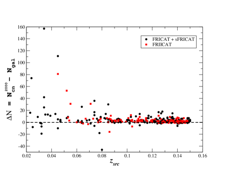
A second problem arises when using catalog crossmatches regarding the richness estimated. In Fig. 2 we show the difference between the number of cosmological neighbors, lying within 2 Mpc distance from the central RG and from the T12 group/cluster catalog. It is quite evident that the parameter underestimates the group/cluster richness. There are only a few cases where provides a lower estimate of the group/cluster richness. However, these cases could be also due to an incorrect run of the algorithm of the T12 catalog since we did not detect sources lying at similar redshift of the central RG and not even candidate elliptical galaxies for most of them. It is worth noting that the richness estimated in cluster catalogs is generally decreasing with redshift, as for example occurs for in the T12, thus expecting to find less galaxy-rich environments as increases.
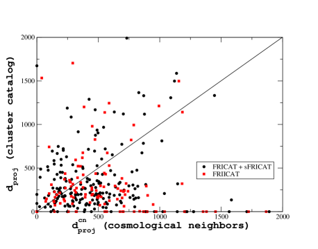
Additional advantages of the method based on the cosmological overdensity with respect to the cluster catalog crossmatches regard the estimate of the position of the central RG with respect to cluster center both in angular separation and redshift. In Fig. 3 we show the projected distance measured between the position of the RG in the center of the field examined and i) the centroid of the spatial distribution of cosmological neighbors within 2 Mpc (x-axis) or ii) that of the group/cluster reported in the T12 catalog (y-axis). The majority of sources have values below bisector indicating that estimated via cosmological neighbors tend to be smaller than those evaluated with the T12 catalog.
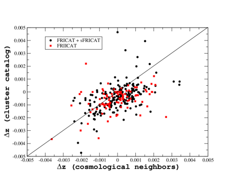
Finally, in Fig. 4 we show the redshift difference between the central RG and i) the average value of the of cosmological neighbors lying within 2 Mpc (x-axis) and ii) the redshift of the closest cluster associated using the T12 catalog (y-axis). Once again the largest fraction of RG in both FRICAT and FRIICAT lies below the bisector, highlighting that cosmological neighbors provide a better sampling of the RG large-scale environment. Assuming that all RGs belong to a galaxy group/cluster, thanks to the distribution of cosmological neighbors we can achieve a better estimate of its redshift: .
4.2. Cosmological dependences of noise
Selecting candidate elliptical galaxies on the basis of their spectroscopic redshift, whenever possible, is more precise than for example performing a simple magnitude cut as to estimate the Abell environmental richness. Counting overdensity of optical sources within a certain distance in kpc and with apparent magnitude , with being the apparent magnitude of the central radio source (see e.g., Hill & Lilly, 1991), introduces a significant amount of noise due to background and foreground objects being counted. This occurs because the number of optical galaxies increases significantly with the magnitude as shown for example in Fig. 5 for the band apparent magnitude of galaxy-type objects (i.e., uc=rc=gc=ic=zc=3) in the 2 Mpc field of the FR I SDSSJ073505.25+415827.5.
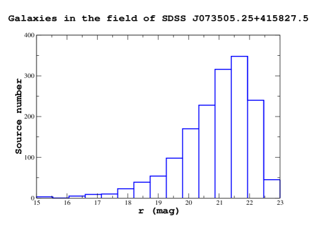
Thus comparing overdensity of optical sources around RG lying at different when having the same absolute magnitude, or simply at different apparent magnitudes, implies comparing sources with a different signal-to-noise ratio. This makes the comparison between source populations having a different redshift distribution and/or different apparent magnitude distribution and/or a similar intrinsic luminosity/absolute magnitude, as FR Is and FR IIs, challenging. This effect could be actually mitigated by counting number sources per unit of area, since at larger redshifts areas of same physical size appear smaller thus containing less background/foreground sources (i.e., less noise), but, on the other hand, it does not help since it introduces a cosmological dependence of the noise.
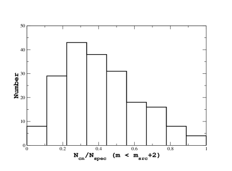
In addition, sources selected to be galaxies above a certain threshold of apparent magnitude do not necessarily belong to the same group or cluster of galaxies. In Fig. 6, we show the ratio between the total number of cosmological neighbors and that of optical sources with spectroscopic redshifts both selected to have in the band, similar to the definition of Abell classes (see e.g., Abell et al., 1989), within 2 Mpc distance from all FR Is listed in the FRICAT. Only 30-40% are generally lying at similar redshifts being so classifiable as cosmological neighbors, while others are simply background and foreground sources (i.e., noise), with very different redshifts, and thus erroneously counted.
Noise-related effects related to the source selection with certain apparent magnitude can be partially mitigated by using photometric redshift estimates, as those provided in the SDSS, and counting sources on the basis of their absolute magnitudes and color (see e.g., Blanton et al., 2000, 2001; Wing et al., 2011, and references therein), but not fully avoided. On the other hand, as shown in M19, the cosmological overdensity method does not suffer this noise effect since the threshold to indicate sources in a galaxy-rich large-scale environment is chosen as function of redshifts and because we compare RGs in the same redshift bin.
4.3. Redshift evolution of the cosmological overdensity
Here we show the underlying reason of adopting an “adaptive” procedure, as the cosmological overdensity method, with a threshold on the number of cosmological neighbors changing with redshift .
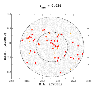
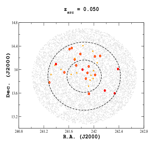
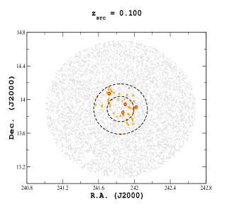
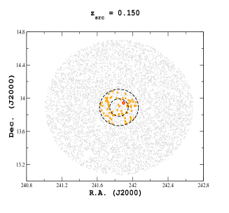
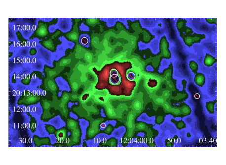
In Fig 7 we show the 2 Mpc field around the FR I SDSS J160722.95+135316.4 at 0.034, where red circles mark the locations of cosmological neighbors and dashed lines the distances of 1 Mpc and 2 Mpc, respectively. We computed the absolute magnitude in the band of all cosmological neighbors and then maintaining their intrinsic power we rescaled them at larger distances, namely at redshifts 0.05, 0.10 and 0.15. We also recomputed the radii of the circles of 500 kpc, 1 Mpc and 2 Mpc at each redshift.
In each plot of Fig 7 we only reported those cosmological neighbors having the rescaled apparent magnitude brighter than 17.8 corresponding to the SDSS criterion to select targets for spectroscopic observations. For the case of SDSS J160722.95+135316.4 the number of cosmological neighbors within 500 kpc (i.e., ) decreases from 10 at 0.034, to 3, 2 at 0.05, 0.10 and none at 0.15, resepctively, while is actually 47 at 0.034 and 20, 4, 1 at 0.05, 0.10, 0.15, respectively.
This suggests that the threshold chosen to indicate a galaxy-rich large-scale environment must be redshift dependent as we defined in our previous analysis on the basis of the MonteCarlo simulations performed on a large sample of random positions in the sky. We highlight that the above calculation does not take into account of any cosmological evolution of the groups or the clusters where RGs lie, it is a pure effect of the SDSS selection of spectroscopic targets that decreases the number of cosmological neighbors when the redshift increases as shown in our previous analysis (Massaro et al., 2019).
Finally, we also show in Fig 7 the number of optical galaxies with , to highlight how the noise increases moving at higher redshift where the absolute magnitude of the central RG is fixed and it apparent magnitude is rescaled.
5. Statistical analyses
To provide an additional evidence that the both FR Is and FR IIs live in galaxy-rich large-scale environment, we performed the following statistical tests all based on the number of cosmological neighbors surrounding them. It is worth noting that, as previously stated, the FRICAT used here is larger than the one adopted in our previous analysis since we also included the sFRICAT sample, allowing us to get a better sampling of the FR I population at lower redshifts.
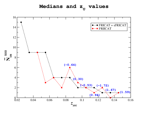
The first test is based on the median of both FR I and FR II distributions. We computed median values of for FR Is (i.e., ), per bin of of size 0.01, and then we compared the distribution of for FR IIs with . We expect that if both RG populations live in large-scale environment of similar richness, 50% of the FR IIs would lie above the median value computed for the FR Is while 50% below, for each bin of . We also applied the same test to . All medians values of both and computed for the FR I population are reported in Table 1, together with the number of FR IIs that lie above and below the medians or having the same number of cosmological neighbors, per redshift bin.
For , in all 11 bins explored, where we can compare FR Is and FR IIs, we found that in 4 cases the FR II median values are greater than computed for FR Is while in other 3 cases the situation is the opposite, and in all remaining cases medians of the two populations show the same medians. This is in agreement with the expectations of a binomial distribution, thus strengthening our results that, independently of their radio morphology, both classes of FR Is and FR IIs live in similar galaxy-rich large-scale environment. The median values for both population of FR Is and FR IIs are shown in Fig. 8. Then comparing the situation is in agreement with previous results with 5 cases for which of FR IIs is lower than that for the FR I population and 5 cases for which it is greater. Consequently, we can firmly confirm that the large-scale environments of the two classes of RGs, in each considered redshift range, is consistent.
Unfortunately, this first statistical test does not consider the two populations symmetrically, and it throws away almost all information about the distribution of environments present in the data. For example, if FR IIs has a systematically broader distribution of than FR Is, or a small tail of very rich, or very poor, environments, this first statistical test would be not sensitive to it. Thus, as second statistical check, we also applied the Mann-Whitney rank test (a.k.a. Wilcoxon-Mann-Whitney test) to each redshift bin. In Fig. 8 we also report, above each value of the medians of the two RG distributions of the normalized variable, defined as ), computed for the Mann-Whitney test and this is always consistent with zero, as expected, within 2 level of confidence, with the only exception of a single bin between and where the number for the FR IIs appears systematically lower than the median of FR Is (see Table 1). It is worth noting that we did not apply this test at 0.08 given the low number of FR IIs in these bins. Moreover, also this second statistical test is in agreement with our claim that the large-scale environments of FR Is and FR IIs cannot be distinguishable.
Then, for all redshift bins above 0.08 we also performed the two-sided Kolmogorov-Smirnov test between the distributions of and of both FR Is and FR IIs, results on the variable compute as well as correspondent -values are reported in Table 2, where in agreement with previous tests and the null hypothesis that the two distributions are the same cannot be rejected.
| 0.045 | 9 | 0 - 0 - 1 | 44 | 1 - 0 - 0 |
|---|---|---|---|---|
| 0.055 | 9 | 1 - 4 - 0 | 50 | 1 - 4 - 0 |
| 0.065 | 4 | 1 - 2 - 1 | 18 | 2 - 1 - 1 |
| 0.075 | 4 | 2 - 4 - 0 | 23 | 2 - 4 - 0 |
| 0.085 | 4 | 6 - 2 - 0 | 12 | 6 - 1 - 1 |
| 0.095 | 2 | 5 - 4 - 0 | 11 | 3 - 6 - 0 |
| 0.105 | 2 | 5 - 5 - 4 | 9 | 6 - 7 - 1 |
| 0.115 | 2 | 2 - 7 - 3 | 5 | 6 - 5 - 1 |
| 0.125 | 1 | 6 - 0 - 5 | 5 | 6 - 5 - 0 |
| 0.135 | 1 | 3 -10 - 4 | 8 | 1 -15 - 1 |
| 0.145 | 1 | 3 -14 -11 | 3 | 13 -13 - 2 |
| total | - | 34 - 52 - 29 | - | 47 - 61 - 7 |
Note: col. (1) report the central value of each redshift bin while col. (2) and col. (4) median values for the and parameters computed for the FR I population and in comparison with the number of FR IIs (i.e., ) lying above (), below () these median values of having being the same () as shown in col. (3) and col. (5), respectively.
Finally, we verified that the shape of the two distributions with a third statistical check computing the skewness and the Pearson median skewness and verifying that the sign of both these parameters corresponds. This occurs in all redshift bins above 0.1 while below, due to the poor number of FR II radio galaxies in each bin strongly affects both parameters providing not significant results. Again this last test provide results in agreement with the previous ones.
| D() | p() | D() | p() | |
|---|---|---|---|---|
| 0.085 | 0.289 | 0.804 | 0.337 | 0.629 |
| 0.095 | 0.291 | 0.760 | 0.368 | 0.469 |
| 0.105 | 0.232 | 0.816 | 0.223 | 0.851 |
| 0.115 | 0.172 | 0.986 | 0.235 | 0.831 |
| 0.125 | 0.296 | 0.499 | 0.269 | 0.622 |
| 0.135 | 0.224 | 0.650 | 0.382 | 0.084 |
| 0.145 | 0.205 | 0.445 | 0.089 | 0.999 |
Note: col. (1) report the central value of each redshift bin, while col. (2) and col. (4) the statistical variable and col. (3) and col.(5) the correspondent -value for the distribution of and , respectively.
6. Environmental properties
6.1. Environmental parameters: definition
On the basis of the distribution of the cosmological neighbors it is possible to estimate several parameters to investigate the properties of the large-scale environments surrounding FR Is and FR IIs and compare them with those of the central RGs.
In particular, we defined the following quantities.
-
•
The concentration parameter . It is defined as the ratio of the number of cosmological neighbors lying within 500 kpc and those within 1 Mpc. This parameter allows us to test if the RG tends to lie close to the center of the group or clusters of galaxies around it or in its outskirt. A similar concentration parameter has been estimate using candidate elliptical galaxies rather than cosmological neighbors: .
-
•
The average projected distance of the distribution of cosmological neighbors computed between their position and that of the central RG.
-
•
The standard deviation of the redshift distribution of the cosmological neighbors surrounding each RG.
All values for the environmental parameters described above are also reported in Table 3 in Appendix.
6.2. Environmental parameters: statistical analysis
We investigated the distribution of the environmental parameters previously defined searching for possible trends with the RG properties, such as the absolute magnitude in the band , the radio luminosity and the [OIII] emission line luminosity .
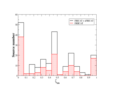
The distribution of the concentration parameter for both FRICAT and FRIICAT is shown in Fig. 9. There are 52 FR Is out of 209 and 34 FR IIs out of a total 115, that have no cosmological neighbors within 500 kpc distance from their position. However this does not imply that their large-scale environment is not rich since it could be due, for example, to the SDSS spectroscopic incompleteness and/or to the position of the RG in the outskirt of its galaxy-rich large-scale environment. Most of the remaining RGs indeed appear to inhabit an environment with high galaxy density.
We note that the distribution of sources around a random position in the sky follows, in general, a uniform distribution, where the number of sources is expected to scale as , with being the angular separation from the random position. Thus assuming that the same situation could be applicable to cosmological neighbors, the expected value of the is 0.25 while the largest fraction of the observed values is significantly higher.
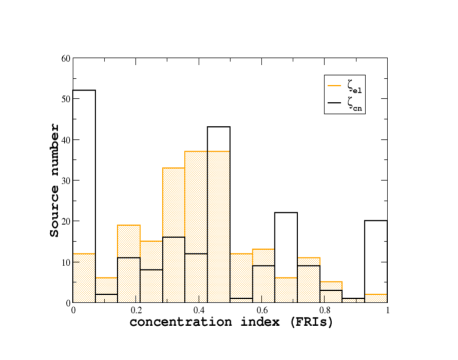
In Fig. 10 we show the comparison between the concentration indices of FR Is computed using the number of cosmological neighbors and that of candidate elliptical galaxies . The distribution of is peaking around 0.4 and has the largest fraction of values in the range 0.2-0.6. There are less values around zero since it is “easier” to find candidate elliptical galaxies than cosmological neighbors due to the SDSS fiber cladding, which prevents fibers from being placed closer than 55″. A similar situation occurs for FR IIs.
We conclude that, independently of the concentration parameter adopted, RGs appear to inhabit galaxy-rich large-scale environments lying closer to the centroid of both cosmological neighbors and candidate elliptical galaxies.
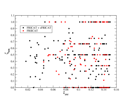
Moreover, in Fig. 11 we also report the value of as function of the source redshift . We do not see any trend/correlation between these two parameters and not even differences between the two RG classes.
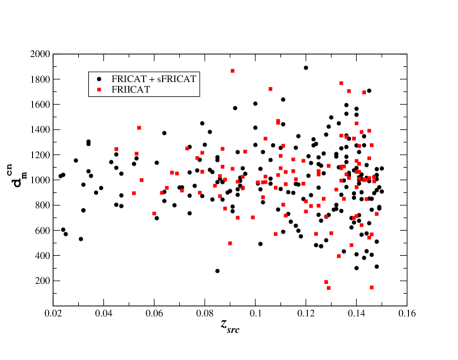
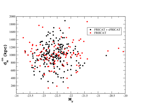
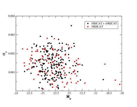
Then we explore the distribution of the average projected distance of the distribution of cosmological neighbors and the standard deviation of their redshift distribution. These parameters provide an estimate of the group/cluster physical size.
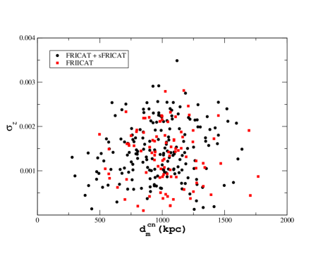
Their comparison is shown in Fig. 12. We did not find any trend between these two parameters for both classes of RGs and as shown by their distributions in Fig. 13. In the latter case, we carried out a two-sided Kolmogorov-Smirnov test and we found the parameter equal to 0.113 and corresponding to a -value of 0.395 for a total number of 186 values of for the FR Is and 96 for the FR IIs, thus indicating that the null hypothesis that the two distributions are the same cannot be rejected.
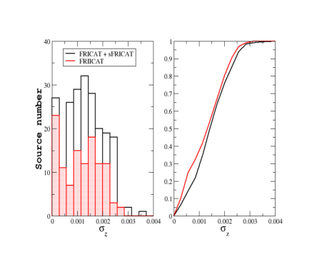
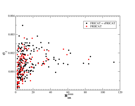
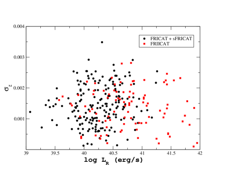
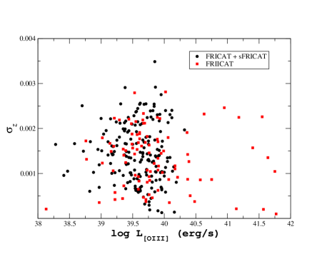
However, as shown in Fig. 14, we found that for high values of the redshift dispersion appear clustered around the 0.002.
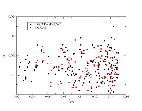
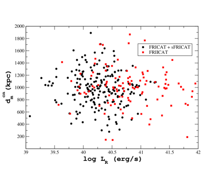
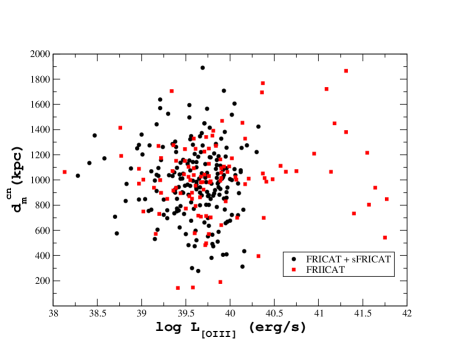
In Fig. 15 we also show the values of both parameters, and , as function of but no evidence of any trend is found.
Finally, we explored other links between parameters of the central RG and those of the surrounding environments but no neat trends are evident. Figures are shown in Appendix.
We show and in comparison with the absolute magnitude in the band of the RG where no trend/link is identified. A similar situation occurs also when comparing both these environmental parameters with radio power and emission line luminosity of the [OIII], i.e., . The plot with allows us also to test if there are differences between LERGs and HERGs, even if given the low number of HERGs present in our sample, these results must be treated with caution making this comparison less statistically significant. We conclude that independently by the power of the central RG in different energy range or that of its host galaxy the properties of its large-scale environment is the same, being independent by the radio morphology.
7. X-ray perspectives
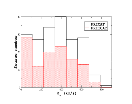
We converted the standard deviation of the redshift distribution computed using all cosmological neighbors within 2 Mpc: into an estimate of the velocity dispersion of galaxies in the large-scale environments of radio galaxies. We computed the standard deviation of the line-of-sight component of the velocity (i.e. radial velocity) according to Danese et al. (1980), thus using the following relation:
| (1) |
where is the redshift of the central radio galaxy and is the average redshift of all cosmological neighbors within 2 Mpc. In Fig. 16 we show the distribution of the velocity dispersion computed on the basis of Eq. (1).
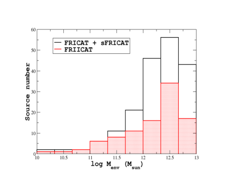
Then, considering , we also assumed that groups and clusters surrounding radio galaxies, being gravitationally bound, are virialized and thus we estimated the total mass , i.e. galaxies plus IGM plus dark matter content, for their large-scale environments, according to
| (2) |
where we assumed 2 Mpc and we neglect the form factor 3/5.
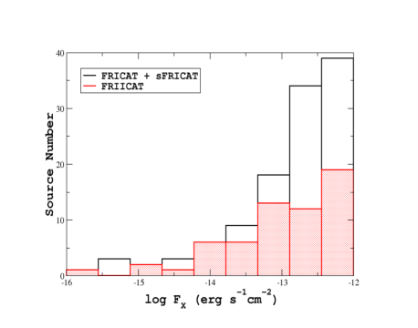
We finally adopted two different correlations to estimate the X-ray luminosity and the X-ray integrated flux . The first correlation is
| (3) |
as reported by Reiprich & Böhringer (1999) while the second directly links with the X-ray luminosity:
| (4) |
found by Clerc et al. (2016), where .
Hence in Fig. 17 we show the distribution of the environmental mass as well as that X-ray fluxes estimated according to the previous relations and, using Eq. (3), as expected, they are all below the threshold of 4.410-12 erg/cm/s of the ROSAT Brightest Cluster Sample (Ebeling et al., 1998), while the same situation occurs for more than 95% of both radio galaxy catalogs when using Eq. (4). We remark that both estimates are also consistent with those derived using the vs correlation found by Zhang et al. (2011).
X-ray detection of the IGM emission in the large-scale environments of these radio galaxies depends on several issues (e.g., distribution of the surface brightness, X-ray background, size of the galaxy cluster etc.). However assuming that the X-ray integrated flux is uniformly spread over a circular region of 500 kpc radius centered on the central radio source, the mean values of the X-ray intensity we estimated ranges between 3-4e-16 and 1e-14 for both FR Is and FR IIs, respectively; typical values of galaxy clusters detected by satellites as XMM-Newton and Chandra (see e.g., Lloyd-Davies et al., 2011; Mehrtens et al., 2012).
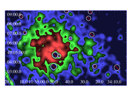
Finally, we selected 2 FR Is out of 6 radio galaxies for which X-ray observations are available in the XMM-Newton archive and we carried out a simple analysis to show that low exposure times (5 ksec) can guarantee the X-ray detection of the IGM in galaxy cluster around them as well as in the majority of the sources in explored catalogs. Selected sources are: SDSS J113359.23+490343.4 and SDSS J120401.4+201356.3 and we cut the exposure times of their archival datasets to 5.5 ksec.
EPIC data were retrieved from the XMM-Newton Science Archive111http://nxsa.esac.esa.int/nxsa-web and reduced with the SAS222http://www.cosmos.esa.int/web/XMM-Newton/sas 16.1.0 software. Following Nevalainen et al. (2005), we filtered XMM data for hard-band flares by excluding the time intervals where the high energy ( keV for MOS1 and MOS1, keV for PN) count rate evaluated on the whole detector FOV was more than 3 away from its average value. To achieve a tighter filtering of background flares, we iteratively repeated this process two more times, re-evaluating the average hard-band count-rate and excluding time intervals away more than 3 from this value. The same procedure was applied to soft keV band restricting the analysis to an annulus with inner and outer radii of 12’ and 14’, where the emission from the radio galaxy is expected to be small.
We merged data from MOS1, MOS2 and PN detectors from all observations using the merge task, to detect the fainter sources that would not be detected otherwise. Sources were detected on these merged images following the standard SAS sliding box task edetect_chain that mainly consist of three steps: (i) source detection with local background, with a minimum detection likelihood of 8; (ii) remove sources in step 1 and create a smooth background maps by fitting a 2-D spline to the residual image; (iii) source detection with the background map produced in step 2 with a minimum detection likelihood of 10.
The task emldetect was then used to determine the parameters for each input source by means of a maximum likelihood fit to the input images, selecting sources with a minimum detection likelihood of 15 and a flux in the keV band larger than (assuming an energy conversion factor of ). An analytical model of the point spread function (PSF) was evaluated at the source position and normalized to the source brightness. The source extent was then evaluated as the radius at which the PSF level equals half of local background. We finally visually inspected the detected sources and removed evident spurious detections (i. e., at chip borders, in regions of diffuse emission, etc.). We then produced “swiss-cheese” images for each detector array and observation.
As shown in the upper panels of Fig. 18 we clearly detected extended X-ray emission in the merged XMM-Newton archival images around each radio galaxy, while in the lower panels of Fig. 18 the surface brightness profiles are also reported.
It is also worth mentioning that we measured the integrated X-ray flux over a circular region of size equal to the maximum extent of the X-ray diffuse emission, evaluated by the surface brightness profiles, and it is in agreement with those values estimated using Eq. (3) and Eq.(4) for all three radio galaxies.
8. Summary and Conclusions
We recently carried out an extensive investigation of the RG large-scale environment in the local Universe (i.e., at 0.15). Our analysis was based on the comparison of different clustering algorithms and on the development of a new method, based on the counts of cosmological neighbors: optical sources lying within 2 Mpc and with a redshift difference 0.005 with respect to the RG lying at the center of the field examined, a method known as cosmological overdensity. Our study was also based on extremely homogeneous RG catalogs, with uniform radio, infrared and optical data available for all sources, allowing us to distinguish between FR I and FR II or LERG vs. HERG. We found that independently of their radio morphological classification they all appear to live in similar galaxy-rich large-scale environments. The same result, even if less statistically significant, was also obtained while investigating LERG vs HERG environments (M19).
Here we first performed a dedicated analysis to show how cosmological biases and artifacts can affect analyses of RG large-scale environments and how the cosmological overdensity is almost not affected. Then, even if our procedure is dependent by the SDSS selection of spectroscopic targets, it permits us to obtain better estimates of i) the ambient richness ii) the center of the galaxy distribution surrounding target RGs and iii) the redshift difference between central RG and the average values of cosmological neighbors, that seems to be a better estimate of the environmental redshift. We stress the importance of comparing radio sources in the same redshift bins to obtain a complete overview of their large-scale environments in particular for procedures not based on spectroscopic redshift estimates.
We also presented an additional statistical test based on the distribution of the median values of the RG population that showed, consistently with our previous analysis, how FR Is and FR IIs live in large-scale environments having environments that are indistinguishable on the basis of the statistical analysis we carried out, at all redshifts up to 0.15. The lack of a significant number of HERGs (only 14 out of 105 total RGs) listed in the FRIICAT prevent us to draw firm conclusions on the comparison between them and LERGs and thus it was not explored.
In the current paper we also investigated several properties of the RG environments on Mpc scale using the cosmological neighbors distribution and a few parameters derived. Our main results are summarized as follows.
-
1.
The concentration parameter , defined as the ratio between the number of cosmological neighbors within 500 kpc and those within 1 Mpc, does not depend by the RG redshift and has a distribution that does not depend by the radio classification (i.e., FR I vs. FR II). Typical values of are well above 0.25 expected by a uniform distribution of surrounding cosmological neighbors. Consistent results are obtained even when using the number of candidate elliptical galaxies instead of the cosmological neighbors.
-
2.
FR Is and FR IIs have also similar distributions of the standard deviation of the redshift distribution of the cosmological neighbors as well as their average projected distance computed between their position and that of the central RG. This implies that in the redshift range explored the RG environments have similar sizes.
-
3.
When comparing the properties of the cosmological neighbors with those of the central RGs, as the absolute magnitude , the radio power and emission line luminosity, we did not find any trend and any difference between FR I and FR II populations.
Finally, we used the parameter to estimate the velocity dispersion of cosmological neighbors and assume that this is the same of all galaxies belonging to the large-scale environment of both RG populations. Then under the assumption that these RG environments are virialized we estimated the total mass present therein, i.e., mass of galaxies plus IGM plus dark matter content.
Thanks to the correlations between and the X-ray luminosity of the IGM we also computed the expected values necessary to draw the feasibility of future X-ray campaigns and/or pave the path to what eROSITA will be able to detect in the near future. Given the same distribution of and the lack of any trend with this parameter with those of the central radio galaxies (i.e., , and ) the same situation occurs with the derived quantities: and of their large-scale environments. However, the estimates of X-ray fluxes confirm that X-ray counterpart of the groups and clusters of galaxies around FRICAT and FRIICAT sources should not to be detected in the ROSAT all sky survey demanding to XMM-Newton and Chandra facilities to get a complete view of their large-scale environments. Finally, we reduced and analyzed XMM-Newton observations of two FR I radio galaxies, cutting the total exposure time to 5.5 ksec, to show that a clear detection of galaxy clusters around them can be easily achieved with snapshot observations.
Appendix A Figures & Tables
We did not find any trend between the environmental parameters: and radio galaxy parameters as , , , but all plots are indeed shown in this Appendix A in Fig. 19, Fig. 20 and Fig. 21, respectively.
We then reported here in Table 3 all parameters estimated for each RG analyzed.
| SDSS | Radio | ||||||||||||||
|---|---|---|---|---|---|---|---|---|---|---|---|---|---|---|---|
| name | Class | (kpc) | (kpc) | (kpc) | (km/s) | erg/cm2s-1 | |||||||||
| J073014.37+393200.4 | FRI | 0.142 | 5.3E-4 | 450.42 | 1 | 4 | 6 | 0.25 | 0.141 | 0.00082 | 207.56 | 902.48 | 215.61 | 11.86 | -13.18 |
| J073505.25+415827.5 | FRI | 0.087 | 5.2E-4 | 161.92 | 3 | 4 | 10 | 0.75 | 0.088 | 0.00061 | 758.00 | 985.60 | 168.04 | 11.64 | -13.05 |
| J073719.18+292932.0 | FRI | 0.111 | 8.1E-4 | 159.92 | 1 | 1 | 5 | 1.00 | 0.108 | 0.00161 | 826.91 | 1441.76 | 436.15 | 12.47 | -12.07 |
| J074125.85+480914.3 | FRI | 0.12 | - | - | 0 | 0 | 1 | - | 0.115 | - | 1890.54 | 1890.55 | - | - | - |
| J074351.25+282128.0 | FRI | 0.106 | 3.0E-4 | 63.64 | 4 | 4 | 9 | 1.00 | 0.106 | 0.00211 | 258.80 | 1010.41 | 572.42 | 12.71 | -11.69 |
| J075221.83+333348.9 | FRII | 0.14 | 1.7E-4 | 111.63 | 2 | 2 | 4 | 1.00 | 0.138 | 0.00143 | 140.75 | 943.39 | 375.43 | 12.34 | -12.47 |
| J075309.91+355557.1 | FRI | 0.113 | 4.5E-4 | 180.50 | 2 | 4 | 5 | 0.50 | 0.113 | 0.00097 | 229.58 | 730.53 | 260.57 | 12.02 | -12.73 |
| J075506.67+262115.9 | FRI | 0.123 | - | - | 0 | 0 | 1 | - | 0.123 | - | 1274.66 | 1274.66 | - | - | - |
| J075529.95+520450.6 | FRII | 0.14 | - | - | 0 | 0 | 0 | - | - | - | - | - | - | - | - |
| J075628.78+501716.3 | FRII | 0.134 | - | - | 0 | 0 | 2 | - | 0.133 | 0.00087 | 322.70 | 1768.24 | 230.16 | 11.91 | -13.04 |
Col. (1): SDSS name.
Col. (2): Radio class to distinguish between source belonging to the FRICAT and the FRIICAT.
Col. (3): source redshift.
Col. (4): Absolute value of the redshift difference between the RG and the closest galaxy cluster in the T12 catalog.
Col. (5): Physical distance between the RG and the closest galaxy cluster in the T12 catalog. This is computed at the of the central RG.
Col. (6,7,8): Number of cosmological neighbors within 500, 1000 ad 2000 kpc, respectively, estimated at the of the central radio galaxy.
Col. (9): The concentration parameter .
Col. (10): The average redshift of the cosmological neighbors in 2 Mpc.
Col. (11): The standard deviation of the redshift distribution for the cosmological neighbors within 2 Mpc.
Col. (12): Physical distance between the central RG and the average position of the cosmological neighbors within 2 Mpc. This is computed at the of the central RG.
Col. (13): Average distance of the cosmological neighbors within 2 Mpc.
Col. (14): Velocity dispersion of the cosmological neighbors located in 2 Mpc.
Col. (15): Environmental mass estimated from the velocity dispersion.
Col. (16): X-ray flux estimated from the velocity dispersion.
References
- Abell et al. (1989) Abell, G. O., Corwin, H. G. Jr., Olowin, O. P. 1989 ApJS, 70, 1
- Ahn et al. (2012) Ahn, C. P., Alexandroff, R., Allende Prieto, C., Anderson, Scott F., Anderton, T. et al. 2012 ApJS, 203, 21
- Baldi et al. (2015) Baldi, Ranieri D.; Capetti, Alessandro; Giovannini, Gabriele 2015 A&A, 576A, 38
- Baldi et al. (2018) Baldi, R. D.; Capetti, A.; Massaro, F. 2018 A&A, 609A, 1
- Belsole et al. (2007) Belsole, E.; Worrall, D. M.; Hardcastle, M. J.; Croston, J. H. 2007 MNRAS 381, 1109
- Bennett et al. (2014) Bennett, C. L., Larson, D., Weiland, J. L., Hinshaw, G. 2014 ApJ 794, 135
- Berlind et al. (2006) Berlind, A. A. et al. 2006 ApJS, 167, 1
- Best (2004) Best, P. N. 2004 MNRAS 351, 70
- Best & Heckman (2012) Best, P. N.; Heckman, T. M. 2012 MNRAS 421, 1569
- Biviano (2000) Biviano A. 2000 IAP meeting “Constructing the Universe with Clusters of Galaxies”, Paris, France, July 2000, Florence Durret & Daniel Gerbal Eds.,
- Blanton et al. (2000) Blanton, E. L.; Gregg, M. D.; Helfand, D. J.; Becker, R. H.; White, R. L. 2000 ApJ, 531, 118
- Blanton et al. (2001) Blanton, E. L.; Gregg, M. D.; Helfand, D. J.; Becker, R. H.; Leighly, K. M. 2001 AJ, 121, 2915
- (13) Capetti, A., Massaro, F., Baldi, R. D. 2017 A&A 598A, 49
- (14) Capetti, A., Massaro, F., Baldi, R. D. 2017 A&A 601A, 81
- Ching et al. (2017) Ching, J. H. Y.; Croom, S. M.; Sadler, E. M.; Robotham, A. S. G.; Brough, S. et al. 2017 MNRAS 469, 4584
- Clerc et al. (2016) Clerc, N.; Merloni, A.; Zhang, Y. -Y.; Finoguenov, A.; Dwelly, T. et al. 2016 MNRAS 463, 4490
- Condon et al. (1998) Condon, J. J., Cotton, W. D., Greisen, E. W., Yin, Q. F., Perley, R. A., Taylor, G. B., & Broderick, J. J. 1998, AJ, 115, 1693
- Croston et al. (2008) Croston, J. H.; Hardcastle, M. J.; Birkinshaw, M.; Worrall, D. M.; Laing, R. A. 2008 MNRAS, 386, 1709
- Danese et al. (1980) Danese, L., de Zotti, G., di Tullio, G., 1980 A&A, 82, 322
- D’Abrusco et al. (2009) D’Abrusco, R.; Longo, G.; Walton, N. A. 2009 MNRAS 396, 223
- D’Agostini (2003) D’Agostini, G. 2003 “Bayesian reasoning in data analysis: A critical introduction”, World Scientific Publishing, 2003
- Ebeling et al. (1998) Ebeling, H.; Edge, A. C.; Bohringer, H.; Allen, S. W.; Crawford, C. S.; Fabian, A. C.; Voges, W.; Huchra, J. P. 1998 MNRAS 301, 881
- Eke et al. (2004) Eke, V. R 2004 MNRAS, 348, 866
- Evans et al. (2006) Evans, D. A.; Worrall, D. M.; Hardcastle, M. J.; Kraft, R. P.; Birkinshaw, M. 2006 ApJ, 642, 96
- Fadda et al. (1996) Fadda, D.; Girardi, M.; Giuricin, G.; Mardirossian, F.; Mezzetti, M. 1996 ApJ, 473, 670
- Fanaroff & Riley (1974) Fanaroff, B. L, Riley, J. M. 1974 MNRAS 167, 31
- Gendre et al. (2013) Gendre M. A., Best, P. N., Wall, J. V. and Ker, L.M. 2013 MNRAS 430, 3086
- Girardi et al. (1993) Girardi, M.; Biviano, A.; Giuricin, G.; Mardirossian, F.; Mezzetti, M. 1993 ApJ, 404, 38
- Gladders et al. (1998) Gladders, M. D., Lopez-Cruz, O., Yee, H. K. C. & Kodama, T. 1998, ApJ, 501, 571
- Gladders et al. (2000) Gladders, Michael D.; Yee, H. K. C. 2000 ApJ 120, 2148
- Haas et al. (2012) Haas, M. R., Schaye, J., Jeeson-Daniel, Akila 2012 MNRAS 419, 2133
- Hardcastle & Worrall (2000) Hardcastle, M. J.; Worrall, D. M. 2000 MNRAS, 319, 562
- Helfand et al. (2015) Helfand, D. J., White, R. L., Becker, R. H. 2015 ApJ, 801,26
- Hill & Lilly (1991) Hill, G. J. and Lilly, S. J. 1991 ApJ 367, 1
- Hine & Longair (1979) Hine, R. G.; Longair, M. S. 1979 MNRAS 188, 111
- Hucra & Geller (1982) Huchra J. P., Geller M. J., 1982, ApJ, 257, 423
- Ineson et al. (2013) Ineson, J.; Croston, J. H.; Hardcastle, M. J.; Kraft, R. P.; Evans, D. A.; Jarvis, M. 2013 ApJ 770, 136
- Ineson et al. (2015) Ineson, J.; Croston, J. H.; Hardcastle, M. J.; Kraft, R. P.; Evans, D. A.; Jarvis, M. 2015 MNRAS 453, 2682
- Laing et al. (1994) Laing, R. A.; Jenkins, C. R.; Wall, J. V.; Unger, S. W. 1994 The First Stromlo Symposium: The Physics of Active Galaxies. ASP Conference Series, Vol. 54, 1994, G.V. Bicknell, M.A. Dopita, and P.J. Quinn, Eds., p.201
- Lintott et al. (2008) Lintott, C. J., Schawinski, K., Slosar, A., Land, K., Bamford, S. et al. 2008 MNRAS 389, 1179
- Lloyd-Davies et al. (2011) Lloyd-Davies, E. J.; Romer, A. Kathy; Mehrtens, Nicola; Hosmer, Mark; Davidson, Michael et al. 2011 MNRAS 418, 14
- Massaro et al. (2011) Massaro, F., D’Abrusco, R., Ajello, M. et al. 2011 ApJ, 740L, 48
- Massaro et al. (2012) Massaro, F., Tremblay, G. R., Harris, D. E. et al. 2012 ApJS, 203, 31
- Massaro et al. (2013) Massaro, F., D’Abrusco, R., Paggi, A. et al. 2013a ApJS, 209, 10
- Massaro et al. (2015) Massaro, F., Harris, D. E., Liuzzo, E. et al. 2015 ApJS, 220, 5
- Massaro et al. (2018) Massaro, F., Missaglia, V., Stuardi, C., Harris, D. E., Kraft, R. P. et al. 2018 ApJS, 234, 7
- Massaro et al. (2019) Massaro, F., N. Álvarez-Crespo, N., Capetti, A., Baldi, R. D., Pillitteri, I., Campana, R., Paggi, A., 2019 ApJS, 240, 2
- Mehrtens et al. (2012) Mehrtens, Nicola; Romer, A. Kathy; Hilton, Matt; Lloyd-Davies, E. J.; Miller, Christopher J. et al. 2012 MNRAS 423, 1024
- Mingo et al. (2014) Mingo, B.; Hardcastle, M. J.; Croston, J. H.; Dicken, D.; Evans, D. A.; Morganti, R.; Tadhunter, C. 2014 MNRAS, 440, 269
- Mingo et al. (2017) Mingo, B.; Hardcastle, M. J.; Ineson, J.; Mahatma, V.; Croston, J. H.; Dicken, D.; Evans, D. A.; Morganti, R.; Tadhunter, C. 2017 MNRAS, 470, 2762
- Miraghei & Best (2017) Miraghaei, H. and Best, P. N. 2017 MNRAS 466 4346
- Moore et al. (1993) Moore, B., Frenk, C. S., White, S. D. M. 1993 MNRAS, 261, 827
- Nevalainen et al. (2005) Nevalainen, J.; Markevitch, M.; Lumb, D. 2005 ApJ 629, 172
- Prestage & Peacock (1988) Prestage, R. M.; Peacock, J. A. 1988 MNRAS 230, 131
- Reiprich & B’́ohringer (1999) Reiprich, T. H., B’́ohringer H. 1999 AN, 320, 296
- Richards et al. (2004) Richards, Gordon T.; Nichol, Robert C.; Gray, Alexander G.; Brunner, Robert J.; Lupton, Robert H. et al. 2004 ApJS 155, 257
- Rines et al. (2013) Rines, Kenneth; Geller, Margaret J.; Diaferio, Antonaldo; Kurtz, Michael J. 2013 ApJ, 767, 15
- Sabater et al. (2013) Sabater, J.; Best, P. N.; Argudo-Fernàndez, M. 2013 MNRAS 430 ,638
- Stuardi et al. (2018) Stuardi, C., Missaglia, V., Massaro, F., Ricci, F., Liuzzo, E. et al. 2018 ApJS, 235, 32
- Tago et al. (2010) Tago, E.; Saar, E.; Tempel, E.; Einasto, J.; Einasto, M.; Nurmi, P.; Heinämäki, P. 2010 A&A, 514A, 102
- Taylor (2005) Taylor M. B., 2005, ASPC, 347, 29
- Tasse et al. (2008) Tasse, C.; Best, P. N.; Röttgering, H.; Le Borgne, D. 2008 A&A, 490, 893
- Tempel et al. (2012) Tempel, E.; Tago, E.; Liivamägi, L. J. 2012 A&A 540A,106
- (64) Visvanathan, N., & Sandage, A. 1977, ApJ, 216, 214
- White et al. (1997) White, R. L., Becker, R. H., Helfand, D. J.; Gregg, M. D. 1997 ApJ 475, 479
- Wilkes et al. (2013) Wilkes, Belinda J.; Kuraszkiewicz, Joanna; Haas, Martin; Barthel, Peter; Leipski, Christian; Willner, S. P. et al. 2013 ApJ, 773, 15
- Wing et al. (2011) Wing, Joshua D.; Blanton, Elizabeth L. 2011 AJ 141, 88
- Worpel et al. (2013) Worpel, Hauke; Brown, Michael J. I.; Jones, D. Heath; Floyd, David J. E.; Beutler, Florian 2013 ApJ 772, 64
- Worrall & Birkinshaw (2000) Worrall, D. M.; Birkinshaw, M. 2000 ApJ, 530, 719
- Wright et al. (2010) Wright, E. L., et al. 2010 AJ, 140, 1868
- Zhang et al. (2011) Zhang, Y. Y., Andernach, H., Caretta, C. A., Reiprich, T. H., B’́ohringer, H., Puchwein, E., Sijacki, D. & Girardi, M. 2011 A&A, 526, A105
- Zirbel (1997) Zirbel, E. L. 1997 ApJ 476, 489