Responsive Parallelism with Futures and State

Abstract.

Motivated by the increasing shift to multicore computers, recent work has developed language support for responsive parallel applications that mix compute-intensive tasks with latency-sensitive, usually interactive, tasks. These developments include calculi that allow assigning priorities to threads, type systems that can rule out priority inversions, and accompanying cost models for predicting responsiveness. These advances share one important limitation: all of this work assumes purely functional programming. This is a significant restriction, because many realistic interactive applications, from games to robots to web servers, use mutable state, e.g., for communication between threads.

In this paper, we lift the restriction concerning the use of state. We present $\lambda^{4}_{i}$, a calculus with implicit parallelism in the form of prioritized futures and mutable state in the form of references. Because both futures and references are first-class values, $\lambda^{4}_{i}$ programs can exhibit complex dependencies, including interaction between threads and with the external world (users, network, etc). To reason about the responsiveness of $\lambda^{4}_{i}$ programs, we extend traditional graph-based cost models for parallelism to account for dependencies created via mutable state, and we present a type system to outlaw priority inversions that can lead to unbounded blocking. We show that these techniques are practical by implementing them in C++ and present an empirical evaluation.

1. Introduction

Advances of the past decade have brought multicore computers to the mainstream. Many computers today, from a credit-card-size Raspberry Pi with four cores to a rack server, are built with multiple processors (cores). These developments have led to increased interest in languages and techniques for writing parallel programs with cooperative threading. In cooperative threading, the user expresses parallelism at a high level and a language-supplied scheduler manages parallelism at run time. Many languages, libraries, and systems for cooperative threading have been developed, including MultiLisp (Halstead, 1984), NESL (Blelloch et al., 1994), dialects of Cilk (Frigo et al., 1998; Danaher et al., 2008; Leiserson, 2010; Singer et al., 2019a), OpenMP (OpenMP 5.0, 2018), Fork/Join Java (Lea, 2000), dialects of Habanero (Barik et al., 2009; Cavé et al., 2011; Imam and Sarkar, 2014), TPL (Leijen et al., 2009), TBB (Intel, 2011), X10 (Charles et al., 2005), parallel ML (Fluet et al., 2008, 2011; Sivaramakrishnan et al., 2014; Raghunathan et al., 2016; Guatto et al., 2018), and parallel Haskell (Keller et al., 2010; Kuper et al., 2014).

Cooperative threading is well suited for compute-intensive jobs and may be used to maximize throughput by finishing a job as quickly as possible. But modern applications also include interactive jobs where a thread may needed to be completed as quickly as possible. For such interactive applications, the main optimization criterion is responsiveness — how long each thread takes to respond to a user. To meet the demands of such applications, the systems community has developed competitive threading techniques, which focus on hiding the latency of blocking operations by multiplexing independent sequential threads of control (Hauser et al., 1993; Flautner et al., 2000; Blake et al., 2010; Gao et al., 2014).

Historically, collaborative and competitive threading have been researched largely separately. With the mainstream availability of parallel computers, this separation is now obsolete: many jobs today include both compute-intensive tasks and interactive tasks. In fact, applications such as games, browsers, design tools, and all sorts of interesting interactive systems involve both compute-heavy tasks (e.g., graphics, AI, statistics calculations) and interaction. Researchers have therefore started bridging the two worlds. Muller et al. (2017, 2018, 2019) have developed programming-language techniques that allow programmers to write cooperatively threaded programs and also assign priorities to threads, as in competitive threading. By using a type system (Muller et al., 2018) and a cost model, the authors present techniques for reasoning about the responsiveness of parallel interactive program.

All of this prior work has made some progress on bridging collaborative and competitive threading, but it makes an important assumption: pure functional programming. Specifically, the work does not allow for memory effects, which are crucial for allowing threads to communicate. This restriction can be significant, because nearly all realistic interactive applications rely on mutable state and effects. As an example, consider a basic server consisting of two entities: a high-priority event loop handling queries from a user and a low-priority background thread for optimizing the server’s database. Under Muller et al.’s work, the event loop and background thread can only communicate by synchronizing, but such a synchronization would lead to a priority inversion. If effects were allowed, then the threads could communicate by using a piece of shared state.

In this paper, we overcome this restriction by developing programming language support for collaborative and competitive threading in the presence of state. To this end, we consider $\lambda^{4}_{i}$, a core calculus for an implicitly parallel language with mutable state in the form of references. The parallel portion of the calculus is based on futures, which represent asynchronous computations as first-class values. Futures can be created and synchronized in a very general fashion. The calculus also allows programmers to assign priorities to futures, which represent their computational urgency. Because it combines futures and state, $\lambda^{4}_{i}$ is very expressive and enables writing conventional nested-parallel programs as well as those with more complex and dynamic dependencies. For example, we can parallelize a dynamic-programming algorithm by creating an initially empty array of future references and then populating the array by creating futures, which may all be executed in parallel. Similarly, we can express rich interactive computations, e.g., a network event can be delegated to a future that sends asynchronous status updates via a piece of shared state implemented as a reference.

The high degree of expressiveness in $\lambda^{4}_{i}$ makes it tricky to reason about the cost due to priority inversions and non-determinism due to scheduling: because of the presence of state, the computation may depend on scheduling decisions. For these reasons, traditional graph-based cost models of parallel computations (Blelloch and Greiner, 1995, 1996; Spoonhower et al., 2008) do not apply to programs that mix futures and state. Such models typically do not take priorities into account and assume that scheduling does not change the computation graph.

We tackle these challenges by using a combination of algorithmic and formal techniques. On the algorithmic side, we extend traditional graph-based cost models to include information about priorities as well as “happens-before” edges that capture certain dependencies by reifying execution-dependent information flow through mutable state. We then prove that if a computation graph has no priority inversions, then it can be scheduled by using an extension of greedy scheduling with priorities to obtain provable bounds on the response time of any thread (Theorem 2.3). Priority inversions are not simple to reason about, so we present a type system for $\lambda^{4}_{i}$ that guarantees that any well-typed program has no priority inversions. To establish the soundness of the type system (Theorem 3.7), we model the structure of the computation by giving a dynamic semantics that, in addition to evaluating the program, creates a computation graph that captures both traditional dependencies between threads and also non-traditionally captures certain happens-before dependencies to model the impact of mutable state on the computation.

Because $\lambda^{4}_{i}$ is a formal system, it can in principle be implemented in many different languages. For this paper, we chose to implement such a system in the context of C/C++ because many real-world interactive applications with stringent performance requirements are written in C/C++. Specifically, we have developed I-Cilk, a task parallel platform that supports interactive parallel applications. I-Cilk is based on Cilk, a parallel dialect of C/C++. As with traditional cooperative threading systems, I-Cilk consists of a runtime scheduler that dynamically creates threads and maps them onto available processing cores. Unlike traditional task-parallel platforms, however, I-Cilk supports competitive threading by allowing the programmer to specify priorities of tasks. Perhaps somewhat unexpectedly, I-Cilk also includes an implementation of the $\lambda^{4}_{i}$ type system to rule out priority inversions. The type system is implemented by using inheritance, template programming, and other features of C++ to encode the restrictions necessary to prevent priority inversions. Because C++ is not a safe language, this implementation of the type system expects the programmer to obey certain conventions.

The thread scheduler of I-Cilk aims to implement the scheduling principle that Theorem 2.3 relies on. This is challenging to do efficiently because it requires maintaining global information within the scheduler that can only be achieved via frequent synchronizations. Instead, I-Cilk approximates optimal scheduling by utilizing a two-level adaptive scheduling strategy that re-evaluates the scheduling decision at a fixed scheduling quantum.

We empirically evaluate I-Cilk using three moderately-sized application benchmarks (about 1K lines each). These applications fully utilize the features of I-Cilk (including I/O and prioritization of tasks). We will dive into one application in detail to illustrate the use of future references and mutable states. To demonstrate the efficiency of I-Cilk, we compare the response times and execution times of tasks at different priority levels running on I-Cilk and on a baseline system that behaves like I-Cilk but does not account for priority. Empirically we demonstrate that indeed I-Cilk provides much better response time, illustrating the efficacy of its scheduler.

In summary, the contributions of this paper include:

• a cost model for imperative parallel programs that incorporates scheduler-dependence through mutable state (Section 2);

• a calculus $\lambda^{4}_{i}$ for imperative parallel programs, equipped with a type system that guarantees absence of priority inversions (Section 3);

• I-Cilk, a C/C++-based task parallel platform that supports interactive parallel applications with a type system and scheduler that embody the ideas of the threading model, type system, and cost model of $\lambda^{4}_{i}$ (Section 4); and

• an empirical evaluation of I-Cilk using three large case studies written with I-Cilk (Section 5).

2. A DAG Model for Responsiveness

2.1. Preliminaries

For the purpose of this paper, we will consider programs with first-class threads that implement futures. Because our models and scheduling algorithms are largely independent of the language mechanisms by which threads are created, we will simply refer to “threads” here. We assign threads a priority, written $\rho$, drawn from a partially ordered set $R$, where  $\rho_{1}\preceq\rho_{2}$ means that priority $\rho_{1}$ is lower than priority $\rho_{2}$ or $\rho_{1}=\rho_{2}$. We write $\rho_{1}\prec\rho_{2}$ for the strict partial-order relation that does not allow for reflexivity. Note that a total order is a partial order by definition and threads can be given priorities from a totally ordered set, e.g., integers.

Threads interact with each other in two ways. First, a thread $a$ may create a thread $b$, after which the two threads run in parallel. We call this operation, which returns a handle to $b$, “future-create” or simply fcreate. Second, a thread $a$ may wait for a thread $b$ to complete before proceeding. We call this operation “future-touch” or ftouch. This model subsumes the classic fork-join (spawn-sync) parallelism.

As is traditionally done, we can represent the execution of a parallel program with a Directed Acyclic Graph or a DAG. A vertex of the DAG represents an operation (without loss of generality, we will assume that a single vertex represents a uniform unit of computation time, such as a processing core cycle). A directed edge from $u$ to $u^{\prime}$, written $(u,u^{\prime})$, indicates that the operation represented by $u^{\prime}$ depends on the operation represented by $u$. We write $u\sqsupseteq u^{\prime}$ to mean that $u$ is an ancestor of $u^{\prime}$, i.e., there is a (directed) path from $u$ to $u^{\prime}$ (it may be that $u=u^{\prime}$). If it is the case that $u\not\sqsupseteq u^{\prime}$ and $u^{\prime}\not\sqsupseteq u$, then $u$ and $u^{\prime}$ may run in parallel.

A schedule of a DAG is an assignment of vertices to processing cores at each time step during the execution of a parallel program. Schedules must obey the dependences in the DAG: a vertex may only be assigned to a core if it is ready, that is, if all of its (proper) ancestors have been assigned on prior time steps. The goal of an efficient scheduler for parallel programs is to construct as short a schedule as possible. Constructing an optimal schedule is impossible when, as in many real programs, the DAG unfolds dynamically during execution and is not known ahead of time (even a relaxed offline version of the problem in which the DAG is known ahead of time is NP-hard (Ullman, 1975)). However, prior results have shown that schedules obeying certain scheduling principles are within a constant factor of optimal length while making decisions based only on information available online (i.e., they need only know the set of ready vertices at any point in time). One such scheduling principle for DAGs with priorities is prompt scheduling. At each time step, a prompt schedule assigns to a core a ready vertex $u$ such that no currently unassigned vertex is higher-priority than $u$ repeatedly until no cores remain or no ready vertices remain.

2.2. Weak Edges

Traditionally, cost models for parallel programs assume that scheduling does not change the DAG of a parallel computation. This assumption is reasonable for deterministic programs and provides a nice layer of abstraction over scheduling — we can assume that any schedule of a DAG corresponds to a valid execution. This fundamental assumption breaks in our setting where threads are first class values and state can be used to communicate in an unstructured fashion, leading to determinacy races.

Consider as an example the following program.

⬇

1thread t = NULL;

2

3void g() {}

4void f() {

5 t = fcreate(g);

6}

⬇

1void main() {

2 fcreate(f);

3 if (t != NULL) {

4 ftouch(t);

5 }

6}

(a)

(b)

(c)

Figure 1. DAGs in which the main thread reads a valid thread handle (a) and NULL (b), and a DAG with a weak edge representing a read of a valid thread handle (c). Vertices are labeled with the line of code they represent and threads are arranged in columns.

The DAG for this program, in particular whether there is an edge from g to main representing the ftouch on line 4, depends crucially on whether f performs the fcreate and assignment to t before main reads t, that is, on whether the conditional on line 3 returns true or false. In fact, depending on the outcome of the condition, this program gives rise to one of two DAGs, both shown in Figure 1: one in which the conditional is true and one in which it is false. Applying the traditional separation between DAGs and schedules, given DAG (a), the scheduler could execute the vertices in the following order: 8, 9, 5, 3, 10. But under this schedule, the read on line 3 should read NULL, and thus line 10 should not be executed at all! Similarly, the scheduler could execute DAG (b) in the order 8, 5, 3, 9, in which case the read would read a valid thread handle.

The issue is that each DAG is valid for only certain schedules but not all. To encode this information, we extend the traditional notion of DAGs with a new type of edge we call a weak edge. A weak edge from $u$ to $u^{\prime}$ records the fact that the given DAG makes sense only for schedules where $u$ is executed before $u^{\prime}$. We call such a schedule admissible. As an example, DAG (c) of Figure 1 includes a weak edge (shown as a dotted line) from 5 to 9. The schedule 8, 5, 9, 3, 10 is an admissible schedule of DAG (c), but 8, 9, 5, 3, 10 is not.

At first sight, the reader may feel that we can replace a weak edge with an ordinary (strong) edge. This is not quite correct, as strong and weak edges are treated differently in determining whether a schedule is prompt. Recall that a schedule is prompt if it assigns ready vertices in priority order. In the presence of weak edges, we define a vertex $u$ to be ready when all of its strong parents, that is, vertices $u^{\prime}$ such that there exists a strong edge $(u^{\prime},u)$, have executed.

Consider again DAG (c) from Figure 1, but now suppose we wish to construct a prompt schedule on two cores. By the above definition, a prompt schedule must execute vertex 8, followed by 5 and 9 in parallel, followed by 3, followed by 10. This is, in fact, the only prompt schedule of DAG (c), but it is not admissible because it does not execute 5 before 9. We thus conclude that there are no prompt admissible schedules of DAG (c) on two cores and DAG (b) is the only valid DAG for a two-core execution of this program (as DAG (b) has no weak edges, any prompt schedule of it is admissible). If we were to replace the weak edge $(5,9)$ with a strong edge, there would be a prompt schedule of DAG (c) that executes 8, followed by 5, followed by 9 and 3, followed by 10. As always, a strong edge forces vertex 9 to wait for vertex 5, but this violates the intended semantics of the program as a simple read operation should not have to block waiting for a write.

In summary, strong edges determine what schedules are valid for a given DAG, while weak edges determine whether a DAG is valid for a given schedule. That is, weak edges internalize information about schedules into the DAG, breaking what would otherwise be a circular dependency between constructing a DAG and constructing a schedule of it.

We extend the notions of ancestors and paths to distinguish between weak and strong edges. We say that a path is strong if it contains no weak edges. If $u\sqsupseteq u^{\prime}$ and all paths from $u$ to $u^{\prime}$ are strong, then we say that $u$ is a strong ancestor of $u^{\prime}$ and write $u\sqsupseteq^{s}u^{\prime}$. On the other hand, if there exists a weak path (i.e., a path with a weak edge) from $u$ to $u^{\prime}$, we say $u$ is a weak ancestor of $u^{\prime}$ and write $u\sqsupseteq^{w}u^{\prime}$. We will continue to drop the superscript if it not important whether $u$ is a weak or strong ancestor.

In formal notation, we represent a DAG $g$ as a quadruple $(\mathcal{T},E^{c},E^{t},E^{w})$. The first component of the quadruple is a mapping from thread symbols, for which we will use the metavariables $a$, $b$ and variants, to a pair of that thread’s priority and the vertices it comprises. We use the notation $\vec{u}$ for a sequence of vertices $u_{1}\cdot{}\dots\cdot{u_{n}}$ making up a thread, and write ${[]}$ when $n=0$. Such a sequence implies that $g$ contains the edges $(u_{1},u_{2}),\dots(u_{n-1},u_{n})$. We will refer to such edges as continuation edges. For a thread with priority $\rho$ and vertices $\vec{u}$, we write $a\xhookrightarrow[\rho]{}\vec{u}\in\mathcal{T}$. We write $\mathit{Prio}_{g}(u)$ to refer to the priority of the thread containing vertex $u$ in $g$.

The remaining three components are sets of edges. The set $E^{c}$ contains fcreate edges $(u,a)$ indicating that vertex $u$ creates thread $a$. It is shorthand for $(u,s)$ where $s$ is the first vertex of $a$. The set $E^{t}$ contains ftouch edges $(a,u)$ indicating that vertex $u$ touches thread $a$. It is shorthand for $(t,u)$ where $t$ is the last vertex of $a$. Finally, the set $E^{w}$ contains weak edges.

2.3. Well-Formedness and Response Time

Our goal is to bound the response time $T(a)$ of a thread $a$ in a DAG. If $a\xhookrightarrow[\rho]{}s\cdot{}\dots\cdot{}t\in g$, for a particular schedule of $g$, we define $T(a)$ to be the number of time steps between when $s$ becomes ready and when $t$ is executed, inclusive.

Intuitively, in a well-designed program and an appropriate schedule, if thread $a$ has priority $\rho$, its response time should depend only on parts of the graph that may happen in parallel with $a$ (i.e. are not ancestors or descendants of $a$) and have priority not less than $\rho$. This is known as the competitor work $W_{\not\prec\rho}(\hskip 2.5pt\mathop{\mathclap{\nuparrow}\mathclap{\downarrow}}\hskip 2.5pta)$ of a thread $a$ and is defined formally:

$$W_{\not\prec\rho}(\hskip 2.5pt\mathop{\mathclap{\nuparrow}\mathclap{\downarrow}}\hskip 2.5pta)\triangleq|\{u\in g\mid u\not\sqsupseteq s\land t\not\sqsupseteq u\land\mathit{Prio}_{g}(u)\not\prec\rho\}|$$

We must also define a metric corresponding to the critical path of $a$. We will call this metric the $a$-span, because it corresponds to the traditional notion of span in a parallel cost DAG, but we will defer its formal definition for now, because we will need other definitions first.

(a)

(b)

Figure 2. (a) a DAG that is not well-formed because of the strong path from $u_{0}$ to $t$ (b) a well-formed version of the DAG with a weak path from $u_{0}$ to $t$.

Bounding the response time of $a$ in terms of only the competitor work and $a$-span is not possible for all DAGs: if $a$ depends on lower-priority code along its critical path, this code must be included in the response time of $a$. This situation essentially corresponds to the well-known idea of a priority inversion. Our response time bound guarantees efficient scheduling of any DAG that is well-formed, that is, free of this type of priority inversion. Well-formedness must, at a minimum, require that no ftouch edges go from lower- to higher-priority threads. This requirement is formalized in the first bullet point of Definition 1. There is another, more subtle, way in which priority inversions could arise. Consider the DAG in Figure 2(a), in which shaded vertices represent high-priority work. Although no ftouch edges violate the first requirement of the definition, it would be possible, in a prompt schedule of the DAG, for high-priority vertex $t$ to be delayed indefinitely waiting for low-priority vertex $u_{0}$ to execute due to the chain of strong dependences through $u$. Note that the problem is not that $u$ depends on a lower-priority vertex—as this is a fcreate edge, such a dependence is allowed. The issue is that $u$’s thread is then ftouched by $t$ with no other dependence relation between $u_{0}$ and $t$. The second bullet point of Definition 1 requires that, in such a situation, this dependence be mitigated by, e.g., the weak edge added in Figure 2(b).

We note that this second requirement actually places no additional restrictions on programs. DAGs such as the one in Figure 2(a) could not arise from real programs because in order for $t$ to ftouch $u$’s thread, it must have access to its thread handle, which will have been returned by the fcreate call represented by $u_{0}$. This thread handle must be propagated to $t$ through a chain of dependences including at least one dependence through memory effects. There must therefore be a weak path from $u_{0}$ to $t$, as in DAG 2(b), which reflects a write ($w$) of the thread handle followed by a read ($u^{\prime}$).

Definition 1 formalizes the above intuitions.

Definition 1.

A DAG $g=(\mathcal{T},E^{c},E^{t},E^{w})$ is well-formed if for all threads $a\xhookrightarrow[\rho]{}s\cdot{}\dots\cdot{}t\in\mathcal{T}$,

• For all $u\in g$, if $u\sqsupseteq^{s}t$ and $u\not\sqsupseteq s$, then $\rho\preceq\mathit{Prio}_{g}(u)$.

• For all strong edges $(u_{0},u)$ such that $u\sqsupseteq^{s}t$ and $u_{0}\not\sqsupseteq s$ and $\mathit{Prio}_{g}(u)\not\preceq\mathit{Prio}_{g}(u_{0})$, there exists $u^{\prime}$ such that $u_{0}\sqsupseteq^{w}u^{\prime}\sqsupseteq^{s}t$ and $u\not\sqsupseteq u^{\prime}$.

To a first approximation, we may define the $a$-span of a thread $s\cdot{}\dots\cdot{}t$ as the longest path ending at $t$ consisting of non-ancestors of $s$ (i.e., the longest chain of vertices that might delay the completion of $a$). In the presence of weak edges, however, the definition is not so simple. Consider the DAG on the left of Figure 3, in which shaded nodes are high-priority. Under the above definition, the $a$-span includes low-priority node $u_{0}$, but in any admissible schedule, $u^{\prime}$ runs after $u_{0}$, so $u_{0}$ is not actually on the critical path. We thus transform the DAG into one, the strengthening, that reflects this implicit dependence.

(a)

(b)

Figure 3. (a) a DAG; (b) its strengthening

Definition 2.

Let $g$ be a well-formed DAG with a thread $a\xhookrightarrow[\rho_{a}]{}s\cdot{}\dots\cdot{}t$. We derive the $a$-strengthening, written $\hat{g}_{a}$, from $g$ as follows. For every strong edge $(u_{0},u)$ such that $u\sqsupseteq^{s}t$ and $\mathit{Prio}_{g}(u)\not\preceq\mathit{Prio}_{g}(u_{0})$ and $u\not\sqsupseteq s$,

• Remove the edge $(u_{0},u)$.

• Let $u^{\prime}\in g$ such that $u^{\prime}\sqsupseteq^{s}t$ and $u_{0}\sqsupseteq^{w}u^{\prime}$. If $u^{\prime}\not\sqsupseteq s$, then add the edge $(u^{\prime},u)$ in place of the weak edge between $u_{0}$ and $u$.

The strengthening of the example DAG is shown in the right side of the figure. For a thread $a\xhookrightarrow[\rho]{}s\cdot{}\dots\cdot{}t\in g$, we define the $a$-span, written $S_{a}(\hskip 2.5pt\mathop{\mathclap{\nuparrow}\mathclap{\downarrow}}\hskip 2.5pta)$, to be the length of the longest path in $\hat{g}_{a}$ ending at $t$ consisting only of vertices that are not ancestors of $s$. More generally, we write $S_{a}(V)$ to be the length of the longest path in $\hat{g}_{a}$ ending at $t$ consisting only of vertices in $V$. Intuitively, the $a$-span corresponds to the critical path of $a$ because, in a valid and admissible schedule, it is possible that all of the vertices along this path may need to be executed sequentially while $a$ is being executed. Lemma 2.1 formalizes this intuition.

Lemma 2.1.

If, at any step of an admissible schedule, a vertex $u$ is ready in $\hat{g}_{a}$, then it is ready in $g$.

Proof.

For this to not hold, it would need to be the case that there exists a strong edge $(u_{0},u)\in g$ such that $u_{0}$ has not been executed and $(u_{0},u)\not\in\hat{g}_{a}$. Then $(u_{0},u)$ has been replaced in $\hat{g}_{a}$ with an edge $(u^{\prime},u)$ where, by assumption, $u^{\prime}$ has been executed (because $u$ is ready in $\hat{g}_{a}$). By construction, $u_{0}\sqsupseteq^{w}u^{\prime}$. Because the schedule is admissible, $u_{0}$ has executed and $u$ is ready in $g$. ∎

Lemma 2.2 is another auxiliary result about $a$-strengthening that will be necessary to prove the bound. It shows that, for a thread $a$ ending at $t$, any strong path ending at $t$ in the $a$-strengthening starts at a high-priority vertex (in a well-formed but not strengthened DAG, this is true for strong ancestors of $t$—the strengthening essentially removes weak ancestors of $t$).

Lemma 2.2.

Let $a\xhookrightarrow[\rho]{}s\cdot{}\dots\cdot{}t\in g$. If there exists a strong path from $u$ to $t$ in $\hat{g}_{a}$ and $u\not\sqsupseteq s$ in $\hat{g}_{a}$, then $\rho\preceq\mathit{Prio}_{g}(u)$.

Proof.

If $\rho\not\preceq\mathit{Prio}_{g}(u)$, there must be some strong edge $(u_{1},u_{2})$ on the path from $u$ to $t$ in $\hat{g}_{a}$ such that $\mathit{Prio}_{g}(u_{2})\not\preceq\mathit{Prio}_{g}(u_{1})$. But all such edges are removed in the construction of $\hat{g}_{a}$. ∎

Theorem 2.3 gives a bound on the response times of threads in admissible, prompt schedules of well-formed DAGs. The intuitive explanation of the bound also gives a sketch of the proof: at every time step, such a schedule is doing one of two types of work: (1) executing $P$ vertices of competitor work or (2) executing all available vertices on the $a$-span. The amount of work of type (1) to be done is bounded by the competitor work divided by $P$. Work of type (2) can only be done during $S_{a}(\hskip 2.5pt\mathop{\mathclap{\nuparrow}\mathclap{\downarrow}}\hskip 2.5pta)$ time steps, during which $P-1$ of the $P$ cores might be idle. Adding these amounts of work together gives the bound on response time.

Theorem 2.3.

Let $g$ be a well-formed DAG and let $a$ be a thread of priority $\rho$ in $g$. For any admissible prompt schedule on $P$ processing cores,

$$T(a)\leq\frac{1}{P}\left[W_{\not\prec\rho}(\hskip 2.5pt\mathop{\mathclap{\nuparrow}\mathclap{\downarrow}}\hskip 2.5pta)+(P-1)S_{a}(\hskip 2.5pt\mathop{\mathclap{\nuparrow}\mathclap{\downarrow}}\hskip 2.5pta)\right]$$

Proof.

Let $s$ and $t$ be the first and last vertices of $a$, respectively. Consider the portion of the schedule from the step in which $s$ becomes ready (exclusive) to the step in which $t$ is executed (inclusive). For each core at each step, place a token in one of two buckets. If the core is working on a vertex of a priority not less than $\rho$, place a token in the “high” bucket; otherwise, place a token in the “low” bucket. Because $P$ tokens are placed per step, we have $T(a)=\frac{1}{P}(B_{l}+B_{h})$, where $B_{l}$ and $B_{h}$ are the number of tokens in the respective buckets after $t$ is executed.

Each token in $B_{h}$ corresponds to work done at priority $\not\prec\rho$, and thus $B_{h}\leq W_{\not\prec\rho}(\hskip 2.5pt\mathop{\mathclap{\nuparrow}\mathclap{\downarrow}}\hskip 2.5pta)$, so $T(a)\leq\frac{W_{\not\prec\rho}(g)}{P}+\frac{B_{l}}{P}$. We now need only bound $B_{l}$ by $(P-1)\cdot S_{a}(\hskip 2.5pt\mathop{\mathclap{\nuparrow}\mathclap{\downarrow}}\hskip 2.5pta)$.

Let step 0 be the first step after $s$ is ready, and let $\mathit{Exec}(j)$ be the set of vertices that have been executed at the start of step $j$. Consider a step $j$ in which a token is added to $B_{l}$. Consider a strong path in $\hat{g}_{a}$ ending at $t$ consisting of vertices in $g\setminus\mathit{Exec}(j)$. Any such path, by definition, begins at a vertex that is ready in $\hat{g}_{a}$ at the start of step $j$. By Lemma 2.1, this vertex is also ready in $g$, and by Lemma 2.2, it has priority greater than or equal to $\rho$. By promptness, this vertex must therefore be executed during step $j$. Thus, the length of the path decreases by 1 and so $S_{a}(g\setminus\mathit{Exec}(j+1))=S_{a}(g\setminus\mathit{Exec}(j))-1$. Therefore, the maximum number of steps in which $B_{l}$ increases is $S_{a}(g\setminus\mathit{Exec}(0))$, and at most $P-1$ cores are idle while $a$ is active, so $B_{l}\leq(P-1)\cdot S_{a}(g\setminus\mathit{Exec}(0))$. Because $\mathit{Exec}(0)$ contains all ancestors of $s$, any path excluding vertices in $\mathit{Exec}(0)$ also excludes all ancestors of $s$, and therefore $S_{a}(g\setminus\mathit{Exec}(0))\leq S_{t}(\hskip 2.5pt\mathop{\mathclap{\nuparrow}\mathclap{\downarrow}}\hskip 2.5pta)$, so $B_{l}\leq(P-1)\cdot S_{a}(\hskip 2.5pt\mathop{\mathclap{\nuparrow}\mathclap{\downarrow}}\hskip 2.5pta)$. ∎

3. Type System for Responsiveness

We describe a type system that can be used to ensure that a program results in a well-formed cost graph, by way of a core calculus $\lambda^{4}_{i}$, which extends $\lambda^{4}$ (Muller et al., 2018), with the key addition of mutable references (memory locations). Section 3.1 presents the calculus and type system. Section 3.2 equips $\lambda^{4}_{i}$ with a cost semantics that evaluates a $\lambda^{4}_{i}$ program to produce a cost graph of the form described in Section 2. We prove that, for a well-typed program, the resulting graph is well-formed, and thus the program is free of priority inversions.

3.1. The $\lambda^{4}_{i}$ Core Calculus

The syntax of $\lambda^{4}_{i}$ is shown in Figure 4, in A-normal form (for most expressions, any subexpressions that are not under binders are values; computations can be sequenced using let-bindings). We differentiate between expressions, language constructs that do not depend on the state of memory or threads, and commands, which do.

$$\begin{array}[]{l l r l }\mathit{Constraints}&C&\mathrel{::=}&\rho\preceq\rho\mathrel{\mid}C\land C\\ \mathit{Types}&\tau&\mathrel{::=}&\mbox{{unit}}\mathrel{\mid}\mbox{{nat}}\mathrel{\mid}{\tau}\to{\tau}\mathrel{\mid}{\tau}\times{\tau}\mathrel{\mid}{\tau}+{\tau}\\ &&\mathrel{\mid}&\tau~{}\mbox{{ref}}\mathrel{\mid}\tau\mathop{\mbox{{thread}}}\mbox{{[}}{\rho}\mbox{{]}}\mathrel{\mid}\tau~{}\mbox{{cmd}}\mbox{{[}}{\rho}\mbox{{]}}\\ \mathit{Values}&v&\mathrel{::=}&x\mathrel{\mid}\langle\rangle\mathrel{\mid}\overline{n}\mathrel{\mid}\lambda x{.}e\mathrel{\mid}({{v},{v}})\mathrel{\mid}\mbox{{inl}}~{}v\mathrel{\mid}\mbox{{inr}}~{}v\\ &&\mathrel{\mid}&\mbox{{ref}}\mbox{{[}}{s}\mbox{{]}}\mathrel{\mid}\mbox{{tid}}\mbox{{[}}{a}\mbox{{]}}\mathrel{\mid}\mbox{{cmd}}\mbox{{[}}{\rho}\mbox{{]}}~{}\{m\}\\ \mathit{Expressions}&e&\mathrel{::=}&v\mathrel{\mid}\mbox{{let}}~{}x=e~{}\mbox{{in}}~{}e\mathrel{\mid}\mbox{{ifz}}~{}v~{}\{e;x.e\}\\ &&\mathrel{\mid}&{v}~{}{v}\mathrel{\mid}\mbox{{fst}}~{}v\mathrel{\mid}\mbox{{snd}}~{}v\\ &&\mathrel{\mid}&\mbox{{case}}~{}v~{}\{x.e;y.e\}\mathrel{\mid}\mathop{\mbox{{fix}}}x{:}\tau\mathbin{\mbox{{is}}}e\\ \mathit{Commands}&m&\mathrel{::=}&\mbox{{fcreate}}\mbox{{[}}{\rho;\tau}\mbox{{]}}\{m\}\mathrel{\mid}\mbox{{ftouch}}~{}e\\ &&\mathrel{\mid}&\mbox{{dcl}}~{}\mbox{{[}}{\tau}\mbox{{]}}~{}s:=e~{}\mbox{{in}}~{}m\\ &&\mathrel{\mid}&!e\mathrel{\mid}e:=e\mathrel{\mid}x\leftarrow e;m\mathrel{\mid}\mbox{{ret}}~{}e\end{array}$$

Figure 4. Syntax of $\lambda^{4}_{i}$

The non-standard types of $\lambda^{4}_{i}$ are a type $\tau~{}\mbox{{ref}}$ indicating references to memory locations holding values of type $\tau$; a type $\tau\mathop{\mbox{{thread}}}\mbox{{[}}{\rho}\mbox{{]}}$ representing handles to running threads of type $\tau$ at priority $\rho$ and a type $\tau~{}\mbox{{cmd}}\mbox{{[}}{\rho}\mbox{{]}}$ representing encapsulated commands which run at priority $\rho$ and have return type $\tau$. Priorities are drawn from a given fixed (partially ordered) set $R$.

The novel values of the calculus are references $\mbox{{ref}}\mbox{{[}}{s}\mbox{{]}}$, which allow access to a memory location $s$; thread handles $\mbox{{tid}}\mbox{{[}}{a}\mbox{{]}}$, which reference a running thread referred to by $a$; and $\mbox{{cmd}}\mbox{{[}}{\rho}\mbox{{]}}~{}\{m\}$, which encapsulates the command $m$ at priority $\rho$. The expression layer is otherwise standard.

Commands include operations to manipulate threads and state, including commands to create and touch threads The command $\mbox{{dcl}}~{}\mbox{{[}}{\tau}\mbox{{]}}~{}s:=e~{}\mbox{{in}}~{}m$ declares a new mutable memory location $s$, initialized with the expression $e$, in the scope of $m$. The read command $!e$ evaluates $e$ to a reference $\mbox{{ref}}\mbox{{[}}{s}\mbox{{]}}$ and returns the current contents of $s$. The assignment command $e_{1}:=e_{2}$ evaluates $e_{1}$ to a reference $\mbox{{ref}}\mbox{{[}}{s}\mbox{{]}}$ and writes the value of $e_{2}$ to $s$; the command also returns the new value.

Commands are sequenced with an operator $x\leftarrow e;m$, which evaluates $e$ to an encapsulated command, executes the command, binds its return value to $x$ and continues as $m$. Expressions may be embedded into the command layer using the command $\mbox{{ret}}~{}e$ which evaluates $e$ and returns its value. These commands may be thought of as the monadic bind and return operators, respectively.

$$\displaystyle{\hbox{\hskip 0.0pt\vbox{\hbox{\hskip 0.0pt\hbox{\hbox{$\displaystyle\displaystyle$}}}\vbox{}}}\over\hbox{\hskip 24.32353pt\vbox{\vbox{}\hbox{\hskip-24.32352pt\hbox{\hbox{$\displaystyle\displaystyle\Gamma,x\mathop{:}\tau\vdash^{R}_{\Sigma}x:\tau$}}}}}} \displaystyle{\hbox{\hskip 0.0pt\vbox{\hbox{\hskip 0.0pt\hbox{\hbox{$\displaystyle\displaystyle$}}}\vbox{}}}\over\hbox{\hskip 21.88431pt\vbox{\vbox{}\hbox{\hskip-21.8843pt\hbox{\hbox{$\displaystyle\displaystyle\Gamma\vdash^{R}_{\Sigma}\langle\rangle:\mbox{{unit}}$}}}}}} \displaystyle{\hbox{\hskip 0.0pt\vbox{\hbox{\hskip 0.0pt\hbox{\hbox{$\displaystyle\displaystyle$}}}\vbox{}}}\over\hbox{\hskip 41.87334pt\vbox{\vbox{}\hbox{\hskip-41.87332pt\hbox{\hbox{$\displaystyle\displaystyle\Gamma\vdash^{R}_{\Sigma,a\mathord{\sim}\tau\mathord{@}\rho^{\prime}}\mbox{{tid}}\mbox{{[}}{a}\mbox{{]}}:\tau\mathop{\mbox{{thread}}}\mbox{{[}}{\rho^{\prime}}\mbox{{]}}$}}}}}} \displaystyle{\hbox{\hskip 0.0pt\vbox{\hbox{\hskip 0.0pt\hbox{\hbox{$\displaystyle\displaystyle$}}}\vbox{}}}\over\hbox{\hskip 29.59544pt\vbox{\vbox{}\hbox{\hskip-29.59544pt\hbox{\hbox{$\displaystyle\displaystyle\Gamma\vdash^{R}_{\Sigma,s\mathord{\sim}\tau}\mbox{{ref}}\mbox{{[}}{s}\mbox{{]}}:\tau~{}\mbox{{ref}}$}}}}}} \displaystyle{\hbox{\hskip 0.0pt\vbox{\hbox{\hskip 0.0pt\hbox{\hbox{$\displaystyle\displaystyle$}}}\vbox{}}}\over\hbox{\hskip 18.9954pt\vbox{\vbox{}\hbox{\hskip-18.9954pt\hbox{\hbox{$\displaystyle\displaystyle\Gamma\vdash^{R}_{\Sigma}\overline{n}:\mbox{{nat}}$}}}}}} \displaystyle{\hbox{\hskip 81.79582pt\vbox{\hbox{\hskip-81.7958pt\hbox{\hbox{$\displaystyle\displaystyle\Gamma\vdash^{R}_{\Sigma}v:\mbox{{nat}}$}\hskip 18.00003pt\hbox{\hbox{$\displaystyle\displaystyle\Gamma\vdash^{R}_{\Sigma}e_{1}:\tau$}\hskip 18.00003pt\hbox{\hbox{$\displaystyle\displaystyle\Gamma,x\mathop{:}\mbox{{nat}}\vdash^{R}_{\Sigma}e_{2}:\tau$}}}}}\vbox{}}}\over\hbox{\hskip 41.45975pt\vbox{\vbox{}\hbox{\hskip-41.45975pt\hbox{\hbox{$\displaystyle\displaystyle\Gamma\vdash^{R}_{\Sigma}\mbox{{ifz}}~{}v~{}\{e_{1};x.e_{2}\}:\tau$}}}}}} \displaystyle{\hbox{\hskip 25.11697pt\vbox{\hbox{\hskip-25.11696pt\hbox{\hbox{$\displaystyle\displaystyle\Gamma,x\mathop{:}\tau_{1}\vdash^{R}_{\Sigma}e:\tau_{2}$}}}\vbox{}}}\over\hbox{\hskip 28.49199pt\vbox{\vbox{}\hbox{\hskip-28.49197pt\hbox{\hbox{$\displaystyle\displaystyle\Gamma\vdash^{R}_{\Sigma}\lambda x{.}e:{\tau_{1}}\to{\tau_{2}}$}}}}}} \to \displaystyle{\hbox{\hskip 49.37779pt\vbox{\hbox{\hskip-49.37779pt\hbox{\hbox{$\displaystyle\displaystyle\Gamma\vdash^{R}_{\Sigma}v_{1}:{\tau_{1}}\to{\tau_{2}}$}\hskip 18.00003pt\hbox{\hbox{$\displaystyle\displaystyle\Gamma\vdash^{R}_{\Sigma}v_{2}:\tau_{1}$}}}}\vbox{}}}\over\hbox{\hskip 23.17647pt\vbox{\vbox{}\hbox{\hskip-23.17645pt\hbox{\hbox{$\displaystyle\displaystyle\Gamma\vdash^{R}_{\Sigma}{v_{1}}~{}{v_{2}}:\tau_{2}$}}}}}} \to \displaystyle{\hbox{\hskip 45.15059pt\vbox{\hbox{\hskip-45.15059pt\hbox{\hbox{$\displaystyle\displaystyle\Gamma\vdash^{R}_{\Sigma}v_{1}:\tau_{1}$}\hskip 18.00003pt\hbox{\hbox{$\displaystyle\displaystyle\Gamma\vdash^{R}_{\Sigma}v_{2}:\tau_{2}$}}}}\vbox{}}}\over\hbox{\hskip 33.9052pt\vbox{\vbox{}\hbox{\hskip-33.9052pt\hbox{\hbox{$\displaystyle\displaystyle\Gamma\vdash^{R}_{\Sigma}({{v_{1}},{v_{2}}}):{\tau_{1}}\times{\tau_{2}}$}}}}}} \times I \displaystyle{\hbox{\hskip 23.5425pt\vbox{\hbox{\hskip-23.54248pt\hbox{\hbox{$\displaystyle\displaystyle\Gamma\vdash^{R}_{\Sigma}v:{\tau_{1}}\times{\tau_{2}}$}}}\vbox{}}}\over\hbox{\hskip 24.46376pt\vbox{\vbox{}\hbox{\hskip-24.46376pt\hbox{\hbox{$\displaystyle\displaystyle\Gamma\vdash^{R}_{\Sigma}\mbox{{fst}}~{}v:\tau_{1}$}}}}}} \times E_{1} \displaystyle{\hbox{\hskip 23.5425pt\vbox{\hbox{\hskip-23.54248pt\hbox{\hbox{$\displaystyle\displaystyle\Gamma\vdash^{R}_{\Sigma}v:{\tau_{1}}\times{\tau_{2}}$}}}\vbox{}}}\over\hbox{\hskip 26.33878pt\vbox{\vbox{}\hbox{\hskip-26.33876pt\hbox{\hbox{$\displaystyle\displaystyle\Gamma\vdash^{R}_{\Sigma}\mbox{{snd}}~{}v:\tau_{2}$}}}}}} \times E_{2} \displaystyle{\hbox{\hskip 18.06529pt\vbox{\hbox{\hskip-18.06528pt\hbox{\hbox{$\displaystyle\displaystyle\Gamma\vdash^{R}_{\Sigma}v:\tau_{1}$}}}\vbox{}}}\over\hbox{\hskip 30.04097pt\vbox{\vbox{}\hbox{\hskip-30.04095pt\hbox{\hbox{$\displaystyle\displaystyle\Gamma\vdash^{R}_{\Sigma}\mbox{{inl}}~{}v:{\tau_{1}}+{\tau_{2}}$}}}}}} + I_{1} \displaystyle{\hbox{\hskip 18.06529pt\vbox{\hbox{\hskip-18.06528pt\hbox{\hbox{$\displaystyle\displaystyle\Gamma\vdash^{R}_{\Sigma}v:\tau_{2}$}}}\vbox{}}}\over\hbox{\hskip 30.55347pt\vbox{\vbox{}\hbox{\hskip-30.55347pt\hbox{\hbox{$\displaystyle\displaystyle\Gamma\vdash^{R}_{\Sigma}\mbox{{inr}}~{}v:{\tau_{1}}+{\tau_{2}}$}}}}}} + I_{2} \displaystyle{\hbox{\hskip 90.45828pt\vbox{\hbox{\hskip-90.45828pt\hbox{\hbox{$\displaystyle\displaystyle\Gamma\vdash^{R}_{\Sigma}v:{\tau_{1}}+{\tau_{2}}$}\hskip 18.00003pt\hbox{\hbox{$\displaystyle\displaystyle\Gamma,x\mathop{:}\tau_{1}\vdash^{R}_{\Sigma}e_{1}:\tau^{\prime}$}\hskip 18.00003pt\hbox{\hbox{$\displaystyle\displaystyle\Gamma,y\mathop{:}\tau_{2}\vdash^{R}_{\Sigma}e_{2}:\tau^{\prime}$}}}}}\vbox{}}}\over\hbox{\hskip 49.92047pt\vbox{\vbox{}\hbox{\hskip-49.92046pt\hbox{\hbox{$\displaystyle\displaystyle\Gamma\vdash^{R}_{\Sigma}\mbox{{case}}~{}v~{}\{x.e_{1};y.e_{2}\}:\tau^{\prime}$}}}}}} + \displaystyle{\hbox{\hskip 23.99022pt\vbox{\hbox{\hskip-23.99022pt\hbox{\hbox{$\displaystyle\displaystyle\Gamma\vdash^{R}_{\Sigma}m\mathbin{\mathrlap{\mathrlap{\sim}:}\phantom{\sim}}\tau\mathord{@}\rho$}}}\vbox{}}}\over\hbox{\hskip 51.31375pt\vbox{\vbox{}\hbox{\hskip-51.31375pt\hbox{\hbox{$\displaystyle\displaystyle\Gamma\vdash^{R}_{\Sigma}\mbox{{cmd}}\mbox{{[}}{\rho}\mbox{{]}}~{}\{m\}:\tau~{}\mbox{{cmd}}\mbox{{[}}{\rho}\mbox{{]}}$}}}}}} \displaystyle{\hbox{\hskip 35.42212pt\vbox{\hbox{\hskip-35.4221pt\hbox{\hbox{$\displaystyle\displaystyle\Gamma,\pi~{}\mbox{{prio}},C\vdash^{R}_{\Sigma}e:\tau$}}}\vbox{}}}\over\hbox{\hskip 50.63939pt\vbox{\vbox{}\hbox{\hskip-50.63937pt\hbox{\hbox{$\displaystyle\displaystyle\Gamma\vdash^{R}_{\Sigma}\Lambda\pi\sim C.e:\forall\pi\sim C.\tau$}}}}}} \forall \displaystyle{\hbox{\hskip 66.52673pt\vbox{\hbox{\hskip-66.52673pt\hbox{\hbox{$\displaystyle\displaystyle\Gamma\vdash^{R}_{\Sigma}v:\forall\pi\sim C.\tau$}\hskip 18.00003pt\hbox{\hbox{$\displaystyle\displaystyle\Gamma\vdash^{R}[\rho^{\prime}/\pi]C$}}}}\vbox{}}}\over\hbox{\hskip 32.40953pt\vbox{\vbox{}\hbox{\hskip-32.40953pt\hbox{\hbox{$\displaystyle\displaystyle\Gamma\vdash^{R}_{\Sigma}v\mbox{{[}}{\rho^{\prime}}\mbox{{]}}:[\rho^{\prime}/\pi]\tau$}}}}}} \forall \displaystyle{\hbox{\hskip 23.84697pt\vbox{\hbox{\hskip-23.84695pt\hbox{\hbox{$\displaystyle\displaystyle\Gamma,x\mathop{:}\tau\vdash^{R}_{\Sigma}e:\tau$}}}\vbox{}}}\over\hbox{\hskip 30.37198pt\vbox{\vbox{}\hbox{\hskip-30.37198pt\hbox{\hbox{$\displaystyle\displaystyle\Gamma\vdash^{R}_{\Sigma}\mathop{\mbox{{fix}}}x{:}\tau\mathbin{\mbox{{is}}}e:\tau$}}}}}} \displaystyle{\hbox{\hskip 51.95488pt\vbox{\hbox{\hskip-51.95488pt\hbox{\hbox{$\displaystyle\displaystyle\Gamma\vdash^{R}_{\Sigma}e_{1}:\tau_{1}$}\hskip 18.00003pt\hbox{\hbox{$\displaystyle\displaystyle\Gamma,x\mathop{:}\tau_{1}\vdash^{R}_{\Sigma}e_{2}:\tau_{2}$}}}}\vbox{}}}\over\hbox{\hskip 43.0005pt\vbox{\vbox{}\hbox{\hskip-43.0005pt\hbox{\hbox{$\displaystyle\displaystyle\Gamma\vdash^{R}_{\Sigma}\mbox{{let}}~{}x=e_{1}~{}\mbox{{in}}~{}e_{2}:\tau_{2}$}}}}}}$$ (var)       (unitI)       (Tid)       (Ref)       (natI)       (natE)       (I)       (E)       ()       ()       ()       ()       ()       (E)       (cmdI)       (I)       (E)       (fix)       (let)

Figure 5. Expression typing rules.

$$\displaystyle{\hbox{\hskip 56.11911pt\vbox{\hbox{\hskip-56.1191pt\hbox{\hbox{$\displaystyle\displaystyle\Gamma\vdash^{R}_{\Sigma}e:\tau~{}\mbox{{cmd}}\mbox{{[}}{\rho}\mbox{{]}}$}\hskip 18.00003pt\hbox{\hskip-31.97227pt\hbox{\hbox{$\displaystyle\displaystyle\Gamma,x\mathop{:}\tau\vdash^{R}_{\Sigma}m\mathbin{\mathrlap{\mathrlap{\sim}:}\phantom{\sim}}\tau^{\prime}\mathord{@}\rho$}}}}}\vbox{\hbox{\hskip-31.97227pt\hbox{\hbox{$\displaystyle\displaystyle\Gamma,x\mathop{:}\tau\vdash^{R}_{\Sigma}m\mathbin{\mathrlap{\mathrlap{\sim}:}\phantom{\sim}}\tau^{\prime}\mathord{@}\rho$}}}\vbox{}}}}\over\hbox{\hskip 38.35042pt\vbox{\vbox{}\hbox{\hskip-38.3504pt\hbox{\hbox{$\displaystyle\displaystyle\Gamma\vdash^{R}_{\Sigma}x\leftarrow e;m\mathbin{\mathrlap{\mathrlap{\sim}:}\phantom{\sim}}\tau^{\prime}\mathord{@}\rho$}}}}}} \displaystyle{\hbox{\hskip 24.68321pt\vbox{\hbox{\hskip-24.68321pt\hbox{\hbox{$\displaystyle\displaystyle\Gamma\vdash^{R}_{\Sigma}m\mathbin{\mathrlap{\mathrlap{\sim}:}\phantom{\sim}}\tau\mathord{@}\rho^{\prime}$}}}\vbox{}}}\over\hbox{\hskip 69.8966pt\vbox{\vbox{}\hbox{\hskip-69.89659pt\hbox{\hbox{$\displaystyle\displaystyle\Gamma\vdash^{R}_{\Sigma}\mbox{{fcreate}}\mbox{{[}}{\rho^{\prime};\tau}\mbox{{]}}\{m\}\mathbin{\mathrlap{\mathrlap{\sim}:}\phantom{\sim}}\tau\mathop{\mbox{{thread}}}\mbox{{[}}{\rho^{\prime}}\mbox{{]}}\mathord{@}\rho$}}}}}} \displaystyle{\hbox{\hskip 63.93152pt\vbox{\hbox{\hskip-63.93152pt\hbox{\hbox{$\displaystyle\displaystyle\Gamma\vdash^{R}_{\Sigma}e:\tau\mathop{\mbox{{thread}}}\mbox{{[}}{\rho^{\prime}}\mbox{{]}}$}\hskip 18.00003pt\hbox{\hbox{$\displaystyle\displaystyle\Gamma\vdash^{R}\rho\preceq\rho^{\prime}$}}}}\vbox{}}}\over\hbox{\hskip 35.88298pt\vbox{\vbox{}\hbox{\hskip-35.88297pt\hbox{\hbox{$\displaystyle\displaystyle\Gamma\vdash^{R}_{\Sigma}\mbox{{ftouch}}~{}e\mathbin{\mathrlap{\mathrlap{\sim}:}\phantom{\sim}}\tau\mathord{@}\rho$}}}}}} \displaystyle{\hbox{\hskip 50.24112pt\vbox{\hbox{\hskip-50.24112pt\hbox{\hbox{$\displaystyle\displaystyle\Gamma\vdash^{R}_{\Sigma}e:\tau$}\hskip 18.00003pt\hbox{\hbox{$\displaystyle\displaystyle\Gamma\vdash^{R}_{\Sigma,s\mathord{\sim}\tau}m\mathbin{\mathrlap{\mathrlap{\sim}:}\phantom{\sim}}\tau^{\prime}\mathord{@}\rho$}}}}\vbox{}}}\over\hbox{\hskip 56.09898pt\vbox{\vbox{}\hbox{\hskip-56.09898pt\hbox{\hbox{$\displaystyle\displaystyle\Gamma\vdash^{R}_{\Sigma}\mbox{{dcl}}~{}\mbox{{[}}{\tau}\mbox{{]}}~{}s:=e~{}\mbox{{in}}~{}m\mathbin{\mathrlap{\mathrlap{\sim}:}\phantom{\sim}}\tau^{\prime}\mathord{@}\rho$}}}}}} \displaystyle{\hbox{\hskip 23.19388pt\vbox{\hbox{\hskip-23.19386pt\hbox{\hbox{$\displaystyle\displaystyle\Gamma\vdash^{R}_{\Sigma}e:\tau~{}\mbox{{ref}}$}}}\vbox{}}}\over\hbox{\hskip 23.38448pt\vbox{\vbox{}\hbox{\hskip-23.38448pt\hbox{\hbox{$\displaystyle\displaystyle\Gamma\vdash^{R}_{\Sigma}!e\mathbin{\mathrlap{\mathrlap{\sim}:}\phantom{\sim}}\tau\mathord{@}\rho$}}}}}} \displaystyle{\hbox{\hskip 48.77179pt\vbox{\hbox{\hskip-48.77177pt\hbox{\hbox{$\displaystyle\displaystyle\Gamma\vdash^{R}_{\Sigma}e_{1}:\tau~{}\mbox{{ref}}$}\hskip 18.00003pt\hbox{\hbox{$\displaystyle\displaystyle\Gamma\vdash^{R}_{\Sigma}e_{2}:\tau$}}}}\vbox{}}}\over\hbox{\hskip 32.7498pt\vbox{\vbox{}\hbox{\hskip-32.7498pt\hbox{\hbox{$\displaystyle\displaystyle\Gamma\vdash^{R}_{\Sigma}e_{1}:=e_{2}\mathbin{\mathrlap{\mathrlap{\sim}:}\phantom{\sim}}\tau\mathord{@}\rho$}}}}}} \displaystyle{\hbox{\hskip 16.55789pt\vbox{\hbox{\hskip-16.55789pt\hbox{\hbox{$\displaystyle\displaystyle\Gamma\vdash^{R}_{\Sigma}e:\tau$}}}\vbox{}}}\over\hbox{\hskip 29.14545pt\vbox{\vbox{}\hbox{\hskip-29.14545pt\hbox{\hbox{$\displaystyle\displaystyle\Gamma\vdash^{R}_{\Sigma}\mbox{{ret}}~{}e\mathbin{\mathrlap{\mathrlap{\sim}:}\phantom{\sim}}\tau\mathord{@}\rho$}}}}}}$$ (Bind)       (Create)       (Touch)       (Dcl)       (Get)       (Set)       (Ret)

Figure 6. Command typing rules.

$$\displaystyle{\hbox{\hskip 0.0pt\vbox{\hbox{\hskip 0.0pt\hbox{\hbox{$\displaystyle\displaystyle$}}}\vbox{}}}\over\hbox{\hskip 32.84169pt\vbox{\vbox{}\hbox{\hskip-32.84167pt\hbox{\hbox{$\displaystyle\displaystyle\Gamma,\rho_{1}\preceq\rho_{2}\vdash^{R}\rho_{1}\preceq\rho_{2}$}}}}}} \displaystyle{\hbox{\hskip 18.7216pt\vbox{\hbox{\hskip-18.72159pt\hbox{\hbox{$\displaystyle\displaystyle\overline{\rho}_{1}\prec\overline{\rho}_{2}\in R$}}}\vbox{}}}\over\hbox{\hskip 19.76541pt\vbox{\vbox{}\hbox{\hskip-19.76541pt\hbox{\hbox{$\displaystyle\displaystyle\Gamma\vdash^{R}\overline{\rho}_{1}\preceq\overline{\rho}_{2}$}}}}}} \displaystyle{\hbox{\hskip 0.0pt\vbox{\hbox{\hskip 0.0pt\hbox{\hbox{$\displaystyle\displaystyle$}}}\vbox{}}}\over\hbox{\hskip 19.39853pt\vbox{\vbox{}\hbox{\hskip-19.39853pt\hbox{\hbox{$\displaystyle\displaystyle\Gamma\vdash^{R}\rho\preceq\rho$}}}}}} \displaystyle{\hbox{\hskip 50.33708pt\vbox{\hbox{\hskip-50.33708pt\hbox{\hbox{$\displaystyle\displaystyle\Gamma\vdash^{R}\rho_{1}\preceq\rho_{2}$}\hskip 18.00003pt\hbox{\hbox{$\displaystyle\displaystyle\Gamma\vdash^{R}\rho_{2}\preceq\rho_{3}$}}}}\vbox{}}}\over\hbox{\hskip 20.66853pt\vbox{\vbox{}\hbox{\hskip-20.66853pt\hbox{\hbox{$\displaystyle\displaystyle\Gamma\vdash^{R}\rho_{1}\preceq\rho_{3}$}}}}}} \displaystyle{\hbox{\hskip 36.08702pt\vbox{\hbox{\hskip-36.08702pt\hbox{\hbox{$\displaystyle\displaystyle\Gamma\vdash^{R}C_{1}$}\hskip 18.00003pt\hbox{\hbox{$\displaystyle\displaystyle\Gamma\vdash^{R}C_{2}$}}}}\vbox{}}}\over\hbox{\hskip 21.09163pt\vbox{\vbox{}\hbox{\hskip-21.09163pt\hbox{\hbox{$\displaystyle\displaystyle\Gamma\vdash^{R}C_{1}\land C_{2}$}}}}}}$$ (hyp)       (assume)       (refl)       (trans)       (conj)

Figure 7. Constraint entailment

Figures 5–7 show the typing rules for $\lambda^{4}_{i}$. The key concepts of the type system are those that deal with the types of references.

Figure 5 gives the rules for the typing judgment for expressions, $\Gamma\vdash^{R}_{\Sigma}e:\tau$. Expressions do not manipulate memory, but the types of memory locations are still necessary in order to type references $\mbox{{ref}}\mbox{{[}}{s}\mbox{{]}}$. We track these types in the signature $\Sigma$, along with the return types and priorities of thread symbols. The elements of $\Sigma$ are of two forms: the entry $a\mathord{\sim}\tau\mathord{@}\rho$ indicates that thread $a$ runs at priority $\rho$ and has return type $\tau$, and the entry $s\mathord{\sim}\tau$ indicates that memory location $s$ holds values of type $\tau$.

The typing judgment is also parameterized by a partially-ordered set $R$ of priorities and a typing context $\Gamma$. The context $\Gamma$, as usual, contains premises of the form $x\mathop{:}\tau$, indicating that the variable $x$ has type $\tau$. In addition, $\Gamma$ contains premises of the form $\pi~{}\mbox{{prio}}$, introducing the priority variable $\pi$, as well as priority constraints $C$. Under these assumptions, the judgment $\Gamma\vdash^{R}_{\Sigma}e:\tau$ indicates that expression $e$ has type $\tau$. Note that expressions do not have priorities: because they do not create or touch threads, expressions may be freely evaluated at any priority.

The non-standard expression typing rules are those that deal with thread handles, references, priorities and commands. A thread handle $\mbox{{tid}}\mbox{{[}}{a}\mbox{{]}}$ has type $\tau\mathop{\mbox{{thread}}}\mbox{{[}}{\rho^{\prime}}\mbox{{]}}$ if thread $a$ has priority $\rho^{\prime}$ and return type $\tau$ (rule Tid). A reference $\mbox{{ref}}\mbox{{[}}{s}\mbox{{]}}$ has type $\mbox{{ref}}\mbox{{[}}{\tau}\mbox{{]}}$ if $s$ holds values of type $\tau$ (rule Ref). These are the only rules that inspect the signature $\Sigma$; it is otherwise simply threaded through the typing derivations. The introduction form for priority-polymorphic types, $\Lambda\pi\sim C.e$ introduces the premise $\pi~{}\mbox{{prio}}$ and the constraint $C$ into the context in order to type $e$ (rule $\forall$ I). The corresponding elimination form applies such an abstraction to a priority $\rho^{\prime}$ (rule $\forall$ E). This rule requires that $\rho^{\prime}$ meets the constraints imposed by $C$ (the judgment $\Gamma\vdash^{R}C$ will be described below) and substitutes $\rho^{\prime}$ for $\pi$ in the polymorphic type. Finally, an encapsulated command $\mbox{{cmd}}\mbox{{[}}{\rho}\mbox{{]}}~{}\{m\}$ has type $\tau~{}\mbox{{cmd}}\mbox{{[}}{\rho}\mbox{{]}}$ if $m$ is well-typed with priority $\rho$ and type $\tau$ under the command typing judgment, which is described below.

The rules for typing commands are given in Figure 6. These rules define the judgment $\Gamma\vdash^{R}_{\Sigma}m\mathbin{\mathrlap{\mathrlap{\sim}:}\phantom{\sim}}\tau\mathord{@}\rho$. In addition to the return type $\tau$ of the command, the typing judgment indicates that the command may run at priority $\rho$. The rules Create and Touch contain notable features relating to priorities. In particular, Touch requires that $e$ be a handle to a thread running at priority $\rho^{\prime}$ and that this priority be higher than or equal to the priority $\rho$ of the current thread. It is this requirement that prevents priority inversion. The Create rule requires that a command run in a new thread at priority $\rho^{\prime}$ indeed be able to run at priority $\rho^{\prime}$. Note, however, that the fcreate command itself may run at any priority; the language does not enforce any priority relationship between a thread and its parent. We refer the reader to the presentation of $\lambda^{4}$ (Muller et al., 2018) for a more thorough description of these rules.

We describe the rules for allocating and accessing references in more detail. Rule Dcl types the initialization expression $e$ at type $\tau$ and introduces a new location $s$ in typing $m$. Rule Get requires that its subexpression have reference type. Rule Set requires that $e_{1}$ have type $\tau~{}\mbox{{ref}}$ and that $e_{2}$ have type $\tau$. Note that this requires memory locations to have a consistent type throughout execution. The return type of an assignment to a $\tau$ reference is $\tau$. All of these commands may type at any priority as state operations and priorities are orthogonal.

The judgment $\Gamma\vdash^{R}C$ indicates that the premises contained in $\Gamma$ entail the priority constraints $C$. The rules for this judgment appear in Figure 7. A constraint is entailed by $\Gamma$ if it appears in $\Gamma$ (hyp), is directly implied by the ordering on $R$ (assume), follows from reflexivity (refl) or transitivity (trans) or is the conjunction of two entailed constraints (conj).

The typing rules admit several forms of substitution. Lemma 3.1 shows that all of these substitutions preserve typing. The proof largely follows from that of the equivalent substitution lemma for $\lambda^{4}$ (Muller et al., 2018).

Lemma 3.1 (Substitution).

• If $\Gamma,x\mathop{:}\tau\vdash^{R}_{\Sigma}e_{1}:\tau^{\prime}$ and $\Gamma\vdash^{R}_{\Sigma}e_{2}:\tau$, then $\Gamma\vdash^{R}_{\Sigma}[e_{2}/x]e_{1}:\tau^{\prime}$.

• If $\Gamma,x\mathop{:}\tau\vdash^{R}_{\Sigma}m\mathbin{\mathrlap{\mathrlap{\sim}:}\phantom{\sim}}\tau^{\prime}\mathord{@}\rho$ and $\Gamma\vdash^{R}_{\Sigma}e:\tau$, then $\Gamma\vdash^{R}_{\Sigma}[e/x]m\mathbin{\mathrlap{\mathrlap{\sim}:}\phantom{\sim}}\tau^{\prime}\mathord{@}\rho$.

• If $\Gamma,\pi~{}\mbox{{prio}}\vdash^{R}_{\Sigma}e:\tau$, then $[\rho/\pi]\Gamma\vdash^{R}_{\Sigma}[\rho/\pi]e:[\rho/\pi]\tau$.

• If $\Gamma,\pi~{}\mbox{{prio}}\vdash^{R}_{\Sigma}m\mathbin{\mathrlap{\mathrlap{\sim}:}\phantom{\sim}}\tau\mathord{@}\rho$, then $[\rho^{\prime}/\pi]\Gamma\vdash^{R}_{\Sigma}[\rho^{\prime}/\pi]m\mathbin{\mathrlap{\mathrlap{\sim}:}\phantom{\sim}}[\rho^{\prime}/\pi]\tau\mathord{@}[\rho^{\prime}/\pi]\rho$.

• If $\Gamma,\pi~{}\mbox{{prio}}\vdash^{R}C$, then $[\rho/\pi]\Gamma\vdash^{R}[\rho/\pi]C$.

3.2. Cost Semantics and Time Bounds

In this section, we equip $\lambda^{4}_{i}$ with a small-step dynamic semantics that tracks two notions of cost. First, in a straightforward sense, the number of steps taken by the semantics to execute a program gives an abstract measure of execution time. Second, we equip the dynamic semantics to construct a cost graph for the program that captures the parallelism opportunities in the execution, and also uses weak edges to record happens-before relations as described in Section 2.

We present the dynamic semantics of $\lambda^{4}_{i}$ as a stack-based parallel abstract machine that serves as a rough model of the program’s execution time on realistic parallel hardware. A stack $k$ consists of a sequence of stack frames $f$ (or is the empty stack, $\epsilon$). Each frame is a command or expression with a hole, written –, to be filled with the result of the next frame. The stack thus represents the continuation of the current computation. At each step, each thread active in the machine is either executing a command or expression from the top of the stack (“popping”) or returning a resulting value to the stack (“pushing”). These states are represented by $k\mathbin{\vartriangleright}e$ and $k\mathbin{\vartriangleleft}v$, respectively, for expressions (and similar syntax with filled triangles for commands). The syntax of stack frames, stacks, and stack states is given in Figure 8.

$$\begin{array}[]{l l r l}\textit{Frames}&f&\mathrel{::=}&\mbox{{let}}~{}x=\text{\---}~{}\mbox{{in}}~{}e\mathrel{\mid}x\leftarrow\text{\---};m\mathrel{\mid}\mbox{{ftouch}}~{}\text{\---}\\ &&\mathrel{\mid}&\mbox{{dcl}}~{}\mbox{{[}}{\tau}\mbox{{]}}~{}s:=\text{\---}~{}\mbox{{in}}~{}m\mathrel{\mid}!\text{\---}\mathrel{\mid}\text{\---}:=e\\ &&\mathrel{\mid}&v:=\text{\---}\mathrel{\mid}\mbox{{ret}}~{}\text{\---}\\ \textit{Stacks}&k&\mathrel{::=}&\epsilon\mathrel{\mid}k;f\\ \textit{States}&K&\mathrel{::=}&k\mathbin{\vartriangleright}e\mathrel{\mid}k\mathbin{\vartriangleleft}v\mathrel{\mid}k\mathbin{\blacktriangleright}m\mathrel{\mid}k\mathbin{\blacktriangleleft}\mbox{{ret}}~{}v\end{array}$$

Figure 8. Stack, frame and state syntax.

$$\displaystyle{\hbox{\hskip 13.48705pt\vbox{\hbox{\hskip-13.48705pt\hbox{\hbox{$\displaystyle\displaystyle u~{}\mbox{{fresh}}$}}}\vbox{}}}\over\hbox{\hskip 132.27127pt\vbox{\vbox{}\hbox{\hskip-132.27126pt\hbox{\hbox{$\displaystyle\displaystyle\sigma\mid\mu\otimes a\xhookrightarrow[\rho;\Sigma]{}k\mathbin{\blacktriangleright}x\leftarrow e;m_{2}\mathbin{\mathbf{\Rightarrow}}a\xhookrightarrow[\rho;\Sigma]{}k;x\leftarrow\text{\---};m_{2}\mathbin{\vartriangleright}e\otimes\emptyset\mid\cdot\mid\sigma\mid(a\xhookrightarrow[\rho]{}u,\emptyset,\emptyset,\emptyset)$}}}}}} \displaystyle{\hbox{\hskip 13.48705pt\vbox{\hbox{\hskip-13.48705pt\hbox{\hbox{$\displaystyle\displaystyle u~{}\mbox{{fresh}}$}}}\vbox{}}}\over\hbox{\hskip 163.80783pt\vbox{\vbox{}\hbox{\hskip-163.80782pt\hbox{\hbox{$\displaystyle\displaystyle\phantom{\mathbin{\mathbf{\Rightarrow}}}\sigma\mid\mu\otimes a\xhookrightarrow[\rho;\Sigma]{}k;x\leftarrow\text{\---};m_{2}\mathbin{\vartriangleleft}\mbox{{cmd}}\mbox{{[}}{\rho}\mbox{{]}}~{}\{m\}\mathbin{\mathbf{\Rightarrow}}a\xhookrightarrow[\rho;\Sigma]{}k;x\leftarrow\text{\---};m_{2}\mathbin{\blacktriangleright}m\otimes\emptyset\mid\cdot\mid\sigma\mid(a\xhookrightarrow[\rho]{}u,\emptyset,\emptyset,\emptyset)$}}}}}} \displaystyle{\hbox{\hskip 13.48705pt\vbox{\hbox{\hskip-13.48705pt\hbox{\hbox{$\displaystyle\displaystyle u~{}\mbox{{fresh}}$}}}\vbox{}}}\over\hbox{\hskip 136.52702pt\vbox{\vbox{}\hbox{\hskip-136.52701pt\hbox{\hbox{$\displaystyle\displaystyle\sigma\mid\mu\otimes a\xhookrightarrow[\rho;\Sigma]{}k;x\leftarrow\text{\---};m_{2}\mathbin{\blacktriangleleft}\mbox{{ret}}~{}v\mathbin{\mathbf{\Rightarrow}}a\xhookrightarrow[\rho;\Sigma]{}k\mathbin{\blacktriangleright}[v/x]m_{2}\otimes\emptyset\mid\cdot\mid\sigma\mid(a\xhookrightarrow[\rho]{}u,\emptyset,\emptyset,\emptyset)$}}}}}} \displaystyle{\hbox{\hskip 35.3293pt\vbox{\hbox{\hskip-35.32928pt\hbox{\hbox{$\displaystyle\displaystyle u~{}\mbox{{fresh}}$}\hskip 18.00003pt\hbox{\hbox{$\displaystyle\displaystyle b~{}\mbox{{fresh}}$}}}}\vbox{}}}\over\hbox{\hskip 121.38828pt\vbox{\vbox{\vbox{}\hbox{\hskip-65.0478pt\hbox{\hbox{$\displaystyle\displaystyle\phantom{\mathbin{\mathbf{\Rightarrow}}}\sigma\mid\mu\otimes a\xhookrightarrow[\rho;\Sigma]{}k\mathbin{\blacktriangleright}\mbox{{fcreate}}\mbox{{[}}{\rho^{\prime};\tau}\mbox{{]}}\{m\}$}}}}\hbox{\hskip-121.38828pt\hbox{\hbox{$\displaystyle\displaystyle\mathbin{\mathbf{\Rightarrow}}a\xhookrightarrow[\rho;\Sigma,b\mathord{\sim}\tau\mathord{@}\rho^{\prime}]{}k\mathbin{\blacktriangleleft}\mbox{{ret}}~{}\mbox{{tid}}\mbox{{[}}{b}\mbox{{]}}\otimes b\xhookrightarrow[\rho^{\prime};\Sigma]{}\epsilon\mathbin{\blacktriangleright}m\mid\cdot\mid\sigma\mid(a\xhookrightarrow[\rho]{}u,\{(u,b)\},\emptyset,\emptyset)$}}}}}} \displaystyle{\hbox{\hskip 13.48705pt\vbox{\hbox{\hskip-13.48705pt\hbox{\hbox{$\displaystyle\displaystyle u~{}\mbox{{fresh}}$}}}\vbox{}}}\over\hbox{\hskip 126.70238pt\vbox{\vbox{}\hbox{\hskip-126.70236pt\hbox{\hbox{$\displaystyle\displaystyle\sigma\mid\mu\otimes a\xhookrightarrow[\rho;\Sigma]{}k\mathbin{\blacktriangleright}\mbox{{ftouch}}~{}e\mathbin{\mathbf{\Rightarrow}}a\xhookrightarrow[\rho;\Sigma]{}k;\mbox{{ftouch}}~{}\text{\---}\mathbin{\vartriangleright}e\otimes\emptyset\mid\cdot\mid\sigma\mid(a\xhookrightarrow[\rho]{}u,\emptyset,\emptyset,\emptyset)$}}}}}} \displaystyle{\hbox{\hskip 13.48705pt\vbox{\hbox{\hskip-13.48705pt\hbox{\hbox{$\displaystyle\displaystyle u~{}\mbox{{fresh}}$}}}\vbox{}}}\over\hbox{\hskip 107.58728pt\vbox{\vbox{\vbox{}\hbox{\hskip-107.58727pt\hbox{\hbox{$\displaystyle\displaystyle\phantom{\mathbin{\mathbf{\Rightarrow}}}\sigma\mid\mu\otimes b\xhookrightarrow[\rho^{\prime};\Sigma^{\prime}]{}\epsilon\mathbin{\blacktriangleleft}\mbox{{ret}}~{}v\otimes a\xhookrightarrow[\rho;\Sigma,b\mathord{\sim}\rho^{\prime}\mathord{@}\tau^{\prime}]{}k;\mbox{{ftouch}}~{}\text{\---}\mathbin{\vartriangleleft}\mbox{{tid}}\mbox{{[}}{b}\mbox{{]}}$}}}}\hbox{\hskip-104.20729pt\hbox{\hbox{$\displaystyle\displaystyle\mathbin{\mathbf{\Rightarrow}}a\xhookrightarrow[\rho;\Sigma,b\mathord{\sim}\rho^{\prime}\mathord{@}\tau^{\prime},\Sigma^{\prime}]{}k\mathbin{\blacktriangleleft}\mbox{{ret}}~{}v\otimes\emptyset\mid\cdot\mid\sigma\mid(a\xhookrightarrow[\rho]{}u,\emptyset,\{(b,u)\},\emptyset)$}}}}}} \displaystyle{\hbox{\hskip 13.48705pt\vbox{\hbox{\hskip-13.48705pt\hbox{\hbox{$\displaystyle\displaystyle u~{}\mbox{{fresh}}$}}}\vbox{}}}\over\hbox{\hskip 170.3844pt\vbox{\vbox{}\hbox{\hskip-170.3844pt\hbox{\hbox{$\displaystyle\displaystyle\phantom{\mathbin{\mathbf{\Rightarrow}}}\sigma\mid\mu\otimes a\xhookrightarrow[\rho;\Sigma]{}k\mathbin{\blacktriangleright}\mbox{{dcl}}~{}\mbox{{[}}{\tau^{\prime}}\mbox{{]}}~{}s:=e~{}\mbox{{in}}~{}m\mathbin{\mathbf{\Rightarrow}}a\xhookrightarrow[\rho;\Sigma]{}k;\mbox{{dcl}}~{}\mbox{{[}}{\tau^{\prime}}\mbox{{]}}~{}s:=\text{\---}~{}\mbox{{in}}~{}m\mathbin{\vartriangleright}e\otimes\emptyset\mid\cdot\mid\sigma\mid(a\xhookrightarrow[\rho]{}u,\emptyset,\emptyset,\emptyset)$}}}}}} \displaystyle{\hbox{\hskip 13.48705pt\vbox{\hbox{\hskip-13.48705pt\hbox{\hbox{$\displaystyle\displaystyle u~{}\mbox{{fresh}}$}}}\vbox{}}}\over\hbox{\hskip 169.32076pt\vbox{\vbox{}\hbox{\hskip-169.32074pt\hbox{\hbox{$\displaystyle\displaystyle\phantom{\mathbin{\mathbf{\Rightarrow}}}\sigma\mid\mu\otimes a\xhookrightarrow[\rho;\Sigma]{}k;\mbox{{dcl}}~{}\mbox{{[}}{\tau^{\prime}}\mbox{{]}}~{}s:=\text{\---}~{}\mbox{{in}}~{}m\mathbin{\vartriangleleft}v\mathbin{\mathbf{\Rightarrow}}a\xhookrightarrow[\rho;\Sigma]{}k\mathbin{\blacktriangleright}m\otimes\emptyset\mid s\mathord{\sim}\tau^{\prime}\mid\sigma[s\mapsto(v,u,\Sigma)]\mid(a\xhookrightarrow[\rho]{}u,\emptyset,\emptyset,\emptyset)$}}}}}} \displaystyle{\hbox{\hskip 13.48705pt\vbox{\hbox{\hskip-13.48705pt\hbox{\hbox{$\displaystyle\displaystyle u~{}\mbox{{fresh}}$}}}\vbox{}}}\over\hbox{\hskip 102.45538pt\vbox{\vbox{}\hbox{\hskip-102.45537pt\hbox{\hbox{$\displaystyle\displaystyle\sigma\mid\mu\otimes a\xhookrightarrow[\rho;\Sigma]{}k\mathbin{\blacktriangleright}!e\mathbin{\mathbf{\Rightarrow}}a\xhookrightarrow[\rho;\Sigma]{}k;!\text{\---}\mathbin{\vartriangleright}e\otimes\emptyset\mid\cdot\mid\sigma\mid(a\xhookrightarrow[\rho]{}u,\emptyset,\emptyset,\emptyset)$}}}}}} \displaystyle{\hbox{\hskip 53.72256pt\vbox{\hbox{\hskip-53.72255pt\hbox{\hbox{$\displaystyle\displaystyle u~{}\mbox{{fresh}}$}\hskip 18.00003pt\hbox{\hbox{$\displaystyle\displaystyle\sigma(s)=(v,u^{\prime},\Sigma^{\prime})$}}}}\vbox{}}}\over\hbox{\hskip 158.19258pt\vbox{\vbox{}\hbox{\hskip-158.19257pt\hbox{\hbox{$\displaystyle\displaystyle\phantom{\mathbin{\mathbf{\Rightarrow}}}\sigma\mid\mu\otimes a\xhookrightarrow[\rho;\Sigma,s\mathord{\sim}\tau^{\prime}]{}k;!\text{\---}\mathbin{\vartriangleleft}\mbox{{ref}}\mbox{{[}}{s}\mbox{{]}}\mathbin{\mathbf{\Rightarrow}}a\xhookrightarrow[\rho;\Sigma,s\mathord{\sim}\tau^{\prime},\Sigma^{\prime}]{}k\mathbin{\blacktriangleleft}\mbox{{ret}}~{}v\otimes\emptyset\mid\cdot\mid\sigma\mid(a\xhookrightarrow[\rho]{}u,\emptyset,\emptyset,\{(u^{\prime},u)\})$}}}}}}$$ (D-Bind1)       (D-Bind2)       (D-Bind3)             (D-Create)             (D-Touch1)       (D-Touch2)       (D-Dcl1)       (D-Dcl2)       (D-Get1)       (D-Get2)

Figure 9. Cost semantics for threads (1 of 2)

$$\displaystyle{\hbox{\hskip 13.48705pt\vbox{\hbox{\hskip-13.48705pt\hbox{\hbox{$\displaystyle\displaystyle u~{}\mbox{{fresh}}$}}}\vbox{}}}\over\hbox{\hskip 119.43604pt\vbox{\vbox{}\hbox{\hskip-119.43602pt\hbox{\hbox{$\displaystyle\displaystyle\sigma\mid\mu\otimes a\xhookrightarrow[\rho;\Sigma]{}k\mathbin{\blacktriangleright}e_{1}:=e_{2}\mathbin{\mathbf{\Rightarrow}}a\xhookrightarrow[\rho;\Sigma]{}k;\text{\---}:=e_{2}\mathbin{\vartriangleright}e_{1}\otimes\emptyset\mid\cdot\mid\sigma\mid(a\xhookrightarrow[\rho]{}u,\emptyset,\emptyset,\emptyset)$}}}}}} \displaystyle{\hbox{\hskip 13.48705pt\vbox{\hbox{\hskip-13.48705pt\hbox{\hbox{$\displaystyle\displaystyle u~{}\mbox{{fresh}}$}}}\vbox{}}}\over\hbox{\hskip 133.69917pt\vbox{\vbox{}\hbox{\hskip-133.69916pt\hbox{\hbox{$\displaystyle\displaystyle\sigma\mid\mu\otimes a\xhookrightarrow[\rho;\Sigma]{}k;\text{\---}:=e\mathbin{\vartriangleleft}\mbox{{ref}}\mbox{{[}}{s}\mbox{{]}}\mathbin{\mathbf{\Rightarrow}}a\xhookrightarrow[\rho;\Sigma]{}k;\mbox{{ref}}\mbox{{[}}{s}\mbox{{]}}:=\text{\---}\mathbin{\blacktriangleright}e\otimes\emptyset\mid\cdot\mid\sigma\mid(a\xhookrightarrow[\rho]{}u,\emptyset,\emptyset,\emptyset)$}}}}}} \displaystyle{\hbox{\hskip 13.48705pt\vbox{\hbox{\hskip-13.48705pt\hbox{\hbox{$\displaystyle\displaystyle u~{}\mbox{{fresh}}$}}}\vbox{}}}\over\hbox{\hskip 167.52533pt\vbox{\vbox{}\hbox{\hskip-167.52531pt\hbox{\hbox{$\displaystyle\displaystyle\phantom{\mathbin{\mathbf{\Rightarrow}}}\sigma\mid\mu\otimes a\xhookrightarrow[\rho;\Sigma,s\mathord{\sim}\tau^{\prime}]{}k;\mbox{{ref}}\mbox{{[}}{s}\mbox{{]}}:=\text{\---}\mathbin{\vartriangleleft}v\mathbin{\mathbf{\Rightarrow}}a\xhookrightarrow[\rho;\Sigma,s\mathord{\sim}\tau^{\prime}]{}k\mathbin{\blacktriangleleft}\mbox{{ret}}~{}v\otimes\emptyset\mid\cdot\mid\sigma[s\mapsto(v,u,\Sigma)]\mid(a\xhookrightarrow[\rho]{}u,\emptyset,\emptyset,\emptyset)$}}}}}} \displaystyle{\hbox{\hskip 13.48705pt\vbox{\hbox{\hskip-13.48705pt\hbox{\hbox{$\displaystyle\displaystyle u~{}\mbox{{fresh}}$}}}\vbox{}}}\over\hbox{\hskip 113.22733pt\vbox{\vbox{}\hbox{\hskip-113.22731pt\hbox{\hbox{$\displaystyle\displaystyle\sigma\mid\mu\otimes a\xhookrightarrow[\rho;\Sigma]{}k\mathbin{\blacktriangleright}\mbox{{ret}}~{}e\mathbin{\mathbf{\Rightarrow}}a\xhookrightarrow[\rho;\Sigma]{}k;\mbox{{ret}}~{}\text{\---}\mathbin{\vartriangleright}e\otimes\emptyset\mid\cdot\mid\sigma\mid(a\xhookrightarrow[\rho]{}u,\emptyset,\emptyset,\emptyset)$}}}}}} \displaystyle{\hbox{\hskip 13.48705pt\vbox{\hbox{\hskip-13.48705pt\hbox{\hbox{$\displaystyle\displaystyle u~{}\mbox{{fresh}}$}}}\vbox{}}}\over\hbox{\hskip 113.7221pt\vbox{\vbox{}\hbox{\hskip-113.72209pt\hbox{\hbox{$\displaystyle\displaystyle\sigma\mid\mu\otimes a\xhookrightarrow[\rho;\Sigma]{}k;\mbox{{ret}}~{}\text{\---}\mathbin{\vartriangleleft}v\mathbin{\mathbf{\Rightarrow}}a\xhookrightarrow[\rho;\Sigma]{}k\mathbin{\blacktriangleleft}\mbox{{ret}}~{}v\otimes\emptyset\mid\cdot\mid\sigma\mid(a\xhookrightarrow[\rho]{}u,\emptyset,\emptyset,\emptyset)$}}}}}} \displaystyle{\hbox{\hskip 33.96756pt\vbox{\hbox{\hskip-33.96754pt\hbox{\hbox{$\displaystyle\displaystyle K\mapsto K^{\prime}$}\hskip 18.00003pt\hbox{\hbox{$\displaystyle\displaystyle u~{}\mbox{{fresh}}$}}}}\vbox{}}}\over\hbox{\hskip 85.77647pt\vbox{\vbox{}\hbox{\hskip-85.77646pt\hbox{\hbox{$\displaystyle\displaystyle\sigma\mid\mu\otimes a\xhookrightarrow[\rho;\Sigma]{}K\mathbin{\mathbf{\Rightarrow}}a\xhookrightarrow[\rho;\Sigma]{}K^{\prime}\otimes\emptyset\mid\cdot\mid\sigma\mid(a\xhookrightarrow[\rho]{}u,\emptyset,\emptyset,\emptyset)$}}}}}}$$ (D-Set1)       (D-Set2)       (D-Set3)       (D-Ret1)       (D-Ret2)       (D-Exp)

Figure 10. Cost semantics for threads (2 of 2)

A full configuration of the stack machine includes the current heap $\sigma$ and set of threads $\mu$. A heap, essentially, is a mapping from memory locations to values. For technical reasons, we also record two pieces of metadata in the heap at each location: the DAG vertex that performed the last write to that memory location (which will be used to add weak edges to the cost graph) and a signature containing threads that one might “learn about” by reading this memory location. For example, suppose thread $a$ creates thread $b$ and writes $\mbox{{tid}}\mbox{{[}}{b}\mbox{{]}}$ into a memory location $s$. If thread $c$ later reads from $s$, it must “learn about” the existence of thread $b$ in order to preserve typing. We write an element of the heap as $s\mapsto(v,u,\Sigma)$. We denote the empty heap $\emptyset$, and let $\sigma[s\mapsto(v,u,\Sigma)]$ be the extension of $\sigma$ with the binding $s\mapsto(v,u,\Sigma)$. If $s\in\mathit{dom}(\sigma)$, the new binding is assumed to overwrite the existing binding.

A thread pool $\mu$ maps thread symbols $a$ to a triple consisting of thread $a$’s priority, its stack state and a signature $\Sigma$ consisting of the threads that $a$ “knows about,” as motivated above. We require that $a$’s stack state be well-typed with signature $\Sigma$. This requirement will be preserved by the transition rules. We write an element of the thread pool as $a\xhookrightarrow[\rho;\Sigma]{}K$. We notate the empty thread pool as $\emptyset$, and notate the union of two (disjoint) thread pools by $\mu_{1}\otimes\mu_{2}$. For notational simplicity, we will write $a\xhookrightarrow[\rho;\Sigma]{}K$ for the singleton thread pool consisting of only this binding.

Formally, a configuration of the stack machine consists of a 4-tuple of a signature $\Sigma$ containing signatures for the current heap, the heap $\sigma$, a cost graph $g$, and a thread pool $\mu$. Such a configuration is written as $\Sigma\mid\sigma\mid g\mid\mu$. The judgment $\Sigma\mid\sigma\mid g\mid\mu\mathbin{\mathbf{\Rightarrow}}\Sigma^{\prime}\mid\sigma^{\prime}\mid g^{\prime}\mid\mu^{\prime}$ indicates a single (parallel) step of the stack machine. This judgment has one rule, D-Par, shown below:

$$\displaystyle{\hbox{\hskip 188.97733pt\vbox{\hbox{\hskip-98.10796pt\hbox{\hbox{$\displaystyle\displaystyle n\geq 1$}\hskip 20.00003pt\hbox{\hbox{$\displaystyle\displaystyle\mu=\mu_{0}\otimes a_{1}\xhookrightarrow[\rho_{1};\Sigma_{1}]{}K_{1}\otimes\dots\otimes a_{n}\xhookrightarrow[\rho_{n};\Sigma_{n}]{}K_{n}$}}}}\vbox{\hbox{\hskip-188.97733pt\hbox{\hbox{$\displaystyle\displaystyle\sigma\mid\mu\otimes a_{i}\xhookrightarrow[\rho_{i};\Sigma_{i}]{}K_{i}\mathbin{\mathbf{\Rightarrow}}a_{i}\xhookrightarrow[\rho_{i};\Sigma_{i}^{\prime}]{}K_{i}^{\prime}\otimes\mu_{i}^{\prime}\mid\Sigma_{i}^{\prime\prime}\mid\sigma_{i}^{\prime}\mid g_{i}^{\prime}$}\hskip 20.00003pt\hbox{\hbox{$\displaystyle\displaystyle\mu^{\prime}=\mu_{0}\otimes a_{1}\xhookrightarrow[\rho_{1};\Sigma_{1}^{\prime}]{}K_{1}^{\prime}\otimes\mu_{1}^{\prime}\otimes\dots\otimes a_{n}\xhookrightarrow[\rho_{i};\Sigma_{n}^{\prime}]{}K_{n}^{\prime}\otimes\mu_{n}^{\prime}$}}}}\vbox{}}}}\over\hbox{\hskip 112.85944pt\vbox{\vbox{}\hbox{\hskip-112.85944pt\hbox{\hbox{$\displaystyle\displaystyle\Sigma\mid\sigma\mid g\mid\mu\mathbin{\mathbf{\Rightarrow}}\Sigma,\Sigma_{1}^{\prime\prime},\dots,\Sigma_{n}^{\prime\prime}\mid\sigma,\sigma_{1}^{\prime},\dots,\sigma_{n}^{\prime}\mid g\oplus_{a_{1}}g_{1}^{\prime}\dots\oplus_{a_{n}}g_{n}^{\prime}\mid\mu^{\prime}$}}}}}}$$ (D-Par)

The rule selects an arbitrary subset $a_{1},\dots,a_{n}$ of the threads of $\mu$ and steps them using an auxiliary judgment $\sigma\mid\mu\otimes a_{i}\xhookrightarrow[\rho_{i};\Sigma_{i}]{}K_{i}\mathbin{\mathbf{\Rightarrow}}a_{i}\xhookrightarrow[\rho_{i};\Sigma_{i}^{\prime}]{}K_{i}^{\prime}\otimes\mu_{i}^{\prime}\mid\Sigma_{i}^{\prime\prime}\mid\sigma_{i}^{\prime}\mid g_{i}^{\prime}$. In this judgment, $K_{i}^{\prime}$ is the new state of thread $a_{i}$, $\Sigma_{i}^{\prime\prime}$ contains the memory locations allocated by the step and $\sigma_{i}^{\prime}$ contains any heap writes performed by the step. The graph $g_{i}^{\prime}$ contains a vertex corresponding to this step as well as any additional fcreate, ftouch or weak edges added by this step. We combine the signatures $\Sigma,\Sigma_{1}^{\prime\prime},\dots,\Sigma_{n}^{\prime\prime}$ freely since the allocated memory locations are assigned to be disjoint. We combine the heaps $\sigma_{1}^{\prime},\dots,\sigma_{n}^{\prime}$, allowing writes by $a_{j}$ to overwrite writes by $a_{i}$ for $j>i$. This corresponds to non-deterministic resolution of write-write data races in the program. We add each of the generated cost graphs to the existing graph $g$ using thread-sequential composition:

$$\begin{array}[]{c}(a\xhookrightarrow[\rho]{}\vec{u}_{1}\uplus\mathcal{T}_{1},E^{c}_{1},E^{t}_{1},E^{w}_{2})\oplus_{a}(a\xhookrightarrow[\rho]{}\vec{u}_{2}\uplus\mathcal{T}_{2},E^{c}_{2},E^{t}_{2},E^{w}_{2})\\ \triangleq\\ (a\xhookrightarrow[\rho]{}\vec{u}_{1}\cdot{}\vec{u}_{2}\uplus\mathcal{T}_{1}\uplus\mathcal{T}_{2},E^{c}_{1}\cup E^{c}_{2},E^{t}_{1}\cup E^{t}_{2},E^{w}_{1}\cup E^{w}_{2})\end{array}$$

Finally, we concatenate the resulting thread pools.

Figures 9 and 10 define the rules for the auxiliary judgment $\sigma\mid\mu\otimes a_{i}\xhookrightarrow[\rho_{i};\Sigma_{i}]{}K_{i}\mathbin{\mathbf{\Rightarrow}}a_{i}\xhookrightarrow[\rho_{i};\Sigma_{i}^{\prime}]{}K_{i}^{\prime}\otimes\mu_{i}^{\prime}\mid\Sigma_{i}^{\prime\prime}\mid\sigma_{i}^{\prime}\mid g_{i}^{\prime}$.

If the command at the top of the stack is a bind, we first push the binding on the stack and evaluate the expression $e$ (D-Bind1). When the resulting encapsulated command is returned, it in turn is evaluated (D-Bind2) and finally the resulting value is substituted into the new command and the bind command is popped from the stack (D-Bind3). Each of the above rules produces a graph consisting of one vertex. An fcreate command simply creates a new thread symbol $b$ and adds a thread $b$ to the thread pool to execute the command $m$. It returns the thread handle, and adds a fcreate edge to the graph. An ftouch command first evaluates its subexpression (D-Touch1). When the thread handle $\mbox{{tid}}\mbox{{[}}{b}\mbox{{]}}$ is returned, rule D-Touch2 inspects the thread pool for the entry $b\xhookrightarrow[\rho^{\prime};\Sigma^{\prime}]{}\epsilon\mathbin{\blacktriangleleft}\mbox{{ret}}~{}v$ (if $b$’s stack is not of this form, $b$ has not finished executing and the ftouch will block until it does). The command returns the value $v$ and adds the appropriate ftouch edge. It also adds $\Sigma^{\prime}$ to the set of threads that $a$ “knows about,” because $v$ might contain handles to threads in $\Sigma^{\prime}$.

The rules D-Dcl1, D-Get1, D-Set1, D-Set2 and D-Ret1 are similar in that they push a frame onto the stack and set aside a subexpression for evaluation. Rule D-Dcl2 adds a binding to the heap for the new memory location, initialized with the returned value $v$, the new graph vertex $u$ and the signature $\Sigma$. The signature $s\mathord{\sim}\tau^{\prime}$ is returned as well. The rule D-Set3 is similar, but returns the new value while D-Dcl2 continues as the new command $m$.

Rule D-Get2 inspects the heap for the binding of $s$, returns its value, adds a weak edge $(u^{\prime},u)$ (recall that $u^{\prime}$ is the vertex corresponding to most recent write to $s$) and adds $\Sigma^{\prime}$ to the signature of $a$. Rule D-Ret2 returns the value of a command that has completed execution.

$$\begin{array}[]{r l l}k\mathbin{\vartriangleright}v&\mapsto&k\mathbin{\vartriangleleft}v\\ k\mathbin{\vartriangleright}\mbox{{ifz}}~{}\overline{0}~{}\{e_{1};x.e_{2}\}&\mapsto&k\mathbin{\vartriangleright}e_{1}\\ k\mathbin{\vartriangleright}\mbox{{ifz}}~{}\overline{n+1}~{}\{e_{1};x.e_{2}\}&\mapsto&k\mathbin{\vartriangleright}[\overline{n}/x]e_{2}\\ k\mathbin{\vartriangleright}{(\lambda x{.}e)}~{}{v}&\mapsto&k\mathbin{\vartriangleright}[v/x]e\\ k\mathbin{\vartriangleright}\mbox{{fst}}~{}({{v_{1}},{v_{2}}})&\mapsto&k\mathbin{\vartriangleleft}v_{1}\\ k\mathbin{\vartriangleright}\mbox{{snd}}~{}({{v_{1}},{v_{2}}})&\mapsto&k\mathbin{\vartriangleleft}v_{2}\\ k\mathbin{\vartriangleright}\mbox{{case}}~{}\mbox{{inl}}~{}v~{}\{x.e_{1};y.e_{2}\}&\mapsto&k\mathbin{\vartriangleright}[v/x]e_{1}\\ k\mathbin{\vartriangleright}\mbox{{case}}~{}\mbox{{inr}}~{}v~{}\{x.e_{1};y.e_{2}\}&\mapsto&k\mathbin{\vartriangleright}[v/y]e_{2}\\ k\mathbin{\vartriangleright}(\Lambda\pi\sim C.e)\mbox{{[}}{\rho}\mbox{{]}}&\mapsto&k\mathbin{\vartriangleright}[\rho/\pi]e\\ k\mathbin{\vartriangleright}\mathop{\mbox{{fix}}}x{:}\tau\mathbin{\mbox{{is}}}e&\mapsto&k\mathbin{\vartriangleright}[\mathop{\mbox{{fix}}}x{:}\tau\mathbin{\mbox{{is}}}e/x]e\\ k\mathbin{\vartriangleright}\mbox{{let}}~{}x=e_{1}~{}\mbox{{in}}~{}e_{2}&\mapsto&k;\mbox{{let}}~{}x=\text{\---}~{}\mbox{{in}}~{}e_{2}\mathbin{\vartriangleright}e_{1}\\ k;\mbox{{let}}~{}x=\text{\---}~{}\mbox{{in}}~{}e_{2}\mathbin{\vartriangleleft}v&\mapsto&k\mathbin{\vartriangleright}[v/x]e_{2}\end{array}$$

Figure 11. Stack dynamics for expressions.

Finally, the rule D-Exp handles cases in which the stack state is evaluating an expression. This rule uses the auxiliary judgment $K_{1}\mapsto K_{2}$ which expresses the transition relation between stack states that only require expression evaluation. Because expressions do not alter or depend on global state, this judgment requires access only to the stack state itself and thus its rules are drastically simpler and relatively standard for a stack-based semantics. These rules are presented in Figure 11. Because expressions are in A-normal form, only the rules for let-binding require evaluating a subexpression. All other rules immediately pop the expression from the stack, perform its associated computation, and either return the resulting value or (e.g., in the case of a function application) continue as a new expression.

$$\displaystyle{\hbox{\hskip 0.0pt\vbox{\hbox{\hskip 0.0pt\hbox{\hskip 0.0pt\hbox{}}}\vbox{\hbox{\hskip 0.0pt\hbox{}}\vbox{}}}}\over\hbox{\hskip 29.27042pt\vbox{\vbox{}\hbox{\hskip-29.27042pt\hbox{\hbox{$\displaystyle\displaystyle\vdash^{R}_{\Sigma}\epsilon\mathbin{\blacktriangleleft:}\tau\leadsto\tau\mathbin{@}\rho$}}}}}} \displaystyle{\hbox{\hskip 61.6857pt\vbox{\hbox{\hskip-61.6857pt\hbox{\hbox{$\displaystyle\displaystyle\vdash^{R}_{\Sigma}k\mathbin{\vartriangleleft:}\tau_{2}\leadsto\tau^{\prime}\mathbin{@}\rho$}\hskip 18.00003pt\hbox{\hbox{$\displaystyle\displaystyle x\mathop{:}\tau_{1}\vdash^{R}_{\Sigma}e:\tau_{2}$}}}}\vbox{}}}\over\hbox{\hskip 58.79384pt\vbox{\vbox{}\hbox{\hskip-58.79382pt\hbox{\hbox{$\displaystyle\displaystyle\vdash^{R}_{\Sigma}k;\mbox{{let}}~{}x=\text{\---}~{}\mbox{{in}}~{}e\mathbin{\vartriangleleft:}\tau_{1}\leadsto\tau^{\prime}\mathbin{@}\rho$}}}}}} \displaystyle{\hbox{\hskip 67.86803pt\vbox{\hbox{\hskip-67.86803pt\hbox{\hbox{$\displaystyle\displaystyle\vdash^{R}_{\Sigma}k\mathbin{\blacktriangleleft:}\tau_{2}\leadsto\tau^{\prime}\mathbin{@}\rho$}\hskip 18.00003pt\hbox{\hbox{$\displaystyle\displaystyle x\mathop{:}\tau_{1}\vdash^{R}_{\Sigma}m\mathbin{\mathrlap{\mathrlap{\sim}:}\phantom{\sim}}\tau_{2}\mathord{@}\rho$}}}}\vbox{}}}\over\hbox{\hskip 65.72922pt\vbox{\vbox{}\hbox{\hskip-65.72922pt\hbox{\hbox{$\displaystyle\displaystyle\vdash^{R}_{\Sigma}k;x\leftarrow\text{\---};m\mathbin{\vartriangleleft:}\tau_{1}~{}\mbox{{cmd}}\mbox{{[}}{\rho}\mbox{{]}}\leadsto\tau^{\prime}\mathbin{@}\rho$}}}}}} \displaystyle{\hbox{\hskip 67.86803pt\vbox{\hbox{\hskip-67.86803pt\hbox{\hbox{$\displaystyle\displaystyle\vdash^{R}_{\Sigma}k\mathbin{\blacktriangleleft:}\tau_{2}\leadsto\tau^{\prime}\mathbin{@}\rho$}\hskip 18.00003pt\hbox{\hbox{$\displaystyle\displaystyle x\mathop{:}\tau_{1}\vdash^{R}_{\Sigma}m\mathbin{\mathrlap{\mathrlap{\sim}:}\phantom{\sim}}\tau_{2}\mathord{@}\rho$}}}}\vbox{}}}\over\hbox{\hskip 49.90417pt\vbox{\vbox{}\hbox{\hskip-49.90416pt\hbox{\hbox{$\displaystyle\displaystyle\vdash^{R}_{\Sigma}k;x\leftarrow\text{\---};m\mathbin{\blacktriangleleft:}\tau_{1}\leadsto\tau^{\prime}\mathbin{@}\rho$}}}}}} \displaystyle{\hbox{\hskip 50.96738pt\vbox{\hbox{\hskip-50.96738pt\hbox{\hbox{$\displaystyle\displaystyle\vdash^{R}_{\Sigma}k\mathbin{\blacktriangleleft:}\tau\leadsto\tau^{\prime}\mathbin{@}\rho$}\hskip 18.00003pt\hbox{\hbox{$\displaystyle\displaystyle\rho\preceq\rho^{\prime}$}}}}\vbox{}}}\over\hbox{\hskip 66.90181pt\vbox{\vbox{}\hbox{\hskip-66.90181pt\hbox{\hbox{$\displaystyle\displaystyle\vdash^{R}_{\Sigma}k;\mbox{{ftouch}}~{}\text{\---}\mathbin{\vartriangleleft:}\tau\mathop{\mbox{{thread}}}\mbox{{[}}{\rho^{\prime}}\mbox{{]}}\leadsto\tau^{\prime}\mathbin{@}\rho$}}}}}} \displaystyle{\hbox{\hskip 63.06895pt\vbox{\hbox{\hskip-63.06895pt\hbox{\hbox{$\displaystyle\displaystyle\vdash^{R}_{\Sigma}k\mathbin{\blacktriangleleft:}\tau_{2}\leadsto\tau^{\prime}\mathbin{@}\rho$}\hskip 18.00003pt\hbox{\hbox{$\displaystyle\displaystyle\cdot\vdash^{R}_{\Sigma,s\mathord{\sim}\tau_{1}}m\mathbin{\mathrlap{\mathrlap{\sim}:}\phantom{\sim}}\tau_{2}\mathord{@}\rho$}}}}\vbox{}}}\over\hbox{\hskip 69.41275pt\vbox{\vbox{}\hbox{\hskip-69.41273pt\hbox{\hbox{$\displaystyle\displaystyle\vdash^{R}_{\Sigma}k;\mbox{{dcl}}~{}\mbox{{[}}{\tau_{1}}\mbox{{]}}~{}s:=\text{\---}~{}\mbox{{in}}~{}m\mathbin{\vartriangleleft:}\tau_{1}\leadsto\tau^{\prime}\mathbin{@}\rho$}}}}}} \displaystyle{\hbox{\hskip 30.62123pt\vbox{\hbox{\hskip-30.62122pt\hbox{\hbox{$\displaystyle\displaystyle\vdash^{R}_{\Sigma}k\mathbin{\blacktriangleleft:}\tau\leadsto\tau^{\prime}\mathbin{@}\rho$}}}\vbox{}}}\over\hbox{\hskip 43.5072pt\vbox{\vbox{}\hbox{\hskip-43.5072pt\hbox{\hbox{$\displaystyle\displaystyle\vdash^{R}_{\Sigma}k;!\text{\---}\mathbin{\vartriangleleft:}\tau~{}\mbox{{ref}}\leadsto\tau^{\prime}\mathbin{@}\rho$}}}}}} \displaystyle{\hbox{\hskip 30.62123pt\vbox{\hbox{\hskip-30.62122pt\hbox{\hbox{$\displaystyle\displaystyle\vdash^{R}_{\Sigma}k\mathbin{\blacktriangleleft:}\tau\leadsto\tau^{\prime}\mathbin{@}\rho$}}}\vbox{}}}\over\hbox{\hskip 49.60252pt\vbox{\vbox{}\hbox{\hskip-49.60252pt\hbox{\hbox{$\displaystyle\displaystyle\vdash^{R}_{\Sigma}k;\text{\---}:=e\mathbin{\vartriangleleft:}\tau~{}\mbox{{ref}}\leadsto\tau^{\prime}\mathbin{@}\rho$}}}}}} \displaystyle{\hbox{\hskip 30.62123pt\vbox{\hbox{\hskip-30.62122pt\hbox{\hbox{$\displaystyle\displaystyle\vdash^{R}_{\Sigma}k\mathbin{\blacktriangleleft:}\tau\leadsto\tau^{\prime}\mathbin{@}\rho$}}}\vbox{}}}\over\hbox{\hskip 44.96655pt\vbox{\vbox{}\hbox{\hskip-44.96654pt\hbox{\hbox{$\displaystyle\displaystyle\vdash^{R}_{\Sigma}k;e:=\text{\---}\mathbin{\vartriangleleft:}\tau\leadsto\tau^{\prime}\mathbin{@}\rho$}}}}}} \displaystyle{\hbox{\hskip 30.62123pt\vbox{\hbox{\hskip-30.62122pt\hbox{\hbox{$\displaystyle\displaystyle\vdash^{R}_{\Sigma}k\mathbin{\blacktriangleleft:}\tau\leadsto\tau^{\prime}\mathbin{@}\rho$}}}\vbox{}}}\over\hbox{\hskip 43.1322pt\vbox{\vbox{}\hbox{\hskip-43.13219pt\hbox{\hbox{$\displaystyle\displaystyle\vdash^{R}_{\Sigma}k;\mbox{{ret}}~{}\text{\---}\mathbin{\vartriangleleft:}\tau\leadsto\tau^{\prime}\mathbin{@}\rho$}}}}}}$$ (KS-Empty)       (KS-Let)       (KS-Bind1)       (KS-Bind2)       (KS-Sync)       (KS-Dcl)       (KS-Get)       (KS-Set1)       (KS-Set2)       (KS-Ret)

$$\displaystyle{\hbox{\hskip 48.24394pt\vbox{\hbox{\hskip-48.24393pt\hbox{\hbox{$\displaystyle\displaystyle\vdash^{R}_{\Sigma}k\mathbin{\vartriangleleft:}\tau\leadsto\tau^{\prime}\mathbin{@}\rho$}\hskip 18.00003pt\hbox{\hskip-14.74538pt\hbox{\hbox{$\displaystyle\displaystyle\cdot\vdash^{R}_{\Sigma}e:\tau$}}}}}\vbox{\hbox{\hskip-14.74538pt\hbox{\hbox{$\displaystyle\displaystyle\cdot\vdash^{R}_{\Sigma}e:\tau$}}}\vbox{}}}}\over\hbox{\hskip 26.24934pt\vbox{\vbox{}\hbox{\hskip-26.24933pt\hbox{\hbox{$\displaystyle\displaystyle\vdash^{R}_{\Sigma}k\mathbin{\vartriangleright}e:\tau^{\prime}\mathbin{@}\rho$}}}}}} \displaystyle{\hbox{\hskip 50.7101pt\vbox{\hbox{\hskip-50.7101pt\hbox{\hbox{$\displaystyle\displaystyle\vdash^{R}_{\Sigma}k\mathbin{\blacktriangleleft:}\tau\leadsto\tau^{\prime}\mathbin{@}\rho$}\hskip 18.00003pt\hbox{\hskip-22.1777pt\hbox{\hbox{$\displaystyle\displaystyle\cdot\vdash^{R}_{\Sigma}m\mathbin{\mathrlap{\mathrlap{\sim}:}\phantom{\sim}}\tau\mathord{@}\rho$}}}}}\vbox{\hbox{\hskip-22.1777pt\hbox{\hbox{$\displaystyle\displaystyle\cdot\vdash^{R}_{\Sigma}m\mathbin{\mathrlap{\mathrlap{\sim}:}\phantom{\sim}}\tau\mathord{@}\rho$}}}\vbox{}}}}\over\hbox{\hskip 28.10509pt\vbox{\vbox{}\hbox{\hskip-28.10507pt\hbox{\hbox{$\displaystyle\displaystyle\vdash^{R}_{\Sigma}k\mathbin{\blacktriangleright}m:\tau^{\prime}\mathbin{@}\rho$}}}}}} \displaystyle{\hbox{\hskip 48.36763pt\vbox{\hbox{\hskip-48.36763pt\hbox{\hbox{$\displaystyle\displaystyle\vdash^{R}_{\Sigma}k\mathbin{\vartriangleleft:}\tau\leadsto\tau^{\prime}\mathbin{@}\rho$}\hskip 18.00003pt\hbox{\hskip-14.99277pt\hbox{\hbox{$\displaystyle\displaystyle\cdot\vdash^{R}_{\Sigma}v:\tau$}}}}}\vbox{\hbox{\hskip-14.99277pt\hbox{\hbox{$\displaystyle\displaystyle\cdot\vdash^{R}_{\Sigma}v:\tau$}}}\vbox{}}}}\over\hbox{\hskip 26.49673pt\vbox{\vbox{}\hbox{\hskip-26.49672pt\hbox{\hbox{$\displaystyle\displaystyle\vdash^{R}_{\Sigma}k\mathbin{\vartriangleleft}v:\tau^{\prime}\mathbin{@}\rho$}}}}}} \displaystyle{\hbox{\hskip 47.11763pt\vbox{\hbox{\hskip-47.11763pt\hbox{\hbox{$\displaystyle\displaystyle\vdash^{R}_{\Sigma}k\mathbin{\blacktriangleleft:}\tau\leadsto\tau^{\prime}\mathbin{@}\rho$}\hskip 18.00003pt\hbox{\hskip-14.99277pt\hbox{\hbox{$\displaystyle\displaystyle\cdot\vdash^{R}_{\Sigma}v:\tau$}}}}}\vbox{\hbox{\hskip-14.99277pt\hbox{\hbox{$\displaystyle\displaystyle\cdot\vdash^{R}_{\Sigma}v:\tau$}}}\vbox{}}}}\over\hbox{\hskip 33.5077pt\vbox{\vbox{}\hbox{\hskip-33.50769pt\hbox{\hbox{$\displaystyle\displaystyle\vdash^{R}_{\Sigma}k\mathbin{\blacktriangleleft}\mbox{{ret}}~{}v:\tau^{\prime}\mathbin{@}\rho$}}}}}}$$ (KS-PopExp)       (KS-PopCmd)       (KS-PushExp)       (KS-PushCmd)

Figure 12. Typing rules for stacks.

We can relate the typing rules of the previous section with the transition judgment in a type safety proof showing that, in the typical parlance, “well-typed programs don’t go wrong” (“go wrong” here refers simply to entering a “stuck” state; we also wish to show that well-typed programs lead to well-formed cost graphs, but this will be the subject of the next subsection). In order to state such a property formally, we need static semantics for stacks, and stack states. These are given by Figure 12 in three judgments. The judgments $\vdash^{R}_{\Sigma}k\mathbin{\vartriangleleft:}\tau_{1}\leadsto\tau_{2}\mathbin{@}\rho$ and $\vdash^{R}_{\Sigma}k\mathbin{\blacktriangleleft:}\tau_{1}\leadsto\tau_{2}\mathbin{@}\rho$ indicate that the stack $k$ “accepts” a value of type $\tau_{1}$ and transforms it to a value of type $\tau_{2}$ at priority $\rho$. The former judgment is used for stacks that are evaluating an expression and the latter for stacks that are evaluating a command. The rules for these judgments largely follow the corresponding rules of Figures 5 and 6. The judgment $\vdash^{R}_{\Sigma}K:\tau^{\prime}\mathbin{@}\rho$ states that a stack state is well-formed and computes a value of type $\tau^{\prime}$ at priority $\rho$. The rules for this judgment require that the stack takes a value of type $\tau$ to one of $\tau^{\prime}$ (using one of the two judgments described above) and that the expression or command have type $\tau$.

As is typical, the proof of type safety will be split into two theorems: Preservation and Progress. The statement of the preservation theorem requires two additional definitions. Intuitively, we say that a thread pool $\mu$ is compatible with a signature $\Sigma$ if, whenever a thread $a$ “knows about” a thread $b$, the thread $b$ exists in $\mu$ and its stack state is well-typed.

Definition 3.

A thread pool $\mu$ is compatible with a signature $\Sigma$ if for all $a\xhookrightarrow[\rho_{a};\Sigma_{a}]{}K_{a}\in\mu$, and all $b\mathord{\sim}\tau_{b}\mathord{@}\rho_{b}\in\Sigma_{a}$, we have $b\xhookrightarrow[\rho_{b};\Sigma_{b}]{}K_{b}\in\mu$ and $\vdash^{R}_{\Sigma,\Sigma_{b}}K_{b}:\tau_{b}\mathbin{@}\rho_{b}$.

A heap $\sigma$ is well-typed with respect to a signature $\Sigma$, written $\vdash^{R}\sigma:\Sigma$ if for all $s\mathord{\sim}\tau\in\Sigma$, we have $s\mapsto(v,u,\Sigma^{\prime})\in\sigma$ and $\cdot\vdash^{R}_{\Sigma,\Sigma^{\prime}}v:\tau$.

The preservation theorem itself is split into three cases, corresponding to expression steps(Figure 11), thread steps (Figures 9 and 10) and parallel steps (Rule D-Par).

Theorem 3.2 (Preservation).

1. If $\vdash^{R}_{\Sigma}K:\tau\mathbin{@}\rho$ and $K\mapsto K^{\prime}$ then $\vdash^{R}_{\Sigma}K^{\prime}:\tau\mathbin{@}\rho$.

2. If $\mu$ is compatible with $\Sigma$ and $\vdash^{R}_{\Sigma,\Sigma_{a}}K:\tau\mathbin{@}\rho$ and

   $$\sigma\mid\mu\otimes a\xhookrightarrow[\rho;\Sigma_{a}]{}K\mathbin{\mathbf{\Rightarrow}}a\xhookrightarrow[\rho;\Sigma_{a}^{\prime}]{}K^{\prime}\otimes\mu^{\prime}\mid\Sigma^{\prime}\mid\sigma^{\prime}\mid g$$

   then $\vdash^{R}_{\Sigma,\Sigma_{a}^{\prime}}K^{\prime}:\tau\mathbin{@}\rho$ and $\vdash^{R}\sigma^{\prime}:\Sigma,\Sigma^{\prime}$ and $\mu^{\prime}$ is compatible with $\Sigma,\Sigma^{\prime}$ and for all $b\xhookrightarrow[\rho_{b};\Sigma_{b}]{}K_{b}\in\mu^{\prime}\setminus\mu$, we have $\vdash^{R}_{\Sigma,\Sigma_{b}}K_{b}:\tau_{b}\mathbin{@}\rho_{b}$.

3. If $\vdash^{R}\sigma:\Sigma$ and $\mu$ is compatible with $\Sigma$ and $\vdash^{R}_{\Sigma,\Sigma_{a}}K:\tau\mathbin{@}\rho$ for all $a\xhookrightarrow[\rho;\Sigma_{a}]{}K\in\mu$ and

   $$\Sigma\mid\sigma\mid g\mid\mu\mathbin{\mathbf{\Rightarrow}}\Sigma^{\prime}\mid\sigma^{\prime}\mid g^{\prime}\mid\mu^{\prime}$$

   then $\vdash^{R}\sigma^{\prime}:\Sigma^{\prime}$ and $\mu^{\prime}$ is compatible with $\Sigma^{\prime}$ and $\vdash^{R}_{\Sigma,\Sigma_{a}^{\prime}}K^{\prime}:\tau\mathbin{@}\rho$ for all $a\xhookrightarrow[\rho;\Sigma_{a}^{\prime}]{}K^{\prime}\in\mu^{\prime}$.

Proof.

1. By cases on the rules for $K\mapsto K^{\prime}$.

2. By cases on the rules for

   $$\sigma\mid\mu\otimes a\xhookrightarrow[\rho;\Sigma_{a}]{}K\mathbin{\mathbf{\Rightarrow}}a\xhookrightarrow[\rho;\Sigma_{a}^{\prime}]{}K^{\prime}\otimes\mu^{\prime}\mid\Sigma^{\prime}\mid\sigma^{\prime}\mid g$$

   • D-Bind1. Then $K=k\mathbin{\vartriangleright}x\leftarrow e;m_{2}$. By inversion on KS-PopCmd and Bind, $\vdash^{R}_{\Sigma,\Sigma_{a}}k\mathbin{\vartriangleleft:}\tau_{2}\leadsto\tau\mathbin{@}\rho$ and $\cdot\vdash^{R}_{\Sigma,\Sigma_{a}}e:\tau_{1}~{}\mbox{{cmd}}\mbox{{[}}{\rho}\mbox{{]}}$ and $x\mathop{:}\tau_{1}\vdash^{R}_{\Sigma,\Sigma_{a}}m_{2}\mathbin{\mathrlap{\mathrlap{\sim}:}\phantom{\sim}}\tau_{2}\mathord{@}\rho$. Apply KS-Bind1 and KS-PopExp.

   • D-Bind2. Then $K=k;x\leftarrow\text{\---};m_{2}\mathbin{\vartriangleleft}\mbox{{cmd}}\mbox{{[}}{\rho}\mbox{{]}}~{}\{m\}$. By inversion on KS-PushExp, $\vdash^{R}_{\Sigma,\Sigma_{a}}k;x\leftarrow\text{\---};m_{2}\mathbin{\vartriangleleft:}\tau_{1}~{}\mbox{{cmd}}\mbox{{[}}{\rho}\mbox{{]}}\leadsto\tau\mathbin{@}\rho$ and $\cdot\vdash^{R}_{\Sigma,\Sigma_{a}}\mbox{{cmd}}\mbox{{[}}{\rho}\mbox{{]}}~{}\{m\}:\tau_{1}~{}\mbox{{cmd}}\mbox{{[}}{\rho}\mbox{{]}}$. By inversion on cmdI, $\cdot\vdash^{R}_{\Sigma,\Sigma_{a}}m\mathbin{\mathrlap{\mathrlap{\sim}:}\phantom{\sim}}\tau_{1}\mathord{@}\rho$. By inversion on KS-Bind1, $\vdash^{R}_{\Sigma,\Sigma_{a}}k\mathbin{\blacktriangleleft:}\tau_{2}\leadsto\tau\mathbin{@}\rho$ and $\cdot\vdash^{R}_{\Sigma,\Sigma_{a}}x\mathop{:}\tau_{1}\mathbin{\mathrlap{\mathrlap{\sim}:}\phantom{\sim}}m_{2}\mathord{@}\tau_{2}{\rho}$. Apply KS-Bind2 and KS-PopCmd.

   • D-Bind3. Then $K=k;x\leftarrow\text{\---};m_{2}\mathbin{\blacktriangleleft}\mbox{{ret}}~{}v$. By inversion on KS-PushCmd, $\vdash^{R}_{\Sigma,\Sigma_{a}}k;x\leftarrow\text{\---};m_{2}\mathbin{\blacktriangleleft:}\tau\leadsto\tau^{\prime}\mathbin{@}\rho$ and $\cdot\vdash^{R}_{\Sigma,\Sigma_{a}}v:\tau$. By inversion on KS-Bind2, $\vdash^{R}_{\Sigma,\Sigma_{a}}k\mathbin{\blacktriangleleft:}\tau_{2}\leadsto\tau^{\prime}\mathbin{@}\rho$ and $\cdot\vdash^{R}_{\Sigma,\Sigma_{a}}x\mathop{:}\tau_{1}\mathbin{\mathrlap{\mathrlap{\sim}:}\phantom{\sim}}m_{2}\mathord{@}\tau_{2}{\rho}$. By Lemma 3.1, $\cdot\vdash^{R}_{\Sigma,\Sigma_{a}}[v/x]m_{2}\mathbin{\mathrlap{\mathrlap{\sim}:}\phantom{\sim}}\tau_{2}\mathord{@}\rho$. Apply KS-PopCmd.

   • D-Create. Then $K=k\mathbin{\blacktriangleright}\mbox{{fcreate}}\mbox{{[}}{\rho^{\prime};\tau}\mbox{{]}}\{m\}$. By inversion on KS-PopCmd and Create, $\vdash^{R}_{\Sigma,\Sigma_{a}}k\mathbin{\blacktriangleleft:}\tau\mathop{\mbox{{thread}}}\mbox{{[}}{\rho^{\prime}}\mbox{{]}}\leadsto\tau^{\prime}\mathbin{@}\rho$ and $\cdot\vdash^{R}_{\Sigma,\Sigma_{a}}m\mathbin{\mathrlap{\mathrlap{\sim}:}\phantom{\sim}}\tau\mathord{@}\rho^{\prime}$. By Tid, $\cdot\vdash^{R}_{\Sigma,\Sigma_{a}^{\prime}}\mbox{{tid}}\mbox{{[}}{b}\mbox{{]}}:\tau\mathop{\mbox{{thread}}}\mbox{{[}}{\rho^{\prime}}\mbox{{]}}$. By KS-PushCmd, $\vdash^{R}_{\Sigma,\Sigma_{a}^{\prime}}k\mathbin{\vartriangleleft}\mbox{{ret}}~{}\mbox{{tid}}\mbox{{[}}{b}\mbox{{]}}:\tau^{\prime}\mathbin{@}\rho$. By KS-PopCmd and KS-Empty, $\vdash^{R}_{\Sigma,\Sigma_{a}}\epsilon\mathbin{\vartriangleright}m:\tau^{\prime}\mathbin{@}\rho^{\prime}$.

   • D-Touch2. Then $K=k;\mbox{{ftouch}}~{}\text{\---}\mathbin{\vartriangleleft}\mbox{{tid}}\mbox{{[}}{b}\mbox{{]}}$. By inversion on KS-PushExp and KS-Touch, $\vdash^{R}_{\Sigma,\Sigma_{a}}k\mathbin{\blacktriangleleft:}\tau\leadsto\tau^{\prime}\mathbin{@}\rho$ and $\cdot\vdash^{R}_{\Sigma,\Sigma_{a}}\mbox{{tid}}\mbox{{[}}{b}\mbox{{]}}:\tau\mathop{\mbox{{thread}}}\mbox{{[}}{\rho^{\prime}}\mbox{{]}}$. By inversion on Tid, we have $b\mathord{\sim}\tau\mathord{@}\rho^{\prime}\in\Sigma_{a}$, so by compatibility, $\vdash^{R}_{\Sigma,\Sigma_{b}}\epsilon\mathbin{\blacktriangleleft}\mbox{{ret}}~{}v:\tau\mathbin{@}\rho^{\prime}$ and for all $c\mathord{\sim}\tau_{c}\mathord{@}\rho_{c}\in\Sigma^{\prime}$, we have $c\xhookrightarrow[\rho_{c};\Sigma_{c}]{}K_{c}\in\mu$ and $\vdash^{R}_{\Sigma,\Sigma_{c}}K_{c}:\tau_{c}\mathbin{@}\rho_{c}$ so $\mu$ is compatible with $\Sigma$. By inversion on KS-PushCmd and KS-Empty, $\cdot\vdash^{R}_{\Sigma,\Sigma_{a}}v:\tau$. Apply Ret and KS-PushCmd.

   • D-Dcl2. Then $K=k;\mbox{{dcl}}~{}\mbox{{[}}{\tau^{\prime}}\mbox{{]}}~{}s:=\text{\---}~{}\mbox{{in}}~{}m\mathbin{\vartriangleleft}v$. By inversion on KS-PushExp and KS-Dcl, $\vdash^{R}_{\Sigma,\Sigma_{a}}k\mathbin{\blacktriangleleft:}\tau_{0}\leadsto\tau\mathbin{@}\rho$ and $\cdot\vdash^{R}_{\Sigma,\Sigma_{a}^{\prime}}m\mathbin{\mathrlap{\mathrlap{\sim}:}\phantom{\sim}}\tau_{0}\mathord{@}\rho$ and $\cdot\vdash^{R}_{\Sigma,\Sigma_{a}^{\prime}}v:\tau^{\prime}$. By KS-PopCmd, $\vdash^{R}_{\Sigma,\Sigma_{a}^{\prime}}k\mathbin{\blacktriangleright}m:\tau\mathbin{@}\rho$.

   • D-Get2. Then $K=k;!\text{\---}\mathbin{\vartriangleleft}\mbox{{ref}}\mbox{{[}}{s}\mbox{{]}}$. By inversion on KS-PushExp and KS-Get, $\vdash^{R}_{\Sigma,\Sigma_{a}}k\mathbin{\blacktriangleleft:}\tau_{0}\leadsto\tau\mathbin{@}\rho$ and $\cdot\vdash^{R}_{\Sigma,\Sigma_{a}}\mbox{{ref}}\mbox{{[}}{s}\mbox{{]}}:\tau_{0}~{}\mbox{{ref}}$. By inversion on Ref, $s\mathord{\sim}\tau\in\Sigma,\Sigma_{a}$. By heap typing, $\cdot\vdash^{R}_{\Sigma,\Sigma^{\prime}}v:\tau_{0}$. Apply KS-PushCmd.

3. By (2), for all $a\xhookrightarrow[\rho;\Sigma_{a}]{}K\in\mu^{\prime}$ we have $\vdash^{R}_{\Sigma,\Sigma_{1}^{\prime\prime},\dots,\Sigma_{n}^{\prime\prime},\Sigma_{a}}K:\tau\mathbin{@}\rho$. We also have for all $i$, that $\vdash^{R}\sigma_{i}^{\prime}:\Sigma,\Sigma_{1}^{\prime\prime},\dots,\Sigma_{n}^{\prime\prime}$ and that $\mu\otimes a_{i}\xhookrightarrow[\rho_{i};\Sigma_{i}^{\prime}]{}K_{i}^{\prime}\otimes\mu_{i}^{\prime}$ is compatible with $\Sigma,\Sigma_{i}^{\prime\prime}$. Thus, $\mu^{\prime}$ is compatible with $\Sigma,\Sigma_{1}^{\prime\prime},\dots,\Sigma_{n}^{\prime\prime}$.

∎

The progress theorem for $\lambda^{4}_{i}$ is somewhat different from those of sequential calculi. One might expect this theorem to state that any machine configuration consisting of well-typed threads can take a step with Rule D-Par. However, this theorem would hold as long as even one thread can take a step—all other threads could be stuck! Instead, we show that if all threads of a machine configuration are well-typed, each thread can take a step (cases (2) and (4)) in the statement below unless it is finished executing (case (1)) or is blocked waiting on another thread to finish (case (3)).

Theorem 3.3 (Progress).

If $a\xhookrightarrow[\rho;\Sigma_{a}]{}K\in\mu$ and $\vdash^{R}_{\Sigma}K:\tau\mathbin{@}\rho$ and $\vdash^{R}\sigma:\Sigma$ and $\mu$ is compatible with $\Sigma$ then

1. $K=\epsilon\mathbin{\blacktriangleleft}\mbox{{ret}}~{}v$ or

2. $K\mapsto K^{\prime}$ or

3. $K=k^{\prime};\mbox{{ftouch}}~{}\text{\---}\mathbin{\vartriangleleft}\mbox{{tid}}\mbox{{[}}{b}\mbox{{]}}$ and $b\xhookrightarrow[\rho^{\prime};\Sigma_{b}]{}K_{b}\in\mu$ where $K_{b}\neq\epsilon\mathbin{\blacktriangleleft}\mbox{{ret}}~{}v$ or

4. $\sigma\mid\mu\otimes a\xhookrightarrow[\rho;\Sigma_{a}]{}K\mathbin{\mathbf{\Rightarrow}}a\xhookrightarrow[\rho;\Sigma_{a}^{\prime}]{}K^{\prime}\otimes\mu^{\prime}\mid\Sigma^{\prime}\mid\sigma^{\prime}\mid g^{\prime}$

Proof.

By induction on the derivation of $\vdash^{R}_{\Sigma}K:\tau\mathbin{@}\rho$.

• KS-PopExp. Then $K=k\mathbin{\vartriangleright}e$ and $\vdash^{R}_{\Sigma}k\mathbin{\vartriangleleft:}\tau^{\prime}\leadsto\tau\mathbin{@}\rho$ and $\cdot\vdash^{R}_{\Sigma}e:\tau^{\prime}$. Proceed by induction on the latter derivation.

• KS-PushExp. Then $K=k\mathbin{\vartriangleleft}v$ and $\vdash^{R}_{\Sigma}k\mathbin{\vartriangleleft:}\tau^{\prime}\leadsto\tau\mathbin{@}\rho$ and $\cdot\vdash^{R}_{\Sigma}v:\tau^{\prime}$. Proceed by induction on the former derivation.

  • KS-Bind1. Then $k=k^{\prime};x\leftarrow\text{\---};m$ and $\tau^{\prime}=\tau_{1}~{}\mbox{{cmd}}\mbox{{[}}{\rho}\mbox{{]}}$, so by canonical forms, $v=\mbox{{cmd}}\mbox{{[}}{\rho}\mbox{{]}}~{}\{m_{1}\}$. Apply D-Bind2.

  • KS-Touch. Then $k=k^{\prime};\mbox{{ftouch}}~{}\text{\---}$ and $\tau^{\prime}=\tau_{1}\mathop{\mbox{{thread}}}\mbox{{[}}{\rho^{\prime}}\mbox{{]}}$, so by canonical forms, $v=\mbox{{tid}}\mbox{{[}}{b}\mbox{{]}}$. and $b\mathord{\sim}\tau_{1}\mathord{@}\rho^{\prime}\in\Sigma$. By compatibility, $b\xhookrightarrow[\rho^{\prime};\Sigma_{b}]{}K_{b}\in\mu$. If $K_{b}=\epsilon\mathbin{\blacktriangleleft}\mbox{{ret}}~{}v$, then apply D-Touch2. Otherwise, we are in case (3) of the conclusion.

• KS-PopCmd. Then $K=k\mathbin{\blacktriangleright}m$ and $\vdash^{R}_{\Sigma}k\mathbin{\blacktriangleleft:}\tau^{\prime}\leadsto\tau\mathbin{@}\rho$ and $\cdot\vdash^{R}_{\Sigma}m\mathbin{\mathrlap{\mathrlap{\sim}:}\phantom{\sim}}\tau^{\prime}\mathord{@}\rho$. Proceed by induction on the latter derivation.

• KS-PushCmd. Then $K=k\mathbin{\blacktriangleleft}\mbox{{ret}}~{}v$ and $\vdash^{R}_{\Sigma}k\mathbin{\blacktriangleleft:}\tau^{\prime}\leadsto\tau\mathbin{@}\rho$ and $\cdot\vdash^{R}_{\Sigma}v:\tau^{\prime}{\rho}$. Proceed by induction on the former derivation.

  • KS-Empty. Then we are in case (1) of the conclusion.

  • KS-Bind2. Then $k=k^{\prime};x\leftarrow\text{\---};m_{2}$. Apply rule D-Bind3.

∎

3.2.1. Soundness of Type System and Cost Bounds

We have now shown that the operational semantics and the type system respect each other in the standard sense of type safety: that well-typed programs don’t become “stuck”. In this section, we show that the type system also meets the goal for which it was designed: that it ensures that well-typed programs lead to well-formed cost graphs, to which we can apply the cost bound results of Theorem 2.3. In fact, we will show a slightly stronger property that is easier to prove. A DAG is strongly well-formed if, whenever there is a ftouch edge from $a$ to $b$, it is the case that $a$’s priority is higher than $b$’s priority and, in the intuition we have been using above, $b$ “knows about” $a$. This latter property is formalized by requiring that there exists a path from the creation of $a$ to the ftouch point, other than the one that goes through $a$.

Definition 4.

A DAG $g=(\mathcal{T},E^{c},E^{t},E^{w})$ is strongly well-formed if for all $(a,u)\in E^{t}\cup E^{w}$, we have that

1. $a\xhookrightarrow[\rho_{a}]{}\vec{u},b\xhookrightarrow[\rho_{b}]{}\vec{u}_{1}\cdot{}u\cdot{}\vec{u}_{2}\in\mathcal{T}$,

2. If $(a,u)\in E^{t}$ then $\rho_{b}\preceq\rho_{a}$ and

3. If $(u^{\prime},a)\in E^{c}$, then there exists a path from $u^{\prime}$ to $u$ where the first and last edges are continuation edges.

Lemma 3.4.

If $g$ is strongly well-formed, then $g$ is well-formed.

Proof.

Let $a\xhookrightarrow[\rho]{}u_{1}\cdot{}\dots\cdot{}u_{n}\in\mathcal{T}$ and let $u^{\prime}\sqsupseteq u_{n}$. We first show that either $u^{\prime}\sqsupseteq u_{1}$ or $u^{\prime}\sqsupseteq^{w}u_{n}$ or $\rho\preceq\mathit{Prio}_{g}(u)$. Since the graph is finite and acyclic, we can proceed by well-founded induction on $\sqsupseteq$. If $u^{\prime}=u_{n}$, the result is clear. Otherwise, assume that for all $u^{\prime\prime}$ such that $u^{\prime}\sqsupset u^{\prime\prime}\sqsupseteq u_{n}$, we have $u^{\prime\prime}\sqsupseteq u_{1}$ or $u^{\prime\prime}\sqsupseteq^{w}u_{n}$ or $\rho\preceq\mathit{Prio}_{g}(u^{\prime\prime})$. If $u^{\prime\prime}\sqsupseteq u_{1}$ for any such $u^{\prime\prime}$, then $u^{\prime}\sqsupseteq u_{1}$, and if $u^{\prime\prime}\sqsupseteq^{w}u_{n}$ for any such $u^{\prime\prime}$, then $u^{\prime}\sqsupseteq^{w}u_{n}$, so suppose that for all such $u^{\prime\prime}$ it is the case that $\rho\preceq\mathit{Prio}_{g}(u^{\prime\prime})$. Let $E$ be the set of outgoing edges of $u^{\prime}$. If any edge in $E$ is a continuation or ftouch edge, then we have $\rho\preceq\mathit{Prio}_{g}(u^{\prime\prime})\preceq\mathit{Prio}_{g}(u^{\prime})$. So, there must exist an fcreate edge $(u,u^{\prime\prime})\in E$ where $u^{\prime\prime}$ is the first vertex of a thread $b$. If there exists a corresponding ftouch or weak edge $(b,u_{t})$ in the path from $u^{\prime\prime}$ to $u_{n}$, then by assumption there exists a path from $u^{\prime}$ to $u_{t}$ where the first edge is a continuation edge, but this is a contradiction because there were assumed to be no continuation edges in $E$. If no corresponding ftouch edge $(b,u_{t})$ is in the path, then $u_{n}$ must be in $b$ or a thread transitively fcreated by it, so $u^{\prime}\sqsupseteq u_{1}$, also a contradiction.

Next, we show the second condition of well-formedness. Let $(u_{0},u)\in g$ be a strong edge such that $u\sqsupseteq^{s}t$ and $u_{0}\not\sqsupseteq s$ and $\mathit{Prio}_{g}(u)\not\preceq\mathit{Prio}_{g}(u_{0})$. By strong well-formedness, $(u_{0},u)$ must be an fcreate edge. If there is no ftouch or weak edge on the path from $u$ to $t$, then $u_{0}\sqsupseteq s$, a contradiction. So there exists an ftouch or weak edge $(u_{1},u_{2})$ on the path from $u$ to $t$. By assumption, there exists a path from $u_{0}$ to $u_{2}$ where the first and last edges are continuation edges. By the first condition of well-formedness, along this path, there exists $u^{\prime}$ such that $u_{0}\sqsupseteq^{w}u^{\prime}\sqsupseteq^{s}u_{2}$. Because $u^{\prime}$ is an ancestor of the join point of the thread containing $u$, we have $u\not\sqsupseteq u^{\prime}$. ∎

We now prove the soundness result for $\lambda^{4}_{i}$: a well-typed program produces a strongly well-formed cost graph under the operational semantics. Lemma 3.5 states some key properties of the step relation on individual threads. In particular, it states that such a step does not create any cycles in the larger DAG (item 2), that it does not create a priority-inverted ftouch edge (item 3), that it “knows about” any threads it adds to its signature through creating them itself or through ftouch or weak edges (item 4), and that any locations it allocates or writes to on the heap are tagged with the correct vertex and signature (item 5).

Lemma 3.5.

Let $\Sigma$, $\Sigma_{a}$, $K$ and $\rho$ be such that we have $\vdash^{R}_{\Sigma_{a}}K:\tau\mathbin{@}\rho$. If

$$\sigma\mid\mu\otimes a\xhookrightarrow[\rho;\Sigma_{a}]{}K\mathbin{\mathbf{\Rightarrow}}a\xhookrightarrow[\rho;\Sigma_{a}^{\prime}]{}K^{\prime}\otimes\mu^{\prime}\mid\Sigma^{\prime}\mid\sigma^{\prime}\mid(\mathcal{T},E^{c},E^{t},E^{w})$$

then

1. There exists $a\xhookrightarrow[\rho]{}u\in\mathcal{T}$, where $u$ is a freshly created vertex.

2. For any edge $(u,u^{\prime})\in E^{c}\cup E^{t}\cup E^{w}$, the vertex $u^{\prime}$ is freshly created or is a placeholder for a freshly created thread. Furthermore, the collection of edges contains no cycles.

3. If $(b,u)\in E^{t}$, then $b\mathord{\sim}\tau_{b}\mathord{@}\rho_{b}\in\Sigma_{a}$ and $\rho\preceq\rho_{b}$.

4. If $b\mathord{\sim}\tau_{b}\mathord{@}\rho_{b}\in\Sigma_{a}^{\prime}\setminus\Sigma_{a}$, then (a) $(u,b)\in E^{c}$ or (b) $(c,u)\in E^{t}$ and $c\xhookrightarrow[\rho_{c};\Sigma_{c}]{}K_{c}\in\mu$ and $b\mathord{\sim}\tau_{b}\mathord{@}\rho_{b}\in\Sigma_{c}$ or (c) $(u^{\prime},u)\in E^{w}$ and $s\mapsto(v,u^{\prime},\Sigma_{u^{\prime}})\in\sigma$ and $b\mathord{\sim}\tau_{b}\mathord{@}\rho_{b}\in\Sigma_{u^{\prime}}$.

5. For all $s\mapsto(v,u^{\prime},\Sigma_{u^{\prime}})\in\sigma^{\prime}\setminus\sigma$, we have that $u^{\prime}=u$ and $\Sigma_{u^{\prime}}\subset\Sigma_{a}$.

Proof.

1. By inspection of the cost semantics rules.

2. By inspection of the cost semantics rules.

3. Only rule D-Touch2 applies. The requirements follow from inversion on D-Touch2 and KS-Touch.

4. By cases on the step rule applied.

   • D-Create. Then we have $\Sigma_{a}^{\prime}\setminus\Sigma_{a}=b\mathord{\sim}\rho^{\prime}\mathord{@}\tau$ and $(u,b)\in E^{c}$.

   • D-Touch2. Then we have $\Sigma_{a}^{\prime}\setminus\Sigma_{a}=\Sigma^{\prime}$ and $b\xhookrightarrow[\rho^{\prime};\Sigma^{\prime}]{}K_{b}\in\mu$.

   • D-Get2. Then we have $\Sigma_{a}^{\prime}\setminus\Sigma_{a}=\Sigma^{\prime}$ and $s\mapsto(v,u^{\prime},\Sigma^{\prime})\in\sigma$.

5. By cases on the step rule applied.

   • D-Dcl2. Then we have $\sigma^{\prime}\setminus\sigma=s\mapsto(v,u,\Sigma_{a})$.

   • D-Set3. Then we have $\sigma^{\prime}\setminus\sigma=s\mapsto(v,u,\Sigma)$ and $\Sigma\subset\Sigma_{a}$.

∎

To show that the operational semantics preserves the guarantees of strong well-formedness, we must introduce two definitions formally connecting concepts of the DAG model and the operational semantics. In particular, in the context of graphs, we have said that a vertex $u$ “knows about” a thread $a$ if there exists a path from the creation of $a$ to $u$ other than the path that goes through $a$. In the context of the operational semantics, we have said that a thread $b$ “knows about” another thread $a$ if $b$ is in the domain of the signature carried by $a$. The key to showing the soundness theorem is maintaining that these two properties match up throughout execution. This is captured by the definitions of two additional compatibility results. Intuitively, a graph is compatible with a thread pool $\mu$ if for all $a\xhookrightarrow[\rho_{a};\Sigma_{a}]{}K_{a}\in\mu$, the last vertex of $a$ in the graph “knows about” all threads in $\Sigma_{a}$ through a path in the graph. A graph is compatible with a heap $\sigma$ if for all $s\mapsto(v,u,\Sigma)\in\sigma$, the vertex $u$ “knows about” all threads in $\Sigma$ through a path in the graph.

Definition 5.

A graph $(\mathcal{T},E^{c},E^{t},E^{w})$ is compatible with a thread pool $\mu$ if for all $a\xhookrightarrow[\rho_{a};\Sigma_{a}]{}K_{a}\in\mu$, there exists $a\xhookrightarrow[\rho_{a}]{}\vec{u}_{a}\cdot u_{a}\in\mathcal{T}$ such that for all $b\mathord{\sim}\tau_{b}\mathord{@}\rho_{b}\in\Sigma_{a}$, there exists $(u,b)\in E^{c}$ and either $u=u_{a}$ or there exists a path from $u$ to $u_{a}$ in $g$ whose first edge is not a fcreate edge.

Definition 6.

A graph $(\mathcal{T},E^{c},E^{t},E^{w})$ is compatible with a heap $\sigma$ if for all $s\mapsto(v,u,\Sigma)\in\sigma$, there exists $a\xhookrightarrow[\rho_{a}]{}\vec{u}_{a}\in\mathcal{T}$ such that $u\in\vec{u}_{a}$ and for all $b\mathord{\sim}\tau_{b}\mathord{@}\rho_{b}\in\Sigma$, there exists $(u^{\prime},b)\in E^{c}$ and there exists a path from $u^{\prime}$ to $u$ in $g$ whose first edge is not a fcreate edge.

Lemma 3.6 shows that one parallel step of the operational semantics preserves strong well-formedness of a graph and does not introduce cycles into the graph. The lemma also assumes both of the relevant compatibility properties hold, and ensures that they are preserved.

Lemma 3.6.

Let $\Sigma$ and $\mu$ be such that for all $a\xhookrightarrow[\rho_{a};\Sigma_{a}]{}K_{a}\in\mu$, we have $\vdash^{R}_{\Sigma_{a},\Sigma}K_{a}:\tau\mathbin{@}\rho_{a}$. Let $g$ be strongly well-formed, acyclic and compatible with both $\mu$ and $\sigma$. If $\Sigma\mid\sigma\mid g\mid\mu\mathbin{\mathbf{\Rightarrow}}\Sigma^{\prime}\mid\sigma^{\prime}\mid g^{\prime}\mid\mu^{\prime}$, then $g^{\prime}$ is strongly well-formed, acyclic and compatible with $\mu^{\prime}$ and $\sigma^{\prime}$.

Proof.

By inversion on D-Par, we have $g^{\prime}=g\oplus_{a_{1}}g_{1}^{\prime}\dots\oplus_{a_{n}}g_{n}^{\prime}$ where for each $i\in[1,n]$,

$$\sigma\mid\mu\otimes a_{i}\xhookrightarrow[\rho_{i};\Sigma_{i}]{}K_{i}\mathbin{\mathbf{\Rightarrow}}a_{i}\xhookrightarrow[\rho_{i};\Sigma_{i}^{\prime}]{}K_{i}^{\prime}\otimes\mu_{i}^{\prime}\mid\Sigma_{i}^{\prime\prime}\mid\sigma_{i}^{\prime}\mid g_{i}^{\prime}$$

Let $g_{i}^{\prime}=(\mathcal{T}_{i},E^{c}_{i},E^{t}_{i},E^{w}_{i})$. We first show that $g^{\prime}$ is strongly well-formed. Because $g$ is well-formed, it suffices to show that all ftouch edges in $E^{t}_{1}\cup\dots\cup E^{t}_{n}$ obey the requirements of Definition 4. Let $(b,u)\in E^{t}_{i}$. By Lemma 3.5, $a_{i}\xhookrightarrow[\rho_{i}]{}u\in\mathcal{T}_{i}$ and $b\mathord{\sim}\tau_{b}\mathord{@}\rho_{b}\in\Sigma_{i}$ and $\rho_{i}\preceq\rho_{b}$. By compatibility and the definition of sequential graph composition, there exists $(u^{\prime},b)\in g$ and a path from $u^{\prime}$ to $u$ whose first edge is a continuation edge.

We next show that $g^{\prime}$ is acyclic. Because $g$ is acyclic, it suffices to show that for all added edges $(u,u^{\prime})$, we have $u^{\prime}\not\sqsupseteq u$. This is immediate because, by Lemma 3.5, for all such edges, $u^{\prime}\not\in g$ and the introduced edges contain no cycles.

Next, we show that $g^{\prime}$ is compatible with $\mu^{\prime}$. Let $a_{i}\xhookrightarrow[\rho_{i};\Sigma_{i}^{\prime}]{}K_{i}^{\prime}\in\mu^{\prime}$. By Lemma 3.5, $a_{i}\xhookrightarrow[\rho_{i}]{}u\in\mathcal{T}_{i}$ and if $b\mathord{\sim}\tau_{b}\mathord{@}\rho_{b}\in\Sigma_{i}^{\prime}\setminus\Sigma_{i}$ then (1) $(u,b)\in E^{c}_{i}$ or (2) $(c,u)\in E^{t}_{i}$ and $b\mathord{\sim}\tau_{b}\mathord{@}\rho_{b}\in\Sigma_{c}$ or (3) $(u^{\prime},u)\in E^{w}_{i}$ and $s\mapsto(v,u^{\prime},\Sigma_{u^{\prime}})\in\sigma$ and $b\mathord{\sim}\tau_{b}\mathord{@}\rho_{b}\in\Sigma_{u^{\prime}}$. In case (1), compatibility is immediate. In case (2), let $u_{c}$ be the last vertex of thread $c$ in $g$. By compatibility of $g$, there exists $(u^{\prime},b)\in g$ where $u^{\prime}=u_{c}$ or there is a path from $u^{\prime}$ to $u_{c}$ whose first edge is not a fcreate edge. The edge $(c,u)$ creates a path from $u^{\prime}$ to $u$ in $g^{\prime}$ whose first edge is not a fcreate edge. In case (3), by compatibility of $g$, there exists $(u^{\prime\prime},b)\in g$ where $u^{\prime\prime}=u^{\prime}$ or there is a path from $u^{\prime\prime}$ to $u^{\prime}$ whose first edge is not a fcreate edge. The edge $(u^{\prime},u)$ creates a path from $u^{\prime\prime}$ to $u$ whose first edge is not a fcreate edge.

Finally, we show that $g^{\prime}$ is compatible with $\sigma^{\prime}$. Let $s\mapsto(v,u,\Sigma_{u})\in\sigma_{i}^{\prime}$ and $b\mathord{\sim}\tau_{b}\mathord{@}\rho_{b}\in\Sigma_{u}$. By Lemma 3.5, $a_{i}\xhookrightarrow[\rho_{i}]{}u\in\mathcal{T}_{i}$ and $b\mathord{\sim}\tau_{b}\mathord{@}\rho_{b}\in\Sigma_{i}$. By compatibility of $g$, there exists $(u^{\prime},b)\in E^{c}$ and a path from $u^{\prime}$ to $u$ in $g^{\prime}$ whose first edge is not a fcreate edge. ∎

The soundness theorem is then simply an inductive application of Lemma 3.6.

Theorem 3.7.

Let $m$ be such that $\cdot\vdash^{R}_{\cdot}m\mathbin{\mathrlap{\mathrlap{\sim}:}\phantom{\sim}}\tau\mathord{@}\rho$. If

$$\cdot\mid\emptyset\mid\emptyset\mid a\xhookrightarrow[\rho;\cdot]{}\epsilon\mathbin{\vartriangleright}m\mathbin{\mathbf{\Rightarrow}}^{*}\Sigma\mid\sigma\mid g\mid\mu$$

then $g$ is strongly well-formed and acyclic.

Having shown that a well-typed program yields a well-formed cost graph, we can now use the cost bounds of Section 2 to bound the length of a program execution by considering an execution of the program using the operational semantics to be a schedule of the resulting DAG. There is one complication here: our bounds apply to prompt schedules, and rule D:Par, by construction, can choose any set of threads to execute at a given time; it is not required to be prompt. A naïve scheduling algorithm that would be easy to implement in our formal semantics would be to simply select as many threads as possible, ordered by priority, up to a given number of processors $P$. Such a scheduler would meet the formal bounds of promptness but a real-world implementation of it would require too much synchronization to be practical. These concerns are outside the scope of this paper, and so we instead add as a condition of the theorem that, in an execution that is under consideration, D:Par chooses threads to execute in a prompt manner.

Theorem 3.8.

Let $m$ be such that $\cdot\vdash^{R}_{\cdot}m\mathbin{\mathrlap{\mathrlap{\sim}:}\phantom{\sim}}\tau\mathord{@}\rho$. Suppose

$$\cdot\mid\emptyset\mid\emptyset\mid a\xhookrightarrow[\rho;\cdot]{}\epsilon\mathbin{\vartriangleright}m\mathbin{\mathbf{\Rightarrow}}^{*}\Sigma\mid\sigma\mid g\mid\mu$$

and at each step in this execution, threads are chosen in a prompt manner. Let $W_{\not\prec\rho}(\hskip 2.5pt\mathop{\mathclap{\nuparrow}\mathclap{\downarrow}}\hskip 2.5pta)$ be the competitor work of $a$ in $g$, and $S_{a}(\hskip 2.5pt\mathop{\mathclap{\nuparrow}\mathclap{\downarrow}}\hskip 2.5pta)$ be the $a$-span. If thread $a$ is active for $T(a)$ steps during the execution, then

$$T(a)\leq\frac{1}{P}(W_{\not\prec\rho}(\hskip 2.5pt\mathop{\mathclap{\nuparrow}\mathclap{\downarrow}}\hskip 2.5pta)+(P-1)S_{t}(\hskip 2.5pt\mathop{\mathclap{\nuparrow}\mathclap{\downarrow}}\hskip 2.5pta))$$

Proof.

We construct a schedule of $g$ in which a time step of the schedule corresponds to a parallel step of the execution and, at each step, the vertices added to the graph by the operational semantics are the vertices executed by the schedule. By assumption, this schedule is prompt. We must show that it is admissible. Consider a step $\Sigma_{i}\mid\sigma_{i}\mid g_{i}\mid\mu_{i}\mathbin{\mathbf{\Rightarrow}}\Sigma_{i+1}\mid\sigma_{i+1}\mid g_{i+1}\mid\mu_{i+1}$ that adds a weak edge $(u,u^{\prime})$ to $g_{i}$. Such an edge is only created by rule D-Get2 and is created at the time that $u^{\prime}$ is executed. It thus suffices to show that at such a time, $u$ will have already been executed. By inversion on D-Get2, we have $s\mapsto(v,u,\Sigma_{u})\in\sigma_{i}$. By inductive application of Lemma 3.6, we have that $g_{i}$ is compatible with $\sigma_{i}$, and so $u\in g_{i}$, meaning that $u$ has already been executed.

The constructed schedule is thus prompt and admissible. By Theorem 3.7, $g$ is strongly well-formed (and thus well-formed by Lemma 3.4). The result then follows immediately from Theorem 2.3. ∎

3.3. Extensions of $\lambda^{4}_{i}$

The calculus of the last two sections represents the essence of an imperative parallel language. Of course, the implementations and case studies of the following sections use additional features not present in $\lambda^{4}_{i}$, but many such features could be added fairly conservatively. For example, the case studies use atomic operations like compare-and-swap (CAS) to implement concurrent data structures. The CAS operation is non-blocking and so can be added to $\lambda^{4}_{i}$ without fear of creating priority inversions. As a proof of concept, we present representative inference rules for adding CAS to the dynamic semantics:

$$\displaystyle{\hbox{\hskip 85.29764pt\vbox{\hbox{\hskip-85.29762pt\hbox{\hbox{$\displaystyle\displaystyle u~{}\mbox{{fresh}}$}\hskip 20.00003pt\hbox{\hbox{$\displaystyle\displaystyle\sigma(s)=(v,u^{\prime},\Sigma^{\prime})$}\hskip 20.00003pt\hbox{\hbox{$\displaystyle\displaystyle v=v_{\text{old}}$}}}}}\vbox{}}}\over\hbox{\hskip 117.43425pt\vbox{\vbox{\vbox{}\hbox{\hskip-91.27695pt\hbox{\hbox{$\displaystyle\displaystyle\phantom{\mathbin{\mathbf{\Rightarrow}}}\sigma\mid\mu\otimes a\xhookrightarrow[\rho;\Sigma,s\mathord{\sim}\tau^{\prime}]{}k;\mbox{{cas}}(\mbox{{ref}}\mbox{{[}}{s}\mbox{{]}},v_{\text{old}},\text{\---})\mathbin{\vartriangleleft}v_{\text{new}}$}}}}\hbox{\hskip-117.43423pt\hbox{\hbox{$\displaystyle\displaystyle\mathbin{\mathbf{\Rightarrow}}a\xhookrightarrow[\rho;\Sigma,s\mathord{\sim}\tau^{\prime}]{}k\mathbin{\blacktriangleleft}\mbox{{ret}}~{}\overline{1}\otimes\emptyset\mid\cdot\mid\sigma[s\mapsto(v_{\text{new}},u,\Sigma)]\mid(a\xhookrightarrow[\rho]{}u,\emptyset,\emptyset,\emptyset)$}}}}}} \displaystyle{\hbox{\hskip 85.15874pt\vbox{\hbox{\hskip-85.15872pt\hbox{\hbox{$\displaystyle\displaystyle u~{}\mbox{{fresh}}$}\hskip 20.00003pt\hbox{\hbox{$\displaystyle\displaystyle\sigma(s)=(v,u^{\prime},\Sigma^{\prime})$}\hskip 20.00003pt\hbox{\hbox{$\displaystyle\displaystyle v\neq v_{\text{old}}$}}}}}\vbox{}}}\over\hbox{\hskip 189.69109pt\vbox{\vbox{}\hbox{\hskip-189.69109pt\hbox{\hbox{\hbox{$\displaystyle\displaystyle\phantom{\mathbin{\mathbf{\Rightarrow}}}\sigma\mid\mu\otimes a\xhookrightarrow[\rho;\Sigma,s\mathord{\sim}\tau^{\prime}]{}k;\mbox{{cas}}(\mbox{{ref}}\mbox{{[}}{s}\mbox{{]}},v_{\text{old}},\text{\---})\mathbin{\vartriangleleft}v_{\text{new}}$}}\hskip 20.00003pt\hbox{$\displaystyle\displaystyle\mathbin{\mathbf{\Rightarrow}}a\xhookrightarrow[\rho;\Sigma,s\mathord{\sim}\tau^{\prime}]{}k\mathbin{\blacktriangleleft}\mbox{{ret}}~{}\overline{0}\otimes\emptyset\mid\cdot\mid\sigma\mid(a\xhookrightarrow[\rho]{}u,\emptyset,\emptyset,\emptyset)$}}}}}}$$ (D-CAS1)       (D-CAS2)

4. Implementation of I-Cilk

This section presents the design and implementation of I-Cilk, our prototype task-parallel platform that supports parallel interactive applications. I-Cilk is based on an open-source implementation (Singer et al., 2019b) of Cilk (a parallel dialect of C/C++) called Cilk-F (Singer et al., 2019a) that extends Cilk with support for futures. The implementation of I-Cilk consists of two main components, a type system to rule out priority inversions (closely following the typing rules discussed in Section 3) and a runtime scheduler that automates load balancing while prioritizing high-priority tasks over lower-priority ones. This section discusses the implementations of these components. Before we discuss each of these components, we first briefly discuss the programming interface supported by I-Cilk for writing interactive parallel applications.

4.1. Programming Interface

Thread creation.

In I-Cilk, like in $\lambda^{4}_{i}$, a function $f$ can invoke another function $g$ with fcreate, which indicates that the execution of $g$ is logically in parallel with the continuation of $f$ after fcreate. A function invocation prefixed with fcreate returns a handle to the new thread, on which one can later invoke ftouch to ensure that the thread terminates before the control passes beyond the ftouch statement. Since a thread handle can be stored in a data structure or global variable and retrieved later, the use of fcreate and ftouch can generate irregular parallelism with arbitrary dependences. In I-Cilk, as is common in C-like languages, it is possible to allocate a variable of thread handle type without associating it to a thread, and later pass this variable by reference to fcreate, to associate it with the created thread. This is in contrast to $\lambda^{4}_{i}$, where the allocation of the handle and the creation of the thread happen simultaneously.

I/O Operations.

I-Cilk supports the use of I/O operations via a special type of thread, called an io_future, that performs an I/O operation in a latency-hiding way. Specifically, I-Cilk provides special versions of the cilk_read and cilk_write functions that behave similarly to the Linux read and write except that they return a io_future reference representing the I/O operation. Upon invocation, cilk_read and cilk_write create a thread to perform the I/O without occupying the processor, and the returned io_future can be used to wait on the I/O by calling ftouch on it.

4.2. Type System

The type system in I-Cilk does not provide full type safety guarantees, as C++ is not type safe. Nevertheless, provided that the programmer follows a set of simple rules, the C++-based type system can ensure that a program that type checks will result in strongly well-formed DAGs when executed. The type system enables us to type check moderately large benchmarks that implement interesting functionalities involving the use of low-level system calls and concurrent data structures (discussed in Section 5.1).

Enforcing Typing Rules

We utilize templates and other C++11 language features to encode the type system. In the C++ encoding, each priority is represented as a class. The relationship between two priorities is captured through the class hierarchy via inheritance; if priority $\rho$ inherits from priority $\rho^{\prime}$ or some descendant of $\rho^{\prime}$, then $\rho\succ\rho^{\prime}$ (i.e., $\rho$ has higher priority than $\rho^{\prime}$). Such relationships can be tested at compile time using is_base_of, which tests whether one class is either the same as or the ancestor of another. Unlike in $\lambda^{4}_{i}$, priorities are thus user-defined types rather than a pre-defined set of constants.

In $\lambda^{4}_{i}$, there is a separation between the command layer and expression layer. In I-Cilk, the separation is not as clear. However, we must enforce restrictions on which functions can be invoked with fcreate (generating a handle that can be ftouched later) and which function can execute ftouch, because the priority of such functions must be retrievable at compile time in order to enforce the typing rules. We require these functions to be wrapped in a command class whose type relies on a template that specifies its execution priority. For ease of discussion, we will refer to such a function as a command function. Unlike in $\lambda^{4}_{i}$, fcreate is not a command — code at any priority may safely invoke a function with fcreate; this causes no difficulties in enforcing the typing guarantees. Also unlike in $\lambda^{4}_{i}$, code in I-Cilk does not require special syntax for invoking an expression (e.g., function that is not a command) within a command.

The encoding of the type system is realized by C++ macros that transform fcreate, ftouch, and declarations / invocations of command functions into the necessary C++ encodings. The templated types of command functions allow their priority to be known at compile time, and the type system checks for priority inversion at the execution of ftouch. First, a function invoked with fcreate (which must be a command function) returns a thread handle whose type is templated with its priority and return type (i.e., what its corresponding thread returns when done executing, which may be void). Second, an ftouch can only be executed from within a command function, and ftouch on a thread handle fptr is translated to:

⬇

6fptr->touch();

7static_assert(is_base_of<this->Priority,

8 fptr->Priority>::value,

9 "ERROR:␣priority␣inversion␣on␣future␣touch");

The static assert ensures that the thread invoking the ftouch has priority lower than or equal to that of the thread whose handle is ftouched, causing a compiler error otherwise.

Lastly, we enforce that a command function $g$, if invoked by another command function $f$, must be invoked with fcreate or inherits the priority of $f$. Doing so ensures that another command function $h$ joining with $f$ (with lower priority than $f$ but higher priority than $g$) does not suffer from priority inversion by waiting on $g$. In $\lambda^{4}_{i}$ such an issue does not arise because call is an expression whereas fcreate is a command, and therefore the two do not mix. This issue is an artifact of the fact that the distinction between the command and the expression is not clear in I-Cilk.

Discussion: Type Safety

Ideally we would like to guarantee that programs which type check using our API will always generate strongly well-formed DAGs when executed. However, we cannot make this guarantee in full because C++ is not a type-safe language. Nevertheless, provided that the programmer follows a few simple rules, our type system can statically prevent cases of priority inversions, and a program that type checks will result in strongly well-formed DAGs when executed.

The first rule is that the programmer should not use unsafe type casts. Type casts circumvent the type system; the programmer can use fcreate to invoke a command function foo with a low priority, but at the point of ftouch to join with foo can type cast the thread handle to be of a higher priority. The code would type check, as at the point of ftouch, the thread handle is interpreted at a higher priority. Similarly, one could allocate a thread handle thread_pointer of a high priority, but then type cast it to a lower priority at the point of fcreate to create a thread with low priority. Because the priority check is done against the priority type of the thread_pointer, one can trick the type system into thinking that a ftouch does not cause a priority inversion when the thread associated with the handle is actually of a lower priority.

The second rule is that the programmer should always ensure that a thread handle is already associated with a thread (i.e., the handle has been used to invoke a function via fcreate) before invoking ftouch on it. This rule is important because a strongly well-formed DAG, by Definition 4, must have a path between the vertex that invokes the fcreate and the vertex that invokes the ftouch. This requirement is trivially satisfied in PriML because a thread handle cannot come to existence separately from the fcreate Command. Thus, if a thread handle exists and is being touched, the thread must have been created (i.e., a path exists between them). In C++, we allow for the thread handle allocation to be separated from the creation of its thread (a C++ function invocation). Thus, such a requirement is not trivially satisfied, and the programmer has to ensure this is the case manually.

4.3. Runtime Scheduler

An execution of an I-Cilk program generates a computation DAG as described in Section 2 that dynamically unfolds on the fly, and the underlying runtime schedules the computation in a way that respects the dependences in the DAG. I-Cilk, like Cilk-F, schedules the computation using proactive work stealing (Singer et al., 2019a) but in addition, prioritizes threads.

Recall from Section 2 that one can bound the response times of threads in a well-formed DAG (Theorem 2.3), provided that the schedule is admissible and prompt, i.e., the schedule assigns a ready vertex $u$ such that no currently unassigned vertex is higher-priority than $u$. Any schedule produced by an actual execution is admissible by construction. Promptness, however, requires the scheduler to find ready vertices of high-priority threads in the system to assign before vertices of lower-priority threads. Doing so requires maintaining centralized information, which becomes inefficient in practice due to frequent synchronizations. Thus, I-Cilk implements a scheduler that approximates promptness.

Specifically, I-Cilk uses a two-level scheduling scheme, similar to the scheme proposed by prior work A-STEAL (Agrawal et al., 2006, 2007). The top-level master scheduler determines how to best assign processing cores to different priority levels, and threads within each priority level are scheduled with a second-level work-stealing scheduler (Blumofe and Leiserson, 1994, 1999; Arora et al., 1998, 2001), known for its decentralized scheduling protocol with low overhead and provably efficient execution time bound. I-Cilk utilizes a variant of work stealing called proactive work stealing (Singer et al., 2019a) inherited from Cilk-F, the baseline scheduler I-Cilk extends.

The master scheduler evaluates the cores-to-priority-level assignments in a fixed scheduling interval, called the scheduling quantum. The master assigns cores based on the desired number of cores reported by the work-stealing schedulers of each priority-level, but in a way that prioritizes high-priority threads — it always assigns cores in the order of priority. Thus, the highest priority always gets its requested cores up to the limit of what is available on the system, and the next levels get the left-over cores.

The work-stealing scheduler at each priority level maintains its desire, the number of cores it wishes to get. At the end of a quantum, the scheduler for a given priority level determines its core utilization in this quantum and re-evaluates its desire based on the measured utilization and whether its desire was satisfied in this quantum. Because a work-stealing scheduler is either doing useful work (making progress on the computation), or attempting to steal (which leads to load balancing), its utilization is computed by the fraction of processing cycles that went into doing work. If its utilization exceeded a fixed threshold (e.g., $90\%$) and its desire was satisfied (i.e., it got its desired number of cores), it increases its desire by a multiplicative factor of the growth parameter $\gamma$. For instance, if $\gamma=2$, double the desire. On the other hand, if the utilization exceeded the threshold but its desire was not met, it keeps the same desire. Finally, if the utilization did not meet the threshold, it reduces its desire by a factor of $\gamma$ (e.g., if $\gamma=2$, halve the desire).

Prior work (Agrawal et al., 2006, 2007, 2008) has analyzed similar two-level strategies and shown that one can bound the wasted cycles (i.e., due to low utilization) and the execution time of computations scheduled by the second-level schedulers. The prior analyses do not directly apply in our case, however, for two reasons. First, I-Cilk utilizes proactive work stealing for the second-level schedulers, which differs from the ones analyzed in prior work. Second, in prior work, the computations scheduled by the second-level schedulers are independent, whereas in our case, each second-level scheduler corresponds to a priority level, and threads in different priority levels can have dependences. Nevertheless, in Section 5, we show that our scheduler does appropriately prioritize high-priority threads over low-priority ones and provides better response time for high-priority threads compared to the baseline system that does not account for priorities.

5. Evaluation of I-Cilk

This section empirically evaluates I-Cilk. To evaluate the practicality and usability of the type system, we wrote three moderately sized application benchmarks: a proxy server (proxy,  1.5K LoC), a multi-user email client (email,  1.1K LoC), and a job server (jserver,  1.1K LoC). The type system helps the programmer ensure that there is no priority inversion, which is not always easy to tell, as thread handles are often used to coordinate interactions among different application components. We also use the same applications to evaluate the efficiency of the scheduler by comparing I-Cilk against Cilk-F, the baseline system that utilizes proactive work stealing but does not account for the priority of threads (and thus does not incur the two-level scheduling overhead). For fair comparison, Cilk-F is also equipped with the same io_future library that performs I/O operations in a latency-hiding way. We use this library for the I/O operations in the benchmarks so that I/O-blocked threads do not hinder parallelism. The empirical results indicate that I-Cilk was able to prioritize high-priority threads and thus provide shorter response times.

Experimental Setup.

Our experiments ran on a computer with 2 Intel Xeon Gold 6148 processors with 20 2.40-GHz cores. Each core has a 32-kB L1 data and 32-KB L1 instruction cache, and a private 1 MB L2 cache. Hyperthreading was enabled, and each core had 2 hardware threads. Both processors have a 27.5 MB shared L3 cache, and there are 768 GB of main memory. I-Cilk and all benchmarks were compiled using the Tapir compiler (Schardl et al., 2017) (based on clang 5.0.0), with -O3 and -flto. Experiments ran in Linux kernel 4.15.

5.1. Application Case Studies

We evaluate the type system with three applications representative of interactive applications in the real world in that they utilize interesting features commonly used to write such applications, such as low-level file system and network libraries, and concurrent data structures implemented using primitives such as fetch-and-add and compare-and-swap. Due to space limitations, we discuss the email client in detail but only summarize the other two applications.

Proxy server.

The first application, proxy, allows multiple clients to connect and request websites by their URL. The server fetches the website on the client’s behalf, masking the client’s IP address. As an optimization, the server maintains a cache of website contents using a concurrent hashtable. If a website is cached, the server can respond with it immediately. The application utilizes components with four priority levels, listed in order from highest to lowest: a) the loop that accepts client connections and the per-client event loop that handles the client requests, b) a component that fetches websites in the event of a cache miss, c) a component that logs statistics, and the lowest is d) the main function that performs server startup / shutdown. The priority specification favors response time for client requests.

Email client.

The second application email is a multi-user, shared email client that allows users with individual mailboxes to sort messages, send messages, and print messages; a background task also runs periodically to reduce storage overhead by compressing each user’s messages using Huffman codes (Cormen et al., 2009)[Chp. 16.3]. The application contains components with six priority levels, listed in order from highest to lowest: a) an event loop to handle user requests, b) a send component that sends email, c) a sort component that sorts emails, d) a compress component to compress emails and a print component to uncompress and send the uncompressed emails to the printer, e) a check component that periodically checks for the need to compress and fires off compression, f) the main function that performs shutdown.

One interesting feature is that the application requires the print and compress to interact with one another — if the user asks to print a particular email but it is in the midst of being compressed, the print component needs to coordinate with the compress component and wait for it to finish. Similarly, the compress component may encounter an email that it is about to compress, but it is in the midst of being printed, and thus the compress needs to wait for the print to complete.

To enable this, within each user’s inbox data structure is an array indexed using the email ID where any thread attempting to print or compress the email will store its own handle. For instance, say there is an ongoing print thread for an email. The array slot corresponding to the email stores (a pointer to) the handle of the print thread. If a compress thread for the same email is created, the first thing the compress thread does is perform a compare-and-swap (CAS) on the same array slot, swapping out the handle of the print thread and inserting a pointer to its own handle into the slot. Assuming that CAS returns a non-null reference, the compress thread invokes ftouch on the reference to ensure that the printing is done before proceeding with the compress.

The simplified pseudo code for the compress thread is shown below.

⬇

9int compress(int userID, int emailID, future<PrintOfComp, int> *thisFut) {

10 future<PrintOrCompP, int> *prev = CAS(&userInbox[userID][emailID], thisFut);

11 int emailState = DECOMPRESSED;

12 if (prev) emailState = ftouch prev;

13 if (emailState == DECOMPRESSED) compressEmail(userID, emailID);

14 return COMPRESSED;

15}

A print thread performs similar operations on the array to coordinate with an ongoing compress thread for the same email. Such an interaction is achieved by utilizing the thread handles and mutable state in an interesting way.

Job server.

The jserver application executes jobs that arrive in the system using a smallest-work-first policy, i.e., given different types of jobs, the server knows the amount of work entailed for each type, and it prioritizes jobs with the least amount of work. We simulate user inputs using a Poisson process to generate jobs at random intervals and execute them. The priority levels correspond to the types of jobs. We simulated four different types of jobs with fixed input size $n$, listed in order of priority (high to low): a) parallel divide-and-conquer matrix multiplication (matmul, $n=1024$), b) fibonacci (fib, $n=36$), c) parallel merge sort (sort, $n=1.1\times 10^{7}$), and d) Smith-Waterman for sequence alignment (sw, $n=1024$). This application differs from the previous two in that threads in different priority levels are independent of each other, and it is constructed so that we can easily modify the workload to simulate a server that is lightly loaded to heavily loaded.

Compilation time.

Because the type system heavily utilizes templates, we measure its effect by comparing the compilation time and resulting binary sizes between code that uses priorities and code that does not. As shown in Figure 1, the use of templates for enforcing the typing rules incurs acceptable overhead.

Table 1. The compilation times and resulting binary sizes of application code without and with priority. The compilation time is in seconds and the maximum out of the three compile runs. The binary size is in KB. The numbers in parentheses show overhead compared to the no priority version.

case study	compilation time	binary size
proxy (w/out)	1.95 ($1.00\times$)	824.0 ($1.00\times$)
proxy (with)	2.48 ($1.27\times$)	974.7 ($1.18\times$)
email (w/out)	4.66 ($1.00\times$)	1241.16 ($1.00\times$)
email (with)	5.40 ($1.16\times$)	1454.58 ($1.17\times$)
jserver (w/out)	2.10 ($1.00\times$)	851.2 ($1.00\times$)
jserver (with)	2.67 ($1.27\times$)	987.7 ($1.16\times$)

5.2. Empirical Evaluation

To evaluate the efficiency of our implementation, we compare the applications’ running times on I-Cilk and on Cilk-F with the same latency-hiding I/O support. The main distinctions between the two systems are that a) I-Cilk prioritizes high-priority threads whereas Cilk-F does not; and b) I-Cilk utilizes the two-level scheduling scheme discussed in Section 4 whereas Cilk-F utilizes proactive work stealing only. For I-Cilk, we ran all applications with the following runtime parameters: utilization threshold of $90\%$, quantum length of $500$ microseconds, and growth parameter of $2$. These parameter values seem to work well in general.

Each of the applications represents different workload characteristics. The proxy server has the most I/O latency and very little computation. The email has a fair amount of I/O latency and slightly more computation than proxy. The jserver has little I/O latency with compute-intensive workloads. We use one socket ($20$ cores) to run the server and the second socket to simulate clients that generate inputs. Each application is evaluated with multiple server load configurations that range from lightly loaded to heavily loaded. For proxy and email, we ran with $90$, $120$, $150$, and $180$ connections. As we increase the number of connections, each core needs to multiplex among more connections. For email, the computation load also increases as the number of clients increases. For jserver, we simulated the job generations so that the workload results server machine utilization of $64\%$, $77\%$, $95\%$, and $>95\%$ respectively.

For each application, we run the server for at least $15$ seconds, during which tens of thousands of threads from various priority levels (which correspond to different application components) are created, and we measure their duration. Specifically, we measure the response time of the application, which corresponds to the time elapsed between when the user / client sends the request to when the server handles the request (which is always handled by the highest priority thread), and the compute time for each thread of different priority levels.

The standard deviation for such time measurements can be high for interactive applications, due to multiple factors. First, the timing includes the I/O latency, which is not always uniform. Second, the server is time-multiplexing among multiple client connections, and thus the measured time of a thread includes not only its computation time but also the time it took the server to get to the threads. As such, for many interactive applications, what one cares about is the latency near the tail. Thus, for all timing data, we show both the average time and the $95^{th}$ percentile running time (i.e., $95\%$ of the measured time is below that value).

Figure 13 shows the response time ratio for proxy and email (the job server does not have a response time measurement as the jobs are generated in the same process as the server). We normalize the response time of Cilk-F by that of I-Cilk, and thus higher means I-Cilk is more responsive. As can be seen, I-Cilk provides much better response time, appropriately prioritizing the highest priority threads. I-Cilk appears to be much more responsive for email than for proxy. This is because proxy is very lightly-loaded — most of the time cores are idling, as there isn’t much computation in the server execution (mostly I/O operations). In contrast, email has more computations to keep cores occupied, and thus high-priority threads can be delayed much longer in Cilk-F as the cores are pre-occupied by computations generated by lower-priority threads.

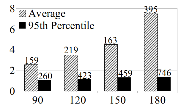
proxy responsiveness ratio

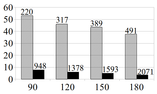
email responsiveness ratio

Figure 13. The relative responsiveness of proxy and email, measured as the response time running on Cilk-F normalized by I-Cilk response time, so higher means I-Cilk is more responsive. Grey bars show the responsiveness calculated using average response time and black bars show that calculated using the response time at $95^{th}$ percentile. The x-axis shows the number of client connections used. The numbers shown on top of the bars are the latency measured in microseconds for I-Cilk.

The high responsiveness is achieved by prioritizing the high-priority threads, sometimes at the expense of the lower priority threads. Figure 14 shows the computation times of threads from different components. For a given application and a given configuration (e.g., proxy with $90$ clients), the bars from left to right show the normalized compute time for threads from higher to lower priority. As the figures show, I-Cilk provides better compute time than Cilk-F for the highest priority threads in the figures (which is the second highest priority for proxy and email). However, the lower priority threads can run slower. This trend can be seen across different server loads, where the compute time ratio for the higher priority threads grows larger as the load gets heavier. This is because the compute time for the higher priority threads on Cilk-F degrades as the server gets more heavily loaded, whereas I-Cilk is able to maintain similar level of quality of service. For the lower-priority threads, compute time on both systems degrades, with I-Cilk degrading more especially when the load gets heavy.

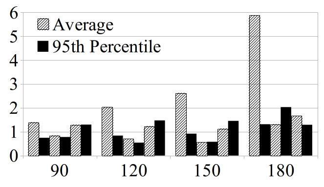
proxy compute time ratio

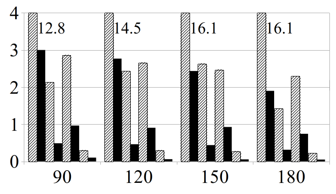
email compute time ratio. Data labels indicate the values of bars that exceed the scale of the graph.

jserver compute time ratio

Figure 14. The relative compute time for proxy, email, and jserver, measured as the compute time running on Cilk-F normalized by that running on I-Cilk, so higher means I-Cilk computes faster. For a given application and a given configuration (e.g., proxy with $90$ clients), the bars from left to right show the compute time ratio for threads from the highest to the lowest priority. The grey bars show the compute time ratio calculated using average compute time and the black bars show that calculated using the compute time at $95^{th}$ percentile. The x-axis shows the number of client connections used for proxy and email, and the server utilization for jserver.

6. Related Work

Cooperative Parallelism

Many languages and systems have been developed for cooperative parallelism over the years. A large number of these, such as Id (Arvind and Gostelow, 1978), Multilisp (Halstead, 1985), NESL (Blelloch et al., 1994) and parallel versions of Haskell (Chakravarty et al., 2007; Keller et al., 2010) and ML (Fluet et al., 2011; Jagannathan et al., 2010; Raghunathan et al., 2016), have focused on functional programming languages, in which the issues of races and deadlock do not arise or are limited.

Some parallel language extensions have, however, targeted popular imperative programming languages such as C (Frigo et al., 1998) and Java (Lea, 2000; Charles et al., 2005; Bocchino et al., 2009; Imam and Sarkar, 2014). Many papers have been devoted over the years to taming races (e.g. (Raman et al., 2012; Feng and Leiserson, 1997; Lee and Schardl, 2015; Utterback et al., 2016; Xu et al., 2018)) and deadlock (e.g. (Voss et al., 2019; Cogumbreiro et al., 2017, 2015; Agarwal et al., 2007)). None of these languages allow the cooperative threads to be prioritized; doing so, as we do in this work, requires reasoning about priority inversions in addition to the problems mentioned above.

Scheduling for Responsiveness

Responsiveness has long been a concern in the systems community, as operating systems must schedule processes and threads, many of which are interactive. A thorough overview of this topic can be found in a text by Silberschatz et al. (2005). In contrast to cooperative parallel systems, OS schedulers deal with relatively small numbers of threads.

Many threading systems for which responsiveness is a concern incorporate some notion of priority. The problem of priority inversion has been noted in systems as early as Mesa (Lampson and Redell, 1980). Babaoğlu et al. (1993) formalized the idea of priority inversions and discussed some techniques by which they could be prevented.

Recent work (Muller et al., 2017, 2018) has introduced thread priorities into a cooperative parallel system and developed type systems for ruling out priority inversions that arise through touching a future. That work, however, targets a purely functional subset of Standard ML, and so future handles can essentially only be passed through calls and returns, leading to a well-behaved DAG structure. In this paper, future handles can additionally be passed through mutable state, leading to much more complicated reasoning about priority inversions.

Cost Semantics

Cost semantics (Rosendahl, 1989; Sands, 1990) are used to reason statically about the resource usage, broadly construed, of programs. Cost semantics for parallel programs (Blelloch and Greiner, 1995, 1996; Spoonhower et al., 2008) typically represent the parallel structure of the program as a DAG. Offline scheduling results bound the time required to execute such a DAG on $P$ processors in terms of the work and span of the DAG. Famous offline scheduling results have shown that a “level-by-level” schedule (Brent, 1974) and any greedy schedule (Eager et al., 1989) are within a factor of two of optimal. Although the full formality of the DAG model is usually reserved for proofs, the metrics of work and span and the scheduling results above are quite useful in practice for analyzing programs by thinking in terms of the parallel structure of the underlying algorithm (e.g., the branching factor and problem size in a divide-and-conquer algorithm). Even in cases where the input is unknown, one can reason asymptotically about work and span, much like asymptotic reasoning in sequential algorithms. Recent work has extended parallel cost semantics to reason about I/O latency (Muller and Acar, 2016) and responsivenesss (Muller et al., 2017, 2018). This paper further extends the state of the art by adding weak edges that allow DAGs to reflect information passed between threads through global state.

Much of the above prior work has drawn a distinction between the cost semantics, which uses a very abstract evaluation model to produce a cost DAG from a program, and a provably-efficient or bounded implementation (Blelloch and Greiner, 1996; Muller et al., 2017, 2018), which counts the steps of an abstract machine. A proof that the abstract machine actually meets the bounds promised by the cost semantics can be quite technical and involved. In this work, we present one dynamic semantics that both counts steps and produces a cost graph. This semantics reflects execution ordering, which is important in our calculus, and simplifies the proof that the steps of the abstract machine are bounded by the cost semantics (this is part of the proof of Theorem 3.8).

7. Conclusion

This paper bridges cooperative and competitive threading models by bringing together a classic threading construct, futures, with priorities and mutable state. To facilitate reasoning about efficiency and responsiveness, the paper extends the traditional graph-based cost models for parallelism to account for priorities and mutable state. The cost model applies only to computations that are free of priority inversions. To guarantee their absence, we present a formal calculus called $\lambda^{4}_{i}$ and a type system that disallows priority inversions. The cost model and the type system both rely on a novel technical device, called weak edges, that represent run-time happens-before dependencies that arise due to communication via mutable shared state. We show that these theoretical results are practical by presenting a reasonably faithful implementation that extends C++ with futures and priorities. This extension offers an expressive substrate for writing interactive parallel programs and is able to enforce the absence of priority inversions if the programmer avoids certain unsafe constructs of C++. Our empirical evaluation shows that the techniques work well in practice.

References

- (1)
- Agarwal et al. (2007) Shivali Agarwal, Rajkishore Barik, Dan Bonachea, Vivek Sarkar, Rudrapatna K. Shyamasundar, and Katherine Yelick. 2007. Deadlock-free Scheduling of X10 Computations with Bounded Resources. In Proceedings of the Nineteenth Annual ACM Symposium on Parallel Algorithms and Architectures (SPAA ’07). ACM, New York, NY, USA, 229–240. https://doi.org/10.1145/1248377.1248416
- Agrawal et al. (2006) Kunal Agrawal, Yuxiong He, Wen Jing Hsu, and Charles E. Leiserson. 2006. Adaptive Task Scheduling with Parallelism Feedback. In Proceedings of the Annual ACM SIGPLAN Symposium on Principles and Practice of Parallel Programming (PPoPP).
- Agrawal et al. (2008) Kunal Agrawal, Yuxiong He, Wen Jing Hsu, and Charles E. Leiserson. 2008. Adaptive scheduling with parallelism feedback. ACM Transactions on Computing Systems 16, 3 (2008), 7:1–7:32.
- Agrawal et al. (2006) Kunal Agrawal, Yuxiong He, and Charles E. Leiserson. 2006. An Empirical Evaluation of Work Stealing with Parallelism Feedback. In Proceedings of the International Conference on Distributed Computing Systems (ICDCS). Lisboa, Portugal.
- Agrawal et al. (2007) Kunal Agrawal, Yuxiong He, and Charles E. Leiserson. 2007. Adaptive work stealing with parallelism feedback. In Proceedings of the 12th ACM SIGPLAN Symposium on Principles and Practice of Parallel Programming (PPoPP ’07). ACM, San Jose, California, USA, 112–120.
- Arora et al. (1998) Nimar S. Arora, Robert D. Blumofe, and C. Greg Plaxton. 1998. Thread scheduling for multiprogrammed multiprocessors. In Proceedings of the tenth annual ACM symposium on Parallel algorithms and architectures (SPAA ’98). ACM Press, 119–129.
- Arora et al. (2001) Nimar S. Arora, Robert D. Blumofe, and C. Greg Plaxton. 2001. Thread Scheduling for Multiprogrammed Multiprocessors. Theory of Computing Systems 34, 2 (2001), 115–144.
- Arvind and Gostelow (1978) Arvind and K. P. Gostelow. 1978. The Id Report: An Asychronous Language and Computing Machine. Technical Report TR-114. Department of Information and Computer Science, University of California, Irvine.
- Babaoğlu et al. (1993) Özalp Babaoğlu, Keith Marzullo, and Fred B. Schneider. 1993. A Formalization of Priority Inversion. Real-Time Systems 5, 4 (1993), 285–303.
- Barik et al. (2009) Rajkishore Barik, Zoran Budimlić, Vincent Cavè, Sanjay Chatterjee, Yi Guo, David Peixotto, Raghavan Raman, Jun Shirako, Sağnak Taşırlar, Yonghong Yan, Yisheng Zhao, and Vivek Sarkar. 2009. The Habanero Multicore Software Research Project. In Proceedings of the 24th ACM SIGPLAN Conference Companion on Object Oriented Programming Systems Languages and Applications (OOPSLA ’09). ACM, Orlando, Florida, USA, 735–736.
- Blake et al. (2010) Geoffrey Blake, Ronald G. Dreslinski, Trevor Mudge, and Krisztián Flautner. 2010. Evolution of Thread-level Parallelism in Desktop Applications. In Proceedings of the 37th Annual International Symposium on Computer Architecture (ISCA ’10). 302–313.
- Blelloch and Greiner (1995) Guy Blelloch and John Greiner. 1995. Parallelism in sequential functional languages. In Proceedings of the 7th International Conference on Functional Programming Languages and Computer Architecture (FPCA ’95). ACM, 226–237.
- Blelloch and Greiner (1996) Guy E. Blelloch and John Greiner. 1996. A provable time and space efficient implementation of NESL. In Proceedings of the 1st ACM SIGPLAN International Conference on Functional Programming. ACM, 213–225.
- Blelloch et al. (1994) Guy E. Blelloch, Jonathan C. Hardwick, Jay Sipelstein, Marco Zagha, and Siddhartha Chatterjee. 1994. Implementation of a Portable Nested Data-Parallel Language. J. Parallel Distrib. Comput. 21, 1 (1994), 4–14.
- Blumofe and Leiserson (1994) Robert D. Blumofe and Charles E. Leiserson. 1994. Scheduling Multithreaded Computations by Work Stealing. 356–368.
- Blumofe and Leiserson (1999) Robert D. Blumofe and Charles E. Leiserson. 1999. Scheduling multithreaded computations by work stealing. J. ACM 46 (Sept. 1999), 720–748. Issue 5.
- Bocchino et al. (2009) Robert L. Bocchino, Jr., Vikram S. Adve, Danny Dig, Sarita V. Adve, Stephen Heumann, Rakesh Komuravelli, Jeffrey Overbey, Patrick Simmons, Hyojin Sung, and Mohsen Vakilian. 2009. A type and effect system for deterministic parallel Java. In Proceedings of the 24th ACM SIGPLAN conference on Object oriented programming systems languages and applications (OOPSLA ’09). 97–116.
- Brent (1974) Richard P. Brent. 1974. The parallel evaluation of general arithmetic expressions. J. ACM 21, 2 (1974), 201–206.
- Cavé et al. (2011) Vincent Cavé, Jisheng Zhao, Jun Shirako, and Vivek Sarkar. 2011. Habanero-Java: the new adventures of old X10. In Proceedings of the 9th International Conference on Principles and Practice of Programming in Java (PPPJ ’11). 51–61.
- Chakravarty et al. (2007) Manuel M. T. Chakravarty, Roman Leshchinskiy, Simon L. Peyton Jones, Gabriele Keller, and Simon Marlow. 2007. Data parallel Haskell: a status report. In Proceedings of the POPL 2007 Workshop on Declarative Aspects of Multicore Programming, DAMP 2007, Nice, France, January 16, 2007. 10–18.
- Charles et al. (2005) Philippe Charles, Christian Grothoff, Vijay Saraswat, Christopher Donawa, Allan Kielstra, Kemal Ebcioglu, Christoph von Praun, and Vivek Sarkar. 2005. X10: an object-oriented approach to non-uniform cluster computing. In Proceedings of the 20th annual ACM SIGPLAN conference on Object-oriented programming, systems, languages, and applications (OOPSLA ’05). ACM, 519–538.
- Cogumbreiro et al. (2015) Tiago Cogumbreiro, Raymond Hu, Francisco Martins, and Nobuko Yoshida. 2015. Dynamic Deadlock Verification for General Barrier Synchronisation. (2015), 150–160. https://doi.org/10.1145/2688500.2688519
- Cogumbreiro et al. (2017) Tiago Cogumbreiro, Rishi Surendran, Francisco Martins, Vivek Sarkar, Vasco T. Vasconcelos, and Max Grossman. 2017. Deadlock Avoidance in Parallel Programs with Futures: Why Parallel Tasks Should Not Wait for Strangers. Proc. ACM Program. Lang. 1, OOPSLA, Article 103 (Oct. 2017), 26 pages. https://doi.org/10.1145/3143359
- Cormen et al. (2009) Thomas H. Cormen, Charles E. Leiserson, Ronald L. Rivest, and Clifford Stein. 2009. Introduction to Algorithms (third ed.). The MIT Press.
- Danaher et al. (2008) John S. Danaher, I-Ting Angelina Lee, and Charles E. Leiserson. 2008. Programming with exceptions in JCilk. Science of Computer Programming 63, 2 (Dec. 2008), 147–171.
- Eager et al. (1989) Derek L. Eager, John Zahorjan, and Edward D. Lazowska. 1989. Speedup versus efficiency in parallel systems. IEEE Transactions on Computing 38, 3 (1989), 408–423.
- Feng and Leiserson (1997) Mingdong Feng and Charles E. Leiserson. 1997. Efficient Detection of Determinacy Races in Cilk Programs. In ACM Symposium on Parallel Algorithms and Architectures. 1–11.
- Flautner et al. (2000) Kristián Flautner, Rich Uhlig, Steve Reinhardt, and Trevor Mudge. 2000. Thread-level Parallelism and Interactive Performance of Desktop Applications. In Proceedings of the Ninth International Conference on Architectural Support for Programming Languages and Operating Systems (ASPLOS IX). 129–138.
- Fluet et al. (2011) Matthew Fluet, Mike Rainey, John Reppy, and Adam Shaw. 2011. Implicitly threaded parallelism in Manticore. Journal of Functional Programming 20, 5-6 (2011), 1–40.
- Fluet et al. (2008) Matthew Fluet, Mike Rainey, John H. Reppy, and Adam Shaw. 2008. Implicitly-threaded parallelism in Manticore. In ICFP. 119–130.
- Frigo et al. (1998) Matteo Frigo, Charles E. Leiserson, and Keith H. Randall. 1998. The Implementation of the Cilk-5 Multithreaded Language. In Proceedings of the ACM SIGPLAN 1998 conference on Programming language design and implementation. 212–223.
- Gao et al. (2014) C. Gao, A. Gutierrez, R. G. Dreslinski, T. Mudge, K. Flautner, and G. Blake. 2014. A study of Thread Level Parallelism on mobile devices. In Performance Analysis of Systems and Software (ISPASS), 2014 IEEE International Symposium on. 126–127.
- Guatto et al. (2018) Adrien Guatto, Sam Westrick, Ram Raghunathan, Umut A. Acar, and Matthew Fluet. 2018. Hierarchical memory management for mutable state. In Proceedings of the 23rd ACM SIGPLAN Symposium on Principles and Practice of Parallel Programming, PPoPP 2018, Vienna, Austria, February 24-28, 2018. 81–93.
- Halstead (1985) Robert H. Halstead. 1985. MULTILISP: a language for concurrent symbolic computation. ACM Transactions on Programming Languages and Systems 7 (1985), 501–538.
- Halstead (1984) Robert H. Halstead, Jr. 1984. Implementation of Multilisp: Lisp on a Multiprocessor. In Proceedings of the 1984 ACM Symposium on LISP and functional programming (LFP ’84). ACM, 9–17.
- Hauser et al. (1993) Carl Hauser, Christian Jacobi, Marvin Theimer, Brent Welch, and Mark Weiser. 1993. Using Threads in Interactive Systems: A Case Study. SIGOPS Oper. Syst. Rev. 27, 5 (Dec. 1993), 94–105.
- Imam and Sarkar (2014) Shams Mahmood Imam and Vivek Sarkar. 2014. Habanero-Java library: a Java 8 framework for multicore programming. In 2014 International Conference on Principles and Practices of Programming on the Java Platform Virtual Machines, Languages and Tools, PPPJ ’14. 75–86.
- Intel (2011) Intel. 2011. Intel Threading Building Blocks. (2011). https://www.threadingbuildingblocks.org/.
- Jagannathan et al. (2010) Suresh Jagannathan, Armand Navabi, KC Sivaramakrishnan, and Lukasz Ziarek. 2010. The Design Rationale for Multi-MLton. In ML ’10: Proceedings of the ACM SIGPLAN Workshop on ML. ACM.
- Keller et al. (2010) Gabriele Keller, Manuel M.T. Chakravarty, Roman Leshchinskiy, Simon Peyton Jones, and Ben Lippmeier. 2010. Regular, shape-polymorphic, parallel arrays in Haskell. In Proceedings of the 15th ACM SIGPLAN international conference on Functional programming (ICFP ’10). 261–272.
- Kuper et al. (2014) Lindsey Kuper, Aaron Todd, Sam Tobin-Hochstadt, and Ryan R. Newton. 2014. Taming the Parallel Effect Zoo: Extensible Deterministic Parallelism with LVish. In Proceedings of the 35th ACM SIGPLAN Conference on Programming Language Design and Implementation (PLDI ’14). ACM, New York, NY, USA, 2–14. https://doi.org/10.1145/2594291.2594312
- Lampson and Redell (1980) Butler W. Lampson and David D. Redell. 1980. Experience with Processes and Monitors in Mesa. Commun. ACM 23, 2 (1980), 105–117.
- Lea (2000) Doug Lea. 2000. A Java fork/join framework. In Proceedings of the ACM 2000 conference on Java Grande (JAVA ’00). 36–43.
- Lee and Schardl (2015) I-Ting Angelina Lee and Tao B. Schardl. 2015. Efficiently Detecting Races in Cilk Programs That Use Reducer Hyperobjects. In Proceedings of the 27th ACM Symposium on Parallelism in Algorithms and Architectures (SPAA ’15). ACM, New York, NY, USA, 111–122. https://doi.org/10.1145/2755573.2755599
- Leijen et al. (2009) Daan Leijen, Wolfram Schulte, and Sebastian Burckhardt. 2009. The design of a task parallel library. In Proceedings of the 24th ACM SIGPLAN conference on Object Oriented Programming Systems Languages and Applications (OOPSLA ’09). 227–242.
- Leiserson (2010) Charles E. Leiserson. 2010. The Cilk++ Concurrency Platform. J. Supercomputing 51, 3 (2010), 244–257.
- Muller and Acar (2016) Stefan K. Muller and Umut A. Acar. 2016. Latency-Hiding Work Stealing: Scheduling Interacting Parallel Computations with Work Stealing. In Proceedings of the 28th ACM Symposium on Parallelism in Algorithms and Architectures, SPAA 2016, Asilomar State Beach/Pacific Grove, CA, USA, July 11-13, 2016. 71–82. https://doi.org/10.1145/2935764.2935793
- Muller et al. (2017) Stefan K. Muller, Umut A. Acar, and Robert Harper. 2017. Responsive Parallel Computation: Bridging Competitive and Cooperative Threading. In Proceedings of the 38th ACM SIGPLAN Conference on Programming Language Design and Implementation (PLDI 2017). ACM, New York, NY, USA, 677–692.
- Muller et al. (2018) Stefan K. Muller, Umut A. Acar, and Robert Harper. 2018. Types and Cost Models for Responsive Parallelism (Draft). In Proceedings of the 14th ACM SIGPLAN International Conference on Functional Programming (ICFP ’18).
- Muller et al. (2019) Stefan K. Muller, Sam Westrick, and Umut A. Acar. 2019. Fairness in Responsive Parallelism. In Proceedings of the 24th ACM SIGPLAN International Conference on Functional Programming (ICFP 2019).
- OpenMP 5.0 (2018) OpenMP 5.0 2018. OpenMP Application Programming Interface, Version 5.0. Accessed in July 2018.
- Raghunathan et al. (2016) Ram Raghunathan, Stefan K. Muller, Umut A. Acar, and Guy Blelloch. 2016. Hierarchical Memory Management for Parallel Programs. In Proceedings of the 21st ACM SIGPLAN International Conference on Functional Programming (ICFP 2016). ACM, New York, NY, USA, 392–406.
- Raman et al. (2012) Raghavan Raman, Jisheng Zhao, Vivek Sarkar, Martin Vechev, and Eran Yahav. 2012. Scalable and Precise Dynamic Datarace Detection for Structured Parallelism. In Proceedings of the 33rd ACM SIGPLAN Conference on Programming Language Design and Implementation (PLDI ’12). ACM, Beijing, China, 531–542.
- Rosendahl (1989) Mads Rosendahl. 1989. Automatic complexity analysis. In FPCA ’89: Functional Programming Languages and Computer Architecture. ACM, 144–156.
- Sands (1990) David Sands. 1990. Complexity Analysis for a Lazy Higher-Order Language. In ESOP ’90: Proceedings of the 3rd European Symposium on Programming. Springer-Verlag, London, UK, 361–376.
- Schardl et al. (2017) Tao B. Schardl, William S. Moses, and Charles E. Leiserson. 2017. Tapir: Embedding Fork-Join Parallelism into LLVM’s Intermediate Representation. In Proceedings of the 22Nd ACM SIGPLAN Symposium on Principles and Practice of Parallel Programming (PPoPP ’17). ACM, Austin, Texas, USA, 249–265. http://doi.acm.org/10.1145/3018743.3018758
- Silberschatz et al. (2005) Abraham Silberschatz, Peter Baer Galvin, and Greg Gagne. 2005. Operating system concepts (7. ed.). Wiley.
- Singer et al. (2019a) Kyle Singer, Yifan Xu, and I-Ting Angelina Lee. 2019a. Proactive Work Stealing for Futures. In Proceedings of the 24th Symposium on Principles and Practice of Parallel Programming (PPoPP ’19). ACM, New York, NY, USA, 257–271. https://doi.org/10.1145/3293883.3295735
- Singer et al. (2019b) Kyle Singer, Yifan Xu, and I-Ting Angelina Lee. 2019b. ProWS - Proactive Work Stealing for Futures. Available at https://github.com/wustl-pctg/ProWS. (2019). Accessed on July 2019.
- Sivaramakrishnan et al. (2014) K. C. Sivaramakrishnan, Lukasz Ziarek, and Suresh Jagannathan. 2014. MultiMLton: A multicore-aware runtime for standard ML. Journal of Functional Programming FirstView (6 2014), 1–62.
- Spoonhower et al. (2008) Daniel Spoonhower, Guy E. Blelloch, Robert Harper, and Phillip B. Gibbons. 2008. Space Profiling for Parallel Functional Programs. In International Conference on Functional Programming.
- Ullman (1975) J.D. Ullman. 1975. NP-complete scheduling problems. J. Comput. System Sci. 10, 3 (1975), 384 – 393.
- Utterback et al. (2016) Robert Utterback, Kunal Agrawal, Jeremy Fineman, and I-Ting Angelina Lee. 2016. Provably Good and Practically Efficient Parallel Race Detection for Fork-Join Programs. In Proceedings of the 28th ACM Symposium on Parallelism in Algorithms and Architectures (SPAA ’16). ACM, Asilomar State Beach, CA, USA, 83–94.
- Voss et al. (2019) Caleb Voss, Tiago Cogumbreiro, and Vivek Sarkar. 2019. Transitive Joins: A Sound and Efficient Online Deadlock-avoidance Policy. In Proceedings of the 24th Symposium on Principles and Practice of Parallel Programming (PPoPP ’19). ACM, New York, NY, USA, 378–390. https://doi.org/10.1145/3293883.3295724
- Xu et al. (2018) Yifan Xu, I-Ting Angelina Lee, and Kunal Agrawal. 2018. Efficient Parallel Determinacy Race Detection for Two-dimensional Dags. In Proceedings of the 23rd ACM SIGPLAN Symposium on Principles and Practice of Parallel Programming (PPoPP ’18). ACM, New York, NY, USA, 368–380. https://doi.org/10.1145/3178487.3178515