Flow heterogeneities in supercooled liquids and glasses under shear

Abstract

Using extensive non-equilibrium molecular dynamics simulations, we investigate a glassforming binary Lennard-Jones mixture under shear. Both supercooled liquids and glasses are considered. Our focus is on the characterization of inhomogeneous flow patterns such as shear bands that appear as a transient response to the external shear. For the supercooled liquids, we analyze the crossover from Newtonian to non-Newtonian behavior with increasing shear rate $\dot{\gamma}$. Above a critical shear rate $\dot{\gamma}_{c}$ where a non-Newtonian response sets in, the transient dynamics are associated with the occurrence of short-lived vertical shear bands, i.e. bands of high mobility that form perpendicular to the flow direction. In the glass states, long-lived horizontal shear bands, i.e. bands of high mobility parallel to the flow direction, are observed in addition to vertical ones. The systems with shear bands are characterized in terms of mobility maps, stress-strain relations, mean-squared displacements, and (local) potential energies. The initial formation of a horizontal shear band provides an efficient stress release, corresponds to a local minimum of the potential energy, and is followed by a slow broadening of the band towards the homogeneously flowing fluid in the steady state. Whether a horizontal or a vertical shear band forms cannot be predicted from the initial undeformed sample. Furthermore, we show that with increasing system size the probability for the occurrence of horizontal shear bands increases.

I Introduction

The structural relaxation in glassforming liquids is associated with a rapidly growing time scale $\tau$. At the glass transition, $\tau$ exceeds the experimentally accessible time scale and the liquid becomes an amorphous solid with an essentially frozen liquid structure glassbook . The slow relaxation processes in the vicinity of the glass transition make the liquid very sensitive to even very small external fields. If a highly viscous liquid is, e.g., sheared with a constant shear rate $\dot{\gamma}$, a new time scale is introduced by $1/\dot{\gamma}$. If this time scale becomes smaller than the time scale for structural relaxation, i.e. $\dot{\gamma}\tau>1$, there is a qualitative change of the response of the liquid to the shear in that it becomes a non-Newtonian liquid chhabra , with the steady-state shear stress, $\sigma_{\rm ss}$, being no longer proportional to the shear rate $\dot{\gamma}$. Structural relaxation processes change qualitatively in the non-Newtonian regime, which is reflected in a decrease of the effective shear viscosity (shear thinning) as well as anisotropies in the structure and dynamics of the sheared liquid berthier2002 ; fuchs2005 ; varnik2006 ; zausch2008 ; zausch2009 .

The transient response of a sheared supercooled liquid, i.e. its behavior before the steady state is reached, also changes qualitatively in the non-Newtonian regime. Here, the stress-strain relation shows a maximum at a strain of the order of 0.1, followed by a stress relaxation towards $\sigma_{\rm ss}$ zausch2008 . A similar behavior is also seen for a glass system in response to an external shear at a constant shear rate. At any finite shear rate, the glass is expected to undergo a transformation from a deformed amorphous solid to a homogeneously flowing fluid in the steady state (provided one waits long enough until the steady state is reached). However, below the glass transition, a Newtonian regime can no longer be seen on experimentally accessible time scales and the extrapolation towards vanishing shear rates, $\dot{\gamma}\to 0$, suggests the approach of a constant value of $\sigma_{\rm ss}$ which can be interpreted as a yield stress. Thus, in this context, the occurrence of a yield stress is a kinetic phenomenon. It is associated with the response of a non-equilibrium glass state and the accessible time scales in experiments (or simulations). One should keep in mind, however, that the “natural response” of an amorphous system to shear is that of a Newtonian fluid in the limit $\dot{\gamma}\to 0$.

The transient behavior of sheared glass can be markedly different from that of a supercooled liquid with respect to the spatial response to the shear field. In supercooled liquids, there are inhomogeneous flow patterns prior to the steady state, albeit these features are usually very weak fuereder2017 . In glasses, however, such inhomogeneities are very pronounced. In particular, there is the possibility for the formation of shear bands, i.e. band-like structures with a higher strain or mobility than in other regions of the system. The occurrence of shear bands is of technological relevance since they can cause the mechanical failure of a glassy material. Shear bands have been observed in experiments of soft matter systems besseling2010 ; divoux2010 ; chikkadi2011 ; divoux2016 and metallic glasses schuh2007 ; maass2015 ; bokeloh2011 ; binkowski2016 as well as in computer simulations of various model glass systems varnik2003 ; bailey2006 ; shi2006 ; shi2007 ; ritter2011 ; sopu2011 ; chaudhuri2012 ; dasgupta2012 ; dasgupta2013 ; albe2013 ; shiva2016_2 ; ozawa2018 ; ozawa2019 ; singh2019 ; parmar2019 ; miyazaki2019 .

Whether or not shear bands form, depends on the degree of annealing of the initial undeformed glass sample and the applied shear rate. This has been recently demonstrated by Ozawa et al. ozawa2018 ; ozawa2019 using an athermal quasistatic shear (aqs) protocol. These authors have also shown that shear bands with an orientation parallel to the flow direction (in the following denoted as horizontal shear bands) are initiated by a very pronounced stress drop in the stress-strain relation. Moreover, in analogy to a first-order phase transition, the stress drop becomes sharper with increasing system size. This has led to the interpretation that the stress drop in the stress-strain relation indicates the presence of the spinodal of a first-order non-equilibrium phase transition ozawa2018 ; procaccia2017 . However, in this picture, the coexisting phases underlying the proposed first-order transition are not identified. As a matter of fact, the inhomogeneous state with shear band is unstable. With further deformation the shear band grows until the system is fully fluidized (see also below). Thus, there is a “transition” from a deformed glass to a homogeneously flowing fluid and the shear-banded structures appear to be transient.

At this point it is interesting to compare the response of glasses and crystals to a deformation. It is tempting to see an analogy of the shear bands in glasses to slip planes in crystals. Slip planes in crystals are located between layers of particles and thereby do not contain any particles. They allow to fully release the stresses in response to a deformation (at least if one considers crystalline systems in the thermodynamic limit) sausset2010 ; nath2018 ; reddy2020 . Unlike a crystal, an amorphous solid can never fully release the stresses in response to a deformation. The stresses that might be localized in a shear band are always carried by particles and, as mentioned above, inhomogeneous systems with shear bands are not stable and transform into a homogeneously flowing fluid state with further deformation. The scenario is completely different in a crystal. Here, at sufficiently small deformation rates, the flow of the crystal can be characterized as a repeated visit of stress-free states nath2018 ; vanmegen1976 .

However, contrary to the first-order transition scenario proposed by Ozawa et al. which requires the existence of overhangs in the stress-strain relation, Barlow et al. barlow have demonstrated using mesoscale constitutive models, that, with increasing age, there can be a gradual change from ductile to brittle-like behaviour. For increased annealing, it has been shown in the framework of mesoscale models moorcroft2013 that there is an increase of the height of the stress overshoot, associated with an increasingly sharper decay towards the steady state stress. In this scenario, when the slope of the latter decay becomes largely negative for more annealed states, a mechanical instability kicks in and shear banding ensues, with the process becoming more catastrophic with larger and larger slopes for more and more aging. In contrast, for the younger ductile materials, where the stress decay is softer, no such flow heterogeneities occur.

In this work, we are aiming at a characterization of inhomogeneous flow patterns in glasses. We use non-equilibrium molecular dynamics (MD) simulations to investigate planar Couette flow in a binary Lennard-Jones system. As a reference, we first consider supercooled liquids for which we analyze the crossover from Newtonian to non-Newtonian behavior with increasing shear rate $\dot{\gamma}$. In the non-Newtonian regime, the stress-strain relations show a stress drop from a maximum stress to the steady-state stress, $\sigma_{\rm ss}$, that decreases with decreasing shear rate and vanishes logarithmically at a critical shear rate $\dot{\gamma}_{c}$. For $\dot{\gamma}<\dot{\gamma}_{c}$, the response of a Newtonian fluid with $\sigma_{\rm ss}\propto\dot{\gamma}$ is seen. After the stress drop, we find the occurrence of vertical shear bands in the transient response of the non-Newtonian fluid. These flow patterns, that form in the direction perpendicular to the flow, are short-lived and can be seen as signatures of the inhomogeneities, observed in the transient response of glasses.

For our study, we consider very low temperature glassy states, where although thermal fluctuations are present, the affine displacements due to the applied deformation dominate over the thermally induced random motion of the particles. This is reflected in a ballistic regime $\propto\dot{\gamma}^{2}t^{2}$ (with $t$ the time) in the mean-squared displacements before the plastic flow sets in. In the considered glasses under shear, we observe in addition to samples with short-lived vertical shear bands, samples with long-lived horizontal shear bands. After their formation, the latter bands exhibit a slow broadening with increasing strain until the system reaches the steady state. Furthermore, it is not imprinted in the initial undeformed glass sample, whether and where horizontal bands form. Instead, we find that their formation is linked to stochasticity; small changes in the protocol such as the use of different initial random numbers for the thermostat can change the flow patterns from vertical to horizontal bands and vice versa. When a system-spanning horizontal shear band is first nucleated after a relatively sharp stress drop, the total potential energy of the system exhibits a minimum with a value which is below that reached in the steady state. So in the case of horizontal shear bands, the transition of the deformed amorphous solid to the homogeneously flowing fluid state takes place via an unstable intermediate state that has, however, a lower potential energy than the final steady state.

The rest of the paper is organized as follows: In the next section, we present the details of the model potential and the MD simulations. Then, in Sec. III, the results for the supercooled liquids and glasses under shear are presented. Finally, we draw conclusions in Sec. IV.

II Model and simulation details

We consider the Kob-Andersen (KA) binary Lennard-Jones mixture kob1994 that has been widely used in many computer simulation studies as a model for a glassforming system. The mixture consists of 80% A particles and 20% B particles. The interaction potential between a particle of type $\alpha$ and a particle of type $\beta$ ($\alpha,\beta=\textrm{A, B}$), separated by a distance $r\leq R_{c}$, is given by

$$u_{\alpha\beta}(r) = \phi_{\alpha\beta}(r)-\phi_{\alpha\beta}(R_{c})-\left(r-R_{c}\right)\left.\frac{d\phi_{\alpha\beta}}{dr}\right|_{r=R_{c}},$$

$$\phi_{\alpha\beta}(r) = 4\epsilon_{\alpha\beta}\left[\left(\sigma_{\alpha\beta}/r\right)^{12}-\left(\sigma_{\alpha\beta}/r\right)^{6}\right]\,.$$ (1)

The values of the interaction parameters are set to $\epsilon_{\textrm{AA}}=1.0$, $\epsilon_{\textrm{AB}}=1.5\epsilon_{\textrm{AA}}$, $\epsilon_{\textrm{BB}}=0.5\epsilon_{\textrm{AA}}$, $\sigma_{\textrm{AA}}=1.0$, $\sigma_{\textrm{AB}}=0.8\sigma_{\textrm{AA}}$, and $\sigma_{\textrm{BB}}=0.88\sigma_{\textrm{AA}}$. In the following, we use $\epsilon_{\textrm{AA}}$ and $\sigma_{\textrm{AA}}$ as the unit for energy and length, respectively. The cutoff radius in Eq. (II) is chosen as $R_{c}=2.5\sigma_{\textrm{AA}}$. As the time unit, we use $\sqrt{{m\sigma_{\textrm{AA}}^{2}}/\epsilon_{\textrm{AA}}}$, where $m$ is the mass of a particle that is considered to be equal for both type of particles, i.e. $m=m_{\textrm{A}}=m_{\textrm{B}}=1.0$. More details about the model can be found in Ref. kob1994 .

We perform the non-equilibrium MD simulation at constant particle number $N$, constant volume $V$, and constant temperature $T$, using the LAMMPS package plimpton1995 . The systems, be they under shear or without shear, are thermostatted via dissipative particle dynamics (DPD) soddemann2003 . The DPD equations of motions are as follows:

$$\dot{\bm{r}}_{i} = {\bm{p}}_{i}/m_{i},$$ (2)

$$\dot{\bm{p}}_{i} = \sum_{j\neq i}\left[{\bm{F}}_{ij}+{\bm{F}}^{\rm D}_{ij}+{\bm{F}}^{\rm R}_{ij}\right],$$ (3)

with ${\bm{r}}_{i}$ the position and ${\bm{p}}_{i}$ the momentum of a particle $i$. Further, ${\bm{F}}_{ij}$ represents the conservative force on a particle pair $i,j$ due to the interparticle interaction, defined by Eq. (II). The dissipative force, ${\bm{F}}^{\rm D}_{ij}$, is given by

$${\bm{F}}^{\rm D}_{ij}=-\zeta\omega^{2}\left(r_{ij}\right)\left(\hat{\bm{r}}_{ij}\cdot{\bm{v}}_{ij}\right)\hat{\bm{r}}_{ij},$$ (4)

with $\zeta$ the friction coefficient, ${\bm{r}}_{ij}$ the distance vector between particles $i$ and $j$, $\hat{\bm{r}}_{ij}$ the unit vector of ${\bm{r}}_{ij}$ , $r_{ij}$ the distance between the two particles, and ${\bm{v}}_{ij}={\bm{v}}_{i}-{\bm{v}}_{j}$ the relative velocity between them.

The value of $\zeta$ is chosen to be equal to $1$. Furthermore, for $\omega\left(r_{ij}\right)$, the following function is used:

$$\omega(r_{ij})=\begin{cases}\sqrt{1-r_{ij}/r_{c}}&\quad if~{}r_{ij}<r_{c},\\ 0&\quad{\rm otherwise}.\end{cases}$$ (5)

The cutoff radius for this function, $r_{c}$, is taken equal to the cutoff radius of the interaction potential, $R_{c}$. In Eq. (3), $F^{\rm R}_{ij}$ represents the random force which is defined as

$$F^{\rm R}_{ij}=\sqrt{2k_{B}T\zeta}\omega(r_{ij})\theta_{ij}\hat{\bm{r}}_{ij}\,.$$ (6)

Here, $\theta_{ij}$ are uniformly-distributed random numbers with zero mean and unit variance. For further details about the DPD thermostat parameters, see Refs. zausch2008 ; zausch2009 . The equation of motion, Eq. (2)-(3), are integrated via the velocity Verlet algorithm using an integration time step $\Delta t=0.005$.

We consider the KA mixture at the two different densities $\rho=1.2$ and $\rho=1.3$ in the supercooled liquid and glass states. For these densities, the mode coupling glass transition temperatures are at $T_{c}=0.435$ and $T_{c}=0.68$, respectively. Note that most recent studies have considered the KA mixture at $\rho=1.2$. However, at this density, one encounters a glass-gas miscibility gap at low temperatures chaudhuri2016_1 ; chaudhuri2016_2 , which is not the case for $\rho=1.3$. Therefore, below we only consider supercooled liquid states at $\rho=1.2$ while at $\rho=1.3$ both supercooled liquids and glasses at very low temperatures are simulated. To prepare the glass samples at $\rho=1.3$, we start with equilibrated samples at $T=0.7$ (in the supercooled regime) and quench it instantaneously to a glass state at the temperature $T=10^{-4}$, followed by aging of the samples over the time $t_{w}=10^{4}$, which would correspond to moderate annealing. For the supercooled liquids at $\rho=1.2$, we have considered cubic samples with linear size $L=30$ and 50. At $\rho=1.3$, cubic samples with linear dimension $L=60$ are chosen. To study finite-size effects, we also report simulations for other system sizes. The details of these simulations can be found below.

We impose a planar Couette flow on the different bulk supercooled liquids and glasses by shearing them along the $xz$-plane in the direction of $x$. The shear is applied via the boundaries using Lees-Edwards boundary conditions lees1972 . The shear rates, $\dot{\gamma}$, considered in this work range from $\dot{\gamma}=10^{-3}$ to $\dot{\gamma}=10^{-7}$ for the supercooled liquid. For the glass state, the shear rate $\dot{\gamma}=10^{-4}$ is chosen. More details about the model and simulation protocol can be found in shiva2016_1 ; shiva2016_2 .

III Results

In the following, we first analyse the transient dynamics of supercooled liquids under shear. We analyse the crossover from Newtonian to non-Newtonian response of the liquid with increasing shear rate. The characterization of non-Newtonian liquids then helps in the understanding of glass states at very low temperature that are considered in the second part of this section. Here, the major issue is the study of transient inhomogeneous flow patterns that form under the application of the shear before the steady state is reached. In particular, different types of shear bands perpendicular and parallel to the flow direction are observed. These flow patterns are analysed in terms of (local) potential energies, shear stresses, and (local) mean-squared displacements (MSDs).

III.1 Supercooled liquids under shear

In a Newtonian fluid, the steady-state shear stress depends linearly on the shear rate, $\sigma_{\rm ss}=\eta\dot{\gamma}$ with $\eta$ the shear viscosity. Deviations from this behavior are expected around a shear rate $\dot{\gamma}_{c}$ when the time scale, associated with this shear rate, is of the order of the time scale $\tau$ for structural relaxation of the unsheared liquid, i.e. $\dot{\gamma}_{c}\tau\approx 1$. As we shall see below, the non-Newtonian response can be inferred from the occurrence of an overshoot in the stress-strain relation.

Shear stress. To compute the shear stress, we use the virial equation, given by

$$\left\langle\sigma_{xz}(t)\right\rangle=\frac{1}{V}\left\langle\sum_{i}\left[m_{i}v_{i,x}v_{i,z}+\sum_{i>j}r_{ij,x}F_{ij,z}\right]\right\rangle\,,$$ (7)

with $V$ the total volume, $m_{i}$ the mass of the $i^{th}$ particle, $v_{i,x}$ and $v_{i,z}$ respectively the $x$ and $z$ components of the velocity of the $i^{th}$ particle, $r_{ij,x}$ the $x$ component of the displacement vector between particles $i$ and $j$, and $F_{ij,z}$ the $z$ component of the force between particles $i$ and $j$. Note that the kinetic terms $\propto m_{i}v_{i,x}v_{i,z}$ are very small and so we have neglected them in our calculation of the shear stress (cf. Ref. zausch2009 ).

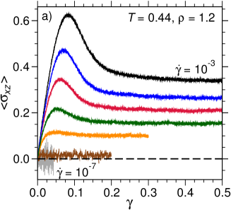
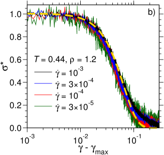
Figure 1: a) Stress-strain relations for the supercooled liquids at $T=0.44$ and $\rho=1.2$ for the shear rates $\dot{\gamma}=10^{-3}$ (black), $3\times 10^{-4}$ (blue), $10^{-4}$ (red), $3\times 10^{-5}$ (green), $10^{-5}$ (orange), $10^{-6}$ (brown), $10^{-7}$ (grey). As a guide to the eye, a dashed horizontal line at zero stress is drawn. b) The reduced stress, $\sigma^{\star}$, as obtained by Eq. (8), for different strain rates in the non-Newtonian regime. The golden dashed line is a fit with a compressed exponential (see text).

In Fig. 1a, we plot the evolution of the stress, $\langle\sigma_{xz}\rangle$, for the supercooled liquid at $T=0.44$ and $\rho=1.2$ as a function of strain, $\gamma=\dot{\gamma}t$, for shear rates $\dot{\gamma}=10^{-3}$, $3\times 10^{-4}$, $10^{-4}$, $3\times 10^{-5}$, $10^{-5}$, $10^{-6}$ and $10^{-7}$. At high shear rates ($\dot{\gamma}=10^{-3},10^{-4}$ and $\dot{\gamma}=10^{-5}$), the stress increases and reaches a maximum at $\sigma_{\rm max}$, from where it relaxes to the steady state stress $\sigma_{\rm ss}$ at large strains. Obviously, the “stress overshoot” at $\sigma_{\rm max}$ decreases with decreasing shear rate and fully disappears at low shear rates (here, this happens at $\dot{\gamma}=10^{-6}$ and $10^{-7}$, see Fig. 1a).

The emergence of the overshoot in the stress-strain relation marks the onset of a non-Newtonian response of the liquid. It is associated with a relaxation of the stress from $\sigma_{\rm max}$ to $\sigma_{\rm ss}$. To analyse this relaxation process, we subtract $\sigma_{\rm ss}$ from the shear stress $\langle\sigma_{xz}\rangle$ and divide this difference by $\sigma_{\rm max}$ to obtain the reduced stress

$$\sigma^{\star}=\frac{\langle\sigma_{xz}\rangle-\sigma_{\rm ss}}{\sigma_{\rm max}}\,.$$ (8)

In Fig. 1b, we plot $\sigma^{\star}$ for different shear rates in the non-Newtonian regime as a function of $\gamma-\gamma_{\rm max}$, where $\gamma_{\rm max}$ corresponds to the strain at the stress $\sigma_{\rm max}$. The curves for the different shear rates fall roughly onto a master curve that can be fitted with the compressed exponential function $f\left(x\right)=\exp\left(-Ax^{B}\right)$, with $x=\gamma-\gamma_{\rm max}$, $A=15.3822$ and $B=1.69862$ (dashed golden line). Note that the fit with the compressed exponential does not provide a perfect description of the data over the whole strain window, but it just gives a rough idea about functional form of the decay of $\sigma$ from $\sigma_{\rm max}$ to $\sigma_{\rm ss}$. The decay of the stress in this manner is intimately related to a superlinear increase of the mean-squared displacement (see Ref. zausch2008 and Fig. 4 below).

Figure 1b also indicates that the strain window over which the stress is released from the stress maximum towards the steady-state stress is of the order of $\Delta\gamma=0.1$. This corresponds to the typical strain required for the breaking of cages around each particle in the supercooled regime above the mode coupling temperature $T_{c}$ zausch2008 . Below, we will see that the decay of $\sigma^{\star}$ for glass states at very low temperatures typically occurs on a smaller strain window.

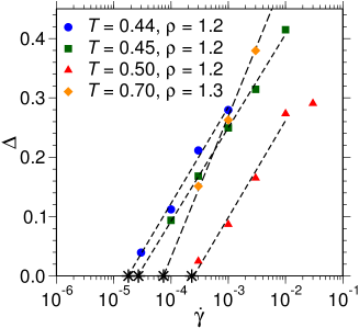
Figure 2: Stress drop $\Delta=\sigma_{\rm max}-\sigma_{\rm ss}$ as a function of shear rate for the indicated densities and temperatures. The dashed lines are fits with the function $f(\dot{\gamma})=A\,{\rm log}(\dot{\gamma}/\dot{\gamma}_{c})$. The stars mark the values of the critical shear rate $\dot{\gamma}_{c}$.

So we have seen that the non-Newtonian regime is characterized by the occurrence of a stress drop $\Delta=\sigma_{\rm max}-\sigma_{\rm ss}$ that decreases with decreasing shear rate and vanishes below a critical shear rate $\dot{\gamma}_{c}$. Thus, this critical shear rate marks the crossover from Newtonian to non-Newtonian behavior. In Fig. 2, the stress drop $\Delta$ is plotted as a function of ${\rm log}(\dot{\gamma})$ for different temperatures at $\rho=1.2$ as well as for $T=0.7$ at $\rho=1.3$. This plot indicates that $\Delta=A\,{\rm log}(\dot{\gamma}/\dot{\gamma}_{c})$, with $A$ and $\dot{\gamma}_{c}$ being fit parameters, holds at sufficiently low shear rates. Here, the critical shear rate $\dot{\gamma}_{c}$ corresponds to the value of $\dot{\gamma}$ at $\Delta=0$. From the fits, we obtain for $\rho=1.2$ the values $\dot{\gamma}_{c}=1.8\times 10^{-5}$, $2.7\times 10^{-5}$, and $2.3\times 10^{-4}$ for $T=0.44$, $T=0.45$, and $T=0.5$, respectively, and for $\rho=1.3$ and $T=0.7$ the value $\dot{\gamma}_{c}=7.4\times 10^{-5}$. In Fig. 2, these values are marked by stars.

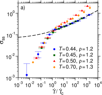
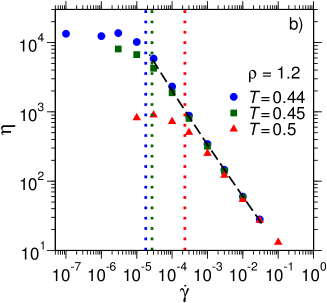
Figure 3: a) The flow curves for the supercooled liquids for the temperatures $T=0.44$, 0.45, and 0.5 at $\rho=1.2$ as well as for the temperature $T=0.7$ at $\rho=1.3$. The dashed line is a fit with a Herschel-Bulkley law (see text). b) The corresponding viscosity $\eta=\sigma_{\rm ss}/\dot{\gamma}$ as a function of $\dot{\gamma}$ for the data at $\rho=1.2$. The black dashed line corresponds to the Herschel-Bulkley law from a), converted to $\eta(\dot{\gamma})$. The dotted vertical lines with different colors mark the values of $\dot{\gamma}_{c}$ corresponding to the different temperatures.

Around the critical shear rate $\dot{\gamma}_{c}$, the flow curve, i.e. the shear rate dependence of the steady-state stress $\sigma_{\rm ss}$, is expected to change from a linear to a non-linear function. Figure 3a shows $\sigma_{\rm ss}$ as a function of $\dot{\gamma}/\dot{\gamma}_{c}$ for $T=0.44$, 0.45, and 0.5 at $\rho=1.2$ as well as for $T=0.7$ at $\rho=1.3$. In the Newtonian regime, the flow curves $\sigma_{\rm ss}(\dot{\gamma}/\dot{\gamma}_{c})$ collapse on top of each other. A non-linear behavior is seen for $\dot{\gamma}/\dot{\gamma}_{c}>1$, i.e. in the non-Newtonian regime. Moreover, in the latter regime, the different curves do not fall onto a master curve which indicates that the characteristic time scale, corresponding to the non-Newtonian regime, is no longer the time scale $\tau$ for structural relaxation ($\alpha$ relaxation) of the unsheared liquid. Now, $\dot{\gamma}>1/\tau$ holds and thus the time scale $1/\dot{\gamma}$ matches relaxation time scales before and during the break-up of the cages around particles that are formed by the other particles. Note that this time regime is often called $\beta$ relaxation regime. At very large shear rates, i.e. $\dot{\gamma}>1$, microscopic time scales of the liquid are probed.

A pronounced $\beta$ relaxation regime (reflected e.g. by a pleateau in the mean-squared displacement, see below) is seen in the quiescent liquid at the temperatures $T=0.44$ and $T=0.45$. For these temperatures, the flow curves can be fitted in the non-Newtonian regime to a Herschel-Bulkley law, $\sigma_{\rm ss}=\sigma_{\rm yield}+A\left(\dot{\gamma}/\dot{\gamma}_{c}\right)^{\alpha}$ with the “yield stress” $\sigma_{\rm yield}=0.0648827$, the amplitude $A=0.0855875$, and the exponent $\alpha=0.295289$ (dashed line in the main plot of Fig. 3a) fn1 . Here, $\sigma_{\rm yield}$ has to be considered as an effective fit parameter. However, for the glass states at temperatures far below $T_{c}$ the yield stress $\sigma_{\rm yield}$ indicates the limiting steady-state stress value, i.e. the stress will not fall below this value with respect to the shear rates that are accessible in the simulation.

The transition to the non-Newtonian regime can be also clearly seen in the behavior of the shear viscosity $\eta=\sigma_{\rm ss}/\dot{\gamma}$, which is shown in Fig. 3b as a function of $\dot{\gamma}$ for the data at $\rho=1.2$. Beyond the Newtonian regime, where $\eta$ is constant, the shear viscosity decreases with increasing shear rate, i.e. we observe shear thinning. We can effectively describe the shear thinning behavior for $\dot{\gamma}>10^{-4}$ by a power law, derived from the Herschel-Bulkley law with which the flow curves at $T=0.44$ and $T=0.45$ are fitted in Fig. 3a. The corresponding fit is shown as a black dashed line in Fig. 3b.

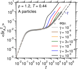
Figure 4: The $z$-component of the MSD of A particles, $\langle\delta r_{{\rm A},z}^{2}\rangle$, as a function of time for the supercooled liquid at $\rho=1.2$ and $T=0.44$. Data, corresponding to the equilibrium ($\dot{\gamma}=0$) and the shear rates $\dot{\gamma}=10^{-3}$, $3\times 10^{-4}$, $10^{-4}$, $3\times 10^{-5}$, $10^{-5}$, $10^{-6}$, and $10^{-7}$, are shown. The dashed line represents a linear function.

One-particle dynamics. The crossover from the Newtonian to the non-Newtonian regime can be also inferred from the one-particle dynamics. An important quantity that characterizes the dynamics of a tagged particle of species $\alpha$ ($\alpha={\rm A,B}$) is the mean-squared displacement (MSD), defined as

$$\langle\delta r_{\alpha}^{2}(t)\rangle=\frac{1}{N_{\alpha}}\sum_{i=1}^{N_{\alpha}}\langle\left|\bm{r}_{i}(t+t_{0})-\bm{r}_{i}(t_{0})\right|^{2}\rangle,$$ (9)

with $\bm{r}_{i}(t)$ the position of particle $i$ of species $\alpha$ at time $t$, $t_{0}$ the time origin, and $N_{\alpha}$ the number of particles of species $\alpha$. The angular brackets correspond to an ensemble average over the different samples.

Figure 4 shows the MSD of A particles in $z$ direction, i.e. in the neutral direction perpendicular to the direction of shear, for the supercooled liquid at $\rho=1.2$, $T=0.44$, and different shear rates. Also included in the figure is the corresponding MSD for the unsheared liquid at equilibrium. This MSD displays the well-known behavior for a supercooled liquid, with a ballistic regime $\propto t^{2}$ at very short times, a diffusive behavior $\propto t$ in the long-time limit, and at intermediate times a subdiffusive plateau-like regime. Note that the MSDs for B particles exhibit a similar behavior. The MSDs corresponding to shear rates in the Newtonian regime coincide with the one at equilibrium, as expected. At higher shear rates ($\dot{\gamma}=10^{-4}$ and $10^{-3}$ in the figure), the MSDs are on top of the one at equilibrium up to the time where the overshoot in the corresponding stress-strain relation occurs. As can be seen in the figure, the stress drop in the stress-strain relation from $\sigma_{\rm max}$ to $\sigma_{\rm ss}$ corresponds to a superlinear increase of the MSD towards a linear diffusive regime when the steady state is reached.

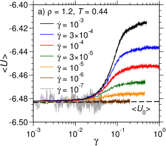
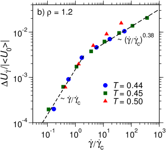
Figure 5: a) The potential energy, $\langle U\rangle$, as a function of strain for the supercooled liquid at $\rho=1.2$ and $T=0.44$. The shear rates are $\dot{\gamma}=10^{-3}$, $3\times 10^{-4}$, $10^{-4}$, $3\times 10^{-5}$, $10^{-5}$, $10^{-6}$, $10^{-7}$. The dashed line marks the potential energy of the undeformed system at $\langle U_{0}\rangle=-6.482$. b) Double-logarithmic plot of the potential energy change $\Delta U_{\dot{\gamma}}/|\langle U_{0}\rangle|$ as a function of $\dot{\gamma}/\dot{\gamma}_{c}$. The dashed lines are fits with power laws, as indicated.

Potential energy. The occurrence of a finite stress in the sheared supercooled liquid is accompanied by a change of the potential energy $\langle U\rangle$. Figure 5a shows $\langle U\rangle$ as a function of strain at $\rho=1.2$ and $T=0.44$ for different shear rates. The transition from the elastic regime to the plastic flow regime is associated with a monotonic increase of $\langle U\rangle$ in the strain window $10^{-}2<\gamma<1.0$ towards a constant value $\langle U_{\rm ss}\rangle(\dot{\gamma})$ in the steady state. To quantify the change of the potential energy from the quiescent state to the steady state, we have computed the difference $\Delta U_{\dot{\gamma}}=\langle U_{\rm ss}\rangle(\dot{\gamma})-\langle U_{0}\rangle$ (with $\langle U_{0}\rangle$ being the potential energy of the unsheared liquid). In Fig. 5b, we plot $\Delta U_{\dot{\gamma}}/|\langle U_{0}\rangle|$ as a function of $\dot{\gamma}/\dot{\gamma}_{c}$. As the figure indicates, $\Delta U_{\dot{\gamma}}$ changes its behavior around $\dot{\gamma}_{c}$, i.e. around $\dot{\gamma}/\dot{\gamma}_{c}=1.0$ there is a crossover from a linear dependence on $\dot{\gamma}/\dot{\gamma}_{c}$ to a power law $\propto(\dot{\gamma}/\dot{\gamma}_{c})^{\alpha}$ with $\alpha<1.0$. For the two lower temperatures, $T=0.44$ and $T=0.45$, the data can be well described by a power law with $\alpha=0.38$. This power law can be seen as the analog to the Herschel-Bulkley law with which we have described the flow curves in the non-Newtonian regime in Fig. 3a.

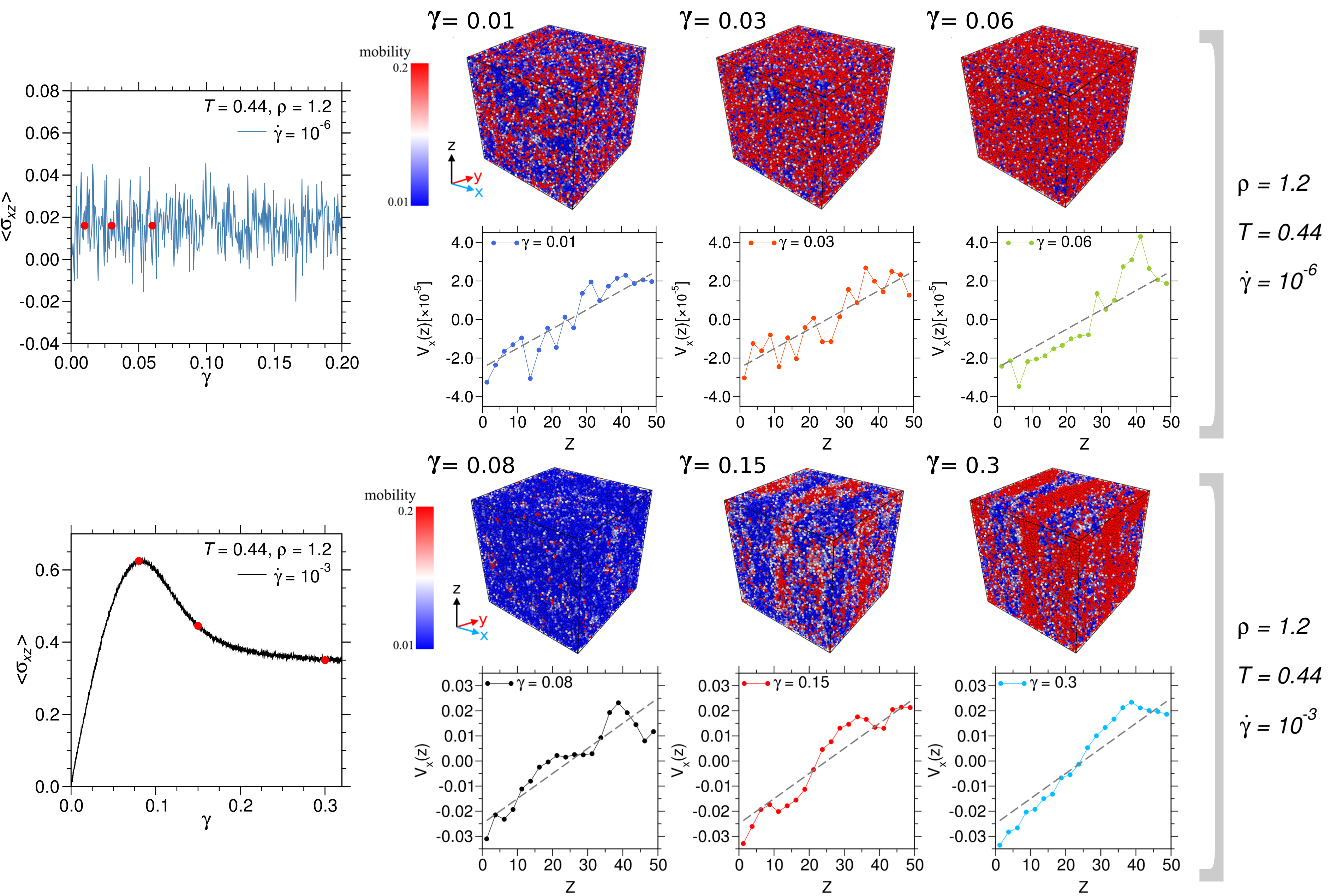
Figure 6: Upper panels: Stress-strain relation, spatial maps of the squared displacement and the corresponding velocity profiles for the supercooled liquid at $\rho=1.2$, $T=0.44$, and $\dot{\gamma}=10^{-6}$ for ${\gamma}=0.01$, 0.03, and 0.06 (these values of $\gamma$ are marked in the plot for $\langle\sigma_{xz}\rangle(\gamma)$ by solid red circles). Lower panels: Same as the upper panel but now at $\dot{\gamma}=10^{-3}$ for ${\gamma}=0.08$, 0.15, and 0.3. For both shear rates, the linear size of the cubic samples is $L=50$.

Flow patterns. Up to now, we have only considered macroscopic properties of the supercooled liquids under shear. As a result, we have characterized the crossover from Newtonian to non-Newtonian behavior for the various quantities as a function of shear rate. Now, we examine the possibility of inhomogeneous flow patterns in the supercooled liquids due to the external shear. To this end, we compute mobility color maps of single-particle, i.e. non-averaged, squared displacements $\delta r_{\alpha,z}^{2}(t)$ at a given strain value $\gamma=\dot{\gamma}t$. Snapshots of such maps for different values of $\gamma$ are displayed in Fig. 6 at $\rho=1.2$ and $T=0.44$ for the shear rates $\dot{\gamma}=10^{-6}$ (Newtonian regime) and $\dot{\gamma}=10^{-3}$ (non-Newtonian regime). Also included in the figure are the corresponding velocity profiles $V_{x}(z)$. The color code is chosen such that blue corresponds to a low and red to a high squared displacement. At the low shear rate, some small spatial heterogeneities can be seen at $\gamma=0.01$, but already at $\gamma=0.06$ the flow is very homogeneous with only small spots of immobile regions. This can be also inferred from the velocity profiles where the deviations from the expected linear behavior (dashed lines) can be refered to thermal noise. Thus, one may conclude from the mobility color maps that there are no pronounced inhomogeneous flow patterns in the Newtonian regime, as expected.

The behavior is qualitatively different at the higher shear rate, $\dot{\gamma}=10^{-3}$, i.e. in the non-Newtonian regime. At a strain of $\gamma=0.08$, most of the particles have a very low squared displacement which indicates the presence of an elastic regime in this case, with an essentially affine deformation of the sample. At the strain $\gamma=0.15$, i.e. slightly after the emergence of the stress overshoot in the stress-strain relation (cf. Fig. 1a), in the direction perpendicular to the shear ($x$ direction), bands of high mobility occur while the rest of the system is still immobile. These vertical shear bands are still present at $\gamma=0.3$. The vertical bands can be, of course, not clearly identified in the corresponding velocity profiles, because they are only sensitive to flow patterns in the direction of shear.

We have identified a critical shear rate $\dot{\gamma}_{c}$ which marks the crossover of the response of the supercooled liquid to the external shear from Newtonian to non-Newtonian behavior. Characteristic features of the non-Newtonian regime are the occurrence of an overshoot in the stress-strain relation, an interim Herschel-Bulkley-like behavior in the flow curve and the potential energy, and a superlinear regime prior to the diffusive steady-state regime in the mean-squared displacement. Furthermore, we observe short-lived vertical shear bands in the non-Newtonian regime that, as we shall see below, also encounter in glasses under shear.

III.2 Glasses under shear

In this section, we analyze glasses under shear. Here, we consider states at the density $\rho=1.3$ and the temperature $T=10^{-4}$. The choice of temperature is such that there are finite but very small thermal fluctuations, but the affine deformation due to the external drive would dominate. Unlike the supercooled liquids, the response of the glass states to the external shear field differs significantly from sample to sample. Therefore, most of the properties that are shown in the following are not obtained by an average over many samples, but we discuss them for individual samples. In particular, even inhomogeneous flow patterns are qualitatively different from sample to sample.

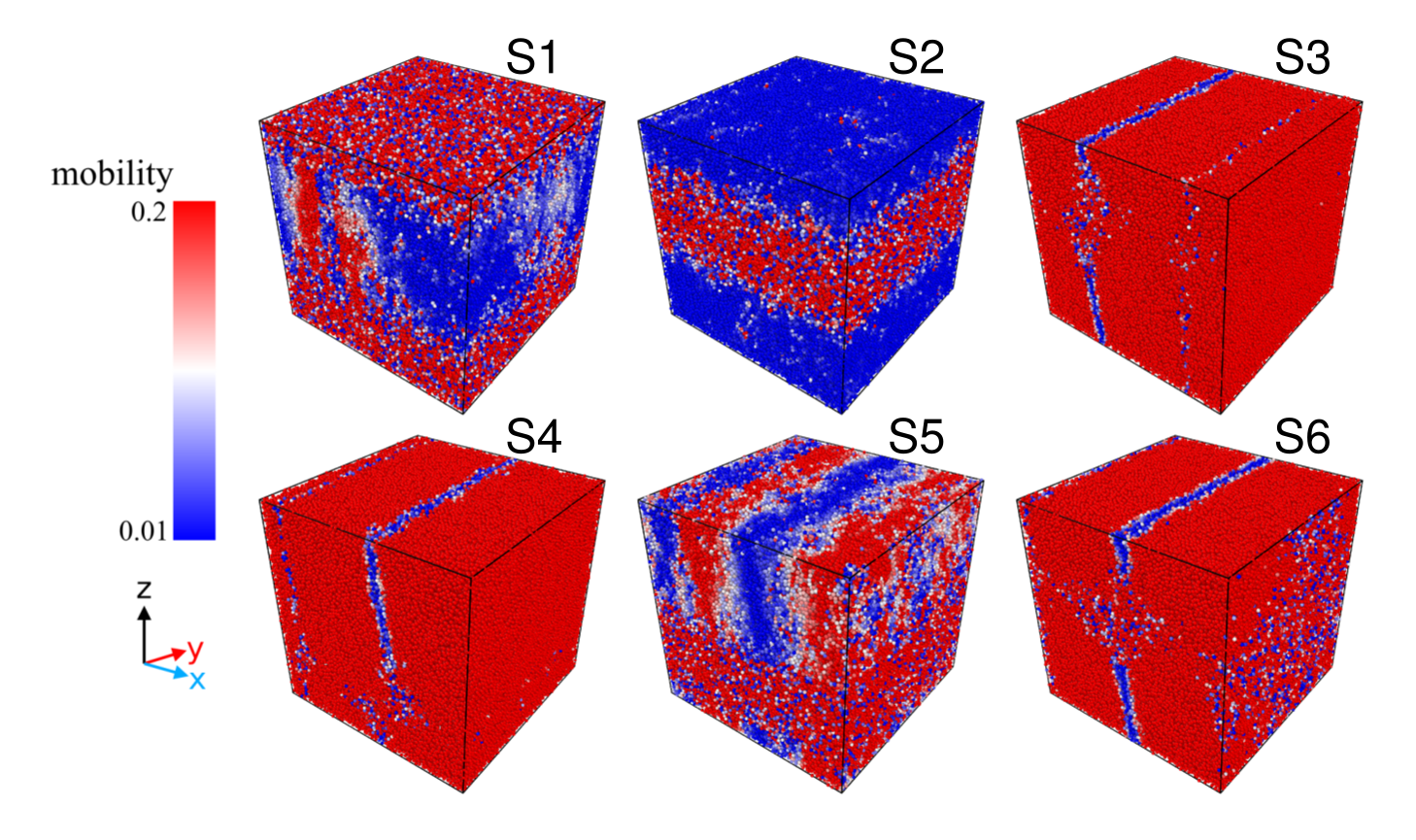
Figure 7: Snapshots of spatial maps of the squared displacement, using different initial glass states, but all with same thermal history, at the strain $\gamma=1.0$. The density, temperature, and shear rate are $\rho=1.3$, $T=10^{-4}$, and $\dot{\gamma}=10^{-4}$, respectively. The linear size of the cubic samples is $L=60$.

Vertical and horizontal shear bands. This is illustrated by the snapshots of spatial maps of the squared displacement at the strain $\gamma=1.0$ in Fig. 7. The corresponding initial configurations before the switch-on of the shear are cubic glass samples with linear dimension $L=60$ at $\rho=1.3$ and $T=10^{-4}$ with a similar thermal history (see above). However, the flow patterns that one can see in the snapshots are obviously different. One can identify two types of shear bands. While the first and second sample has a horizontal shear band, the third, fourth and sixth sample display two vertical shear bands. A mixed situation where both types of shear bands are present can be observed in the fifth sample. We note that at the considered fixed strain of $\gamma=1.0$, the width of the horizontal bands corresponds to about a quarter of the linear dimension of the simulation box ($L=60$). In the cases where two vertical shear bands form after the stress overshoot, these bands have almost merged at $\gamma=1.0$ and the mobility map essentially shows a homogeneously flowing fluid in the steady state.

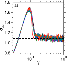
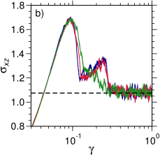
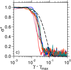
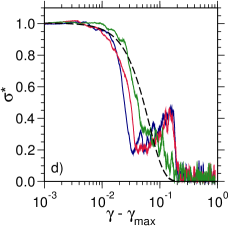
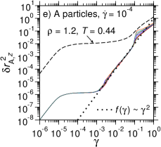
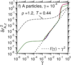
Figure 8: a) and b) Stress-strain relations at $\rho=1.3$, $T=10^{-4}$, and $\dot{\gamma}=10^{-4}$ for different individual cubic samples with linear size $L=60$. The horizontal dashed lines mark the steady-state stress $\sigma_{\rm ss}$. c) and d) Reduced stress $\sigma^{\star}$ as a function of $\gamma-\gamma_{\rm max}$, corresponding to the data shown in a) and b), respectively. The dashed black lines show the compressed exponential function from Fig. 1b. e) and f) The $z$ component of the squared displacement for A particles, $\delta r_{{\rm A},z}^{2}$, as a function of $\gamma$ for different samples, corresponding to those used in a) and b), respectively (in e) and f), the result is averaged over all the A particles in each sample). In e) and f), the dotted lines represent the function $f(\gamma)=a^{2}\gamma^{2}$ with $a=1.0\,\sigma_{\rm AA}$. Also the MSD for the supercooled liquid at $\rho=1.2$, $T=0.44$, and $\dot{\gamma}=10^{-4}$ is included in e) and f).

The stress-strain relations in Figs. 8a and 8b correspond respectively to cases with horizontal and vertical shear bands. Obviously, the stress-strain relations are qualitatively different in both cases. In the case of horizontal shear bands (Fig. 8a), the stress has a maximum at $\gamma_{\rm max}\approx 0.09$, followed by a relatively sharp drop and subsequently a weakly decreasing function towards the steady-state stress. Note that the shear band forms just after the stress drop, as we discuss below. In the case of the vertical shear bands (Fig. 8b), there is a second peak or at least a shoulder after the main stress overshoot. Here, typically two vertical bands are formed after the first overshoot. The fact, that the stress tends to increase again after the occurrence of the first stress drop, indicates that compared to the case of horizontal bands, the vertical ones are rather unstable with a short lifetime and indeed this is what we observe in our simulations. We note that a similar behavior of the stress-strain relation in case of vertical shear bands, i.e. an increase of the stress after the stress overshoot, has been also found in a recent simulation using an aqs protocol kapteijns2019 ; ozawa2019 . While the horizontal shear bands are associated with a larger initial stress drop, in the case of vertical bands, the system evolves much faster towards the steady state. In the case of horizontal bands, the initial stress release is followed by a relatively slow broadening of the shear band (see below).

In Figs. 8c and 8d, the reduced stress $\sigma^{\star}$ as a function of $\gamma-\gamma_{\rm max}$ for the samples corresponding respectively to those in Figs. 8a and 8b are shown. Also included in these plots is the compressed exponential function with which we have fitted the data for the supercooled liquids in Fig. 1b. In the case of the horizontal shear bands, there is a first decay which is clearly faster than that observed for the superooled liquid. However, this fast drop is followed by a slowly decaying tail which is associated with the broadening of the horizontal shear band. Unfortunately, the quality of the data does not allow to analyze the functional behavior of the latter tail. Also in the case of the vertical bands (Fig. 8d), the first stress drop tends to be faster than in the case of the supercooled liquids. Then, there is the occurrence of a second peak or shoulder before quickly approaching the steady state for $\gamma<1.0$.

The $z$ component of the squared displacement for A particles, $\delta r_{{\rm A},z}^{2}$, as a function of $\gamma$ for the samples with horizontal and vertical shear bands are plotted in Fig. 8e and 8f, respectively. In both plots, we have also included for comparison, the corresponding MSD for the supercooled liquid at $\rho=1.2$, $T=0.44$, and $\dot{\gamma}=10^{-4}$, which reveals a completely different behavior of the squared displacement for the glass states at $T=10^{-4}$, as we discuss now. For $\gamma<10^{-3}$, an expected behavior is seen, i.e. after an initial ballistic regime, a plateau at the value $\delta r_{{\rm plat}}^{2}\approx 1.3\times 10^{-6}$ is reached which reflects the strong localization of the particle at the extremely low temperature $T=10^{-4}$ (note that a similar value is obtained for the plateau value of the corresponding unsheared glass state). However, in the interval $10^{-3}<\gamma<10^{-1}$, there is a ballistic regime where $\delta r_{{\rm A},z}^{2}=\gamma^{2}a^{2}=(ut)^{2}$, with $u$ a velocity and $a$ a microscopic length scale of order 1 (in Figs. 8e and 8f we have chosen $a=1.0$). This regime sets in when the condition $\gamma a\approx\sqrt{\delta r_{{\rm plat}}^{2}}$ holds, i.e. at about $\gamma\approx 10^{-3}$. Then, the deformation due to the shear dominates and the small thermal fluctuations are not relevant anymore. However, the strain is not yet sufficient to break the cage around the tagged particle, thus inducing a plastic flow event. This requires still a strain of the order of 0.1. Around the latter strain, plastic flow sets in, which is associated with horizontal shear bands (Fig. 8e) or vertical shear bands (Fig. 8f). As the figures show, for the cases with vertical bands there is a jump in the squared displacements around $\gamma=0.1$ which is much more pronounced than in the case of the horizontal bands.

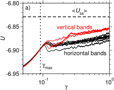
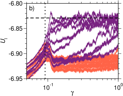
Figure 9: a) Potential energy $U$ as a function of strain $\gamma$ for different samples with horizontal shear band (black solid line) and vertical shear band (red solid line) at $\rho=1.3$, $T=10^{-4}$, and $\dot{\gamma}=10^{-4}$. b) Potential energy, $U_{\rm l}$, for different layers of a sample with horizontal shear band as a function of strain. The linear size of the cubic sample is $L=60$ and it is divided into twenty layers along the $z$ direction, each with a width equal to $3\sigma_{\rm AA}$. The layers that are at $\gamma=1.0$ outside of the shear band are shown by red solid lines while those inside the shear band at $\gamma=1.0$ are represented by the violet solid lines. The horizontal dashed and the vertical dotted lines in both panels mark the average value of the potential energy in the steady state $\langle U_{\rm ss}\rangle=-6.829$ and the strain at the stress overshoot $\gamma_{\rm max}=0.0916$, respectively.

Very pronounced differences between vertical and horizontal shear bands can be also seen in the strain dependence of the potential energy (Fig. 9a). Up to $\gamma\approx 0.1$, the curves for the different samples are on top of each other and, as is the case for the supercooled liquids (cf. Fig. 5a), a monotonic increase of the function $U(\gamma)$ is observed. For $\gamma>0.1$, i.e. when the plastic flow regime sets in, especially in the case of the horizontal shear bands there is an overshoot, followed by a local minimum and a subsequent increase towards the average steady state value of the potential energy vishwas1 ; vishwas2 , marked by the dashed horizontal lines at $\langle U_{\rm ss}\rangle=-6.829$ in the two panels of Fig. 9. So, when the horizontal band is nucleated, the system jumps first to a value of the potential energy which is significantly below the steady state value. This means that the formation of the horizontal band provides a significant release of stress and a lowering of the potential energy. In the case of the vertical bands, the potential energy tends to increase monotonically towards the steady state value. As we have already inferred from the stress-strain relations (cf. Fig. 8), the formation of vertical bands leads to a faster approach of the steady state. However, the formation of a horizontal band is associated with a more efficient stress release and a lower potential energy. Thus, the monitoring of how the potential energy (or pressure) behaves with increasing strain can indicate the spatial orientation of the occurring shear bands.

As we shall see below, the horizontal shear band is transient and broadens as a function of strain. Furthermore, the system with a horizontal shear band corresponds to a state with a local potential energy minimum. This state is very heterogeneous with respect to the spatial distribution of potential energy shi2007 . To analyse this issue, we consider now a sample with horizontal shear band (sample 2 in Fig. 7). We divide the simulation box of this sample into 20 layers along the $z$ direction, each with a width of $3\sigma_{AA}$, and investigate the evolution of the potential energy, $U_{\rm l}$, in each layer. In Fig. 9b, this quantity is shown for each of the 20 layers as a function of $\gamma$. Different colors are assigned to the layers that at $\gamma=1.0$ are inside the shear band region (violet solid lines) and those that are outside the shear band region (red solid lines). Firstly, such spatial resolution allows us to locate the strain value at which the flow heterogeneity sets in, viz. where the divergence of the curves for the different layers occurs, and we note that this happens at a strain value larger than $\gamma_{\rm max}$. Further, the plot also clearly shows that in the shear band the potential energy is already close to the steady-state value, while outside the shear band the system is at significantly lower energy of the order of $-6.92$. The growth of the shear band provides a homogenization of the system and eventually homogeneous flow in the steady state. During this homogenization, the stress slightly decreases towards the steady-state value $\sigma_{\rm ss}$ (cf. Fig. 8a). So the increase of the potential energy from a minimum value after the stress drop to the steady-state value $\sigma_{\rm ss}$, is connected with a further release of the system’s stress.

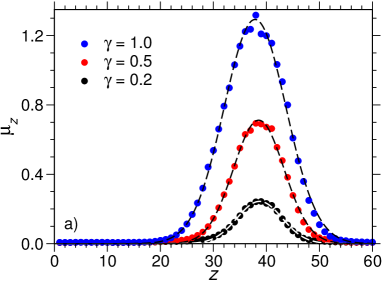
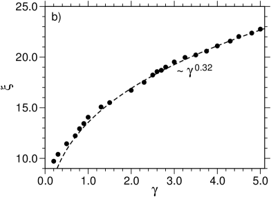
Figure 10: a) Mobility profiles, $\mu_{z}$, as obtained via spatial squared displacement maps of a glass sample with horizontal shear band at $\rho=1.3$, $T=10^{-4}$, and $\dot{\gamma}=10^{-4}$ for $\gamma=0.2$, 0.5, and 1.0. The dashed lines are fits with Gauss functions. b) Width $\xi$ of the shear band as a function of strain (see text). The dashed line represents a power-law fit with exponent $0.32$.

Growth of the shear band. In the case of a sample with a horizontal shear band (sample two in Fig. 7), we examine in Fig. 10 how the shear band grows with increasing strain. To obtain the width of the shear-banded region, we first calculate the mobility profiles along the $z$-direction at different strains. The mobility profiles are defined as the average squared displacement of particles as a function of the distance in $z$-direction. We note that, in our case, the $z$-direction is the gradient direction. In Fig. 10a, we plot the mobility profiles at the three different strains $\gamma=0.2$, 0.5, and 1.0. We fitted the mobility profiles with a Gauss function. The dependence of the width of these Gauss functions, $\xi$, on strain is plotted in Fig. 10b. For $\gamma>1$, the data for $\xi$ can be well described by a power law, $\xi\propto\gamma^{0.32}$, i.e. we find a subdiffusive growth of the horizontal shear band, in agreement with a recent finding by Alix-Williams et al for a Cu-Zr glass model alix2018 .

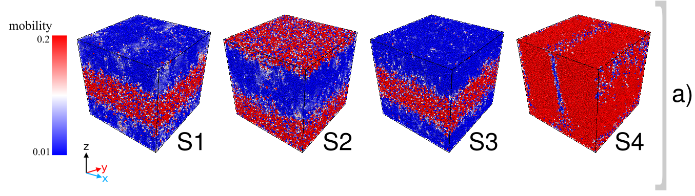
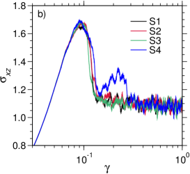
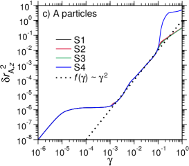
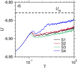
Figure 11: a) Snapshots of mobility color maps for four different glass samples at $\rho=1.3$, $T=10^{-4}$, and $\dot{\gamma}=10^{-4}$ for a strain of $\gamma=1.0$. The initial glass configurations at $\gamma=0$ are identical for all four samples. b) The stress $\sigma_{xz}$, c) the $z$ component of the squared displacement for A particles, $\delta r_{{\rm A},z}^{2}$, and d) the potential energy, $U$, as a function of strain, $\gamma$, for the four sheared glass samples S1 – S4.

Dependence on initial glass states. Now, the question arises whether the type of shear band that is observed after the stress drop around $\gamma=0.1$ is determined by structural heterogeneities in the initial quiescent glass sample. To this end, we choose an initial glass configuration and, starting from this configuration, we perform four different simulations where we shear the system with the same shear rate $\dot{\gamma}=10^{-4}$, but we use in each of these runs a different intitial random seed for the DPD thermostat. So only the random kicks that the particles are facing are different in the four runs. The spatial map of squared displacements at a strain $\gamma=1.0$ is shown in Fig. 11. While the first three samples have horizontal shear bands, the fourth sample forms vertical shear bands (thus, in the latter case, the flow map indicates an almost homogeneously flowing fluid at a strain of $\gamma=1.0$). Furthermore, in the first three samples, the location of the horizontal shear band is different indicating the stochasticity in shear band formation.

The stress-strain relations, the $z$ component of the squared displacement for A particles, and the potential energy for the four samples S1, S2, S3, and S4 are shown in Figs. 11a, 11b, and 11c, respectively. With respect to these quantities, the sample with the vertical shear band (S4) as well as the other three with a horizontal shear band display a similar behavior as found above for the corresponding types of shear bands.

Our findings are consistent with those of Gendelman et al. gendelman2015 who addressed the question whether elementary plastic events, i.e. shear transformation zones (STZs), can be predicted in terms of heterogeneities in the initial unsheared glass sample or are they characterized as events during the mechanical load that depend on the loading protocol. To this end, Gendelman et al. gendelman2015 considered a glass-forming Lennard-Jones mixture in a confined geometry with a circular shape and found that the location of the first plastic event (STZ) depends strongly on the details of the loading protocol. Thus, the location of STZs cannot be simply predicted from the heterogenities of the initial sample before the application of the mechanical load. Our results even suggest a stochastic nature of the occurrence of plastic events and the resulting inhomogeneous flow patterns.

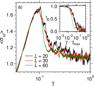
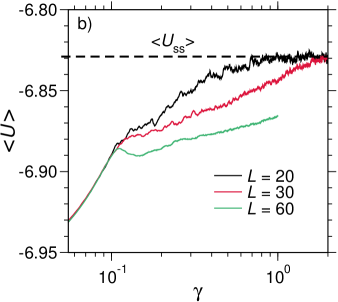
Figure 12: a) Stress-strain relation for three different cubic systems with linear size $L=20$, 30, and 60 in the main panel and the corresponding reduced stress $\sigma^{\star}$ as a function of $\gamma-\gamma_{\rm max}$ in the inset. The inset shows in addition the compressed exponential function from Fig. 1b (dashed black line). b) Potential energy $U$ as a function of strain for the three different systems with $L=20$, 30, and 60. The steady-state value $\langle U_{\rm ss}\rangle=-6.829$ is marked by a horizontal dashed line.

Finite-size effects. Up to now, we have shown results for cubic glass samples with a linear size $L=60$. While in the case of the supercooled liquids under shear we have not observed significant finite-size effects, this is different for the low-temperature glass states. To study finite-size effects, we analyze average properties for systems with linear sizes $L=20$ and $L=30$ in addition to those with $L=60$. The averages were taken over 100, 50, and 10 samples for $L=20$, $L=30$, and $L=60$, respectively. Figure 12a shows the stress-strain relation as well as the decay of $\sigma^{\star}$ as a function of $\gamma-\gamma_{\rm max}$ for the different system sizes. These data suggest that the initial stress drop from $\sigma_{\rm max}$ to $\sigma_{\rm ss}$ is faster for the largest system than for the two smaller systems. This is due to a higher probability for the emergence of horizontal shear bands in large systems. This can be more clearly seen in the strain dependence of the average potential energy, $\langle U\rangle$ (Fig. 12b). The average potential energy for $L=60$ displays the behavior which is associated with the occurrence of horizontal shear bands for $\gamma>0.1$: a drop of $\langle U\rangle$ at $\gamma=0.1$, followed by a shallow minimum and a slow increase towards the steady-state value $\langle U_{\rm ss}\rangle$. For the smaller systems, however, $\langle U\rangle$ essentually exhibits a monotonic and relatively fast increase towards $\langle U_{\rm ss}\rangle$. This is due to the fact that the emergence of horizontal shear bands is less likely for the two smaller systems. We have observed horizontal shear bands in twelve of one hundred samples with linear size $L=20$, in thirteen of fifty samples with $L=30$, and in four of ten samples with $L=60$. Moreover, even when a horizontal shear band forms in the case of small system sizes, the steady state is reached much earlier and at comparable strains the shear banded region covers a larger fraction of the system than for large systems. Thus, at a given strain, the potential energy tends to increase with decreasing system size. However, we have not found significant finite-size effects for the average value of the potential energy in the steady state, $\langle U_{\rm ss}\rangle$.

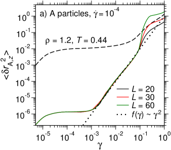
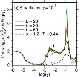
Figure 13: a) The $z$-component of the MSD of A particles, $\langle\delta r_{{\rm A},z}^{2}\rangle$, as a function of strain for the samples with $L=20$, 30, and 60 at $\rho=1.3$, $T=10^{-4}$, and $\dot{\gamma}=10^{-4}$. Also included is the MSD for the supercooled liquid at $\rho=1.2$ and $T=0.44$. The dotted line represents the function $f(\gamma)=a^{2}\gamma^{2}$ (with $a=1.0$). b) The logarithmic derivative, $\Gamma$, corresponding to the MSDs in a).

We have seen that, with increasing the size of the systems with cubic geometry, on average the stress drop in the stress-strain relation becomes sharper. This is also reflected in the behavior of the $z$-component of the MSD of A particles (Fig. 13a). After the ballistic regime $\langle\delta r_{{\rm A},z}^{2}\rangle\propto\gamma^{2}$ in the strain range $10^{-3}<\gamma<10^{-1}$, the MSDs exhibit a jump that becomes more pronounced with increasing system size. This can be also nicely inferred from the exponent parameter $\Gamma$, that is obtained via the logarithmic derivative of the MSD,

$$\Gamma=\frac{d{\rm log}\left(\langle\delta r_{{\rm A},z}^{2}\rangle\right)}{d{\rm log}\langle(\gamma\rangle)}\,.$$ (10)

This quantity is shown Fig. 13b for the different system sizes. Here, we can identify the short-time ballistic regime with $\Gamma=2$ for $\gamma<10^{-6}$, the plateau region with $\gamma\approx 0$ for $10^{-4}<\gamma<10^{-3}$, and the ballistic regime $\propto\gamma^{2}$ with $\Gamma\approx 2$ for $10^{-3}<\gamma<10^{-1}$. In the latter regimes, no finite-size effects are observed. However, for $\gamma\approx 0.1$, there is a peak in $\Gamma({\rm log}\gamma)$ that increases with system size up to a value of $\Gamma\approx 8.0$ for the system with $L=60$. So the stress drop in the stress-strain relation is linked to a jump in the MSD which becomes more pronounced with increasing system size. We note that a similar behavior, albeit much more pronounced, has been recently found by Ozawa et al. ozawa2018 , using an aqs protocol.

IV Summary and conclusions

We have performed non-equilibrium MD simulations of a glassforming binary Lennard-Jones mixture under shear. The shear response of supercooled liquid states has been compared to that of glass states at extremely low, albeit finite, temperature, with the focus on the characterization of yielding and inhomogeneous flow patterns (especially shear bands).

In the supercooled liquid state, we have identified a critical shear rate $\dot{\gamma}_{c}$ that marks the crossover from Newtonian to non-Newtonian response of the liquid to the external shear. For $\dot{\gamma}>\dot{\gamma_{c}}$, i.e. in the non-Newtonian regime, we find inhomogeneous flow patterns in the supercooled liquid in the form of vertical bands. These bands are short-lived and are observed right after the overshoot in the stress-strain relation. The decay of the stress from the maximum stress at the overshoot to the steady-state stress $\sigma_{\rm ss}$ does not seem to depend on shear rate at a given temperature (at least over a large range of shear rates). No finite-size effects are seen in the stress-strain relation, too. The characteristic strain window over which the stress is released is of the order of $\Delta\gamma=0.1$. The potential energy shows a step-like behavior when the system yields, i.e. a monotonic increase again over a strain window of about $\Delta\gamma=0.1$ towards the steady-state value.

In the glass, we have studied the response of glass samples having similar annealing history at a given shear rate, $\dot{\gamma}=10^{-4}$, and temperature, $T=10^{-4}$. For these samples, we observe inhomogeneous flow patterns that differ from sample to sample. In some of them, the plastic flow is associated with relatively short-lived vertical shear bands (i.e. with an orientation perpendicular to the flow direction), while in other samples horizontal bands are seen (i.e. aligned with the flow direction). Also mixed patterns with vertical and horizontal bands are observed. The type of flow pattern that is seen in the transient plastic flow regime is not predetermined by the structure of the initial un-sheared sample. Starting from the same configuration but with different random numbers for the velocity distribution may lead to vertical or to horizontal flow patterns. This indicates the stochasticity of the process. For the sheared glass samples, the behavior of the potential energy is different from that of the supercooled liquids in the non-Newtonian regime. Now, this quantity is not always monotonically increasing towards the steady-state stress. For the cases, where horizontal shear bands occur, the potential energy is higher in the shear band than in the other regions in the system. In the latter regions, it drops to values that are significantly below the final steady-state value. So the system finds a state of lower energy, however this state is not stable in the presence of the applied deformation and so the horizontal shear band broadens as a function of time in a subdiffusive manner. Moreover, in the case of horizontal bands, the stress drop in the stress-strain relation is sharper than that in the supercooled state and it becomes sharper with increasing system size. Furthermore, via a spatial resolution of the system’s potential energy, we show that it is possible to identify the strain value at which horizontal shear-bands emerge, and this occurs beyond the strain where the stress overshoot is observed.

We have seen that there are similarities between the shear response of a supercooled liquid in the non-Newtonian regime and a glass. In both cases, the generic behavior for sufficiently low shear rates is as follows: There is first a strong elastic response to the shear for strains $\gamma<0.1$. This results in a deformed amorphous solid (note that for $\gamma<0.1$ also the supercooled non-Newtonian liquid exhibits solid-like behavior). Then, after a stress release as reflected by a stress drop in the stress-strain relation, the deformed solid eventually transforms into a homogeneously flowing state that can be characterized as an anisotropic non-equilibrium fluid. The latter fluid state is a well-defined stationary state that is obtained at a given shear rate, temperature, and density of the system; in particular, it is independent of the history of the initial unloaded state from which it was obtained via a certain shear protocol. For the sheared glass, the pathways with which the stationary fluid state is reached can completely differ from sample to sample. In the cases with horizontal shear bands one observes a kind of nucleation of the flowing fluid phase that grows slowly towards the homogeneously flowing stationary state.

So the yield point, when identified with the maximum in the stress-strain relation, marks the onset of plastic flow, but it describes a “transition” to a transient state that evolves into a homogeneous fluid state. From this point of view, it is interesting that inhomogeneous states with horizontal shear bands can be stabilized via oscillatory shear. This has been recently shown in two independent simulation studies parmar2019 ; miyazaki2019 . These works have found stationary horizontal shear bands when the maximum strain amplitude in the oscillatory shear is above the critical yield strain, corresponding to the maximum in the stress-strain relation. As a result, an inhomogeneous system is obtained where a fluidized shear-banded region coexists with a glassy region. With respect to potential energy, these states look similar to the ones with horizontal shear bands that we find at a fixed strain (cf. Fig. 9b). However, it is not clear whether the inhomogeneous state that one observes in the oscillatory shear simulation corresponds to a “true” stationary state. If one were able to perform more cycles, the glassy region outside the shear band might further age, as indicated by subdiffusive relaxation processes in Ref. parmar2019 .

While one fixes the window of allowed strains in simulations using an oscillatory shear protocol, one can also perform simulations of glasses subjected to a constant external stress chaudhuri2013 ; cabriolu2019 . As in similar experiments siebenbuerger2012 , one obtains the strain $\gamma$ as a function of time $t$ from such simulations. If the external stress is below the yield stress, there is only creep flow and the strain shows a sublinear increase of the strain as a function of time chaudhuri2013 ; cabriolu2019 ; siebenbuerger2012 . In Ref. chaudhuri2013 , it was shown that this creep flow is associated with the formation of a shear-banded region. Again, this inhomogeneous system with a shear band does not correspond to a stationary state. This is due to the fact that the time scales required to reach a steady state with $\gamma\propto t$ are not accessible by the simulation.

An important issue is the role of long-range strain correlations barrat2011 for the formation of horizontal shear bands. Such correlations are a characteristic feature of elastic media and are also present in supercooled liquids chattoraj2013 ; hassani2018 . The mechanisms of how strain correlations are connected to the formation of inhomogeneous flow patterns is not well understood. It is a subject of forthcoming studies to elucidate this issue.

- (1) K. Binder and W. Kob, Glassy Materials and Disordered Solids: An Introduction to Their Statistical Mechanics, Rev. Ed. (World Scientific, Singapore, 2011).
- (2) R. P. Chhabra and J. F. Richardson, Non-Newtonian Flow and Applied Rheology, 2nd Ed. (Elsevier Butterworth-Heinemann, Oxford, 2008).
- (3) L. Berthier and J.-L. Barrat, J. Chem. Phys. 116, 6228 (2002).
- (4) M. Fuchs and M. Ballauff, J. Chem. Phys. 122, 094707 (2005).
- (5) F. Varnik, J. Chem. Phys. 125, 164514 (2006).
- (6) J. Zausch, J. Horbach, M. Laurati, S. U. Egelhaaf, J. M. Brader, T. Voigtmann, and M. Fuchs, J. Phys.: Condens. Matter 20, 404120 (2008).
- (7) J. Zausch and J. Horbach, EPL 88, 60001 (2009).
- (8) I. Fuereder and P. Ilg, Soft Matter 13, 2192 (2017).
- (9) R. Besseling, L. Isa, P. Ballesta, G. Petekidis, M. E. Cates, and W. C. K. Poon, Phys. Rev. Lett. 105, 268301 (2010).
- (10) T. Divoux, D. Tamarii, C. Barentin, and S. Manneville, Phys. Rev. Lett. 104, 208301 (2010).
- (11) V. Chikkadi, G. Wegdam, D. Bonn, B. Nienhuis, and P. Schall, Phys. Rev. Lett. 107, 198303 (2011).
- (12) T. Divoux, M. A. Fardin, S. Manneville, and S. Lerouge, Ann. Rev. Fluid Mech. 48, 81 (2016).
- (13) C. A. Schuh, T. C. Hufnagel, and U. Ramamurty, Acta Mater. 55, 4067 (2007).
- (14) R. Maaß and J. F. Löffler, Adv. Funct. Mater. 25, 2353 (2015).
- (15) J. Bokeloh, S. V. Divinski, G. Reglitz, and G. Wilde, Phys. Rev. Lett. 107, 235503 (2011).
- (16) I. Binkowski, G. P. Shrivastav, J. Horbach, S. V. Divinski, and G. Wilde, Acta Mater. 109, 330 (2016).
- (17) F. Varnik, L. Bocquet, J.-L. Barrat, and L. Berthier, Phys. Rev. Lett. 90, 095702 (2003).
- (18) N. P. Bailey, J. Schiotz, and K. W. Jacobsen, Phys. Rev. B 73, 064108 (2006).
- (19) Y. Shi and M. L. Falk, Phys. Rev. B 73, 214201 (2006).
- (20) Y. Shi, M. B. Katz, H. Li, and M. L. Falk, Phys. Rev. Lett. 98, 185505 (2007).
- (21) Y. Ritter and K. Albe, Acta Mater. 59, 7082 (2011).
- (22) D. Sopu, Y. Ritter, H. Gleiter, and K. Albe, Phys. Rev. B 83, 100202(R) (2011).
- (23) P. Chaudhuri, L. Berthier, and L. Bocquet, Phys. Rev. E 85, 021503 (2012).
- (24) R. Dasgupta, H. G. E. Hentschel, and I. Procaccia, Phys. Rev. Lett. 109, 255502 (2012).
- (25) R. Dasgupta, O. Gendelman, P. Mishra, I. Procaccia, and C. A. B. Z. Shor, Phys. Rev. E 88, 032401 (2013).
- (26) K. Albe, Y. Ritter, and D. Sopu, Mech. Mater. 67, 94 (2013).
- (27) G. P. Shrivastav, P. Chaudhuri, and J. Horbach, Phys. Rev. E 94, 042605 (2016).
- (28) M. Ozawa, L. Berthier, G. Biroli, A. Rosso, and G. Tarjus, Proc. Natl. Acad. Sci. USA 115, 6656 (2018).
- (29) M. Ozawa, L. Berthier, G. Biroli, and G. Tarjus, preprint arXiv:1912.06021v1.
- (30) M. Singh, M. Ozawa, and L. Berthier, Phys. Rev. Mater. 4, 025603 (2020).
- (31) A. D. S. Parmar, S. Kumar, and S. Sastry, Phys. Rev. X 9, 021018 (2019).
- (32) W.-T. Yeh, M. Ozawa, K. Miyazaki, T. Kawasaki, and L. Berthier, preprint arXiv:1911.12951v1.
- (33) I. Procaccia, C. Rainone, and M. Singh, Phys. Rev. E 96, 032907 (2017).
- (34) F. Sausset, G. Biroli, and J. Kurchan, J. Stat. Phys. 140, 718 (2010).
- (35) P. Nath, S. Ganguly, J. Horbach, P. Sollich, S. Karmakar, and S. Sengupta, Proc. Natl. Acad. Sci. U.S.A. 115, E4322 (2018).
- (36) V. S. Reddy, P. Nath, J. Horbach, P. Sollich, and S. Sengupta, Phys. Rev. Lett. 124, 025503 (2020).
- (37) W. van Megen and I. Snook, Nature 262, 571 (1976).
- (38) H. J. Barlow, J. O. Cochran, and S. M. Fielding, preprint arXiv:1912.07457.
- (39) R. L. Moorcroft and S. M. Fielding, Phys. Rev. Lett. 110, 086001 (2013).
- (40) W. Kob and H. C. Andersen, Phys. Rev. Lett. 73, 1376 (1994).
- (41) S. Plimpton, J. Comput. Phys. 117, 1 (1995).
- (42) T. Soddemann, B. Dünweg, and K. Kremer, Phys. Rev. E 68, 046702 (2003).
- (43) P. Chaudhuri and J. Horbach, Phys. Rev. B 94, 094203 (2016).
- (44) P. Chaudhuri and J. Horbach, J. Stat. Mech. 084005 (2016); doi:10.1088/1742-5468/2016/08/084005.
- (45) A. W. Lees and S. F. Edwards, J. Phys. C: Solid State Phys. 5, 1921 (1972).
- (46) G. P. Shrivastav, P. Chaudhuri, and J. Horbach, J. Rheol. 60, 835 (2016).
- (47) That we give the fit parameter with seven decimal places is just for the purpose of reproducibility of the fit function.
- (48) G. Kapteijns, W. Ji, C. Brito, M. Wyart, and E. Lerner, Phys. Rev. E 99, 012106 (2019).
- (49) V. V. Vasisht, G. Roberts, and E. Del Gado, preprint arXiv:1709.08717.
- (50) V. V. Vasisht and E. Del Gado, preprint arXiv:1908.03943.
- (51) D. D. Alix-Williams and M. L. Falk, Phys. Rev. E 98, 053002 (2018).
- (52) O. Gendelman, P. K. Jaiswal, I. Procaccia, B. S. Gupta, and J. Zylberg, EPL 109, 16002 (2015).
- (53) P. Chaudhuri and J. Horbach, Phys. Rev. E 88, 040301(R) (2013).
- (54) R. Cabriolu, J. Horbach, P. Chaudhuri, and K. Martens, Soft Matter 15, 415 (2019).
- (55) M. Siebenbürger, M. Ballauff, and T. Voigtmann, Phys. Rev. Lett. 108, 255701 (2012).
- (56) J.-L. Barrat and A. Lemaître, in Dynamical Heterogeneities in Glasses, Colloids, and Granular Materials, ed. by L. Berthier, G. Biroli, J.-P. Bouchaud, L. Cipelletti, and W. van Saarloos (Oxford University Press, Oxford, 2011), chap. 8.
- (57) J. Chattoraj and A. Lemaître, Phys. Rev. Lett. 111, 066001 (2013).
- (58) M. Hassani, E. M. Zirdehi, K. Kok, P. Schall, M. Fuchs, and F. Varnik, EPL 124, 18003 (2018).