Extreme mass ratio inspirals with spinning secondary:
a detailed study of equatorial circular motion

Abstract

Extreme mass-ratio inspirals detectable by the future Laser Interferometer Space Antenna provide a unique way to test general relativity and fundamental physics. Motivated by this possibility, here we study in detail the EMRI dynamics in the presence of a spinning secondary, collecting and extending various results that appeared in previous work and also providing useful intermediate steps and new relations for the first time. We present the results of a frequency-domain code that computes gravitational-wave fluxes and the adiabatic orbital evolution for the case of circular, equatorial orbits with (anti)aligned spins. The spin of the secondary starts affecting the gravitational-wave phase at the same post-adiabatic order as the leading-order self-force terms and introduces a detectable dephasing, which can be used to measure it at $5-25\%$ level, depending on individual spins. In a companion paper we discuss the implication of this effect for tests of the Kerr bound.

I Introduction

Extreme mass-ratio inspirals (EMRIs) are among the most interesting gravitational-wave (GW) sources for the future space-based Laser Interferometer Space Antenna (LISA) Audley:2017drz and for evolved concepts thereof Baibhav:2019rsa . An EMRI consists of a stellar-size compact object (henceforth dubbed as secondary) orbiting a supermassive object (henceforth dubbed as primary). The mass ratio of the binary is $q=\mu/M\in(10^{-7}-10^{-4})$ and the secondary makes ${\cal O}(1/q)$ cycles before plunging. This provides a unique opportunity to map the spacetime of the primary and to study radiation-reaction effects that govern the evolution of the orbit.

While parameter estimation still faces challenging open problems Babak:2017tow ; Chua:2019wgs , in principle an EMRI detection with LISA can provide exquisite measurements of the properties of the binary Babak:2017tow . In addition, EMRIs are unique probes of fundamental physics Barack:2018yly ; Barausse:2020rsu . Probing both the conservative and the dissipative sector of the dynamics, they allow for novel tests of gravity Sopuerta:2009iy ; Yunes:2011aa ; Pani:2011xj ; Barausse:2016eii ; Chamberlain:2017fjl ; Cardoso:2018zhm and of the nature of supermassive objects Barack:2006pq ; Pani:2010em ; Babak:2017tow ; Pani:2019cyc ; Datta:2019epe .

With these motivations in mind, in this work we provide a detailed study of the EMRI dynamics in the presence of a spinning secondary. The spin of the secondary starts affecting the gravitational phase to the first order in the post-adiabatic expansion, being thus comparable to the leading-order post-adiabatic self-force effects (which come from the conservative first-order and dissipative second-order in the mass ratio parts of the self-force) Pound:2015tma ; Barack:2018yvs ; Dolan:2013roa ; Burko:2015sqa ; Warburton:2017sxk ; Akcay:2019bvk .

EMRI detection and parameter estimation require accurate first post-adiabatic models of the waveforms Pound:2015tma ; Barack:2018yvs ; Akcay:2019bvk . Therefore, no EMRI inspiral and waveform model is complete without including the spin of the secondary, which motivates several work on this topic.

Earlier work in perturbation theory mostly focused on the effect of the spin on unbound orbits Mino:1995fm ; Saijo:1998mn ; Tominaga:2000cs , and the spin of the secondary was taken to be unrealistically large in order to maximize its effect and compensate for the mass-ratio suppression. One of the first work to consider dissipative spin effects on bound orbits is Ref. Tanaka:1996ht , which estimated post-Newtonian terms for the fluxes by expanding the Teukolsky equation (see also Ref. Nagar:2019wrt for a more recent analysis). A more recent work Dolan:2013roa considered the precession of a gyroscope in Schwarzschild spacetime induced by the conservative self-torque of the particle. The effects of conservative spin-curvature coupling and self-force were studied in Ref. Burko:2003rv ; Burko:2015sqa for circular orbits in Schwarzschild, and later on in Ref. Warburton:2017sxk for generic orbits. The GW fluxes for circular orbits in Schwarzschild and Kerr spacetimes were computed accurately using a time-domain code Harms:2015ixa ; Harms:2016ctx ; Lukes-Gerakopoulos:2017vkj , comparing also some of the most used choices for the supplementary spin conditions discussed below. Recently, Ref. Akcay:2019bvk considered spin dissipative effects with a spinning test particle and derived new flux-balance laws relating the asymptotic fluxes of energy and angular momentum to the adiabatic changes of the orbital parameters, focusing on the case of circular orbits around a Schwarzschild and secondary spin perpendicular to the orbital plane.

An estimate of the conservative contributions on the phase induced by the secondary spin was provided in Ref. Yunes:2010zj using effective-one-body models, while recently Ref. Chen:2019hac calculated the gravitational fluxes including the spin-induced quadrupole in the case of a near extremal Kerr BH. However, to the best of our knowledge, none of the previous work went on to compute explicitly the adiabatic evolution to the leading order and the corresponding spin-correction to the GW phase in a Kerr spacetime, which is crucial to estimate the detectability of the secondary spin. In this work we present a detailed study in this direction for circular, equatorial orbits around a Kerr BH and (anti)aligned spins.

The plan of the paper is as follows. Section II is devoted to an introduction of the motion of a spinning test particle in curved spacetime. In Sec. III the problem is specialized to the case of a primary Kerr metric and, in particular, to circular, equatorial orbits with (anti)aligned spins. The adiabatic approximation used to evolve the orbit and to compute the dephasing is discussed in Sec. IV. Section V is devoted to a brief discussion of the numerical methods used to solve the problem. Results are presented in Sec. VI. Future work is discussed in the conclusion, Sec. VII. In Appendices A and B we provide some details on the Sasaki-Nakamura (SN) equation and on the Teukolsky source term for a spinning particle, collecting and extending various results that appeared in previous work and also providing useful intermediate steps and new relations for the first time. Finally, a comparison with the GW fluxes computed in previous work is presented in Appendix C.

In a companion paper we discuss how measurements of the spin of the secondary can be used to devise model-independent tests of the Kerr bound, i.e. the fact that spinning black holes (BHs) in general relativity cannot spin above a critical value of the angular momentum Piovano:2020ooe .

Throughout this work we use geometric units, $G=c=1$, and define the Riemann tensor as

$${R_{\mu\nu\sigma}}^{\delta}\omega_{\delta}=2\nabla_{[\mu}\nabla_{\nu]}\omega_{\sigma}\ ,$$ (1)

where $\nabla_{\mu}$ is the covariant derivative and $\omega_{\delta}$ an arbitrary 1-form, while the square brackets denote the antisymmetrization. This is the same notation adopted in the package xAct xAct of the software Mathematica, which we used for all the tensor computations. The metric signature is $(-,+,+,+)$.

II Multipole moments and EMRI dynamics

The dynamical evolution of an EMRI can be suitably studied in the framework of perturbation theory, in which a small (secondary) object perturbs the background metric of a larger (primary) BH. If the size of the small body is considerably smaller than the typical scale of the binary, set by the curvature radius of the central object, its stress-energy tensor $T^{\mu\nu}$ allows for a multipolar expansion within the so-called gravitational skeletonization Tulczyjew:1959 ; Dixon:1964NCim ; Dixon:1970I ; Dixon:1970II . Retaining only the first two multipoles is equivalent to consider the secondary as a spinning particle and to neglect tidal interactions, which are encoded in higher multipoles.

For a given worldline $X^{\alpha}(\tau)$, specified by the secondary proper time $\tau$, the multipole moments in general relativity have the following integral representation Kyrian:2007zz

$$\int_{x^{0}=const}T^{\mu\nu}\delta x^{\alpha_{1}}\cdots\delta x^{\alpha_{n}}\sqrt{-g}\,\mathrm{d}^{3}x\ ,$$ (2)

where $\delta x^{\alpha}=x^{\alpha}-X^{\alpha}$ is the deviation from $X^{\alpha}(\tau)$, defined inside the world-tube of the body, and $g=\det(g_{\mu\nu})$ is the determinant of the metric $g_{\mu\nu}$. Hereafter we consider the pole-dipole approximation, by neglecting all moments of the secondary higher than the first two: the linear momentum $p^{\mu}$, and the spin-dipole described by the skew-symmetric tensor $S^{\mu\nu}$:

$$p^{\alpha} =\int_{x^{0}=const}\sqrt{-g}\mathrm{d}^{3}xT^{\alpha 0}\ ,$$ (3)

$$S^{\alpha\beta}(X^{\alpha}) =\int_{x^{0}=const}\sqrt{-g}\mathrm{d}^{3}x(\delta x^{\alpha}T^{\beta 0}-\delta x^{\beta}T^{\alpha 0})\ .$$ (4)

The integrals (3)-(4) are computed choosing a coordinate frame such that $\delta x^{0}=0$, while $\delta x^{i}$ lie inside the integration region. We refer the reader to Refs. Tanaka:1996ht ; Dixon:1964NCim ; Dixon:1978 for a covariant representation of the multipole moments and for a detailed discussion on their properties.

The covariant conservation of the energy-momentum tensor, $\nabla_{\mu}T^{\mu\nu}=0$, leads to the Mathisson- Papapetrou-Dixon (MPD) equations of motion for the spinning test body. These equations were first obtained by Mathisson in linearized theory of gravity Mathisson:1937zz , and then by Papapetrou in full general relativity Papapetrou:1951pa ; Corinaldesi:1951pb . A covariant formulation was obtained by Tulczyjew Tulczyjew:1959 and Dixon Dixon:1964NCim ; Dixon:1970I ; Dixon:1970II , who also included the higher-order multipole moments of the secondary. A modern derivation is given in Ref. Steinhoff:2009tk . The MPD equations of motion read:

$$\frac{\mathrm{d}X^{\mu}}{\mathrm{d}\zeta} =v^{\mu}\ ,$$ (5)

$$\nabla_{\vec{v}}p^{\mu} =-\frac{1}{2}{R^{\mu}}_{\nu\alpha\beta}v^{\nu}S^{\alpha\beta}\ ,$$ (6)

$$\nabla_{\vec{v}}S^{\mu\nu} =2p^{[\mu}v^{\nu]}\ ,$$ (7)

$$\mathfrak{m} \equiv-p_{\mu}v^{\mu}\ ,$$ (8)

where $\nabla_{\vec{v}}\equiv v^{\mu}\nabla_{\mu}$, $v^{\mu}$ is the tangent vector to the representative worldline, and $\zeta$ is an affine parameter that can be different from the proper time $\tau$. Thus, the tangent vector $v^{\mu}$ does not need to be the 4-velocity of a physical observer. The timelike condition $v^{2}\equiv v^{\mu}v_{\mu}<0$ is not a priori guaranteed by the MPD equations, i.e., $v^{2}$ is not necessarily an integral of motion. The mass $\mathfrak{m}$ is the so-called monopole rest-mass, which is related to the energy of the particle as measured in the center of mass frame. The total or dynamical rest mass of the object is given by

$$\mu^{2}=-p^{\sigma}p_{\sigma}\ ,$$ (9)

and represents the mass measured in a reference frame where the spatial components of $p^{\mu}$ vanish. Neither $\mathfrak{m}$ nor $\mu$ are necessarily constants of motion Semerak:1999qc . The spin parameter $S$ is defined as

$$S^{2}\equiv\frac{1}{2}S^{\mu\nu}S_{\mu\nu}\ ,$$ (10)

which is also not a priori conserved. The 4-velocity and the linear momentum are not aligned since

$$p^{\mu}=\frac{1}{v^{2}}(\mathfrak{m}v^{\mu}-v_{\sigma}\nabla_{\vec{v}}S^{\mu\sigma})\ .$$ (11)

The system of MPD equations is undetermined, since there are $18$ dynamical variables $\{X^{\mu},v^{\mu},p^{\mu},S^{\mu\nu}\}$ (note that $S^{\mu\nu}$ is skew-symmetric) and only $15$ equations of motion. One therefore needs to specify $3$ additional constraints to close the system of equations. These constraints are given by choosing a spin-supplementary condition, which fixes the reference worldline with respect to which the moments are computed. We choose as a reference worldline the body’s center of mass. However, in general relativity the center of mass of a spinning body is observer-dependent, thus it is necessary to specify a reference frame by fixing, for example, the spin-supplementary condition covariantly as

$$S^{\mu\nu}V_{\nu}=0\ ,$$ (12)

and by choosing $V^{\nu}$ as the 4-velocity of a physical observer. The representative worldline $X^{\mu}(\zeta)$ identifies then the center of mass measured by an observer with timelike 4-velocity $V^{\nu}$ (for more details see Costa:2011zn ; Costa:2014nta )

Hereafter we choose the Tulczyjew-Dixon condition:

$$S^{\mu\nu}p_{\nu}=0\ ,$$ (13)

which corresponds to $V^{\mu}\equiv p^{\mu}$, i.e. one requires that the center of mass is measured in the frame where $p^{i}=0$. This spin condition fixes a unique worldline, and gives a relation between the 4-velocity $v^{\mu}$ and the linear momentum $p^{\mu}$:

$$v^{\mu}=\frac{\mathfrak{m}}{\mu^{2}}\bigg{(}p^{\mu}+\frac{2S^{\mu\nu}R_{\nu\rho\sigma\!\lambda}p^{\rho}S^{\sigma\!\lambda}}{4\mu^{2}+R_{\alpha\beta\gamma\delta}S^{\alpha\beta}S^{\gamma\delta}}\bigg{)}\ .$$ (14)

Moreover, as a consequence of the Tulczyjew-Dixon spin-supplementary condition, the mass $\mu$ and the spin $S$ become constants of motion, unlike the mass term $\mathfrak{m}$. To fix the latter, we first need to choose an affine parameter $\zeta$ for the MPD equations. One possible choice is setting $\zeta$ equal to the proper time $\tau$, which guarantees that $v^{\mu}v_{\mu}=-1$ throughout the dynamics. Imposing $v^{\mu}v_{\mu}=-1$ automatically fixes $\mathfrak{m}$. Another possibility, first proposed in Ehlers:1977 , (see also Lukes-Gerakopoulos:2017cru ; Witzany:2018ahb ) consists in rescaling $\zeta$ such that

$$p^{\mu}v_{\mu}=-\mu\implies\mu=\mathfrak{m}=const\ ,$$ (15)

which makes $\mathfrak{m}$ constant. In this case however we need to check that $v^{\mu}v_{\mu}<0$ during the orbital evolution. This choice of the affine parameter will be labeled with $\zeta\equiv\lambda$, to differentiate it from the generic affine parameter $\zeta$. It has been numerically shown that, by imposing the same initial conditions, $\lambda$ and $\tau$ are equivalent and lead to the same worldline Lukes-Gerakopoulos:2017cru . In the next sections we will also check that the condition $v^{\mu}v_{\mu}<0$ is always satisfied for all configurations, and that it is equivalent to impose $v^{\mu}v_{\mu}=-1$ and to require that $\mathfrak{m}\in\mathbb{R}$. Finally, the conservation of the mass parameter $\mu$ in the Tulczyjew-Dixon spin-supplementary condition guarantees that the normalization $\mu^{2}=-p^{\mu}p_{\mu}$ holds during the dynamical evolution.

Plugging Eq. (14) into Eq. (7), it is easy to see that

$$\nabla_{\vec{v}}S^{\mu\nu}={\cal O}(q)\,.$$ (16)

Thus, the spin tensor is parallel-transported along the worldline to leading order in the mass ratio.

The freedom in the choice of the spin-supplementary condition reflects the physical requirement that in classical theories particles with intrinsic angular momentum must have a finite size, and that any point of the body can be used to fix the representative worldline. Given $R$ the size of the rotating object, it has been shown that $R\geq S/\mu$ where $S/\mu$ is the Møller radius Moller:1949 . Hence, assuming $R=S/\mu$ and denoting with $\left|{R}_{\mu\nu\rho\sigma}\right|$ the magnitude of the Riemann tensor, the MPD equations are valid as long as the condition $\left|{R}_{\mu\nu\rho\sigma}\right|^{-1}\gg(S/\mu)^{\!2}$ is satisfied, i.e if the size of the spinning secondary is much smaller than the curvature radius of the primary. For a Kerr spacetime, the Kretschmann scalar is $48M^{2}/r^{6}$ on the equatorial plane, so $\left|{R}_{\mu\nu\rho\sigma}\right|\approx M/r^{3}$. Thus, the validity condition of the MPD equations for a Kerr background becomes

$$\left(\frac{r}{M}\right)^{3}\gg\left(\frac{S}{\mu M}\right)^{\!2}\ .$$ (17)

In the following it will be useful to define the dimensionless spin parameter $\sigma$ as

$$\sigma\coloneqq\frac{S}{\mu M}=\chi q\ ,$$ (18)

where $\chi=S/\mu^{2}$ is the reduced spin of the secondary. Regardless of the nature of the secondary, in EMRIs it is expected $|\chi|\ll 1/q$, which implies $|\sigma|\ll 1$. This also shows that Eq. (17) is always satisfied in the EMRI limit.

III Orbital motion

In this section we review the orbital motion of a spinning test particle in the Kerr metric, focusing on the case of circular, equatorial orbits and (anti)aligned spins. Along the way we present some useful intermediate steps and novel relations that, to the best of our knowledge, have not been presented anywhere else.

The background spacetime is described by the Kerr metric in Boyer-Lindquist coordinates,

$$ds^{2}= -dt^{2}+\Sigma(\Delta^{-1}dr^{2}+d\theta^{2})+(r^{2}+a^{2})\sin\theta^{2}d\phi^{2}$$

$$+2Mr/\Sigma(a\sin\theta^{2}-dt)^{2}\ ,$$ (19)

where $\Delta=r^{2}-2Mr+a^{2}$, $\Sigma=r^{2}+a^{2}\cos^{2}\theta$, and $a$ is the spin parameter such that $|a|\leq M$. Without loss of generality, we assume that the specific spin $a$ of the primary is aligned to the $z$-axis, namely $a\geq 0$. The spin $S$ of the secondary is positive (negative) when it is align (antialigned) with the primary spin.

The computations in this section are valid for a generic spin parameter $\sigma$, although later on we will be interested mostly in the case $\sigma\ll 1$ which is relevant for EMRIs.

III.1 Field equations in the tetrad formalism and constants of motion

To describe the orbital motion it is convenient to introduce the following orthonormal tetrad frame (in Boyer-Lindquist coordinates)

$$e^{(0)}_{\mu} =\left(\sqrt{\frac{\Delta}{\Sigma}},0,0,-a\sin^{2}\theta\sqrt{\frac{\Delta}{\Sigma}}\right)\ ,$$ (20)

$$e^{(1)}_{\mu} =\left(0,\sqrt{\frac{\Sigma}{\Delta}},0,0\right)\ ,$$ (21)

$$e^{(2)}_{\mu} =\left(0,0,\sqrt{\Sigma},0\right)\ ,$$ (22)

$$e^{(3)}_{\mu} =\left(-\frac{a}{\sqrt{\Sigma}}\sin\theta,0,0,\frac{r^{2}+a^{2}}{\sqrt{\Sigma}}\sin\theta\right)\ .$$ (23)

We use the notation $e^{(a)}_{\mu}=\big{(}e^{(a)}_{t},\,e^{(a)}_{r},\,e^{(a)}_{\theta},\,e^{(a)}_{\phi}\big{)}$, with the Latin indices for the tetrad components, which are raised/lowered using the metric $\eta^{ab}=\mathrm{diag}(-1,1,1,1)$.

The equations of motion then read

$$\frac{\mathrm{d}}{\mathrm{d}\lambda}p^{(a)}={\omega_{(b)(c)}}^{(a)}v^{(b)}p^{(c)}-\frac{1}{2}{R^{(a)}}_{(b)(c)(d)}v^{(b)}S^{(c)(d)}\ ,$$ (24)

$$\frac{\mathrm{d}}{\mathrm{d}\lambda}S^{(a)(b)}=-2v^{(e)}{\omega_{(e)(c)}}^{{[}(a)}S^{(b){]}(c)}+2p^{{[}(a)}v^{(b){]}}\ ,$$ (25)

where $p^{(a)}=p^{\mu}e^{(a)}_{\mu}$ and so on, whereas ${\omega_{(a)(b)}}^{(c)}\equiv e^{\mu}_{(a)}e^{\nu}_{(b)}\nabla_{\mu}e^{(c)}_{\nu}$ are the Ricci rotation coefficients Mino:1995fm .

The timelike and spacelike Killing vector fields of the Kerr spacetime ($\xi^{\mu}=(1,0,0,0)$ and $\Xi^{\mu}=(0,0,0,1)$, respectively), can be written in the tetrad frame as

$$\xi^{\mu} =\sqrt{\frac{\Delta}{\Sigma}}\,e^{\mu}_{(0)}-\frac{a\sin\theta}{\sqrt{\Sigma}}\,e^{\mu}_{(3)}\ ,$$ (26)

$$\Xi^{\mu} =-a\sin^{2}\theta\sqrt{\frac{\Delta}{\Sigma}}\,e^{\mu}_{(0)}+\frac{(r^{2}+a^{2})\sin\theta}{\sqrt{\Sigma}}\,e^{\mu}_{(3)}\ .$$ (27)

For a generic Killing field $\kappa^{\mu}$ of the background spacetime there exists a first integral of motion

$$C_{\kappa}=p_{\mu}\kappa^{\mu}-\frac{1}{2}\nabla_{\nu}\kappa_{\mu}S^{\mu\nu}\ ,$$ (28)

which is conserved also when higher multipoles are included Ehlers:1977 . The conserved quantities $C_{\xi}\equiv E$ and $C_{\Xi}\equiv J_{z}$ are associated with $\xi^{\mu}$ and $\Xi^{\mu}$, respectively Saijo:1998mn .

It is convenient to introduce the spin vector

$$s^{(a)}\equiv-\frac{1}{2}\epsilon^{(a)(b)(c)(d)}u_{(b)}S_{(c)(d)}\ ,$$ (29)

where $\epsilon_{(a)(b)(c)(d)}$ is the antisymmetric Levi-Civita tensor ($\epsilon_{(0)(1)(2)(3)}=1$) and $u^{(a)}=p^{(a)}/\mu$. The spin tensor can be recast in the following form

$$S^{(a)(b)}\equiv\epsilon^{(a)(b)(c)(d)}u_{(c)}s_{(d)}\ .$$ (30)

III.2 Equations of motion on the equatorial plane

When the orbit is equatorial, and neglecting radiation-reaction effects, it can be shown that if the spin vector is parallel to the $z$-axis, i.e. $s^{\mu}=s^{\theta}\delta^{\mu}_{\theta}$, the spinning particle is constrained on the equatorial plane. In fact, suppose we set $s^{\mu}=s^{\theta}\delta^{\mu}_{\theta}$ as initial condition. By construction, $s^{\mu}p_{\mu}=0$, which implies $p^{\theta}=0$ and $S^{\mu\theta}=0$. Thus, using the equations of motion (7):

$$\nabla_{\vec{v}}S^{\mu\theta}=0\implies p^{\mu}v^{\theta}-p^{\theta}v^{\mu}=0\implies p^{\mu}v^{\theta}=0\ ,$$ (31)

which implies the only nontrivial solution $v^{\theta}=0$. One also needs to prove that $\theta=\pi/2$ is a solution of the equations of motion. From Eq. (6), we have

$$\nabla_{\vec{v}}p^{\theta}=0\implies 0=-\frac{1}{2}{R^{\theta}}_{\nu\alpha\beta}v^{\nu}S^{\alpha\beta}\propto\cos\theta\ ,$$ (32)

which shows that $\theta=\pi/2$ is a solution. If $\theta=\pi/2$ at $\lambda=0$, then the initial condition $s^{\mu}=s^{\theta}\delta^{\mu}_{\theta}$ guarantees that $\theta=\pi/2$ for any value of the evolution parameter $\lambda$. Note that this property does not depend on the spin-supplementary condition.

Hereafter, in order to simplify the notation, we introduce the hatted dimensionless quantities as $\hat{a}=a/M$ and $\hat{r}=r/M$. We also set $s^{(2)}\equiv-S$, such that for $S>0$ (resp. $S<0$) the spin is parallel (resp. antiparallel) to the $z$-axis

Using Eqs. (14),(15) and the normalization $u^{(a)}u_{(a)}=-1$, it is possible to write the velocities $v^{(a)}$ in terms of the normalized momenta $u^{(a)}$

$$v^{(0)}=\frac{1}{N}\bigg{(}1-\frac{\sigma^{2}}{\hat{r}^{3}}\bigg{)}u^{(0)}\ ,$$ (33)

$$v^{(1)}=\frac{1}{N}\bigg{(}1-\frac{\sigma^{2}}{\hat{r}^{3}}\bigg{)}u^{(1)}\ ,$$ (34)

$$v^{(3)}=\frac{1}{N}\bigg{(}1+\frac{2\sigma^{2}}{\hat{r}^{3}}\bigg{)}u^{(3)}\ ,$$ (35)

with $N=1-\frac{\sigma^{2}}{\hat{r}^{3}}\left[1+3\big{(}u^{(3)}\big{)}^{2}\right]$. Likewise, the conserved quantities can be written as Saijo:1998mn

$$\hat{E}=\frac{\sqrt{\Delta}}{\hat{r}}u^{(0)}+\frac{\hat{a}\hat{r}+\sigma}{\hat{r}^{2}}u^{(3)}\ ,$$ (36)

$$\hat{J_{z}}=\frac{\sqrt{\Delta}}{\hat{r}}(\hat{a}+\sigma)u^{(0)}+\left[\frac{\hat{r}^{2}+\hat{a}^{2}}{\hat{r}}+\frac{\hat{a}\sigma}{\hat{r}^{2}}(1+\hat{r})\right]u^{(3)}\ ,$$ (37)

where $\hat{E}=E/\mu$ and $\hat{J}_{z}=J_{z}/(\mu M)$. Since we assumed $a\geq 0$, the orbit is prograde and retrograde for $\hat{J}_{z}>0$ and $\hat{J}_{z}<0$, respectively. At infinity the constant of motion $J_{z}$ can be interpreted as the total angular momentum on the $z$-axis, i.e. the sum $J_{z}\approx L_{z}+S$ of the orbital angular momentum $L_{z}$ and of the spin $S$ of the secondary.

The above relations can be inverted to obtain $u^{(0)}$ and $u^{(3)}$ in terms of $\hat{E}$ and $\hat{J_{z}}$:

$$u^{(0)} =-\frac{\hat{E}\hat{r}^{3}+(\hat{E}\hat{a}-\hat{J_{z}})\sigma+\hat{r}\hat{a}[\hat{J_{z}}-\hat{E}(a+\sigma)]}{\Sigma_{\sigma}\sqrt{\Delta}}\ ,$$ (38)

$$u^{(3)} =\frac{\hat{r}[\hat{J_{z}}-\hat{E}(\hat{a}+\sigma)]}{\Sigma_{\sigma}}\ ,$$ (39)

where

$$\Sigma_{\sigma}=\hat{r}^{2}\left(1-\frac{\sigma^{2}}{\hat{r}^{3}}\right)>0\ ,$$ (40)

which is positive due to the constraint (17). Using Eqs. (38)-(39) and the relations between the velocities $v^{(a)}$ and the normalized momenta $u^{(a)}$ [Eqs. (33)-(35)], we can write the equations of motion in Boyer-Lindquist coordinates as (see also Ref. Saijo:1998mn )

$$\Sigma_{\sigma}\Lambda_{\sigma}\frac{\mathrm{d}\hat{t}}{\mathrm{d}\hat{\lambda}}=\hat{a}\bigg{(}1+\frac{3\sigma^{2}}{\hat{r}\Sigma_{\sigma}}\bigg{)}[\hat{J_{z}}-\hat{E}(\hat{a}+\sigma)]+\frac{\hat{r}^{2}+\hat{a}^{2}}{\Delta}P_{\sigma}\ ,$$ (41)

$$(\Sigma_{\sigma}\Lambda_{\sigma})^{2}\bigg{(}\frac{\mathrm{d}\hat{r}}{\mathrm{d}\hat{\lambda}}\bigg{)}^{\!2}=R^{2}_{\sigma}\ ,$$ (42)

$$\Sigma_{\sigma}\Lambda_{\sigma}\frac{\mathrm{d}\phi}{\mathrm{d}\hat{\lambda}}=\bigg{(}1+\frac{3\sigma^{2}}{\hat{r}\Sigma_{\sigma}}\bigg{)}[\hat{J_{z}}-\hat{E}(\hat{a}+\sigma)]+\frac{\hat{a}}{\Delta}P_{\sigma}\ ,$$ (43)

where

$$\Lambda_{\sigma}=1-\frac{3\sigma^{2}\hat{r}[-(\hat{a}+\sigma)\hat{E}+\hat{J_{z}}]^{2}}{\Sigma^{3}_{\sigma}}\ ,$$ (44)

$$R_{\sigma}=P^{2}_{\sigma}-\Delta\bigg{(}\frac{\Sigma^{2}_{\sigma}}{\hat{r}^{2}}+[-(\hat{a}+\sigma)\hat{E}+\hat{J_{z}}]^{2}\bigg{)}\ ,$$ (45)

$$P_{\sigma}=\bigg{[}(\hat{r}^{2}+\hat{a}^{2})+\frac{\hat{a}\sigma}{\hat{r}}(\hat{r}+1)\bigg{]}\hat{E}-\bigg{[}\hat{a}+\frac{\sigma}{\hat{r}}\bigg{]}\hat{J_{z}}\ ,$$ (46)

and $\frac{1}{\hat{r}^{2}}\Sigma_{\sigma}\Lambda_{\sigma}=N$.

As previously discussed, condition (15) does not necessarily imply $v^{(a)}v_{(a)}<0$ and the latter condition must be checked during the dynamics. The norm of $v^{(a)}$ reads

$$v^{(a)}v_{(a)}=\frac{-\hat{r}^{6}+3\sigma^{2}(u^{(3)})^{2}\big{(}2\hat{r}^{3}+\sigma^{2}\big{)}+2\sigma^{2}\hat{r}^{3}-\sigma^{4}}{(\hat{r}^{3}N)^{2}}\ ,$$

and the constraint $v^{(a)}v_{(a)}<0$ leads to

$$\Lambda_{\sigma}>\frac{\hat{r}^{3}+2\sigma^{2}}{2\hat{r}^{3}+\sigma^{2}}\ .$$ (47)

Equation (47) shows that $\Lambda_{\sigma}$ must be positive definite, which implies $N>0$. Moreover, for realistic values of $\sigma$ (recall that $|\sigma|\ll 1$ when $|\chi|\ll 1/q$, see Eq. (18)) the constraint (47) reduces to

$$\Lambda_{\sigma}\gtrsim\frac{1}{2}\quad\text{ for}\quad\sigma\ll 1$$ (48)

and, since $\hat{E}$ and $\hat{J}_{z}$ are usually ${\cal O}(1)$ during the dynamics, $\Lambda_{\sigma}\approx 1\text{ for }\sigma\ll 1$. Thus Eq. (47) is always satisfied for bound equatorial EMRIs. Finally, we note that choosing the proper time of the object as evolution parameter, the condition $v^{(a)}v_{(a)}=-1$ fixes the kinematical mass $\mathfrak{m}$ as

$$\mathfrak{m}(\hat{r})=\frac{\hat{r}^{3}N}{\sqrt{\hat{r}^{6}-3\sigma^{2}(u^{(3)})^{2}\big{(}2\hat{r}^{3}+\sigma^{2}\big{)}-2\sigma^{2}\hat{r}^{3}+\sigma^{4}}}\ .$$ (49)

Imposing that $\mathfrak{m}(\hat{r})$ is a real number gives again the constraint (47).

III.3 Effective potential, ISCO, and orbital frequency

For circular orbits, there are two additional constraints on the motion: one enforces zero radial velocity, the other requires zero radial acceleration. The condition $v^{r}=0$ implies $v^{(1)}=0$ and, together with Eq. (34) yields $p^{(1)}=0$, whereas zero radial acceleration requires $\frac{\mathrm{d}}{\mathrm{d}\lambda}p^{(1)}=0$. Imposing these constraints is equivalent to ask the orbital radius to be the local minimum of an effective potential. For a spinning particle moving on the equatorial plane of a Kerr BH, the effective potential depends on the spin-supplementary condition (see Refs. Harms:2016ctx ; Lukes-Gerakopoulos:2017vkj for the form of the effective potentials for some common choices of the spin-supplementary conditions). Following Ref. Jefremov:2015gza we use

$$V_{\sigma}(\hat{r})=\frac{1}{\hat{r}^{4}}(\alpha_{\sigma}\hat{E}^{2}-2\beta_{\sigma}\hat{E}+\gamma_{\sigma})\ ,$$ (50)

where

$$\alpha_{\sigma} =\left[\hat{r}^{2}+\hat{a}^{2}+\frac{\hat{a}\sigma(\hat{r}+1)}{\hat{r}}\right]^{2}-\Delta(\hat{a}+\sigma)^{2}\ ,$$ (51)

$$\beta_{\sigma} =\bigg{[}\bigg{(}\hat{a}+\frac{\sigma}{\hat{r}}\bigg{)}\bigg{(}\hat{r}^{2}+\hat{a}^{2}+\frac{\hat{a}\sigma(\hat{r}+1)}{\hat{r}}\bigg{)}-\Delta(\hat{a}+\sigma)\bigg{]}\hat{J}_{z}\ ,$$ (52)

$$\gamma_{\sigma} =\bigg{(}\hat{a}+\frac{\sigma}{\hat{r}}\bigg{)}^{\!\!2}\hat{J}_{z}^{2}-\Delta\bigg{[}\hat{r}^{2}\bigg{(}1-\frac{\sigma^{2}}{\hat{r}^{3}}\bigg{)}^{\!\!2}+\hat{J}_{z}^{2}\bigg{]}\ .$$ (53)

The effective potential reduces to the standard one for a nonspinning particle in Kerr when $\sigma=0$. The condition for a circular orbit with radius $\hat{r}_{0}$ translates to

$$V_{\sigma}(\hat{r}_{0})=0 \quad\quad\ ,\left.\frac{\mathrm{d}V_{\sigma}}{\mathrm{d}\hat{r}}\right\rvert_{\hat{r}=\hat{r}_{0}}=0\ ,$$

and stability of such orbits against radial perturbations requires $\left.\frac{\mathrm{d}^{2}V_{\sigma}}{\mathrm{d}\hat{r}^{2}}\right\rvert_{\hat{r}=\hat{r}_{0}}<0$, although the orbit might still be unstable under perturbation in the $\theta$ direction Suzuki:1997by . The innermost stable circular orbit (ISCO) is obtained by imposing $\left.\frac{\mathrm{d}^{2}V_{\sigma}}{\mathrm{d}\hat{r}^{2}}\right\rvert_{\hat{r}=\hat{r}_{0}}=0$.

In order to compute the GW fluxes, we also need the orbital frequency of a circular equatorial orbit as measured by an observer located at infinity,

$$\widehat{\Omega}=M\Omega=\frac{\mathrm{d}\phi}{\mathrm{d}\hat{t}}=\frac{\hat{a}v^{(0)}+\sqrt{\Delta}v^{(3)}}{(\hat{r}^{2}+\hat{a}^{2})v^{(0)}+\hat{a}\sqrt{\Delta}v^{(3)}}\ .$$

In terms of the momenta $\hat{\Omega}$ is given by

$$\widehat{\Omega}=\frac{\hat{a}(\hat{r}^{3}-\sigma^{2})u^{(0)}+\sqrt{\Delta}(\hat{r}^{3}+2\sigma^{2})u^{(3)}}{(\hat{r}^{2}+\hat{a}^{2})(\hat{r}^{3}-\sigma^{2})u^{(0)}+\hat{a}\sqrt{\Delta}(\hat{r}^{3}+2\sigma^{2})u^{(3)}}\ ,$$ (54)

where $u^{(0)}$ and $u^{(3)}$ are given in terms of $\hat{r}$ by solving $\frac{\mathrm{d}}{\mathrm{d}\lambda}p^{(1)}=0$:

$$u^{(0)}=\frac{1}{\sqrt{1-U_{\mp}^{2}}}\ , \qquad u^{(3)}=\frac{U_{\mp}}{\sqrt{1-U_{\mp}^{2}}}\ ,$$ (55)

where Tanaka:1996ht

$$U_{\mp}=\frac{u^{(3)}}{u^{(0)}}=-\frac{2\hat{a}\hat{r}^{3}+3\sigma\hat{r}^{2}+\hat{a}\sigma^{2}\mp{\cal D}}{2\sqrt{\Delta}(\hat{r}^{3}+2\sigma^{2})}\ ,$$ (56)

with

$${\cal D}=\sqrt{4\hat{r}^{7}+12\hat{a}\sigma\hat{r}^{5}+13\sigma^{2}\hat{r}^{4}+6\hat{a}\sigma^{3}\hat{r}^{2}-8\sigma^{4}\hat{r}+9\hat{a}^{2}\sigma^{4}}\ ,$$ (57)

and the $\mp$ sign corresponding to co-rotating and counter-rotating orbits, respectively. Note that the argument of the square root is not positive definitive for generic values of $\sigma$. Nevertheless, for $\sigma\ll 1$, it is easy to see that Eq. (56) is always real. Using Eq. (55), the orbital frequency $\widehat{\Omega}$ can be recast as

$$\widehat{\Omega}=\frac{(2\hat{a}+3\sigma)\hat{r}^{3}+3(2\hat{a}^{2}\sigma+\hat{a}\sigma^{2})\hat{r}+4\hat{a}\sigma^{2}\mp\hat{r}{\cal D}}{2(\hat{a}^{2}+3\hat{a}\sigma+\sigma^{2})\hat{r}^{3}+6\sigma(\hat{a}+\sigma)\hat{a}^{2}\hat{r}+4\hat{a}^{2}\sigma^{2}-2\hat{r}^{6}}\ .$$ (58)

This formula agrees with the one shown in Ref. Harms:2015ixa . Plugging Eq. (55) into Eqs. (36)-(37) finally yields the first integrals $\hat{E}$ and $\hat{J}_{z}$ for a spinning object in circular equatorial orbit in the Kerr spacetime:

$$\hat{E} =\frac{\hat{r}\sqrt{\Delta}+(\hat{a}\hat{r}+\sigma)U_{\mp}}{\hat{r}^{2}\sqrt{1-U_{\mp}^{2}}}\ ,$$ (59)

$$\hat{J}_{z} =\frac{\hat{r}\sqrt{\Delta}(\hat{a}+\sigma)+[\hat{r}^{3}+\hat{r}\hat{a}(\hat{a}+\sigma)+\hat{a}\sigma]U_{\mp}}{\hat{r}^{2}\sqrt{1-U_{\mp}^{2}}}\ .$$ (60)

The minus and plus sign in Eq. (58)-(60) correspond to prograde and retrograde orbits, respectively. Expressions (59) and (60) will be useful when studying the adiabatic evolution of the orbit.

Furthermore, the above quantities can be used to derive analytical expressions for the ISCO location and frequency to ${\cal O}(\sigma)$ (see also Ref. Jefremov:2015gza ). The orbital frequency can be written as

$$\widehat{\Omega}(\hat{r})=\widehat{\Omega}^{0}(\hat{r})+\sigma\delta\widehat{\Omega}(\hat{r})+{\cal O}(\sigma^{2})\ ,$$ (61)

where $\widehat{\Omega}^{0}(\hat{r})=1/(\hat{a}\pm\hat{r}^{3/2})$ is the orbital frequency of a nonspinning particle around Kerr, and

$$\delta\widehat{\Omega}(\hat{r})=-\frac{3}{2}\frac{\sqrt{\hat{r}}\mp\hat{a}}{\sqrt{\hat{r}}(\hat{r}^{3/2}\pm a)^{2}}\,.$$ (62)

The ISCO location can be expanded in the same way and its leading-order spin correction reads

$$\delta\hat{r}_{\rm ISCO}=\frac{4\hat{a}}{\hat{r}_{\rm ISCO}^{0}}\mp\frac{4}{\sqrt{\hat{r}_{\rm ISCO}^{0}}}\,,$$ (63)

where $\hat{r}_{\rm ISCO}^{0}$ is the (normalized) ISCO location of the Kerr metric for a nonspinning secondary, which is solution to $\hat{r}^{2}-6\hat{r}+8\hat{a}\hat{r}^{1/2}-3\hat{a}^{2}=0$ (its analytical expression as a function of $\hat{a}$ can be found in Ref. 1972ApJ…178..347B ). Using the above results, the leading-order spin correction to the ISCO orbital frequency is

$$\delta\widehat{\Omega}_{\rm ISCO}=\frac{9}{2}\left(\frac{\sqrt{\hat{r}_{\rm ISCO}^{0}}\mp\hat{a}}{\sqrt{\hat{r}_{\rm ISCO}^{0}}\left((\hat{r}_{\rm ISCO}^{0})^{3/2}\pm\hat{a}\right)^{2}}\right)\,.$$ (64)

This quantity is shown in Fig. 1 as a function of $\hat{a}$ for prograde orbits (upper sign Eq. (64)). Note that $\delta\widehat{\Omega}_{\rm ISCO}>0$ for any $\hat{a}$ (being zero in the extremal case), i.e., if the spin of the secondary is aligned to that of the primary the orbital frequency at the ISCO is higher.

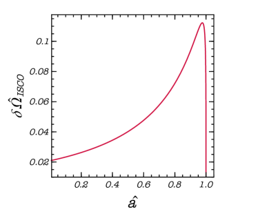
Figure 1: Spin correction to the orbital frequency at the ISCO as a function of $\hat{a}$ for prograde orbits (upper sign Eq. (64))

IV Radiation-reaction effects and balance laws

We study radiation-reaction effects within the adiabatic approximation, assuming that the emission timescale is much longer than orbital period, namely

$$\frac{2\pi}{\widehat{\Omega}}\ll\hat{r}\left|\frac{\mathrm{d}\hat{r}}{\mathrm{d}\hat{t}}\right|^{-1}\,.$$ (65)

In this approximation, changes to the mass terms $\mu$ and $M$ and to the spin $\hat{a}$ are smaller than the leading-order dissipative terms Hinderer:2008dm . The change to the primary mass and spin due to GW absorption at the horizon formally enter at the next-to-leading order, although with a small coefficient Hughes:2018qxz .

Thus, for a nonspinning object on an equatorial orbit around a Kerr BH

$$\frac{\mathrm{d}E}{\mathrm{d}t}=\Omega\frac{\mathrm{d}L_{z}}{\mathrm{d}t}\,.$$ (66)

In the adiabatic approximation, the following balance equations hold:

$$\left(\frac{\mathrm{d}E}{\mathrm{d}t}\right)_{\!\!\text{GW}}=-\left\langle\frac{\mathrm{d}E}{\mathrm{d}t}\right\rangle\,,\quad \quad\left(\frac{\mathrm{d}L_{z}}{\mathrm{d}t}\right)_{\!\!\text{GW}}=-\left\langle\frac{\mathrm{d}L_{z}}{\mathrm{d}t}\right\rangle\,,$$ (67)

where the brackets denote time-averaging over a time length much longer than the time evolution of the orbital parameters but shorter than the radiation time scales. The gravitational energy and angular momentum luminosities include both the contribution at infinity and at the event horizon, and are calculated by averaging over several wavelengths. Equation (65) breaks down at the onset of the inspiral/plunge transition region, where the adiabatic approximation is no longer valid (see Ref. Ori:2000zn and Refs. Burke:2019yek ; Compere:2019cqe for a recent discussion on this topic). Nonetheless, the difference between the ISCO frequency and the transition frequency scales as $q^{2/5}\ll 1$. Thus, for a typical EMRI, Eq. (65) is valid for almost all the inspiral prior to plunge.

For a spinning particle in Kerr, there is an extra degree of freedom related to the spin of the small object. In general the evolution of the constants of motion can also depend on the secondary spin evolution. However, it was recently shown that the evolution of the $E$ and $J_{z}$ are formally the same as those above to first order in $\sigma$ Akcay:2019bvk . On the other hand, the evolution of the spin tensor $S_{\mu\nu}$ depends on local metric perturbations and not only on asymptotic fluxes Akcay:2019bvk . This evolution determines that of the particle $4$-velocity through Eq. (28). However, as shown in Eq. (16), the spin tensor evolves at ${\cal O}(q)$ and it affects the particle acceleration to higher order in the mass ratio. Likewise, the effect of the secondary spin on the adiabatic changes to $M$ and $\hat{a}$ is subleading. Thus – for what concerns the leading-order spin corrections to the dynamics – the evolution of the binary masses and spins can be neglected.

It remains to prove that the equation

$$\frac{\mathrm{d}\hat{E}}{\mathrm{d}\hat{t}}=\widehat{\Omega}\frac{\mathrm{d}\hat{J}_{z}}{\mathrm{d}\hat{t}}$$ (68)

holds for a spinning object with the above assumptions. Using the chain rule, Eq. (68) is equivalent to

$$\widehat{\Omega}=\frac{\partial\hat{E}}{\partial\hat{r}}\bigg{(}\frac{\partial\hat{J}_{z}}{\partial\hat{r}}\bigg{)}^{\!-1}\,.$$ (69)

and by plugging this into Eqs. (58)–(60), it is straightforward to see that the previous relation is satisfied in our case for any value of the spin. This is the generalization of Eq. (20) in Ref. Kennefick:1998ab , which derived an equivalent formula in the case of a non-spinning secondary. In Ref. Tanaka:1996ht , the authors considered circular orbits for a spinning particle moving slightly off the equatorial plane by a quantity ${\cal O}(\sigma)$, and they showed in a similar manner that Eq. (68) is valid to ${\cal O}(\sigma)$.

Noteworthy, the above argument assumes that circular orbits for a spinning particle remains circular under radiation reaction, i.e. that Eq. (68) remains valid throughout the adiabatic inspiral. In other words, one needs to prove that an initial circular orbit for a spinning particle does not become slightly eccentric during inspiral due to backreaction effects, following the same procedure of Refs. Kennefick:1998ab ; Kennefick:1995za in the case of a nonspinning secondary. We leave the analysis of this important issue for future work. Here we just note that, under the assumption that the secondary spin remains constant, it is self-consistent to use Eq. (68), as also shown in Ref. Tanaka:1996ht .

IV.1 GW fluxes in the Teukolsky formalism

We use the Teukolsky formalism to compute the gravitational wave flux at infinity. Metric perturbations of the Kerr background are decomposed using the Newman-Penrose tetrad basis, that allows to isolate the nontrivial degrees of freedom of the Riemann tensor. At infinity, the two GW polarizations are both encoded in the $\Psi_{4}$ Weyl scalar:

$$\Psi_{4}(r\rightarrow\infty)=\frac{1}{2}\frac{\partial^{2}}{\partial\hat{t}^{2}}\big{(}h_{+}-ih_{\times}\big{)}\ .$$ (70)

In the Fourier space,

$$\Psi_{4}=\rho^{4}\displaystyle\sum_{\ell=2}^{\infty}\displaystyle\sum_{m=-\ell}^{\ell}\int_{-\infty}^{\infty}\mathrm{d}\hat{\omega}R_{\ell m\hat{\omega}}(\hat{r})\prescript{}{-2}{S^{\hat{a}\hat{\omega}}_{\ell m}(\theta)}e^{i(m\phi-\hat{\omega}\hat{t})}\ ,$$ (71)

where $\rho=[\hat{r}-i\hat{a}\cos\theta]^{-1}$, and the $s=-2$ spin-weighted orthonormal spheroidal harmonics $\!\prescript{}{-2}{S^{\hat{a}\hat{\omega}}_{\ell m}}(\theta)$ and radial function $R(\hat{r})$ obey two decoupled ordinary differential equations. For the angular component:

$$\left.\Bigg{[}\frac{1}{\sin\theta}\frac{\mathrm{d}}{\mathrm{d}\theta}\left(\sin\theta\frac{\mathrm{d}}{\mathrm{d}\theta}\right)-\hat{a}^{2}\hat{\omega}^{2}\sin^{2}\theta-\left(\frac{m-2\cos\theta}{\sin\theta}\right)^{\!\!2}\right.$$ (72)

$$+ \left.4\hat{\omega}\cos\theta-2+2\hat{a}m\hat{\omega}+\lambda_{\ell m\hat{\omega}}\right.\Bigg{]}\!\prescript{}{-2}{S^{\hat{a}\hat{\omega}}_{\ell m}}(\theta)=0\ ,$$

where $\lambda_{\ell m\hat{\omega}}=E_{\ell m\hat{\omega}}-2m\hat{a}\hat{\omega}+\hat{a}^{2}\hat{\omega}^{2}-2$. The eigenvalues and the eigenfunctions satisfy the following identities: $\lambda_{\ell m-\hat{\omega}}=\lambda_{\ell-m\hat{\omega}}$ and

$$\prescript{}{-2}{S^{-\hat{a}\hat{\omega}}_{\ell-m}}(\theta)=(-1)^{l}\!\!\,\prescript{}{-2}{S^{\hat{a}\hat{\omega}}_{\ell m}}(\pi-\theta)\ ,$$ (73)

while $\!\prescript{}{-2}{S^{\hat{a}\hat{\omega}}_{\ell m}}(\theta)e^{im\phi}$ reduces to the spin-weighted spherical harmonics for $\hat{a}=0$ or $\hat{\omega}=0$. We have employed the numerical routines provided by the BH Perturbation Toolkit BHPToolkit to compute $\lambda_{\ell m\hat{\omega}}$, the spin-weighted spheroidal harmonics, and their derivatives.

The radial Teukolsky equation is given by

$$\Delta^{2}\frac{\mathrm{d}}{\mathrm{d}\hat{r}}\left(\frac{1}{\Delta}\frac{\mathrm{d}R_{\ell m\omega}}{\mathrm{d}\hat{r}}\right)-V(\hat{r})R_{\ell m\hat{\omega}}(\hat{r})=\mathcal{T}_{\ell m\hat{\omega}}\ ,$$ (74)

where the source term $\mathcal{T}_{\ell m\hat{\omega}}$ is discussed below and the potential $V(\hat{r})$ reads

$$V(\hat{r}) =-\frac{K^{2}+4i(\hat{r}-1)K}{\Delta}+8i\hat{\omega}\hat{r}+\lambda_{\ell m\hat{\omega}}\ ,$$ (75)

$$K =(\hat{r}^{2}+\hat{a}^{2})\hat{\omega}-\hat{a}m\ .$$ (76)

The homogeneous Teukolsky equation admits two linearly independent solutions, $R^{\textup{in}}_{\ell m\hat{\omega}}$ and $R^{\textup{up}}_{\ell m\hat{\omega}}$, with the following asymptotic values at horizon $\hat{r}_{+}$ and at infinity:

$$R^{\textup{in}}_{\ell m\hat{\omega}}\sim\begin{cases}B^{\textup{tran}}_{\ell m\hat{\omega}}\Delta^{2}e^{-i\hat{\kappa}\hat{r}^{\ast}}\quad&\hat{r}\to\hat{r}_{+}\ ,\\[1.42262pt] B^{\textup{out}}_{\ell m\hat{\omega}}\hat{r}^{3}e^{i\hat{\omega}\hat{r}^{\ast}}+B^{\textup{in}}_{\ell m\hat{\omega}}\frac{1}{\hat{r}}e^{-i\hat{\omega}\hat{r}^{\ast}}\,\quad&\hat{r}\to\infty\ ,\end{cases}$$ (77)

$$R^{\textup{up}}_{\ell m\hat{\omega}}\sim\begin{cases}D^{\textup{out}}_{\ell m\hat{\omega}}\hat{r}^{3}e^{i\hat{\kappa}\hat{r}^{\ast}}+D^{\textup{in}}_{\ell m\hat{\omega}}\Delta^{2}e^{-i\hat{\kappa}\hat{r}^{\ast}}\quad&\hat{r}\to\hat{r}_{+}\ ,\\[1.42262pt] D^{\textup{tran}}_{\ell m\hat{\omega}}\hat{r}^{3}e^{i\omega\hat{r}^{\ast}}\quad&\hat{r}\to\infty\ ,\end{cases}$$ (78)

where $\hat{\kappa}=\hat{\omega}-m\hat{\omega}_{+}$, $\hat{r}_{\pm}=1\pm\sqrt{1-\hat{a}^{2}}$, $\hat{\omega}_{+}=\hat{a}/(2\hat{r}_{+})$, and being $\hat{r}^{\ast}$ the tortoise coordinate of the Kerr metric,

$$\hat{r}^{\ast}=\hat{r}+\frac{2\hat{r}_{+}}{\hat{r}_{+}-\hat{r}_{-}}\ln\Big{(}\frac{\hat{r}-\hat{r}_{+}}{2}\Big{)}-\frac{2r_{-}}{r_{+}-\hat{r}_{-}}\ln\Big{(}\frac{\hat{r}-\hat{r}_{-}}{2}\Big{)}\ .$$ (79)

The radial Teukolsky equation can be solved through the Green function method Mino:1997bx . The solution with the correct asymptotics reads

$$R_{\ell m\hat{\omega}}(\hat{r}) =\frac{1}{W_{\hat{r}}}\left\{R^{\textup{up}}_{\ell m\hat{\omega}}(\hat{r})\int_{\hat{r}_{+}}^{\hat{r}}\mathrm{d}\hat{r}^{\prime}\frac{R^{\textup{in}}_{\ell m\hat{\omega}}(\hat{r}^{\prime})\mathcal{T}_{\ell m\hat{\omega}}(\hat{r}^{\prime})}{\Delta^{2}}\right.$$

$$\left.+R^{\textup{in}}_{\ell m\hat{\omega}}(\hat{r})\int_{\hat{r}}^{\infty}\mathrm{d}\hat{r}^{\prime}\frac{R^{\textup{up}}_{\ell m\hat{\omega}}(\hat{r}^{\prime})\mathcal{T}_{\ell m\hat{\omega}}(\hat{r}^{\prime})}{\Delta^{2}}\right\}\ ,$$ (80)

with the constant Wronskian given by

$$W_{\hat{r}}\equiv\!\left(\!{R^{\textup{in}}_{\ell m\hat{\omega}}}\frac{\mathrm{d}R^{\textup{up}}_{\ell m\hat{\omega}}}{\mathrm{d}\hat{r}^{*}}-{R^{\textup{up}}_{\ell m\hat{\omega}}}{}\frac{\mathrm{d}R^{\textup{in}}_{\ell m\hat{\omega}}}{\mathrm{d}\hat{r}^{*}}\!\right)\!=2i\hat{\omega}B^{\textup{in}}_{\ell m\hat{\omega}}D^{\textup{tran}}_{\ell m\hat{\omega}}\ .$$ (81)

The solution is purely outgoing at infinity and purely ingoing at the horizon:

$$R_{\ell m\hat{\omega}}(\hat{r}\to\hat{r}_{+}) =Z^{\infty}_{\ell m\hat{\omega}}\Delta^{2}e^{-i\hat{\kappa}\hat{r}^{\ast}}\ ,$$ (82)

$$R_{\ell m\hat{\omega}}(\hat{r}\to\infty) =Z^{H}_{\ell m\hat{\omega}}\hat{r}^{3}e^{i\hat{\omega}\hat{r}^{\ast}}\ ,$$ (83)

with

$$Z^{\infty}_{\ell m\hat{\omega}} =C^{\infty}_{\ell m\hat{\omega}}\int_{\hat{r}_{+}}^{\infty}\mathrm{d}\hat{r}^{\prime}\frac{R^{\textup{up}}_{\ell m\hat{\omega}}(\hat{r}^{\prime})}{\Delta^{2}}\mathcal{T}_{\ell m\hat{\omega}}(r^{\prime})\ ,$$ (84)

$$Z^{H}_{\ell m\hat{\omega}} =C^{H}_{\ell m\hat{\omega}}\int_{\hat{r}_{+}}^{\infty}\mathrm{d}\hat{r}^{\prime}\frac{R^{\textup{in}}_{\ell m\hat{\omega}}(\hat{r}^{\prime})}{\Delta^{2}}\mathcal{T}_{\ell m\hat{\omega}}(\hat{r}^{\prime})\ ,$$ (85)

and

$$C^{H}_{\ell m\hat{\omega}}=\frac{1}{2i\hat{\omega}B^{\textup{in}}_{\ell m\omega}}\ ,\qquad C^{\infty}_{\ell m\hat{\omega}}=\frac{B^{\textup{tran}}_{\ell m\hat{\omega}}}{2i\hat{\omega}B^{\textup{in}}_{\ell m\hat{\omega}}D^{\textup{tran}}_{\ell m\hat{\omega}}}\ .$$ (86)

The amplitudes $Z^{H}_{\ell m\hat{\omega}}$ and $Z^{\infty}_{\ell m\hat{\omega}}$ fully determine the asymptotic GW fluxes at infinity and at the horizon. The factors $B^{\textup{tran}}_{\ell m\hat{\omega}}$ and $D^{\textup{tran}}_{\ell m\hat{\omega}}$ are arbitrary, but it is convenient to fix their values as shown in Appendix A. As discussed in Sec. V, we compute $R^{\textup{in}}_{\ell m\hat{\omega}}$ and $R^{\textup{up}}_{\ell m\hat{\omega}}$ using two different methods: the Mano Suzuki Takasugi (MST) method Mano:1996vt ; Fujita:2004rb ; Fujita:2009us and by solving the SN equation (see Appendix A). These methods agree with each others within the numerical accuracy.

The source term $\mathcal{T}_{\ell m\hat{\omega}}$ of the radial Teukolsky equation is rather cumbersome, even for nonspinning bodies. For generic bound orbits, the source term is given by

$$Z^{H,\infty}_{\ell m\hat{\omega}}=C^{H,\infty}_{\ell m\hat{\omega}}\!\int\limits_{-\infty}^{\infty}\!\!\mathrm{d}\hat{t}\,e^{i(\hat{\omega}\hat{t}-m\phi(\hat{t}))}\mathcal{I}^{H,\infty}\big{[}\hat{r}(\hat{t}),\theta(\hat{t})\big{]}\ ,$$ (87)

where $\mathcal{I}^{H,\infty}\big{[}\hat{r}(\hat{t}),\theta(\hat{t})\big{]}$ is

$$\mathcal{I}^{H,\infty}\big{[}\hat{r}(\hat{t}),\theta(\hat{t})\big{]}=\left[\!A_{0}-(A_{1}+B_{1})\frac{\mathrm{d}}{\mathrm{d}\hat{r}}+\right.$$

$$\left.\left.+(A_{2}+B_{2})\frac{\mathrm{d}^{2}}{\mathrm{d}\hat{r}^{2}}-B_{3}\frac{\mathrm{d}^{3}}{\mathrm{d}\hat{r}^{3}}\right]\!R^{\textup{in},\textup{up}}_{\ell m\hat{\omega}}\right\rvert_{\theta=\theta(\hat{t}),\hat{r}=\hat{r}(\hat{t})}\ .$$ (88)

Related technical details as well as the explicit form of this term are given in Appendix (B) [e.g., Eq. (211)].

At infinity, Eqs. (71) and (85) lead to the gravitational-wave signal

$$h_{+}-ih_{\times}\sim-\frac{2}{\hat{r}}\displaystyle\sum_{\ell m}\int\limits_{-\infty}^{\infty}\!\frac{\mathrm{d}\hat{\omega}}{\hat{\omega}^{2}}Z^{H}_{\ell m\hat{\omega}}e^{i\hat{\omega}(\hat{r}^{\ast}-\hat{t})}\!\!\prescript{}{-2}{S^{\hat{a}\hat{\omega}}_{\ell m}}(\vartheta)e^{im\varphi}\ ,$$ (89)

where $\vartheta$ is the angle between the observer’s line of sight and the spin axis of the primary (here aligned with the $z$-axis), while $\varphi\equiv\phi(\hat{t}=0)$.

For a circular equatorial orbit, the form of the source term greatly simplifies and, since $\phi(\hat{t})=\widehat{\Omega}\hat{t}$, Eq. (87) reduces to

$$Z^{H,\infty}_{\ell m\hat{\omega}}=\delta(\hat{\omega}-m\widehat{\Omega})\mathcal{A}^{H,\infty}_{\ell m\hat{\omega}}\ ,$$ (90)

with $\mathcal{A}^{H,\infty}_{\ell m\hat{\omega}}=2\pi C^{H,\infty}_{\ell m\hat{\omega}}\mathcal{I}^{H,\infty}(\hat{r}_{0},\pi/2)$ computed for a specific orbital radius $\hat{r}_{0}$. In this case the waveform (89) reduces to

$$h_{+}-ih_{\times}\sim-\frac{2}{\hat{r}}\displaystyle\sum_{\ell m}\frac{\mathcal{A}^{H}_{\ell m\hat{\omega}}}{(m\widehat{\Omega})^{2}}e^{im\widehat{\Omega}(\hat{r}^{\ast}-\hat{t})}\!\!\prescript{}{-2}{S^{\hat{a}\hat{\omega}}_{\ell m}}(\vartheta)e^{im\varphi}\ ,$$ (91)

and the GW energy fluxes are given by

$$\left(\frac{\mathrm{d}\hat{E}}{\mathrm{d}\hat{A}\mathrm{d}\hat{t}}\right)^{\!\infty}_{\!\text{GW}} =\frac{1}{16\pi}\left\langle(\dot{h}_{+})^{2}+(\dot{h}_{\times})^{2}\right\rangle_{\text{GW}}$$ (92)

$$=\frac{1}{4\pi\hat{r}^{2}}\displaystyle\sum_{\ell m}\frac{\left|\mathcal{A}^{H}_{\ell m\hat{\omega}}\right|^{2}}{(m\widehat{\Omega})^{2}}\left|\!\prescript{}{-2}{S^{\hat{a}\hat{\omega}}_{\ell m}}(\vartheta)\right|^{2}\ ,$$ (93)

where the angle brackets here denote averaging over several wavelengths. Using the waveform (91) and the normalization condition of the spin-weighted spheroidal harmonics, the gravitational luminosities are obtained by integrating the fluxes over the solid angle, which yields:

$$\bigg{(}\frac{\mathrm{d}\hat{E}}{\mathrm{d}\hat{t}}\bigg{)}^{\!\infty}_{\!\text{GW}} =\displaystyle\sum_{\ell=2}^{\infty}\displaystyle\sum_{m=1}^{\ell}\frac{\left|\mathcal{A}^{H}_{\ell m\hat{\omega}}\right|^{2}}{2\pi(m\widehat{\Omega})^{2}}\ ,$$ (94)

$$\bigg{(}\frac{\mathrm{d}\hat{J}_{z}}{\mathrm{d}\hat{t}}\bigg{)}^{\!\infty}_{\!\text{GW}} =\displaystyle\sum_{\ell=2}^{\infty}\displaystyle\sum_{m=1}^{\ell}\frac{m\left|\mathcal{A}^{H}_{\ell m\hat{\omega}}\right|^{2}}{2\pi(m\widehat{\Omega})^{3}}\ ,$$ (95)

where the sum over $m$ goes for $m=1,\dots,\ell$ since $Z^{H,\infty}_{\ell-m-\hat{\omega}}=(-1)^{\ell}\bar{Z}^{H,\infty}_{\ell m\hat{\omega}}$ and the bar denotes complex conjugation.

Similarly, the GW luminosities at the horizon read Hughes:1999bq

$$\bigg{(}\frac{\mathrm{d}\hat{E}}{\mathrm{d}\hat{t}}\bigg{)}^{\!H}_{\!\text{GW}} =\displaystyle\sum_{\ell=2}^{\infty}\displaystyle\sum_{m=1}^{\ell}\alpha_{\ell m}\frac{\left|\mathcal{A}^{\infty}_{\ell m\hat{\omega}}\right|^{2}}{2\pi(m\Omega)^{2}}\ ,$$ (96)

$$\bigg{(}\frac{\mathrm{d}\hat{J}_{z}}{\mathrm{d}\hat{t}}\bigg{)}^{\!H}_{\!\text{GW}} =\displaystyle\sum_{\ell=2}^{\infty}\displaystyle\sum_{m=1}^{\ell}\alpha_{\ell m}\frac{m\left|\mathcal{A}^{\infty}_{\ell m\hat{\omega}}\right|^{2}}{2\pi(m\widehat{\Omega})^{3}}\ ,$$ (97)

where

$$\alpha_{\ell m}=\frac{256(2\hat{r}_{+})^{5}\hat{\kappa}(\hat{\kappa}^{2}+4\epsilon^{2})(\hat{\kappa}^{2}+16\epsilon^{2})(m\widehat{\Omega})^{3}}{\left|C_{\ell m}\right|^{2}}$$

with $\epsilon=\sqrt{1-\hat{a}^{2}}/(4\hat{r}_{+})$, and

$$\left|C_{\ell m}\right|^{2} =[(\lambda_{\ell m\widehat{\Omega}}+2)^{2}+4\hat{a}(m\widehat{\Omega})-4\hat{a}^{2}(m\widehat{\Omega})^{2}]$$

$$\times[\lambda_{\ell m\widehat{\Omega}}^{2}+36m\hat{a}(m\widehat{\Omega})-36\hat{a}^{2}(m\widehat{\Omega})^{2}]$$

$$+(2\lambda_{lm\widehat{\Omega}}+3)[96\hat{a}^{2}(m\widehat{\Omega})^{2}-48m\hat{a}(m\widehat{\Omega})]$$

$$+144(m\widehat{\Omega})^{2}(1-\hat{a}^{2})\ .$$ (98)

IV.2 Orbital evolution and GW phase

To compute the overall orbital phase $\Phi$ accumulated during the EMRI, it is necessary to calculate the total energy luminosities (from now on also called “fluxes”, with a slightly abuse of terminology):

$$\mathcal{F} =\frac{1}{q}\Bigg{[}\bigg{(}\frac{\mathrm{d}\hat{E}}{\mathrm{d}\hat{t}}\bigg{)}^{\!\!H}_{\!\!\text{GW}}+\bigg{(}\frac{\mathrm{d}\hat{E}}{\mathrm{d}\hat{t}}\bigg{)}^{\!\!\infty}_{\!\!\text{GW}}\Bigg{]}\ .$$ (99)

All fluxes were calculated in normalized units, and they were rescaled by the mass ratio $q$. $\mathcal{F}_{\ell m}$ denotes the flux for the harmonic indexes $l$ and $m$. We remind that $\hat{E}=E/\mu$. Since $\dot{E}\propto q^{2}$ to the leading order, the normalized flux $\mathcal{F}$ does not depend on $q$.

With the fluxes $\mathcal{F}$ at hand, it is possible to calculate the adiabatic evolution of the orbital radius $\hat{r}(\hat{t})$ and phase $\Phi(\hat{t})$ due to radiation losses as follows:

$$\frac{\mathrm{d}\hat{r}}{\mathrm{d}\hat{t}} =-q\mathcal{F}(\hat{r})\bigg{(}\frac{\mathrm{d}\hat{E}}{\mathrm{d}\hat{r}}\bigg{)}^{\!-1}\qquad\frac{\mathrm{d}\Phi}{\mathrm{d}\hat{t}} =\widehat{\Omega}(\hat{r}(\hat{t}))\,,$$ (100)

with $\hat{E}$ given by Eq. (59).

Finally, for the dominant mode, the GW phase is related to the orbital phase by $\Phi_{\rm GW}=2\Phi$.

V Numerical methods

The solutions $R^{\textup{in}}_{\ell m\hat{\omega}}$ and $R^{\textup{up}}_{\ell m\hat{\omega}}$ to the homogeneous Teukolsky equation were calculated in two different ways:

• through the MST method Fujita:2004rb ; Fujita:2009us , as implemented in the Mathematica packages of the BH Perturbation Toolkit BHPToolkit .

• by first solving the SN equation and then transforming the obtained solution to $R^{\textup{in}}_{\ell m\hat{\omega}}$ and $R^{\textup{up}}_{\ell m\hat{\omega}}$ (see Appendix A).

Both methods require arbitrary precision arithmetic, and the MST method is usually faster and more accurate than solving directly the SN equation. Unfortunately, the implementation of the MST method of BHPToolkit has one limitation: the precision of $R^{\textup{in}}_{\ell m\hat{\omega}}$ and $R^{\textup{up}}_{\ell m\hat{\omega}}$ crucially depends on the gravitational frequency $m\widehat{\Omega}$. As $m\widehat{\Omega}$ increases, the precision of the input parameters should drastically increase as well, in order for the computed $R^{\textup{in}}_{\ell m\hat{\omega}}$ and $R^{\textup{up}}_{\ell m\hat{\omega}}$ to have enough significant figures. Thus, the MST method tends to become slower for large values of $\ell$ and when $\hat{r}$ approaches the ISCO.

We, therefore, took the best of the two methods and implemented both in a Mathematica code. We checked that the methods agree with each other within numerical accuracy in the entire parameter space.

Our algorithm is the following:

• Choose the parameters $\hat{a}$ and $\chi$;

• Loop on the harmonic index $\ell$, starting with $\ell=2$ until $\ell_{\rm max}$. We typically used $\ell_{\rm max}=20$, see discussion below;

• If $\ell\leq 8$, loop on the index $m=1,\dots,\ell$ starting with $m=1$. For larger values of $\ell$, we only considered the $m=\ell$ and $m=\ell-1$, since the others are negligibly small;

• Loop on the values of an array of orbital radii $\hat{r}$, starting from $\hat{r}_{\textup{start}}$. The starting point $\hat{r}_{\textup{start}}$ is calculated in such a way that all the spinning test objects start the inspiral with the same frequency of a nonspinning object (i.e $\chi=0$) at the reference value $\hat{r}=10.1$;

• Compute the energy fluxes $\mathcal{F}$, using the MST method as implemented in BHPToolkit to obtain $R^{\textup{in}}_{\ell m\hat{\omega}}$ and $R^{\textup{up}}_{\ell m\hat{\omega}}$.

• The above point is performed within a certain precision threshold. If the MST method fails to give the fluxes with prescribed precision (for increasing number of figures in the input parameters; the number depends on $\ell$), switch to the SN method. To solve the SN equation, we employed the boundary conditions described in Appendix A.1, keeping $10$ and $13$ terms for the series at the horizon and infinity, respectively.

• Stop the $\hat{r}$ loop at the ISCO. Interpolate the fluxes in the range $\hat{r}\in(\hat{r}_{\textup{ISCO}},\hat{r}_{\textup{start}})$;

• Using the interpolated fluxes, solve Eq. (100) to compute the orbital phase.

All the fluxes were calculated for prograde stable orbits. The parameters chosen for the numerical simulations are the following:

• $\hat{a}=(0,\,0.1,\,0.2,\dots\,0.9,\,0.95,\,0.97,\,0.990,\,0.995)$

• $\chi\in(-2,2)$ with steps $\delta\chi=0.2$

• $\mu=30M_{\odot}$ and $M=10^{6}M_{\odot}$, hence $q=3\times 10^{-5}$.

To estimate the maximum truncation errors of our code, we computed the fluxes at the ISCO for a spinning particle with $\chi=2$ for $\ell=21$ and $\ell=22$ and compared with the corresponding fluxes summed up $\ell_{\rm max}=20$. Choosing $\chi=2$ as a reference is just for convenience: the truncation error is practically independent of the spin of the secondary, but it is greatly affected by $\hat{a}$ and by the orbital radius. In Table 1 we report the fractional truncation error $\Delta^{\text{tr}}(\mathcal{F})$ obtained by comparing, for $\chi=2$ and $q=3\times 10^{-5}$, the fluxes at the ISCO truncated at $\ell=20$ with the fluxes including the $\ell=21$ and $\ell=22$ contributions.

$\hat{a}$	$\Delta^{\text{tr}}(\mathcal{F})$
$0$	$3.5\times 10^{-11}$
$0.3$	$4.5\times 10^{-10}$
$0.5$	$3.7\times 10^{-9}$
$0.8$	$3.4\times 10^{-7}$
$0.9$	$3.8\times 10^{-6}$
$0.97$	$6.1\times 10^{-5}$
$0.995$	$5.0\times 10^{-4}$

Table 1: Fractional truncation error $\Delta^{\text{tr}}(\mathcal{F})$, obtained by taking $\chi=2$ and $q=3\times 10^{-5}$ as reference. The error were estimated at the ISCO by comparing the fluxes truncated at $\ell_{\rm max}=20$ with the ones truncated at $\ell_{\rm max}=22$.

In Appendix C, we compare our results for the fluxes with previous work, overall finding excellent agreement.

VI Results

VI.1 Spin corrections to fluxes and GW phase

Due to the small mass ratio, the GW fluxes $\mathcal{F}$ can be expanded at fixed orbital radius $\hat{r}$as

$$\mathcal{F}(\hat{r},\sigma)=\mathcal{F}^{0}(\hat{r})+\sigma\delta\mathcal{F}^{\sigma}(\hat{r})+{\cal O}(\sigma^{2})\ ,$$ (101)

where $\mathcal{F}^{0}$ are the fluxes for a nonspinning secondary around a Kerr primary and $\delta\mathcal{F}^{\sigma}$ are the linear spin corrections. The coefficients $\delta\mathcal{F}^{\sigma}$ were obtained by fitting the fluxes $\mathcal{F}$ with a cubic polynomial in $\sigma$ and then retaining only the linear terms. Such fitting procedure was repeated for each value of $\hat{r}$ at which we computed the fluxes. The top panels of Fig. 2 show the linear spin corrections

$$\delta{\cal F}^{\sigma}_{\ell}=\sum_{m=-\ell}^{\ell}\delta{\cal F}_{\ell m}^{\sigma}\ ,$$ (102)

for $\ell=2,3,4$ and summing up to all values of $m$ such that $|m|\leq\ell$. An analogous plot for the total flux, $\delta\mathcal{F}^{\sigma}=\sum_{\ell=2}\delta{\cal F}^{\sigma}_{\ell}$ (summing up to $\ell=20$) is presented in Ref. Piovano:2020ooe .

In the bottom panels of Fig. 2 we also show $\delta{\cal F}^{\sigma}$ for fixed values of the orbital frequency instead of $\hat{r}$, since the latter is a gauge dependent quantity. To this aim, for a given primary spin $\hat{a}$, we considered an evenly spaced grid of frequencies, with the same number of points for all the values of $\sigma$, such that

$$\widehat{\Omega}(i)=\widehat{\Omega}_{\text{start}}+(i-1)\delta\widehat{\Omega}\ ,\quad i=1,...100\ ,$$ (103)

where $\delta\widehat{\Omega}=(\widehat{\Omega}_{\text{ISCO}}-\widehat{\Omega}_{\text{start}})/100$. $\widehat{\Omega}_{\text{ISCO}}$ and $\widehat{\Omega}_{\text{start}}$ are the orbital frequency at the ISCO and at $\hat{r}_{\text{start}}=10.1$ for a nonspinning particle, respectively. To compare the fluxes at equal frequencies, $\widehat{\Omega}_{\text{ISCO}}$ was not included in the grid. At fixed spins, it is then possible to find a map between $\widehat{\Omega}$ and the orbital radius $\hat{r}$, which allows to recast Eq. (101) as

$$\mathcal{F}(\widehat{\Omega},\sigma)=\mathcal{F}^{0}(\widehat{\Omega})+\sigma\delta\mathcal{F}^{\sigma}(\widehat{\Omega})+{\cal O}(\sigma^{2})\,.$$ (104)

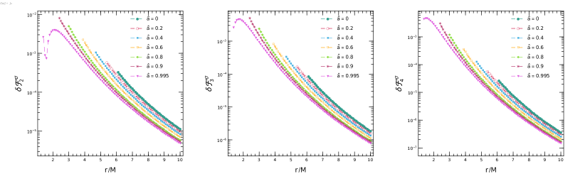
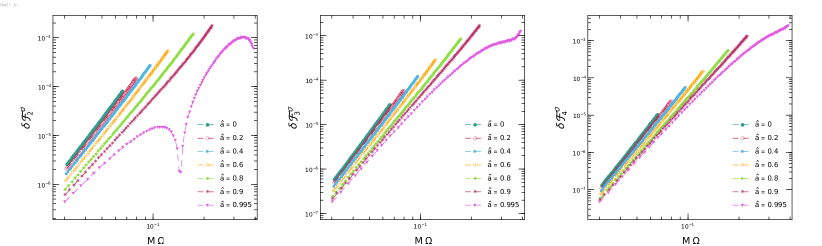
Figure 2: Top panels: The spin-correction coefficient $\delta{\cal F}^{\sigma}_{\ell}$ [see Eqs. (101) and  (102)] as a function of the orbital radius (up to the ISCO) for different values of the spin $\hat{a}$ of the primary and for $\ell=2,3,4$ (from left to right), summing up to all values of $m$ such that $|m|\leq\ell$. Bottom panel: the same but for the fluxes as a function of the orbital frequency. An analogous plot for the total spin-correction $\delta\mathcal{F}^{\sigma}=\sum_{\ell=2}^{20}\delta{\cal F}^{\sigma}_{\ell}$ is presented in a companion paper Piovano:2020ooe . Data for the fluxes are available online webpage and on the BH Perturbation Toolkit webpage BHPToolkit . Note that, for nearly-extremal primary ($\hat{a}\gtrsim 0.99$), $\delta{\cal F}^{\sigma}_{2}$ is nonmonotonic near the ISCO, although near extremality $\ell=2$ is not the dominant spin correction to the flux Gralla:2016qfw and the total correction $\delta{\cal F}^{\sigma}$ is monotonic Piovano:2020ooe .

Having computed the fluxes, we can now proceed to determine the adiabatic orbital evolution and the orbital phase by solving Eqs. (100). We consider an inspiral starting at $\hat{r}=\hat{r}_{\rm start}$. Ideally, one would like to evolve the inspiral up to the ISCO. However, since the latter depends on $\sigma$, so it does the duration of the inspiral, also for a fixed value of $\hat{a}$. It would therefore be complicated to compare the phase evolution for different spins of the secondary. Thus, we chose to evolve the inspiral up to a reference end time $t_{\text{ref}}=t_{\text{end}}-1/2\text{ day}$, where $t_{\text{end}}$ is the time to reach the ISCO for a nonspinning secondary for a given value of $\hat{a}$. The offset of $1/2\text{ day}$ is chosen so that the evolution stops before the ISCO for any value of $\hat{a}$ and $\chi$.

Throughout the inspiral, the phase $\Phi(t)$ can be written as

$$\Phi(t)=\Phi^{0}(t)+\frac{\sigma}{q}\delta\Phi^{\sigma}(t)+{\cal O}(\sigma^{2}/q)\,,$$ (105)

where $\Phi^{0}(t)$ is the phase for a nonspinning secondary and $\delta\Phi^{\sigma}(t)$ is the change due to the ${\cal O}(\sigma)$ contribution. Note that, since $\sigma=q\chi$, the linear spin correction is independent of $q$ to the leading order, and it is therefore suppressed by a factor $q$ relative to $\Phi^{0}(t)={\cal O}(1/q)$. The coefficients $\delta\Phi^{\sigma}(t)$ were obtained by interpolating $\Phi(t)-\Phi^{0}(t)$ with a cubic polynomial in $\chi$ as follows

$$\Phi(t)-\Phi^{0}(t)=a_{0}+\chi a_{1}+q\chi^{2}a_{2}+q^{2}\chi^{3}a_{3}\,,$$ (106)

where $a_{i}$ are the fit coefficients, with $a_{0}\approx 0$. The reported values of $a_{1}\equiv\delta\Phi^{\sigma}(t)$ are robust against the truncation order of the fit.

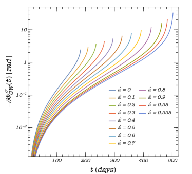
Figure 3: Time evolution of the linear spin corrections to the GW phase $\delta\Phi_{\text{GW}}^{\sigma}(t)$ for different values of $\hat{a}$.

The orbital phase $\Phi(t)$ is then related to the GW phase of the dominant mode by $\Phi_{\rm GW}(t)=2\Phi(t)$. The GW phase as a function of time is shown in Fig. 3 for various values of $\hat{a}$. Figure 4 also shows the phase difference $\Phi_{\text{GW}}(t_{\text{ref}})-\Phi^{0}_{\text{GW}}(t_{\text{ref}})$ computed at $t_{\text{ref}}$ as a function of the spin $\chi$, showing that it is linear to excellent accuracy. Although we only present the range $|\chi|\leq 2$, the phase difference is linear provided $|\sigma|\ll 1$, i.e. $|\chi|\ll 1/q$, as expected.

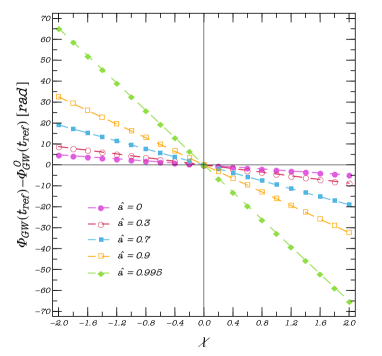
Figure 4: Phase difference $\Phi_{\text{GW}}(t_{\text{ref}})-\Phi_{\text{GW}}^{0}(t_{\text{ref}})$ between a spinning and nonspinning secondary as a function of $\chi$, calculated at $t_{\text{ref}}=t_{\text{end}}-1/2\text{ day}$, where $t_{\text{end}}$ is the time to reach the ISCO for a nonspinning secondary. Note that the curves are linear to an excellent accuracy, showing that $\Phi_{\text{GW}}(t_{\text{ref}})-\Phi_{\text{GW}}^{0}(t_{\text{ref}})\propto\chi$.

$\hat{a}$	$\delta\Phi^{\sigma}_{\rm GW}(t_{\text{ref}})[\text{rad}]$	$\Delta\chi$
0	-2.416	-0.414
0.1	-2.962	-0.338
0.2	-3.606	-0.277
0.3	-4.367	-0.229
0.4	-5.277	-0.189
0.5	-6.379	-0.157
0.6	-7.748	-0.129
0.7	-9.522	-0.105
0.8	-12.013	-0.0832
0.9	-16.215	-0.0617
0.95	-20.328	-0.0492
0.97	-23.271	-0.0430
0.990	-29.201	-0.0342
0.995	-32.570	-0.0307

Table 2: Spin corrections to the phase $\delta\Phi^{\sigma}_{\rm GW}(t_{\text{ref}})$ and its inverse (which gives the resolution on a measurement of $\chi$ according to criterion (109) with $\alpha=1$) for different values of $\hat{a}$.

The values of $\delta\Phi^{\sigma}_{\rm GW}(t_{\text{ref}})$ (i.e., the slope of the lines shown in Fig. 4) for different values of $\hat{a}$ are given in Table 2 and plotted in Ref. Piovano:2020ooe . We fitted these data with two different fits. The first one is

$$\delta\Phi^{\sigma}_{\rm GW}(t_{\rm ref})=\sum^{3}_{i=0}b_{i}(1-\hat{a}^{2})^{i/2}+b_{4}\hat{a}\ ,$$ (107)

where $b_{0}=38.44,b_{1}=-90.36,b_{2}=99.43,b_{3}=-44.95,b_{4}=1.91$. This fit is accurate within $5\%$ in the whole range $\hat{a}\in[0,0.995]$, with better accuracy at large $\hat{a}$. The second fit is

$$\delta\Phi^{\sigma}_{\rm GW}(t_{\rm ref})=\left\{\begin{array}[]{lll}\sum_{i=0}^{3}d_{i}\hat{a}^{i}&&\hat{a}\leq 0.7\\ \sum_{i=0}^{3}e_{i}(1-\hat{a}^{2})^{i/2}&&0.7\leq\hat{a}<0.995\end{array}\right.\ ,$$ (108)

where $d_{0}=-2.40$, $d_{1}=-5.70$, $d_{2}=0.13$, $d_{3}=-9.25$, and $e_{0}=-41.42$, $e_{1}/e_{0}=-2.49$, $e_{2}/e_{0}=3.30$, $e_{3}/e_{0}=-2.47$. This piecewise fit is accurate within $1\%$ in the whole range $\hat{a}\in[0,0.995]$.

Finally, we note that the order of magnitude of our dephasing is consistent with previous results that used approximated waveforms. In particular, our dephasing is compatible with the results of Refs. Barack:2006pq ; Huerta:2011kt that used “kludge” waveforms, and it agrees within a factor $\approx 2$, with the results of Ref. Yunes:2010zj , which used effective-one-body waveforms to model the EMRI signal.

VI.2 Minimum resolvable spin of the secondary

In a companion paper Piovano:2020ooe we briefly discussed how the above results can be used to place a constraint on the spin of the secondary in a model-independent fashion, i.e. without assuming any property of the secondary other than its mass and spin. Here we take the opportunity to extend that discussion.

Measuring the binary parameters from an EMRI signal is a challenging and open problem Huerta:2011kt ; Babak:2017tow ; Chua:2019wgs , which requires developing accurate waveform models, performing a statistical analysis that can account for correlations among the waveform parameters, and also taking into account that the EMRI events in LISA might overlap with several (possibly louder) simultaneous signals from supermassive BH coalescences and other sources Audley:2017drz ; Chua:2019wgs ; LISADataChallenge .

Postponing a data-analysis study for a follow-up work, here we estimate the minimum resolvable $\chi$ by computing the uncertainty on $\chi$ which would lead to a total GW dephasing $\approx 1\,{\rm rad}$. A larger dephasing would substantially impact a matched-filter search, leading to a significant loss of detected events and potentially to systematics in the parameter estimation Lindblom:2008cm .

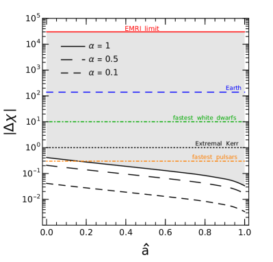
Figure 5: Resolution $|\Delta\chi|$ on a GW measurement of the spin of the EMRI secondary obtained saturating the criterion (109). A measured GW dephasing at the level of $\alpha\,{\rm rad}$ would probe the region above each curve. As a reference, we mark with horizontal lines some typical values of $\chi$ for astrophysical objects. Our analysis is valid for $\chi\ll 1/q\approx 3\times 10^{4}$ (continuous horizontal red line).

Let us then suppose that the EMRI masses, the spin of the primary BH $\hat{a}$, and the other waveform parameters except $\chi$ are known, i.e. we consider two waveforms which differ only by the value of the spin of the secondary, $\chi_{A}$ and $\chi_{B}$, respectively. The minimum difference $\Delta\chi=\chi_{B}-\chi_{A}$ which would lead to a difference in phase larger than $\alpha\,{\rm radiant}$ is Piovano:2020ooe

$$|\Delta\chi|>\frac{\alpha}{|\delta\Phi^{\sigma}_{\rm GW}|}\ .$$ (109)

The critical value is shown in the last column of Table 2 as a function of the primary spin $\hat{a}$ and assuming the $1$-radiant condition, i.e. $\alpha=1$. Based on previous analysis in a similar context Datta:2019epe , we expect that more stringent constraints would arise by computing the mismatch $\mathcal{M}$ between two waveforms and requiring $\mathcal{M}\gtrsim 1/(2\rho^{2})$ Flanagan:1997kp ; Lindblom:2008cm where $\rho$ is the signal-to-noise ratio of the EMRI signal. This would suggest using $\alpha<1$ for our estimates, although we shall adopt the more standard and conservative requirement and use $\alpha=1$.

Figure 5 shows the minimum resolution $|\Delta\chi|$ [obtained saturating Eq. (109)] as a function of the primary spin. For each chosen value of $\alpha$, the area above the corresponding curve identifies binary configurations producing a measurable dephasing according to our simplified analysis. In other words, the spin $\chi$ of a secondary can be measured with a relative error $\Delta\chi/\chi$.

It is interesting to compare such resolution with typical values of $\chi$ for known astrophysical objects. If the secondary is a Kerr BH, then $|\chi|\leq 1$. For the fastest millisecond pulsars, $\chi\approx 0.3$, although fast spinning pulsars are all in strongly-accreting binary systems, whereas isolated pulsars are expected to spin more slowly. However, $\chi$ can be much larger than unity for other objects. For example, a ball of radius $1\text{\,}\mathrm{cm}$ and mass $1\text{\,}\mathrm{kg}$ making one rotation per second has $\chi\approx 1\times 10^{17}$. Astrophysical objects do not reach such extreme values, but can have $\chi\gg 1$ Hartl:2002ig . For example, $\chi\approx 140$ for Earth, and $\chi\approx 10$ for the fastest white dwarfs in accreting binary systems. The above reference values are shown in Fig. 5 by horizontal lines.

Note that $|\Delta\chi|<1$ in all cases, and therefore our simplified analysis suggests that the spin of a rapidly spinning Kerr secondary could be measured with an accuracy greater than $100\%$.

VI.3 Model-independent constraints on “superspinars”

Compact dark objects which exceed the Kerr bound $|\chi|\leq 1$ (so-called “superspinars”) were suggested to arise generically in high-energy modifications to general relativity such as string theories Gimon:2007ur . Our results of Fig. 5 show that the typical resolution on $\chi$ achievable with an EMRI detection can be used to rule out (or detect) superspinars in a large region of the parameter space Piovano:2020ooe . For example, if $\chi\approx\hat{a}\approx(0.5-0.7)$, a measurement with absolute error $\Delta\chi$ would exclude $\chi>1$ at $3\sigma$ confidence level. This is particularly interesting in light of the fact that no theoretical upper bound is expected for superspinars, besides, possibly, those coming from the ergoregion instability Pani:2010jz ; Maggio:2017ivp ; Maggio:2018ivz ; Roy:2019uuy . A measurement of $\chi$ at the level reported above can thus potentially probe a vast region of the parameter space for superspinars Piovano:2020ooe .

In principle, a putative EMRI measurement of $|\chi|>1$ could still be degenerate with the secondary being a neutron star or a white dwarf. Given the theoretical upper bound on the maximum mass of such objects, an EMRI measurement of $\mu$ larger than $3M_{\odot}$ (resp. $\sim 1.4M_{\odot}$) would exclude a standard origin for the superspinar, as a neutron star (resp. a white dwarf). Similarly, no compact object spinning above the Kerr bound is know with $\mu\ll M_{\odot}$.

Moreover, even within the allowed, narrow, mass ranges, isolated compact stars feature spins smaller than the Kerr bound. Fast rotating neutron stars or white dwarfs are expected to evolve in accreting systems. For example, the fastest spinning white dwarf to date has $\chi\approx 10$, but it is strongly accreting from a binary companion 1997A&A…317..815B . Interestingly, all the observed fast rotating neutron stars rotate consistently below their theoretical maximum set by the mass shedding limit. While no solid explanation does exist to bridge this gap, EMRIs can provide a new window to discover neutron stars spinning close to the mass-shedding limit. Finally, less compact objects, such as brown dwarfs, might also have spin larger then the Kerr bound, but can be easily distinguishable from exotic superspinars, as they are tidally disrupted much before reaching the ISCO.

Finally, in the context of our study one could wonder whether it is theoretically consistent to study a secondary superspinar around a primary Kerr BH. This is indeed the case in two scenarios (see Ref. Cardoso:2019rvt for a review): a) if superspinars arise within general relativity in the presence of exotic matter fields, in such case both Kerr BHs and superspinars can co-exist in the spectrum of solutions of the theory; b) if superspinars arise in high-energy modified theories of gravity such as string theories, as originally proposed Gimon:2007ur . In the latter case it is natural to expect that high-energy corrections which are relevant for the secondary might be negligible for the primary. Indeed, in an effective-field-theory approach high-energy corrections to general relativity modify the Einstein-Hilbert action with the inclusion of higher-order curvature terms of the form Berti:2015itd ; Barack:2018yly

$$R+...+\beta(R_{abcd})^{n}+...\,,\quad n>1$$ (110)

where $R$ is the Ricci scalar, $R_{abcd}$ schematically denotes terms that depend on the Riemann tensor, and $\beta$ is a coupling constant with dimensions of a $(\text{length})^{2(n-1)}$. In these theories relative corrections to the metric of a compact object of size $\sim L$ are of the order of Barausse:2014tra

$$\frac{\beta}{L^{2(n-1)}}\,,$$ (111)

or some power thereof. Thus, the difference between the high-curvature corrections of the secondary relative to those of the primary scales as

$$\sim\frac{M^{2(n-1)}}{\mu^{2(n-1)}}=q^{2(1-n)}\gg 1\,.$$ (112)

This heuristically shows the obvious fact that in an EMRI the secondary is much more affected by the high-curvature corrections than the primary, especially for high-order terms (i.e., higher values of $n$).

In certain high-curvature corrections to general relativity, the secondary might also be charged under new fundamental fields, in which case there is also extra emission (in particular there could be dipolar, $\ell=1$, fluxes) Pani:2011xj ; Cardoso:2018zhm ; Maselli:2020zgv .

VII Conclusion and future work

We have studied the GW fluxes and the adiabatic evolution of a spinning point particle in circular, equatorial motion around the Kerr background and with spin (anti)aligned to that of the central BH. Our results for the fluxes agree with those previously appeared in the literature, whereas the computation of the GW phase in Kerr spacetime is novel .

Since the EMRI dynamics does not depend on the nature of the secondary but only on its multiple moments, the GW signal can be used to derive model-independent constraints on the secondary, for example to measure the spin of a Kerr secondary, or to distinguish whether the secondary is a fast spinning BH or a slowly-spinning neutron star, or also whether the secondary satisfies the Kerr bound or is a superspinar Piovano:2020ooe .

This work represents a first step in the analysis of the impact of the secondary spin on EMRI’s evolution, in parallel with recent work along related directions. Future work will include extensions to generic orbits (e.g., along the lines of Ref. Witzany:2019nml ), misaligned spins (which introduce precession Tanaka:1996ht ; Bini:2006pc ; Dolan:2013roa ; Ruangsri:2015cvg ), and the development of data analysis approaches Chua:2019wgs to assess the detectability of such effects. In particular, it is important to assess the role of parameter correlations in the measurement of small effects such as the spin of the secondary, as discussed in Ref. Huerta:2011kt . A complete account of dissipative effects in the case of a spinning secondary would also require to consider the spin evolution due to self-force effects, which is a more challenging problem, especially for generic orbits Akcay:2019bvk . Moreover, an important extension of this work is to include the contribution of the conservative first-order self-force on the equations of motion Burko:2003rv ; Burko:2015sqa ; Warburton:2017sxk and study how this affects the ${\cal O}(\sigma)$ in the GW signal.

Another interesting extension is to include the quadrupole moment of the secondary Hinderer:2013uwa ; Steinhoff:2012rw ; Bini:2014xyr . Compared to the spin, this effect is suppressed by a further power of the mass ratio and is probably negligible for EMRI detection with LISA, although a rigorous study is required to assess whether neglecting this term can affect parameter estimation for the loudest events. Furthermore, since the quadrupole moment of a Kerr BH is uniquely determined in terms of its mass a spin, measuring the quadrupole of the secondary would allow for model-independent tests of the BH no-hair theorem.

Finally, more theoretical related work includes nonintegrability and chaotic motion for generic values of the spin Zelenka:2019nyp ; Lukes-Gerakopoulos:2016udm ; Hartl:2002ig , although these effects might require extremely high values for the spin of the secondary and should not be directly relevant for the phenomenology of EMRI signals detectable with LISA.

Appendix A Sasaki-Nakamura equation

In this and in the following appendix we provide further technical details on the formalisms that we use in Secs. IV-V to compute the GW fluxes.

The homogeneous Teukolsky equation is an example of stiff differential problem, with the solutions (77)-(78) rapidly diverging at infinity due to the long-range character of the potential. High accuracy solutions require therefore time-consuming numerical integrations. A substantial improvement in this direction has been achieved by Sasaki and Nakamura, finding a suitable transformation which maps the homogeneous Teukolsky equation to an equivalent form with a short-range potential that is easier to solve numerically Sasaki:1981sx . The SN equation is given by (we remind that hatted quantities are dimensionless)

$$\bigg{[}f(\hat{r})^{2}\frac{\mathrm{d}^{2}}{\mathrm{d}\hat{r}^{2}}+f(\hat{r})\bigg{(}\frac{\mathrm{d}f(\hat{r})}{\mathrm{d}\hat{r}}-F(\hat{r})\bigg{)}\frac{\mathrm{d}}{\mathrm{d}\hat{r}}-U(\hat{r})\bigg{]}X_{\ell m\hat{\omega}}=0\ ,$$ (113)

with $f(\hat{r})=\frac{\mathrm{d}\hat{r}}{\mathrm{d}\hat{r}^{*}}=\frac{\Delta}{\hat{r}^{2}+\hat{a}^{2}}$. The coefficient $F(\hat{r})$ is defined as

$$F(\hat{r})=\frac{\eta(\hat{r})_{,\hat{r}}}{\eta(\hat{r})}\frac{\Delta}{\hat{r}^{2}+\hat{a}^{2}}\ ,$$ (114)

where ${}_{,\hat{r}}$ denotes the derivative with respect to $\hat{r}$ and

$$\eta(\hat{r})=c_{0}+\frac{c_{1}}{\hat{r}}+\frac{c_{2}}{\hat{r}^{2}}+\frac{c_{3}}{\hat{r}^{3}}+\frac{c_{4}}{\hat{r}^{4}}\ ,$$ (115)

with

$$c_{0} =-12i\hat{\omega}+\lambda_{\ell m\hat{\omega}}(\lambda_{\ell m\hat{\omega}}+2)-12\hat{a}\hat{\omega}(\hat{a}\hat{\omega}-m)\ ,$$ (116)

$$c_{1} =8i\hat{a}[3\hat{a}\hat{\omega}-\lambda_{\ell m\hat{\omega}}(\hat{a}\hat{\omega}-m)]\ ,$$ (117)

$$c_{2} =-24i\hat{a}(\hat{a}\hat{\omega}-m)+12\hat{a}^{2}[1-2(\hat{a}\hat{\omega}-m)^{2}]\ ,$$ (118)

$$c_{3} =24i\hat{a}^{3}(\hat{a}\hat{\omega}-m)-24\hat{a}^{2}\ ,$$ (119)

$$c_{4} =12\hat{a}^{4}\ .$$ (120)

The function $U(\hat{r})$ in Eq. (113) reads

$$U(\hat{r})=\frac{\Delta U_{1}(\hat{r})}{(\hat{r}^{2}+\hat{a}^{2})^{2}}+G(\hat{r})^{2}+\frac{\Delta G(\hat{r})_{,\hat{r}}}{\hat{r}^{2}+\hat{a}^{2}}-F(\hat{r})G(\hat{r})\ ,$$ (121)

where

$$G(\hat{r}) =-\frac{2(\hat{r}-1)}{\hat{r}^{2}+\hat{a}^{2}}+\frac{\hat{r}\Delta}{(\hat{r}^{2}+\hat{a}^{2})^{2}}\ ,$$ (122)

$$U_{1}(\hat{r}) =V(\hat{r})+\frac{\Delta^{2}}{\beta}\Big{[}\Big{(}2\alpha+\frac{\beta_{,\hat{r}}}{\Delta}\Big{)}_{\!\!,\hat{r}}-\frac{\eta(\hat{r})_{,\hat{r}}}{\eta(\hat{r})}\Big{(}\alpha+\frac{\beta_{,\hat{r}}}{\Delta}\Big{)}\Big{]}\ ,$$ (123)

$$\alpha =-iK(\hat{r})\frac{\beta}{\Delta^{2}}+3iK(\hat{r})_{,\hat{r}}+\lambda_{\ell m\hat{\omega}}+\frac{6\Delta}{\hat{r}^{2}}\ ,$$ (124)

$$\beta =2\Delta\Big{[}-iK(\hat{r})+\hat{r}-1-\frac{2\Delta}{\hat{r}}\Big{]}\ .$$ (125)

The two functions $K(\hat{r})$ and $V(\hat{r})$ are the same introduced for the Teukolsky radial equation (74).

The SN equation admits two linearly independent solutions, $X^{\textup{in}}_{\ell m\hat{\omega}}$ and $X^{\textup{up}}_{\ell m\hat{\omega}}$, which behave asymptotically as

$$X^{\textup{in}}_{\ell m\hat{\omega}}\sim\begin{cases}e^{-i\hat{\kappa}\hat{r}^{\ast}}\quad&\hat{r}\to\hat{r}_{+}\\ A^{\textup{out}}_{\ell m\hat{\omega}}e^{i\hat{\omega}\hat{r}^{\ast}}+A^{\textup{in}}_{\ell m\hat{\omega}}e^{-i\hat{\omega}\hat{r}^{\ast}}\quad&\hat{r}\to\infty\end{cases}\,,$$ (126)

$$X^{\textup{up}}_{\ell m\hat{\omega}}\sim\begin{cases}C^{\textup{out}}_{\ell m\hat{\omega}}e^{i\hat{\kappa}\hat{r}^{\ast}}+C^{\textup{in}}_{\ell m\hat{\omega}}e^{-i\hat{\kappa}\hat{r}^{\ast}}\quad\,&r\to r_{+}\\ e^{i\hat{\omega}\hat{r}^{\ast}}\,\quad&\hat{r}\to\infty\end{cases}\,.$$ (127)

The solutions of the Teukolsky and SN equations are related by:

$$R^{\textup{in},\textup{up}}_{\ell m\hat{\omega}}(\hat{r}) =\frac{1}{\eta}\bigg{[}\bigg{(}\alpha+\frac{\beta_{,\hat{r}}}{\Delta}\bigg{)}Y^{\textup{in},\textup{up}}_{\ell m\hat{\omega}}-\frac{\beta}{\Delta}{Y^{\textup{in},\textup{up}}_{\ell m\hat{\omega}}}_{\!\!,\hat{r}}\bigg{]}\ ,$$ (128)

$$Y^{\textup{in},\textup{up}}_{\ell m\hat{\omega}} =\frac{\Delta}{\sqrt{\hat{r}^{2}+\hat{a}^{2}}}X^{\textup{in},\textup{up}}_{\ell m\hat{\omega}}\ .$$ (129)

With the above normalization of the solutions $X^{\textup{in}}_{\ell m\hat{\omega}}$ $X^{\textup{up}}_{\ell m\hat{\omega}}$, these transformations allow to fix the arbitrary constants $D^{\textup{tran}}_{\ell m\hat{\omega}}$ and $B^{\textup{tran}}_{\ell m\omega}$ [cf. Eq. (86)] as Mino:1997bx :

$$D^{\textup{tran}}_{\ell m\hat{\omega}}=-\frac{4\hat{\omega}^{2}}{c_{0}}\ ,\qquad\quad B^{\textup{tran}}_{\ell m\hat{\omega}}=\frac{1}{d_{\ell m\hat{\omega}}}\ ,$$ (130)

where

$$d_{\ell m\hat{\omega}}=4\sqrt{2\hat{r}_{+}}[(2-6i\hat{\omega}-4\hat{\omega}^{2})\hat{r}_{+}^{2}+(3i\hat{a}m-4$$

$$+4\hat{a}\hat{\omega}m+6i\hat{\omega})\hat{r}_{+}-\hat{a}^{2}m^{2}-3iam+2]\ ,$$ (131)

and the coefficient $c_{0}$ is given in Eq. (116).

The numerical values of $X^{\textup{in}}_{\ell m\hat{\omega}}$ (resp. $X^{\textup{up}}_{\ell m\hat{\omega}}$) are obtained by integrating Eq. (113) from $\hat{r}_{+}$ (resp. infinity) up to infinity (resp. $\hat{r}_{+}$) using the boundary conditions (126) (resp. (127)). In this work we have derived the boundary conditions for the homogeneous SN equation in terms of explicit recursion relations which can be truncated at arbitrary order (see Sec. A.1). We finally transform back $X^{\textup{in}}_{\ell m\hat{\omega}},X^{\textup{up}}_{\ell m\hat{\omega}}$ to the Teukolsky solutions using Eq. (128). The amplitude $B^{\textup{in}}_{\ell m\hat{\omega}}$ can be obtained from the Wronskian $W_{\hat{r}}$ at a given orbital separation.

A.1 Boundary conditions for the SN equation in terms of recursion relations

We have derived accurate boundary conditions by looking for series expansions of the master equation at the outer horizon $\hat{r}_{+}$ and at infinity. To this aim we have studied the singularities on the real axis of Eq. (113), which can be recast in the form

$$\Delta^{2}\frac{d^{2}X_{\ell m\hat{\omega}}}{d\hat{r}^{2}}+\Delta\overline{F}(\hat{r})\frac{dX_{\ell m\hat{\omega}}}{d\hat{r}}+\overline{U}(\hat{r})X_{\ell m\hat{\omega}}=0\ ,$$ (132)

where

$$\overline{F}(\hat{r}) =(\hat{r}^{2}+\hat{a}^{2})\bigg{(}\frac{\mathrm{d}f(\hat{r})}{\mathrm{d}\hat{r}}-F(\hat{r})\bigg{)}\ ,$$ (133)

$$\overline{U}(\hat{r}) =-(\hat{r}^{2}+\hat{a}^{2})^{2}U(\hat{r})\ .$$ (134)

Moreover

$$F(\hat{r}_{\pm}) =0\ , \quad F(\hat{r}) \xrightarrow[\hat{r}\to\infty]{}0\ ,$$ (135)

$$U(\hat{r}_{+}) =-\hat{\kappa}^{2}\ , \quad U(\hat{r}) \xrightarrow[\hat{r}\to\infty]{}-\hat{\omega}^{2}\ .$$ (136)

Since the functions $\overline{F}(\hat{r})$ and $\overline{U}(\hat{r})$ are analytic on the positive real axis, it turns out that the Eq. (113) has three singularities: two at the horizons $\hat{r}=\hat{r}_{-}$ and $\hat{r}=\hat{r}_{+}$, both of which are regular singularities, and one at $\hat{r}=\infty$ which is an irregular singularity of rank $1$. By Fuchs theorem, the solutions of the SN equation around $\hat{r}_{+}$ can be written as Frobenius series, with radius of convergence

$$\hat{r}_{+}-\hat{r}_{-}=2\sqrt{1-\hat{a}^{2}}\ .$$ (137)

For $\hat{r}=\infty$ or $\hat{a}=1$ (for which $\hat{r}_{+}=\hat{r}_{-}$) the boundary conditions can be written in terms of asymptotic expansions.

A.1.1 Boundary condition at the horizon

To compute the boundary conditions at the outer horizon $\hat{r}_{+}$, it is convenient to recast the SN equation as

$$(\hat{r}-\hat{r}_{+})^{2}\frac{d^{2}X_{\ell m\hat{\omega}}}{d\hat{r}^{2}}+(\hat{r}-\hat{r}_{+})p_{H}(\hat{r})\frac{dX_{\ell m\omega}}{d\hat{r}}+q_{H}(\hat{r})X_{\ell m\hat{\omega}}=0$$ (138)

where

$$p_{H}(\hat{r}) =\bigg{(}\frac{\hat{r}^{2}+\hat{a}^{2}}{\hat{r}-\hat{r}_{-}}\bigg{)}\bigg{[}\frac{\mathrm{d}f(\hat{r})}{\mathrm{d}\hat{r}}-F(\hat{r})\bigg{]}\ ,$$ (139)

$$q_{H}(\hat{r}) =-\bigg{(}\frac{\hat{r}^{2}+\hat{a}^{2}}{\hat{r}-\hat{r}_{-}}\bigg{)}^{\!2}U(\hat{r})\ .$$ (140)

Following the Frobenius method we look for a power series solution of the form

$$X_{\ell m\hat{\omega}}=(\hat{r}-\hat{r}_{+})^{d}\displaystyle\sum_{n=0}^{\infty}a_{n}(\hat{r}-\hat{r}_{+})^{n}\ ,$$ (141)

where $d$ is one of the solutions of the indicial equation

$$I(d)=d(d-1)+p_{H}(\hat{r}_{+})d+q_{H}(\hat{r}_{+})=0\ .$$ (142)

For Eq. (113), the latter corresponds to

$$I(d)=d^{2}+\kappa^{2}\left(\frac{2\hat{r}_{+}}{\hat{r}_{+}-\hat{r}_{-}}\right)^{\!\!2}=0\ ,\quad\ \hat{\kappa}=\hat{\omega}-\frac{m\hat{a}}{2\hat{r}_{+}}\ .$$ (143)

Given $(d_{1},d_{2})$ two solutions of the above equation, their difference $d_{1}-d_{2}$ is neither zero nor an integer. We have therefore two linearly independent solutions such that

$$X_{\ell m\hat{\omega}}=\exp\bigg{\{}\pm i\hat{\kappa}\frac{2\hat{r}_{+}}{\hat{r}_{+}-\hat{r}_{-}}\log(\hat{r}-\hat{r}_{+})\bigg{\}}\displaystyle\sum_{n=0}^{\infty}a_{n}(r-r_{+})^{n}\ .$$ (144)

The recursion relation for the coefficients $a_{n}$ is (setting $a_{0}=1$)

$$a_{n}=-\frac{1}{I(d+n)}\displaystyle\sum_{k=0}^{n-1}\frac{(k+d)p_{H}^{(n-k)}(\hat{r}_{+})+q_{H}^{(n-k)}(r_{+})}{(n-k)!}a_{k}\ ,$$ (145)

where $p_{H}^{(k)}(\hat{r}_{+})$ and $q_{H}^{(k)}(\hat{r}_{+})$ are the $k$-th derivatives of the coefficients $p_{H}(\hat{r})$ and $q_{H}(\hat{r})$ with respect to $\hat{r}$, and calculated at $\hat{r}_{+}$. For $\hat{a}\leq 0.9$, the boundary conditions at the horizon have been calculated at $\hat{r}_{\text{in}}=\hat{r}_{+}+\epsilon$ with $\epsilon=10^{-3}$, while for higher spins we have fixed $\epsilon=10^{-5}$. To increase precision, we truncate compute the series coefficients up to $n=10$.

A.1.2 Boundary condition at infinity

Ordinary differential equations with irregular singularities of rank $1$, like the SN equation, admit general expressions for asymptotic expansions around such singularities (see Refs. Olver:1994:AEC ; Olver:1997:ASL and especially Ref. Olver:1974asymptotics for more details). To calculate the boundary conditions at infinity we rewrite the SN equation as

$$\frac{d^{2}X_{\ell m\hat{\omega}}}{d\hat{r}^{2}}+p_{\infty}(\hat{r})\frac{dX_{\ell m\hat{\omega}}}{d\hat{r}}+q_{\infty}(\hat{r})X_{\ell m\hat{\omega}}=0\ ,$$ (146)

where

$$p_{\infty}(\hat{r}) =\frac{(\hat{r}^{2}+\hat{a}^{2})}{\Delta}\bigg{[}\frac{\mathrm{d}f(\hat{r})}{\mathrm{d}\hat{r}}-F(\hat{r})\bigg{]}\ ,$$ (147)

$$q_{\infty}(\hat{r}) =-\bigg{(}\frac{\hat{r}^{2}+\hat{a}^{2}}{\Delta}\bigg{)}^{\!2}U(\hat{r})\ .$$ (148)

The functions $p_{\infty}(\hat{r})$ and $q_{\infty}(\hat{r})$ are analytic on the positive real axis, so the series

$$p_{\infty}(\hat{r}) =\displaystyle\sum_{n=0}^{\infty}\frac{1}{n!}\frac{p_{\infty}^{(n)}}{\hat{r}^{n}}\ ,\qquad q_{\infty}(\hat{r}) =\displaystyle\sum_{n=0}^{\infty}\frac{1}{n!}\frac{q_{\infty}^{(n)}}{\hat{r}^{n}}\ ,$$

converge, with $p_{\infty}^{(n)}$ and $q_{\infty}^{(n)}$ being the $n$-th derivatives of the coefficients $p_{\infty}$ and $q_{\infty}$ with respect to $\hat{r}$. If at least one of $p_{\infty}^{(0)}$, $q_{\infty}^{(0)}$ or $q_{\infty}^{(1)}$ is nonzero, the formal solution is given by

$$X_{\ell m\hat{\omega}}=e^{\gamma\hat{r}}\hat{r}^{\xi}\displaystyle\sum_{n=0}^{\infty}\frac{b_{n}}{\hat{r}^{n}}\ ,$$ (149)

where $\gamma$ is one of the solutions of the characteristic equation

$$\gamma^{2}+p^{(0)}_{\infty}\gamma+q^{(0)}_{\infty}=0\ ,$$ (150)

while

$$\xi=-\frac{p_{\infty}^{(1)}\gamma+q_{\infty}^{(1)}}{p_{\infty}^{(0)}+2\gamma}\ .$$ (151)

For the SN equation

$$p_{\infty}^{(0)} =0=p_{\infty}^{(1)}\ ,\qquad q_{\infty}^{(0)}=\omega^{2}\ ,\qquad q_{\infty}^{(1)}=4\hat{\omega}^{2}\ ,$$ (152)

$$\gamma^{2} +\hat{\omega}^{2}=0\ ,\qquad\xi=-\frac{q_{\infty}^{(1)}}{2\gamma}=\pm 2i\hat{\omega}\ .$$ (153)

Therefore, we have two series solutions

$$X_{\ell m\hat{\omega}}=\exp\{\pm i\hat{\omega}[\hat{r}+2\log(\hat{r})]\}\displaystyle\sum_{n=0}^{\infty}\frac{b_{n}}{\hat{r}^{n}}\,.$$ (154)

The general recursion relation for the coefficients $b_{n}$ is (we set again $b_{0}=1$)

$$(p_{\infty}^{(0)}+2\gamma)nb_{n}=(n-\xi)(n-1-\xi)b_{n-1}+$$

$$+\displaystyle\sum_{k=1}^{n}\Big{[}\gamma p_{\infty}^{(k+1)}+q_{\infty}^{(k+1)}-(n-k-\xi)p_{\infty}^{(k)}\Big{]}b_{n-k}\ .$$ (155)

It can be proved that the series solutions constructed in this way diverge, and they have to be considered as asymptotic expansions. However, these solutions are unique and linearly independent. We computed the series coefficients up to $n=13$.

A.1.3 Cross check of the boundary conditions with Ref. Gralla:2015rpa

We compared our boundary conditions with the ones used in Ref. Gralla:2015rpa , which are in form

$$e^{\pm i\hat{\kappa}\hat{r}^{\ast}}\displaystyle\sum_{n=0}^{\infty}a^{\text{H}}_{n}(\hat{r}-\hat{r}_{+})^{n}\,,$$ (156)

$$e^{\pm i\hat{\omega}\hat{r}^{\ast}}\displaystyle\sum_{n=0}^{\infty}a^{\infty}_{n}\frac{1}{(\hat{\omega}\hat{r})^{n}}\,.$$ (157)

First, we notice that the tortoise coordinate $\hat{r}^{\ast}(\hat{r})$ at the boundaries can be written as

$$\hat{r}^{\ast}(\hat{r}) \sim\hat{r}+2\ln(\hat{r})-2\ln(2)\,,$$ (158)

$$\hat{r}^{\ast}(\hat{r}) \sim\frac{2\hat{r}_{+}}{\hat{r}_{+}-\hat{r}_{-}}\ln(\hat{r}-\hat{r}_{+})+\delta r^{*}(r_{+})\,,$$ (159)

at $\hat{r}\to\infty$ and $\hat{r}\to\hat{r}_{+}$, respectively, and where we defined

$$\delta\hat{r}^{*}(\hat{r}_{+}) \equiv-2\ln(2)-\frac{2\hat{r}_{-}}{\hat{r}_{+}-\hat{r}_{-}}\ln(\hat{r}_{+}-\hat{r}_{-})+\hat{r}_{+}\,.$$ (160)

If we multiply Eq. (144) by the phase factor $\exp\{\pm i\hat{\kappa}\delta\hat{r}^{*}(\hat{r}_{+})\}$ and Eq. (154) by $\exp\{\pm i\hat{\omega}[-2\ln(2)]\}$, our boundary conditions have the same modulus and phase as those in Ref. Gralla:2015rpa for all the values of the parameters space we have considered, up to numerical error. In the worst case, for $\hat{a}=0.995$ and $\ell=20$ at the ISCO, the fractional difference in both modulus and phase is at most of one part in $10^{10}$, and typically much smaller.

Since the solutions by means of series expansion of an ordinary differential equation are uniquely determined a part for a constant complex factor, the boundary conditions (144) and (154) are consistent with the ones of Ref. Gralla:2015rpa .

Appendix B Teukolsky source term

B.1 Spinning particle on a general bound orbit

The source term of the Teukolsky equation reads

$$\mathcal{T}_{\ell m\hat{\omega}}=4\!\int\!\!\mathrm{d}\hat{t}\mathrm{d}\theta\sin\theta\mathrm{d}\phi\frac{\left(B^{\prime}_{2}+{B^{\prime}_{2}}^{*}\right)}{\bar{\rho}\rho^{5}}\!\!\prescript{}{-2}{S^{\hat{a}\hat{\omega}}_{\ell m}}e^{-i(m\phi+\hat{\omega}\hat{t})}\ ,$$ (161)

where the functions $B^{\prime}_{2}$ and ${B^{\prime}_{2}}^{*}$ are defined as

$$B^{\prime}_{2} =-\frac{1}{2}\rho^{8}\bar{\rho}\mathcal{L}_{-1}\bigg{[}\frac{1}{\rho^{4}}\mathcal{L}_{0}\bigg{[}\frac{T_{nn}}{\rho^{2}\bar{\rho}}\bigg{]}\bigg{]}+$$

$$-\frac{1}{2\sqrt{2}}\Delta^{2}\rho^{8}\bar{\rho}\mathcal{L}_{-1}\bigg{[}\frac{\bar{\rho}^{2}}{\rho^{4}}J_{+}\bigg{[}\frac{T_{\overline{m}n}}{\Delta\rho^{2}\bar{\rho}^{2}}\bigg{]}\bigg{]}\ ,$$ (162)

$${B^{\prime}_{2}}^{*} =-\frac{1}{4}\Delta^{2}\rho^{8}\bar{\rho}J_{+}\bigg{[}\frac{1}{\rho^{4}}J_{+}\bigg{[}\frac{\bar{\rho}}{\rho^{2}}T_{\overline{m}\overline{m}}\bigg{]}\bigg{]}+$$

$$-\frac{1}{2\sqrt{2}}\Delta^{2}\rho^{8}\bar{\rho}J_{+}\bigg{[}\frac{\bar{\rho}^{2}}{\Delta\rho^{4}}\mathcal{L}_{-1}\bigg{[}\frac{T_{\overline{m}n}}{\rho^{2}\bar{\rho}^{2}}\bigg{]}\bigg{]}\ ,$$ (163)

with $J_{+}=\frac{\partial}{\partial\hat{r}}+\frac{iK}{\Delta}$ and

$$\rho =\frac{1}{\hat{r}-i\hat{a}\cos(\theta)}\ ,\qquad\quad\bar{\rho}=\frac{1}{\hat{r}+i\hat{a}\cos(\theta)} \ ,$$ (164)

$$\mathcal{L}_{s} =\frac{\partial}{\partial\theta}+\frac{m}{\sin(\theta)}-\hat{a}\hat{\omega}\sin(\theta)+s\cot(\theta) \ ,$$ (165)

$$\mathcal{L}_{s}^{\dagger} =\frac{\partial}{\partial\theta}-\frac{m}{\sin(\theta)}+\hat{a}\hat{\omega}\sin\theta+s\cot(\theta) \ .$$ (166)

The components $T_{nn},T_{\overline{m}n}$, and $T_{\overline{m}\overline{m}}$ are the projections of the stress-energy tensor with respect to the Newman-Penrose (NP) tetrad:

$$l^{\mu} =\sqrt{\frac{\Sigma}{\Delta}}\left(e^{\mu}_{(0)}+e^{\mu}_{(1)}\right)\ ,\quad n^{\mu}=\frac{1}{2}\sqrt{\frac{\Delta}{\Sigma}}\left(e^{\mu}_{(0)}-e^{\mu}_{(1)}\right)\ ,$$ (167)

$$m^{\mu} =\bar{\rho}\sqrt{\frac{\Sigma}{2}}\left(e^{\mu}_{(2)}+ie^{\mu}_{(3)}\right),\; \overline{m}^{\mu}=\rho\sqrt{\frac{\Sigma}{2}}\left(e^{\mu}_{(2)}-ie^{\mu}_{(3)}\right)\ ,$$ (168)

where, for example, $T_{nn}=n^{\mu}n^{\nu}T_{\mu\nu}$ Mino:1995fm . Henceforth we use the notation $S^{\hat{a}\hat{\omega}}_{\ell m}$ instead of $\!\prescript{}{-2}{S^{\hat{a}\hat{\omega}}_{\ell m}}$ for the spin-weighted spheroidal harmonics to reduce clutter in the notation.

All $\theta$-derivatives in $T_{nn},T_{\overline{m}n}$ and $T_{\overline{m}\overline{m}}$ can be removed by repeated integrations by parts and by making use of the following identity

$$\int_{0}^{\pi}\!h(\theta)\mathcal{L}_{s}[g(\theta)]\sin(\theta)\mathrm{d}\theta=-\int_{0}^{\pi}\!g(\theta)\mathcal{L}^{\dagger}_{s}[h(\theta)]\sin(\theta)\mathrm{d}\theta\ ,$$ (169)

with $h(\theta)$ and $g(\theta)$ regular functions. It is thus possible to write

$$\mathcal{T}_{\ell m\hat{\omega}}=\int\!\!\mathrm{d}t\mathrm{d}\theta\mathrm{d}\phi\Delta^{2}e^{i(\hat{\omega}\hat{t}-m\phi)}\big{(}\mathcal{T}_{nn}+\mathcal{T}_{\overline{m}n}+\mathcal{T}_{\overline{m}\overline{m}}\big{)}\ ,$$ (170)

with

$$\mathcal{T}_{nn}=-\frac{2}{\Delta^{2}\rho^{2}\bar{\rho}}\mathcal{L}^{\dagger}_{1}\bigg{[}\frac{1}{\rho^{4}}\mathcal{L}^{\dagger}_{2}\big{[}\rho^{3}S^{\hat{a}\hat{\omega}}_{\ell m}\big{]}\bigg{]}\!\sin(\theta)T_{nn}\ ,$$ (171)

$$\mathcal{T}_{\overline{m}n} =\frac{4}{\sqrt{2}}\frac{\overline{\rho}}{\rho^{2}}\mathcal{L}^{\dagger}_{2}\big{[}S^{\hat{a}\hat{\omega}}_{\ell m}\rho\overline{\rho}\big{]}J_{+}\bigg{[}\frac{T_{\overline{m}n}}{\Delta\rho^{2}\overline{\rho}^{2}}\bigg{]}\!\sin(\theta)+$$

$$+\frac{2}{\sqrt{2}}\frac{1}{\rho^{2}\bar{\rho}^{2}\Delta}\mathcal{L}^{\dagger}_{2}\bigg{[}\rho^{3}S^{\hat{a}\hat{\omega}}_{\ell m}\frac{\mathrm{d}}{\mathrm{d}\hat{r}}\bigg{(}\frac{\bar{\rho}^{2}}{\rho^{4}}\bigg{)}\bigg{]}\!\sin(\theta)T_{\overline{m}n}\ ,$$ (172)

$$\mathcal{T}_{\overline{m}\overline{m}}=-\rho^{3}S^{\hat{a}\hat{\omega}}_{\ell m}J_{+}\bigg{[}\frac{1}{\rho^{4}}J_{+}\bigg{[}\frac{\bar{\rho}}{\rho^{2}}T_{\overline{m}\overline{m}}\bigg{]}\bigg{]}\!\sin(\theta)\ .$$ (173)

It is convenient to expand the previous terms in order to isolate the derivatives of the projected stress-energy tensor with respect to $\hat{r}$ and the derivative of $S^{\hat{a}\hat{\omega}}_{\ell m}$ with respect to $\theta$. After some algebra, we get

$$\mathcal{T}_{nn}=-\frac{2\sin(\theta)}{\Delta^{2}\rho^{3}\bar{\rho}}\Big{[}\Big{(}\mathcal{L}^{\dagger}_{1}-2i\hat{a}\rho\sin(\theta)\Big{)}\mathcal{L}^{\dagger}_{2}S^{\hat{a}\hat{\omega}}_{\ell m}\Big{]}T_{nn}\ ,$$ (174)

$$\mathcal{T}_{\overline{m}n} =\frac{4\sin(\theta)}{\sqrt{2}}\bigg{\{}\partial_{\hat{r}}\bigg{[}\Big{(}\mathcal{L}^{\dagger}_{2}S^{\hat{a}\hat{\omega}}_{\ell m}+i\hat{a}\sin\theta(\bar{\rho}-\rho)S^{\hat{a}\hat{\omega}}_{\ell m}\Big{)}\frac{T_{\overline{m}n}}{\rho^{3}\Delta}\bigg{]}$$

$$+\bigg{[}\bigg{(}\frac{iK}{\Delta}+\rho+\bar{\rho}\bigg{)}\mathcal{L}^{\dagger}_{2}S^{\hat{a}\hat{\omega}}_{\ell m}$$

$$-\hat{a}\sin(\theta)\frac{K}{\Delta}(\bar{\rho}-\rho)S^{\hat{a}\hat{\omega}}_{\ell m}\bigg{]}\frac{T_{\overline{m}n}}{\rho^{3}\Delta}\bigg{\}}\ ,$$ (175)

$$\mathcal{T}_{\overline{m}\overline{m}} =\left\{-\partial^{2}_{\hat{r}}\!\left(\frac{\bar{\rho}}{\rho^{3}}T_{\overline{m}\overline{m}}\right)\!-2\partial_{\hat{r}}\!\left(\left(\frac{\bar{\rho}}{\rho^{2}}+\frac{\bar{\rho}}{\rho^{3}}\frac{iK}{\Delta}\right)T_{\overline{m}\overline{m}}\right)\right.$$

$$\left.+\frac{\bar{\rho}}{\rho^{3}}\!\left(\frac{\mathrm{d}}{\mathrm{d}\hat{r}}\!\left(\frac{iK}{\Delta}\right)\ -2\rho\frac{iK}{\Delta}+\frac{K^{2}}{\Delta^{2}}\right)\!T_{\overline{m}\overline{m}}\right\}\!\sin(\theta)S^{\hat{a}\hat{\omega}}_{\ell m}\ .$$ (176)

The stress-energy tensor for a spinning object is given by Tanaka:1996ht

$$T^{\mu\nu} =q\!\displaystyle\int\!\mathrm{d}\hat{\lambda}\Bigg{[}\frac{\delta^{(4)}_{x,z(\lambda)}}{\sqrt{-g}}u^{(\mu}v^{\nu)}-\nabla_{\sigma}\Bigg{(}S^{\sigma(\mu}v^{\nu)}\frac{\delta^{(4)}_{x,z(\lambda)}}{\sqrt{-g}}\Bigg{)}\Bigg{]}\ ,$$ (177)

where $\delta^{(4)}_{x,z(\lambda)}\equiv\prod_{\nu=0}^{4}\delta\big{(}x^{\nu}-z^{\nu}(\hat{\lambda})\big{)}$ and indices within parenthesis denote symmetrization. The tetrad components are Tanaka:1996ht

$$T^{(a)(b)}=q\!\int\!\!\frac{\mathrm{d}\hat{\lambda}}{\sqrt{-g}} \Big{[}u^{((a)}v^{(b))}\delta^{(4)}_{x,z(\lambda)}$$

$$-{e^{{(}(a)}}_{\nu}\,{e^{(b){)}}}_{\rho}\nabla_{\sigma}\!\left(S^{\sigma\nu}v^{\rho}\delta^{(4)}_{x,z(\lambda)}\right)\!\Big{]}\,.$$ (178)

The above equation can be written as

$$T^{(a)(b)} =q\!\int\!\frac{\mathrm{d}\hat{\lambda}}{\sqrt{-g}}\Big{[}\delta^{(4)}_{x,z(\lambda)}\!\left(u^{{(}(a)}v^{(b){)}}+\right.$$

$$\left.+{\omega_{(d)(c)}}^{{(}(a)}v^{(b){)}}S^{(d)(c)}-{\omega_{(d)(c)}}^{{(}(a)}S^{(b){)}(d)}v^{(c)}\right)+$$

$$-\partial_{\sigma}\!\left(S^{{(}(a)}v^{(b){)}}\delta^{(4)}_{x,z(\lambda)}\right)\!\Big{]}\ .$$ (179)

For bound orbits, it is useful to rewrite the energy-momentum tensor as

$$T^{(a)(b)} =\frac{1}{\sqrt{-g}}\delta^{(3)}_{\underline{x},\underline{x}(\hat{t})}\Big{(}\mathcal{P}^{(a)(b)}-\mathcal{S}^{t(a)(b)}\partial_{\hat{t}}\Big{)}+$$

$$+\frac{1}{\sqrt{-g}}\partial_{i}\Big{(}\mathcal{S}^{i(a)(b)}\delta^{(3)}_{\underline{x},\underline{x}(t)}\Big{)}\ ,$$ (180)

where $i=\{r,\theta,\phi\}$, $\delta^{(3)}_{\underline{x},\underline{x}(t)}=\delta\big{(}\hat{r}-\hat{r}(\hat{t})\big{)}\delta\big{(}\theta-\theta(t)\big{)}\delta\big{(}\phi-\phi(\hat{t})\big{)}$, and we defined

$$\mathcal{P}^{(a)(b)} \coloneqq q\left|\frac{\mathrm{d}\hat{t}}{\mathrm{d}\hat{\lambda}}\right|^{-1}\!\Big{(}u^{{(}(a)}v^{(b){)}}+{\omega_{(d)(c)}}^{{(}(a)}v^{(b){)}}S^{(d)(c)}$$

$$-\omega_{(d)(c)}{}^{{(}(a)}S^{(b){)}(d)}v^{(c)}\Big{)}\ ,$$ (181)

$$\mathcal{S}^{\sigma(a)(b)} \coloneqq-q\left|\frac{\mathrm{d}\hat{t}}{\mathrm{d}\hat{\lambda}}\right|^{-1}S^{\sigma{(}(a)}v^{(b){)}}\ .$$ (182)

To rewrite the stress-energy tensor we used the well-known property of the derivative of a Dirac delta:

$$\int_{-\infty}^{\infty}\!\mathrm{d}xh(x)\frac{\mathrm{d}}{\mathrm{d}x}\delta(x-x_{0})=-\left.\frac{\mathrm{d}h}{\mathrm{d}x}\right\rvert_{x=x_{0}}\,.$$ (183)

In this way, the stress-energy tensor can be interpreted as a linear differential operator that acts on the smooth functions inside of the Teukolsky source term.

We now need to project $T^{ab}$ with respect to the NP null tetrad. In the following, we will employ a reduced version of the NP tetrad:

$$\tilde{l}^{\mu} =\left(e^{\mu}_{(0)}+e^{\mu}_{(1)}\right)\,,\quad \tilde{n}^{\mu} =\frac{1}{2}\left(e^{\mu}_{(0)}-e^{\mu}_{(1)}\right)\,,$$ (184)

$$\tilde{m}^{\mu} =\frac{1}{\sqrt{2}}\left(e^{\mu}_{(2)}+ie^{\mu}_{(3)}\right)\,,\quad \tilde{k}^{\mu} =\frac{1}{\sqrt{2}}\left(e^{\mu}_{(2)}-ie^{\mu}_{(3)}\right)\,,$$ (185)

where $\tilde{k}^{\mu}$ is the complex conjugate of $\tilde{m}^{\mu}$. Taking into account that the $\hat{t}$ and $\phi$ coordinates in the Teukolsky source term are only present in the exponential, and using the definitions $T_{nn}=n^{\mu}n^{\nu}e_{\mu(a)}e_{\nu(b)}T^{(a)(b)}$ and so on, the projected components read

$$T_{nn} =\delta^{(3)}_{\underline{x},\underline{x}(t)}\mathcal{D}_{\tilde{n}\tilde{n}}\!\left[N_{nn}\,\cdot\right]+\partial_{\hat{r}}\Big{(}\mathcal{S}^{r}_{\tilde{n}\tilde{n}}\delta^{(3)}_{\underline{x},\underline{x}(t)}\Big{)}N_{nn}\,,$$ (186)

$$T_{\overline{m}n} =\delta^{(3)}_{\underline{x},\underline{x}(t)}\mathcal{D}_{\tilde{k}\tilde{n}}\!\left[N_{\overline{m}n}\,\cdot\right]+\partial_{\hat{r}}\Big{(}\mathcal{S}^{r}_{\tilde{k}\tilde{n}}\delta^{(3)}_{\underline{x},\underline{x}(t)}\Big{)}N_{\overline{m}n}\ ,$$ (187)

$$T_{\overline{m}\overline{m}} =\delta^{(3)}_{\underline{x},\underline{x}(t)}\mathcal{D}_{\tilde{k}\tilde{k}}\!\left[N_{\overline{m}\overline{m}}\,\cdot\right]+\partial_{\hat{r}}\Big{(}\mathcal{S}^{r}_{\tilde{k}\tilde{k}}\delta^{(3)}_{\underline{x},\underline{x}(t)}\Big{)}N_{\overline{m}\overline{m}}\ ,$$ (188)

with

$$N_{nn} =\frac{\Delta}{\sqrt{-g}\Sigma}\,,\quad N_{\overline{m}n}=\frac{\sqrt{\Delta}\rho}{\sqrt{-g}}\,,\quad N_{\overline{m}\overline{m}}=\frac{\Sigma\rho^{2}}{\sqrt{-g}}\,,$$ (189)

and where we define the following linear operators acting on a generic smooth function $h(\hat{r},\theta)$:

$$\mathcal{D}_{\tilde{n}\tilde{n}}\!\left[N_{nn}h(\hat{r},\theta)\right] \equiv\left(\mathcal{P}_{\tilde{n}\tilde{n}}-i\hat{\omega}\mathcal{S}^{t}_{\tilde{n}\tilde{n}}+\right.$$

$$\left.+im\mathcal{S}^{\phi}_{\tilde{n}\tilde{n}}-\mathcal{S}^{\theta}_{\tilde{n}\tilde{n}}\partial_{\theta}\right)\!\left(\frac{\Delta}{\sqrt{-g}\Sigma}h(\hat{r},\theta)\right)\ ,$$ (190)

$$\mathcal{D}_{\tilde{k}\tilde{n}}\!\left[N_{\tilde{k}\tilde{n}}h(\hat{r},\theta)\right] \equiv\left(\mathcal{P}_{\tilde{k}\tilde{n}}-i\hat{\omega}\mathcal{S}^{t}_{\tilde{k}\tilde{n}}+\right.$$

$$\left.+im\mathcal{S}^{\phi}_{\tilde{k}\tilde{n}}-\mathcal{S}^{\theta}_{\tilde{k}\tilde{n}}\partial_{\theta}\right)\!\left(\frac{\sqrt{\Delta}\rho}{\sqrt{-g}}h(\hat{r},\theta)\right)\ ,$$ (191)

$$\mathcal{D}_{\tilde{k}\tilde{k}}\!\left[N_{\overline{m}\overline{m}}h(\hat{r},\theta)\right] \equiv\left(\mathcal{P}_{\tilde{k}\tilde{k}}-i\omega\mathcal{S}^{t}_{\tilde{k}\tilde{k}}\right.$$

$$\left.+im\mathcal{S}^{\phi}_{\tilde{k}\tilde{k}}-\mathcal{S}^{\theta}_{\tilde{k}\tilde{k}}\partial_{\theta}\right)\!\left(\frac{\Sigma\rho^{2}}{\sqrt{-g}}h(\hat{r},\theta)\right)\ .$$ (192)

Using the relations (186), (187) and (188), we can now rewrite the terms $\mathcal{T}_{nn},\mathcal{T}_{\overline{m}n}$ and $\mathcal{T}_{\overline{m}\overline{m}}$, obtaining

$$\mathcal{T}_{nn}=\left[\delta^{(3)}_{\underline{x},\underline{x}(t)}\mathcal{D}_{\tilde{n}\tilde{n}}+\partial_{\hat{r}}\!\left(\mathcal{S}^{r}_{\tilde{n}\tilde{n}}\delta^{(3)}_{\underline{x},\underline{x}(t)}\right)\right]\!f_{nn}^{(0)}\ ,$$ (193)

$$f_{nn}^{(0)}\coloneqq-\frac{2}{\Delta}\frac{\bar{\rho}}{\rho}\Big{(}\mathcal{L}^{\dagger}_{1}-2i\hat{a}\rho\sin(\theta)\Big{)}\mathcal{L}^{\dagger}_{2}S^{\hat{a}\hat{\omega}}_{\ell m}\ ,$$ (194)

$$\mathcal{T}_{\overline{m}n}=\Big{[}\delta^{(3)}_{\underline{x},\underline{x}(t)}\mathcal{D}_{\tilde{k}\tilde{n}}+\partial_{\hat{r}}\big{(}\mathcal{S}^{r}_{\tilde{k}\tilde{n}}\delta^{(3)}_{\underline{x},\underline{x}(t)}\big{)}\Big{]}f_{\overline{m}n}^{(0)}+$$

$$+\partial_{r}\!\left[\Big{(}\delta^{(3)}_{\underline{x},\underline{x}(t)}\mathcal{D}_{\tilde{k}\tilde{n}}+\partial_{r}\big{(}\mathcal{S}^{r}_{\tilde{k}\tilde{n}}\delta^{(3)}_{\underline{x},\underline{x}(t)}\big{)}\Big{)}f_{\overline{m}n}^{(1)}\right]\ ,$$ (195)

$$f_{\overline{m}n}^{(0)}\coloneqq\frac{4}{\sqrt{2}}\frac{\bar{\rho}}{\rho\sqrt{\Delta}}\! \left(\left(\frac{iK}{\Delta}+\rho+\bar{\rho}\right)\mathcal{L}^{\dagger}_{2}S^{\hat{a}\hat{\omega}}_{\ell m}\right.$$

$$\left.-\hat{a}\sin\theta\frac{K}{\Delta}(\bar{\rho}-\rho)S^{\hat{a}\hat{\omega}}_{\ell m}\right)\ ,$$ (196)

$$f_{\overline{m}n}^{(1)} \coloneqq\frac{4}{\sqrt{2}}\frac{\bar{\rho}}{\rho\sqrt{\Delta}}\!\left(\mathcal{L}^{\dagger}_{2}S^{\hat{a}\hat{\omega}}_{\ell m}+i\hat{a}\sin(\theta)(\bar{\rho}-\rho)\right)\ ,$$ (197)

$$\mathcal{T}_{\overline{m}\overline{m}}=\Big{[}\!\delta^{(3)}_{\underline{x},\underline{x}(t)}\mathcal{D}_{\tilde{k}\tilde{k}}+\partial_{\hat{r}}\big{(}\mathcal{S}^{r}_{\tilde{k}\tilde{k}}\delta^{(3)}_{\underline{x},\underline{x}(t)}\big{)}\!\Big{]}f_{\overline{m}\overline{m}}^{(0)}+$$

$$+\partial_{\hat{r}}\!\left[\Big{(}\delta_{r,r(t)}\mathcal{D}_{\tilde{k}\tilde{k}}+\partial_{\hat{r}}\big{(}\mathcal{S}^{r}_{\tilde{k}\tilde{k}}\big{)}\Big{)}f_{\overline{m}\overline{m}}^{(1)}\,\right]+$$

$$+\partial_{\hat{r}}^{2}\!\left[\Big{(}\delta_{r,r(t)}\mathcal{D}_{\tilde{k}\tilde{k}}+\partial_{\hat{r}}\big{(}\mathcal{S}^{r}_{\tilde{k}\tilde{k}}\delta_{r,r(t)}\big{)}\Big{)}f_{\overline{m}\overline{m}}^{(2)}\right]\ ,$$ (198)

$$f_{\overline{m}\overline{m}}^{(0)} \coloneqq\frac{\bar{\rho}}{\rho}\left(\frac{\mathrm{d}}{\mathrm{d}\hat{r}}\!\left(\frac{iK}{\Delta}\right)\ -2\rho\frac{iK}{\Delta}+\frac{K^{2}}{\Delta^{2}}\right)S^{\hat{a}\hat{\omega}}_{\ell m}\ ,$$ (199)

$$f_{\overline{m}\overline{m}}^{(1)} \coloneqq-2\frac{\bar{\rho}}{\rho}\left(\rho+\frac{iK}{\Delta}\right)S^{\hat{a}\hat{\omega}}_{\ell m}\ ,$$ (200)

$$f_{\overline{m}\overline{m}}^{(2)} \coloneqq-\frac{\bar{\rho}}{\rho}S^{\hat{a}\hat{\omega}}_{\ell m}\ .$$ (201)

We now have all the necessary ingredients to rewrite the inhomogeneous solutions of the Teukolsky equation in a form suitable to exploit the possible quasi-periodicities in the bound orbits. First of all, by plugging the terms (193), (195) and (198) into Eq. (170), integrating over the angles and using the $\delta(\theta-\theta(\hat{t}))\delta(\phi-\phi(\hat{t}))$ function, the Teukolsky source term becomes

$$\mathcal{T}_{\ell m\hat{\omega}} =\!\int\limits_{-\infty}^{\infty}\!\mathrm{d}\hat{t}\,e^{i(\hat{\omega}\hat{t}-m\phi(\hat{t}))}\Delta^{2}\Big{\{}\mathcal{T}^{(0)}_{\mathcal{D}}\delta_{r,r(t)}+$$

$$+\partial_{\hat{r}}\!\left(\mathcal{T}^{(0)}_{\mathcal{D}}\delta_{r,r(t)}\right)+\partial_{\hat{r}}^{2}\!\left(\mathcal{T}^{(0)}_{\mathcal{D}}\delta_{r,r(t)}\right)+$$

$$\left.+\mathcal{T}^{(0)}_{\mathcal{S}^{r}}+\partial_{\hat{r}}\mathcal{T}^{(1)}_{\mathcal{S}^{r}}+\partial_{\hat{r}}^{2}\mathcal{T}^{(2)}_{\mathcal{S}^{r}}\Big{\}}\right\rvert_{\theta=\theta(\hat{t})}\ ,$$ (202)

when $\delta_{r,r(t)}\coloneqq\delta(\hat{r}-\hat{r}(\hat{t}))$, and we have rearranged the previous terms, defining

$$\mathcal{T}^{(0)}_{\mathcal{D}} =\mathcal{D}_{\tilde{n}\tilde{n}}f_{nn}^{(0)}+\mathcal{D}_{\tilde{k}\tilde{n}}f_{\overline{m}n}^{(0)}+\mathcal{D}_{\tilde{k}\tilde{k}}f_{{\overline{m}\overline{m}}}^{(0)}\ ,$$ (203)

$$\mathcal{T}^{(1)}_{\mathcal{D}} =\mathcal{D}_{\tilde{k}\tilde{n}}f_{\overline{m}n}^{(1)}+\mathcal{D}_{\tilde{k}\tilde{k}}f_{{\overline{m}\overline{m}}}^{(1)}\ ,$$ (204)

$$\mathcal{T}^{(2)}_{\mathcal{D}} =\mathcal{D}_{\tilde{k}\tilde{k}}f_{\overline{m}\overline{m}}^{(2)}\ ,$$ (205)

and

$$\mathcal{T}^{(0)}_{\mathcal{S}^{r}} =\partial_{\hat{r}}\big{[}\mathcal{S}^{r}_{\tilde{n}\tilde{n}}\delta_{r,r(t)}\big{]}f_{nn}^{(0)}+\partial_{\hat{r}}\big{[}\mathcal{S}^{r}_{\tilde{k}\tilde{n}}\delta_{r,r(t)}\big{]}f_{\overline{m}n}^{(0)}+$$

$$+\partial_{\hat{r}}\big{[}\mathcal{S}^{r}_{\tilde{k}\tilde{k}}\delta_{r,r(t)}\big{]}f_{\overline{m}\overline{m}}^{(0)}\ ,$$ (206)

$$\mathcal{T}^{(1)}_{\mathcal{S}^{r}} =\partial_{\hat{r}}\big{[}\mathcal{S}^{r}_{\tilde{k}\tilde{n}}\delta_{r,r(t)}\big{]}f_{\overline{m}n}^{(1)}+\partial_{\hat{r}}\big{[}\mathcal{S}^{r}_{\tilde{k}\tilde{k}}\delta_{r,r(t)}\big{]}f_{\overline{m}\overline{m}}^{(1)}\ ,$$ (207)

$$\mathcal{T}^{(2)}_{\mathcal{S}^{r}} =\partial_{\hat{r}}\big{[}\mathcal{S}^{r}_{\tilde{k}\tilde{k}}\delta_{r,r(t)}\big{]}f_{\overline{m}\overline{m}}^{(2)}\ .$$ (208)

To obtain the asymptotic fluxes, we need to calculate the amplitudes (84), (85), namely

$$Z^{H,\infty}_{\ell m\hat{\omega}}=C^{H,\infty}_{\ell m\hat{\omega}}\int_{\hat{r}_{+}}^{\infty}\!\mathrm{d}\hat{r}^{\prime}\frac{R^{\textup{in},\textup{up}}_{\ell m\hat{\omega}}(\hat{r}^{\prime})}{\Delta^{2}}\mathcal{T}_{\ell m\hat{\omega}}(\hat{r}^{\prime})\,.$$ (209)

By changing the order of integration between $\hat{r}^{\prime}$ and $\hat{t}$, we get

$$Z^{H,\infty}_{\ell m\hat{\omega}}=C^{H,\infty}_{\ell m\hat{\omega}}\int\limits_{-\infty}^{\infty}\left[\left(\mathcal{T}^{(0)}_{\mathcal{D}}-\mathcal{T}^{(1)}_{\mathcal{D}}\frac{\mathrm{d}}{\mathrm{d}\hat{r}}+\mathcal{T}^{(2)}_{\mathcal{D}}\frac{\mathrm{d}^{2}}{\mathrm{d}\hat{r}^{2}}\right)R^{\textup{in},\textup{up}}_{\ell m\hat{\omega}}\right.$$

$$+\int\limits_{\hat{r}_{+}}^{\infty}\!\mathrm{d}\hat{r}\!\left.\left(\mathcal{T}^{(0)}_{\mathcal{S}^{r}}+\partial_{\hat{r}}\mathcal{T}^{(1)}_{\mathcal{S}^{r}}+\partial_{\hat{r}}^{2}\mathcal{T}^{(2)}_{\mathcal{S}^{r}}\right)R^{\textup{in},\textup{up}}_{\ell m\hat{\omega}}\right.\Bigg{]}\!e^{i(\hat{\omega}\hat{t}-m\phi(\hat{t}))}\mathrm{d}\hat{t}\ ,$$ (210)

which is calculated at $\theta=\theta(\hat{t})$. In the integral on the first line we have used the $\delta(\hat{r}-\hat{r}(\hat{t})$) function. The double integral on the second line can be simplified with multiple integrations by parts, obtaining the general expression

$$Z^{H,\infty}_{\ell m\hat{\omega}} =C^{H,\infty}_{\ell m\hat{\omega}}\int\limits_{-\infty}^{\infty}\!\mathrm{d}\hat{t}e^{i(\hat{\omega}\hat{t}-m\phi(\hat{t}))}\!\left.\left(A_{0}-(A_{1}+B_{1})\frac{\mathrm{d}}{\mathrm{d}\hat{r}}\right.\right.$$

$$\left.\left.+(A_{2}+B_{2})\frac{\mathrm{d}^{2}}{\mathrm{d}\hat{r}^{2}}-B_{3}\frac{\mathrm{d}^{3}}{\mathrm{d}\hat{r}^{3}}\right)R^{\textup{in},\textup{up}}_{\ell m\hat{\omega}}\right\rvert_{\theta=\theta(\hat{t}),\hat{r}=\hat{r}(\hat{t})}$$ (211)

where

$$A_{0} \coloneqq O_{\tilde{n}\tilde{n}}f_{nn}^{(0)}+O_{\tilde{k}\tilde{n}}f_{\overline{m}n}^{(0)}+O_{\tilde{k}\tilde{k}}f_{\overline{m}\overline{m}}^{(0)}\ ,$$ (212)

$$A_{1} \coloneqq O_{\tilde{k}\tilde{n}}f_{\overline{m}n}^{(1)}+O_{\tilde{k}\tilde{k}}f_{\overline{m}\overline{m}}^{(1)}\ ,$$ (213)

$$A_{2} \coloneqq O_{\tilde{k}\tilde{k}}f_{\overline{m}\overline{m}}^{(2)}\ ,$$ (214)

and

$$B_{1} \coloneqq\mathcal{S}^{r}_{\tilde{n}\tilde{n}}f_{nn}^{(0)}+\mathcal{S}^{r}_{\tilde{k}\tilde{n}}f_{\overline{m}n}^{(0)}+\mathcal{S}^{r}_{\tilde{k}\tilde{k}}f_{\overline{m}\overline{m}}^{(0)}\ ,$$ (215)

$$B_{2} \coloneqq\mathcal{S}^{r}_{\tilde{k}\tilde{n}}f_{\overline{m}n}^{(1)}+\mathcal{S}^{r}_{\tilde{k}\tilde{k}}f_{\overline{m}\overline{m}}^{(1)}\ ,$$ (216)

$$B_{3} \coloneqq\mathcal{S}^{r}_{\tilde{k}\tilde{k}}f_{\overline{m}\overline{m}}^{(2)}\ ,$$ (217)

with the operators $O_{\tilde{n}\tilde{n}},O_{\tilde{k}\tilde{n}},O_{\tilde{k}\tilde{k}}$ being defined as

$$O_{\tilde{n}\tilde{n}} \coloneqq\mathcal{P}_{\tilde{n}\tilde{n}}-i\hat{\omega}\mathcal{S}^{t}_{\tilde{n}\tilde{n}}+im\mathcal{S}^{\phi}_{\tilde{n}\tilde{n}}-\mathcal{S}^{\theta}_{\tilde{n}\tilde{n}}\partial_{\theta}-\mathcal{S}^{r}_{\tilde{n}\tilde{n}}\partial_{\hat{r}}\ ,$$ (218)

$$O_{\tilde{k}\tilde{n}} \coloneqq\mathcal{P}_{\tilde{k}\tilde{n}}-i\hat{\omega}\mathcal{S}^{t}_{\tilde{k}\tilde{n}}+im\mathcal{S}^{\phi}_{\tilde{k}\tilde{n}}-\mathcal{S}^{\theta}_{\tilde{k}\tilde{n}}\partial_{\theta}-\mathcal{S}^{r}_{\tilde{k}\tilde{n}}\partial_{\hat{r}}\ ,$$ (219)

$$O_{\tilde{k}\tilde{k}} \coloneqq\mathcal{P}_{\tilde{k}\tilde{k}}-i\hat{\omega}\mathcal{S}^{t}_{\tilde{k}\tilde{k}}+im\mathcal{S}^{\phi}_{\tilde{k}\tilde{k}}-\mathcal{S}^{\theta}_{\tilde{k}\tilde{k}}\partial_{\theta}-\mathcal{S}^{r}_{\tilde{k}\tilde{k}}\partial_{\hat{r}}\ ,$$ (220)

and $\mathcal{P}_{\tilde{n}\tilde{n}}=\tilde{n}^{\mu}\tilde{n}^{\nu}e_{\mu(a)}e_{\nu(b)}\mathcal{P}^{(a)(b)}$, while $\mathcal{S}^{\sigma}_{\tilde{n}\tilde{n}}=\tilde{n}^{\mu}\tilde{n}^{\nu}e_{\mu(a)}e_{\nu(b)}\mathcal{S}^{\sigma(a)(b)}$ and so on. The terms $f_{nn}^{(i)}$, $f_{\overline{m}n}^{(i)}$, $f_{\overline{m}\overline{m}}^{(i)}$ (with $i=0,1,2$) are defined in Eqs.  (194)–(201).

We remark that Eq. (211) is general: it is valid for any bound orbit for a spinning test particle in Kerr spacetime.

B.2 Circular equatorial orbits

On the equatorial plane, $\theta=\pi/2$, the Teukolsky source term drastically simplifies. First of all, some terms of the previous equations vanish, namely

$$\mathcal{S}^{\theta}_{\tilde{n}\tilde{n}}=\mathcal{S}^{\theta}_{\tilde{k}\tilde{n}}=\mathcal{S}^{\theta}_{\tilde{k}\tilde{k}}=0\,,$$ (221)

for $\theta=\pi/2$. Furthermore, we can write

$$f_{nn}^{(0)} =-4\frac{\hat{S}(r)}{\Delta}\,,$$ (222)

$$f_{\overline{m}n}^{(0)} =\frac{4}{\sqrt{2}}\frac{\tilde{S}}{\sqrt{\Delta}}\left(\frac{iK}{\Delta}+\frac{2}{\hat{r}}\right)\,,$$ (223)

$$f_{\overline{m}n}^{(1)} =\frac{4}{\sqrt{2}}\frac{\tilde{S}}{\sqrt{\Delta}}\,,$$ (224)

where we applied the angular Teukolsky equation, with

$$\tilde{S} \coloneqq\left.\frac{\mathrm{d}S^{\hat{a}\hat{\omega}}_{\ell m}}{\mathrm{d}\theta}\right\rvert_{\theta=\pi/2}+(\hat{a}\hat{\omega}-m)S^{\hat{a}\hat{\omega}}_{\ell m}(\pi/2)\,,$$ (225)

$$\hat{S}(\hat{r}) \coloneqq\left(\hat{a}\hat{\omega}-m-i\frac{\hat{a}}{\hat{r}}\right)\tilde{S}-\frac{\lambda_{\ell\hat{\omega}m}}{2}S^{\hat{a}\hat{\omega}}_{\ell m}(\pi/2)\,.$$ (226)

Moreover

$$f_{\overline{m}\overline{m}}^{(0)} =\left(\frac{\mathrm{d}}{\mathrm{d}\hat{r}}\!\left(\frac{iK}{\Delta}\right)-\frac{2}{\hat{r}}\frac{iK}{\Delta}+\frac{K^{2}}{\Delta^{2}}\right)S^{\hat{a}\hat{\omega}}_{\ell m}(\pi/2)\,,$$ (227)

$$f_{\overline{m}\overline{m}}^{(1)} =-2\left(\frac{1}{\hat{r}}+\frac{iK}{\Delta}\right)S^{\hat{a}\hat{\omega}}_{\ell m}(\pi/2)\,,$$ (228)

$$f_{\overline{m}\overline{m}}^{(2)} =-S^{\hat{a}\hat{\omega}}_{\ell m}(\pi/2)\,.$$ (229)

Finally, for a circular equatorial orbit the projected components of $\mathcal{P}^{(a)(b)}$ and $\mathcal{S}^{\sigma(a)(b)}$ onto the reduced NP basis are

$$\mathcal{P}_{\tilde{n}\tilde{n}} =-\frac{q}{4}\frac{P_{\sigma}}{\Sigma_{\sigma}\Gamma_{+}}\!\left(\left(\hat{r}^{3}+2\sigma^{2}\right)\!\Delta\hat{x}\sigma-\hat{r}\Sigma_{\sigma}\!\left[2\hat{x}\sigma(\hat{r}-\hat{a}^{2})+P_{\sigma}(\hat{r}^{2}-\sigma\hat{a})\right]\right)\,,$$ (230)

$$\mathcal{P}_{\tilde{k}\tilde{n}} =-\frac{iq}{4\sqrt{2}}\frac{\sqrt{\Delta}}{\Sigma_{\sigma}\Gamma_{+}}\!\left(-\hat{x}(\hat{r}^{3}+2\sigma^{2})\!\left[\hat{x}\sigma(\hat{r}-\hat{a}^{2})+P_{\sigma}(\hat{r}^{2}+\hat{a}\sigma)\right]\!-\hat{r}P_{\sigma}\Sigma_{\sigma}\!\left[\hat{r}^{2}\hat{x}+\sigma(3\hat{x}\hat{a}+P_{\sigma})\right]\right)\,,$$ (231)

$$\mathcal{P}_{\tilde{k}\tilde{k}} =\frac{q}{2}\frac{1}{\Sigma_{\sigma}\Gamma_{-}}\!\left\{\hat{x}\Delta\left[\sigma(P_{\sigma}+2\hat{x}\hat{a})+\hat{x}\hat{r}^{2}\right](\hat{r}^{3}+2\sigma^{2})+\hat{a}\sigma\hat{r}\Sigma_{\sigma}P_{\sigma}^{2}\right\}\,,$$ (232)

with $\hat{x}\coloneqq\hat{J}_{z}-(\hat{a}+\sigma)\hat{E}$, $\Gamma_{\pm}\coloneqq 3\hat{x}\hat{a}\sigma^{2}\Delta\pm\hat{r}\Sigma_{\sigma}\!\left[P_{\sigma}(\hat{r}^{2}+\hat{a}^{2})+\hat{x}\hat{a}\Delta\right]$, and

$$\mathcal{S}^{\nu}_{\tilde{n}\tilde{n}} =\frac{1}{4}q\sigma\hat{r}^{2}P_{\sigma}\!\left(\frac{\hat{a}P_{\sigma}+\hat{x}(\hat{r}^{2}+\hat{a}^{2})}{\Gamma_{+}},\;-\frac{\Delta\hat{x}}{\Gamma_{-}},\;0,\;-\frac{\hat{a}\hat{x}+P_{\sigma}}{\Gamma_{-}}\right)\,,$$ (233)

$$\mathcal{S}^{\nu}_{\tilde{k}\tilde{n}} =\frac{iq\sigma}{4\sqrt{2}}\frac{\hat{r}\hat{x}\sqrt{\Delta}}{\Sigma_{\sigma}\Gamma_{+}}\Big{(}(\hat{r}^{3}+2\sigma^{2})\!\left[\hat{a}P_{\sigma}+\hat{x}(\hat{r}^{2}+\hat{a}^{2})\right]\!,\;\hat{x}\Delta(\hat{r}^{3}+2\sigma^{2})+\frac{\hat{r}}{\hat{x}}\Sigma_{\sigma}P_{\sigma}^{2},\;0,\;(\hat{a}\hat{x}+P_{\sigma})(\hat{r}^{3}+2\sigma^{2})\Big{)}\,,$$ (234)

$$\mathcal{S}^{\nu}_{\tilde{k}\tilde{k}} =\frac{1}{2}q\sigma\frac{\hat{r}P_{\sigma}}{\Sigma_{\sigma}\Gamma_{+}}\!\left(0,\;\Delta\hat{x}(\hat{r}^{3}+2\sigma^{2}),\;0,\;0\right)\,.$$ (235)

In Ref. Tanaka:1996ht the Teukolsky source was calculated at first order in the spin. Our results for the source term are general and, when truncated at ${\cal O}(\sigma)$, agree with those in Ref. Tanaka:1996ht , except for a factor $1/\sqrt{2}$ in their $\tilde{Z}^{\bar{m}\bar{m}}_{lm\omega}$ term. This is probably a typo in their source term, since with our source term we can reproduce previous results for the fluxes of a nonspinning particle (see also Appendix C).

Appendix C Comparisons of the GW fluxes with previous work

We have tested our code by comparing the GW fluxes against results already published in the literature. In this section we provide a detailed comparison in order to assess the accuracy of our method.

C.1 Comparison with Harms et al.

The GW fluxes at infinity for a spinning particle have been calculated in Ref. Harms:2015ixa by solving the Teukolsky equation in the time domain and assuming $q=1$, so that $\sigma=q\chi$ is not small when $\chi={\cal O}(1)$. To make the comparison, we also set $q=1$. We remark that we use the same spin supplementary conditions and the same orbital dynamics as in Ref. Harms:2015ixa .

Tables 3–5 show the relative percentage difference between our results and those listed in Table II, III, and IV of Ref. Harms:2015ixa for the $\ell=2,3$ modes. The fluxes are normalized with respect to the leading Post-Newtonian order. Here the normalized fluxes are denoted as follows:

$$\mathcal{\hat{F}}^{\infty}_{\ell m}=\mathcal{F}^{\infty}_{\ell m}/k_{\ell m}\ ,$$ (236)

where

$$k_{22}=\frac{32}{5}\lvert\widehat{\Omega}\rvert^{\frac{10}{3}}\ ,\ k_{21}=\frac{8}{45}\lvert\widehat{\Omega}\rvert^{\frac{12}{3}}\ ,\ k_{33}=\frac{243}{28}\lvert\widehat{\Omega}\rvert^{\frac{12}{3}}$$ (237)

and $\mathcal{F}^{\infty}_{\ell m}$ includes only the fluxes at infinity, assuming $q=1$, and therefore $\sigma=\chi$. Moreover, we define

$$\Delta_{\ell m}=100\left|1-\mathcal{\hat{F}}^{\infty}_{\ell m}/\hat{F}_{S\ell m}\right|\,,$$ (238)

where $\hat{F}_{S\ell m}$ given in Harms:2015ixa . Note that Ref. Harms:2015ixa assumed $\hat{J}_{z}>0$, distinguishing prograde and retrograde orbits on the base of the sign of $\hat{a}$. In our work we consider the opposite convention: we fix $\hat{a}\geq 0$, while $\hat{J}_{z}$ is positive (negative) for corotating (counter-rotating) orbits. Therefore, for retrograde orbits we compare our fluxes for $\sigma>0$ with the results $\sigma<0$ of Ref. Harms:2015ixa and vice versa.

Tables 3-5 show that our results are in good agreement with those of Ref. Harms:2015ixa , with relative errors of the order of the percent or below for all the considered configurations. For the $\ell=m=2$ and $\ell=m=3$ modes the fractional difference is always less than $0.5\%$.

This picture does not change for $\Delta_{21}$ except for fast spinning bodies with $\hat{a}=0.9$: in this case retrograde and prograde orbits lead to maximum discrepancies of $1.3\%$ and $16\%$, respectively. We believe that the last value may be given by numerical rounding, since the corresponding flux is given in Ref. Harms:2015ixa with only one significant figure.

$$\begin{array}[]{*{8}{c}}\lx@intercol\hfil\hat{a}=0\hfil\lx@intercol\\ \hline\cr\hline\cr\hat{r}&\sigma&\mathcal{\hat{F}}^{\infty}_{22}&\Delta_{22}[\%]&\mathcal{\hat{F}}^{\infty}_{21}&\Delta_{21}[\%]&\mathcal{\hat{F}}^{\infty}_{33}&\Delta_{33}[\%]\\ \hline\cr 4&-0.9&2.2135&0.2&2.1607&0.4&2.4238&0.3\\ &-0.5&1.7954&0.2&2.3052&0.4&1.8302&0.3\\ &0.5&1.0422&0.3&2.1033&0.5&0.8709&0.4\\ &0.9&0.8538&0.3&2.0157&0.5&0.6549&0.4\\ \hline\cr 5&-0.9&1.2143&0.2&0.9541&0.5&1.2187&0.3\\ &-0.5&1.1143&0.2&1.2514&0.5&1.0605&0.3\\ &0.5&0.8703&0.2&1.7777&0.5&0.7181&0.3\\ &0.9&0.7849&0.2&1.9312&0.5&0.6110&0.4\\ \hline\cr 6&-0.9&1.0137&0.2&0.7042&0.5&0.9780&0.3\\ &-0.5&0.9610&0.2&0.9837&0.5&0.8881&0.3\\ &0.5&0.8249&0.2&1.6424&0.5&0.6837&0.3\\ &0.9&0.7727&0.2&1.8835&0.5&0.6132&0.3\\ \hline\cr 8&-0.9&0.9042&0.2&0.5629&0.5&0.8430&0.3\\ &-0.5&0.8778&0.2&0.8124&0.5&0.7955&0.3\\ &0.5&0.8093&0.2&1.5136&0.5&0.6837&0.3\\ &0.9&0.7818&0.2&1.8115&0.5&0.6424&0.3\\ \hline\cr 10&-0.9&0.8779&0.2&0.5292&0.5&0.8110&0.3\\ &-0.5&0.8608&0.2&0.7602&0.5&0.7792&0.3\\ &0.5&0.8166&0.2&1.4464&0.5&0.7030&0.3\\ &0.9&0.7987&0.2&1.7537&0.5&0.6741&0.3\\ \hline\cr 20&-0.9&0.8875&0.2&0.5560&0.4&0.8290&0.3\\ &-0.5&0.8820&0.2&0.7426&0.4&0.8179&0.3\\ &0.5&0.8680&0.2&1.3100&0.4&0.7907&0.3\\ &0.9&0.8623&0.2&1.5745&0.4&0.7799&0.3\\ \hline\cr\hline\cr\hline\cr\hline\cr\end{array}$$

Table 3: Normalized fluxes and fractional differences [Eq. (236)] between our results and those obtained in Table II of Ref. Harms:2015ixa for $\hat{a}=0$, and different values of $\hat{r}$. Note that we set $q=1$ to agree with Ref. Harms:2015ixa .

$$\begin{array}[]{*{8}{c}}\lx@intercol\hfil\hat{a}=0.9\quad\text{retrograde orbits}\hfil\lx@intercol\\ \hline\cr\hline\cr\hat{r}&\sigma&\mathcal{\hat{F}}^{\infty}_{22}&\Delta_{22}[\%]&\mathcal{\hat{F}}^{\infty}_{21}&\Delta_{21}[\%]&\mathcal{\hat{F}}^{\infty}_{33}&\Delta_{33}[\%]\\ \hline\cr 5&-0.9&1.2361&0.2&5.6616&0.4&1.0827&0.3\\ &-0.5&1.6251&0.2&6.6959&0.4&1.5729&0.3\\ &0.5&3.3150&0.2&10.789&0.3&3.9783&0.3\\ &0.9&4.4462&0.2&13.255&0.3&5.7567&0.3\\ \hline\cr 6&-0.9&1.0335&0.2&4.6842&0.4&0.8937&0.3\\ &-0.5&1.2023&0.2&4.8148&0.4&1.1143&0.3\\ &0.5&1.7181&0.2&4.8963&0.4&1.8635&0.3\\ &0.9&1.9563&0.2&4.7277&0.3&2.2404&0.3\\ \hline\cr 8&-0.9&0.9123&0.2&3.7900&0.4&0.7911&0.3\\ &-0.5&0.9784&0.2&3.5167&0.4&0.8842&0.3\\ &0.5&1.1510&0.2&2.6978&0.4&1.1499&0.3\\ &0.9&1.2208&0.2&2.3159&0.3&1.2679&0.3\\ \hline\cr 10&-0.9&0.8816&0.2&3.3399&0.4&0.7727&0.3\\ &-0.5&0.9193&0.2&2.9873&0.4&0.8286&0.3\\ &0.5&1.0142&0.2&2.0862&0.4&0.9799&0.3\\ &0.9&1.0519&0.2&1.7269&0.3&1.0446&0.3\\ \hline\cr 20&-0.9&0.8875&0.3&2.4826&0.7&0.8130&1.2\\ &-0.5&0.8969&0.1&2.1581&0.6&0.8290&0.4\\ &0.5&0.9202&0.2&1.4249&0.3&0.8699&0.0\\ &0.9&0.9294&0.2&1.1662&1.3&0.8866&0.3\\ \hline\cr\hline\cr\hline\cr\hline\cr\end{array}$$

Table 4: Normalized fluxes and fractional differences with the fluxes in Table III of Ref. Harms:2015ixa in the case $\hat{a}=0.9$, retrogade orbits. The fluxes $\mathcal{\hat{F}}^{\infty}_{\ell m}$ with $\sigma<0$ have to be compared with the fluxes $\hat{F}_{S\ell m}$ with $\sigma>0$ and vice versa.

$$\begin{array}[]{*{8}{c}}\lx@intercol\hfil\hat{a}=0.9\quad\text{prograde orbits}\hfil\lx@intercol\\ \hline\cr\hline\cr\hat{r}&\sigma&\mathcal{\hat{F}}^{\infty}_{22}&\Delta_{22}[\%]&\mathcal{\hat{F}}_{21}&\Delta_{21}[\%]&\mathcal{\hat{F}}_{33}&\Delta_{33}[\%]\\ \hline\cr 4&-0.9&0.6037&0.2&3.3\times 10^{-4}&16&0.5052&0.3\\ &-0.5&0.6077&0.2&0.0315&1.3&0.4888&0.3\\ &0.5&0.6038&0.2&0.3081&0.7&0.4458&0.3\\ &0.9&0.6015&0.2&0.4651&0.7&0.4314&0.3\\ \hline\cr 6&-0.9&0.6900&0.2&0.0093&\ast&0.5826&0.3\\ &-0.5&0.6880&0.2&0.0737&\ast&0.5671&0.3\\ &0.5&0.6792&0.2&0.4314&\ast&0.5294&0.3\\ &0.9&0.6750&0.2&0.6330&0.7&0.5154&0.3\\ \hline\cr 8&-0.9&0.7384&0.2&0.0324&1.2&0.6357&0.3\\ &-0.5&0.7354&0.2&0.1164&\ast&0.6223&0.3\\ &0.5&0.7261&0.2&0.5092&\ast&05899&0.3\\ &0.9&0.7221&0.2&0.7264&0.7&0.5776&0.3\\ \hline\cr 10&-0.9&0.7716&0.2&0.0596&1.1&0.6755&0.3\\ &-0.5&0.7685&0.2&0.1558&\ast&0.6640&0.3\\ &0.5&0.7598&0.2&0.5633&\ast&0.6361&0.3\\ &0.9&0.7560&0.2&0.7842&0.6&0.6253&0.3\\ \hline\cr 20&-0.9&0.8558&0.1&0.1848&1.0&0.7862&0.00\\ &-0.5&0.8537&0.2&0.2998&1.7&0.7800&0.01\\ &0.5&0.8481&0.2&0.6982&0.3&0.7646&0.2\\ &0.9&0.8458&0.2&0.8998&1.9&0.7586&0.1\\ \hline\cr\hline\cr\hline\cr\hline\cr\end{array}$$

Table 5: Normalized fluxes compared against the fluxes shown in Table IV of Ref. Harms:2015ixa for $\hat{a}=0.9$ and prograde orbits. The $\ast$ indicates fluxes not calculated in Ref. Harms:2015ixa .

Finally, in Fig. 6 we plot $\mathcal{\hat{F}}_{22}$ for prograde orbits with $\hat{a}=0.9$ and $\hat{r}=3$ as a function of $\chi$. Owing to the fact that $q=1$ (and therefore $\sigma$ is not small), the fluxes depend on the spin of the secondary in a nonlinear fashion when $\chi={\cal O}(1)$.

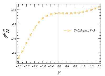
Figure 6: Fluxes $\mathcal{\hat{F}}^{\infty}_{22}$ for the $\ell=m=2$ modes as a function of $\sigma$ for $\hat{a}=0.9$, prograde orbits and $\hat{r}=3$. Notice the nonlinear dependence of the fluxes on $\sigma$ for the extreme case $q=1$.

C.2 Comparison with Akcay et al.

Recently, a new flux balance law relating the local changes of energy of a spinning particle in Kerr spacetime with the asymptotic fluxes of energy and angular momentum was obtained in Ref. Akcay:2019bvk . This procedure has been applied to particles with spin perpendicular to the orbital plane on circular orbits in the Schwarzschild spacetime, computing the linear spin corrections to the fluxes. Table 6 provides our spin corrections to the flux and the fractional difference with respect to the sum of the spin’s contributions at horizon and infinity given in Table I of Ref. Akcay:2019bvk . The errors show a very good agreement between the two results.

$$\begin{array}[]{*{3}{c}}\hline\cr\hline\cr\hat{r}&\delta\mathcal{F}^{\sigma}&\Delta^{\text{rel}}(\delta\mathcal{F}^{\sigma})\\ \hline\cr 10&-1.35324081460517\times 10^{-5}&3.0\times 10^{-14}\\ 8&-6.28540371972\times 10^{-5}&1.9\times 10^{-13}\\ 6&-5.074933017\times 10^{-4}&2.5\times 10^{-11}\\ \hline\cr\hline\cr\hline\cr\hline\cr\end{array}$$

Table 6: Linear spin correction to the GW flux $\delta\mathcal{F}^{\sigma}$ and fractional differences $\Delta^{\text{rel}}(\delta\mathcal{F}^{\sigma})$ with respect to the fluxes shown in Table I of Ref. Akcay:2019bvk for $\hat{a}=0$.

C.3 Comparison with Taracchini et al.

Reference Taracchini:2013wfa computed high-precision GW fluxes for nonspinning particles orbiting around Schwarzschild and Kerr BHs solving the Teukolsky equation in the frequency domain. We have checked our code against both their set-up. The relative errors are shown in Tables 7-9 for the values of the GW fluxes computed at the ISCO and at a different orbital separations $\hat{r}$, as a function of the primary spin. Note that in Ref. Taracchini:2013wfa the sum over the harmonic index $\ell$ was truncated at a certain value $\ell_{\text{max}}$ such that the fractional error between the flux at $\ell_{\text{max}}$ and $\ell_{\text{max}}-1$ was less than $10^{-14}$. To achieve this accuracy the required $\ell_{\text{max}}$ is in general very large: at the ISCO, for example, $\ell_{\text{max}}=30$ for $\hat{a}=0$, and $\ell_{\text{max}}=66$ for $\hat{a}=0.99$. In our calculations we fixed $\ell_{\text{max}}=20$. Nonetheless, the agreement between our results and those computed in Ref. Taracchini:2013wfa is extremely good. Even for the fastest spinning BH considered (with $\hat{a}=0.9$), we find a relative difference smaller than $10^{-5}$.

$$\begin{array}[]{c|c|c|c}\hline\cr\hline\cr\hat{a}&\text{ISCO}&\mathcal{F}^{0}&\Delta^{\text{rel}}(\mathcal{F}^{0})\\ \hline\cr 0.1&5.669&1.203797640\times 10^{-3}&8.5\times 10^{-11}\\ 0.3&4.979&2.10037308\times 10^{-3}&1.4\times 10^{-9}\\ 0.5&4.233&4.11717449\times 10^{-3}&6.9\times 10^{-10}\\ 0.8&2.907&1.71190\times 10^{-2}&4.4\times 10^{-7}\\ 0.9&2.321&3.5223\times 10^{-2}&5.4\times 10^{-6}\\ \hline\cr\hline\cr\end{array}$$

Table 7: Fluxes for a nonspinning objects around Kerr BHs $\mathcal{F}^{0}$ at the ISCO and fractional difference $\Delta^{\text{rel}}(\mathcal{F}^{0})$ compared to the results of Ref. Taracchini:2013wfa .

$$\begin{array}[]{c|ll|ll|ll}\lx@intercol\hfil\hfil\lx@intercol&\lx@intercol\hfil\hat{a}=0\hfil\lx@intercol&\lx@intercol\hfil\hat{a}=0.3\hfil\lx@intercol&\lx@intercol\hfil\hat{a}=0.5\hfil\lx@intercol\\ \hline\cr\hline\cr\hat{r}&\mathcal{F}^{0}&\Delta^{\text{rel}}(\mathcal{F}^{0})&\mathcal{F}^{0}&\Delta^{\text{rel}}(\mathcal{F}^{0})&\mathcal{F}^{0}&\Delta^{\text{rel}}(\mathcal{F}^{0})\\ \hline\cr 10&6.15163167846\times 10^{-5}&1.8\times 10^{-13}&5.72185605812\times 10^{-5}&1.1\times 10^{-12}&5.4706016232\times 10^{-5}&3.0\times 10^{-12}\\ 8&1.9610454858336\times 10^{-4}&1.6\times 10^{-14}&1.757401400491\times 10^{-4}&2.4\times 10^{-14}&1.64390512713\times 10^{-4}&7.2\times 10^{-13}\\ 6&9.40339356\times 10^{-4}&3.8\times 10^{-11}&7.7105423521\times 10^{-4}&1.2\times 10^{-11}&6.8651481394\times 10^{-4}&7.1\times 10^{-12}\\ \hline\cr\hline\cr\hline\cr\hline\cr\end{array}$$

Table 8: Same as Table 7 but for generic orbital separation different from the ISCO, and focusing on $\hat{a}=(0,0.3,0.5)$.

$$\begin{array}[]{c|ll|ll}\lx@intercol\hfil\hfil\lx@intercol&\lx@intercol\hfil\hat{a}=0.8\hfil\lx@intercol&\lx@intercol\hfil\hat{a}=0.9\hfil\lx@intercol\\ \hline\cr\hline\cr\hat{r}&\mathcal{F}&\Delta^{\text{rel}}(\mathcal{F})&\mathcal{F}&\Delta^{\text{rel}}(\mathcal{F})\\ \hline\cr 10&5.13763911701\times 10^{-5}&4.3\times 10^{-13}&5.0368602531\times 10^{-5}&1.4\times 10^{-12}\\ 8&1.49973726131\times 10^{-4}&2.6\times 10^{-13}&1.4574909234\times 10^{-4}&9.5\times 10^{-13}\\ 6&5.8851295900\times 10^{-4}&2.7\times 10^{-12}&5.6168859157\times 10^{-4}&1.5\times 10^{-12}\\ 4&3.9084751\times 10^{-3}&2.2\times 10^{-9}&3.53976293\times 10^{-3}&1.4\times 10^{-9}\\ \hline\cr\hline\cr\hline\cr\hline\cr\end{array}$$

Table 9: Fluxes for a non spinning object $\mathcal{F}^{0}$ and fractional difference $\Delta^{\text{rel}}(\mathcal{F}^{0})$ with respect to the fluxes listed in Taracchini:2013wfa for fast rotating BHs with $\hat{a}=(0.8,09)$.

$$\begin{array}[]{c|ll|ll}\lx@intercol\hfil\hfil\lx@intercol&\lx@intercol\hfil\hat{a}=0.990\hfil\lx@intercol&\lx@intercol\hfil\hat{a}=0.995\hfil\lx@intercol\\ \hline\cr\hline\cr\hat{r}&\mathcal{F}&\Delta^{\text{rel}}(\mathcal{F})&\mathcal{F}&\Delta^{\text{rel}}(\mathcal{F})\\ \hline\cr 10&4.9500572776\times 10^{-5}&2.7\times 10^{-12}&4.9453383948\times 10^{-5}&3.4\times 10^{-12}\\ 8&1.4216152170\times 10^{-4}&1.5\times 10^{-11}&1.419678387\times 10^{-4}&1.4\times 10^{-11}\\ 6&5.395577551\times 10^{-4}&6.6\times 10^{-11}&5.38379633\times 10^{-4}&6.6\times 10^{-11}\\ 4&3.26013974\times 10^{-3}&1.3\times 10^{-9}&3.24583765\times 10^{-3}&1.3\times 10^{-9}\\ 2&4.301\times 10^{-2}&1.1\times 10^{-5}&4.221\times 10^{-2}&1.0\times 10^{-5}\\ \text{ISCO}&9.17\times 10^{-2}&5.0\times 10^{-4}&9.5\times 10^{-2}&1.0\times 10^{-3}\\ \hline\cr\hline\cr\hline\cr\hline\cr\end{array}$$

Table 10: Fluxes for a nonspinning object $\mathcal{F}^{0}$ and fractional difference $\Delta^{\text{rel}}(\mathcal{F}^{0})$ with respect to the fluxes listed in BHPToolkit . The ISCO is at $\hat{r}=1.454$ and $\hat{r}=1.341$ for $\hat{a}=0.990$ and $\hat{a}=0.995$ respectively.

C.4 Comparison with Gralla et al.

Finally, we tested our code in the case of a nonspinning secondary and fast spinning primary BHs with $\hat{a}>0.9$. In this case we use the data obtained in Ref. Gralla:2016qfw using the Teukolsky formalism in the frequency domain and assuming $\ell_{\text{max}}=30$ Gralla:2016qfw . The comparison is shown in Table 10 for $\hat{a}=0.99$ and $\hat{a}=0.995$ for orbital radii equal to and larger than the ISCO. The discrepancy between our results and those of Ref. Gralla:2016qfw increases for larger spins and smaller orbital separation. However, in the worst case scenario, the fluxes differ at most by one part over $10^{3}$.

References

- (1) LISA Collaboration, P. Amaro-Seoane et al., “Laser Interferometer Space Antenna,” arXiv:1702.00786 [astro-ph.IM].
- (2) V. Baibhav et al., “Probing the Nature of Black Holes: Deep in the mHz Gravitational-Wave Sky,” arXiv:1908.11390 [astro-ph.HE].
- (3) S. Babak, J. Gair, A. Sesana, E. Barausse, C. F. Sopuerta, C. P. L. Berry, E. Berti, P. Amaro-Seoane, A. Petiteau, and A. Klein, “Science with the space-based interferometer LISA. V: Extreme mass-ratio inspirals,” Phys. Rev. D95 no. 10, (2017) 103012, arXiv:1703.09722 [gr-qc].
- (4) A. J. K. Chua, N. Korsakova, C. J. Moore, J. R. Gair, and S. Babak, “Gaussian processes for the interpolation and marginalization of waveform error in extreme-mass-ratio-inspiral parameter estimation,” Phys. Rev. D101 no. 4, (2020) 044027, arXiv:1912.11543 [astro-ph.IM].
- (5) L. Barack et al., “Black holes, gravitational waves and fundamental physics: a roadmap,” Class. Quant. Grav. 36 no. 14, (2019) 143001, arXiv:1806.05195 [gr-qc].
- (6) E. Barausse et al., “Prospects for Fundamental Physics with LISA,” arXiv:2001.09793 [gr-qc].
- (7) C. F. Sopuerta and N. Yunes, “Extreme and Intermediate-Mass Ratio Inspirals in Dynamical Chern-Simons Modified Gravity,” Phys. Rev. D80 (2009) 064006, arXiv:0904.4501 [gr-qc].
- (8) N. Yunes, P. Pani, and V. Cardoso, “Gravitational Waves from Quasicircular Extreme Mass-Ratio Inspirals as Probes of Scalar-Tensor Theories,” Phys. Rev. D85 (2012) 102003, arXiv:1112.3351 [gr-qc].
- (9) P. Pani, V. Cardoso, and L. Gualtieri, “Gravitational waves from extreme mass-ratio inspirals in Dynamical Chern-Simons gravity,” Phys. Rev. D83 (2011) 104048, arXiv:1104.1183 [gr-qc].
- (10) E. Barausse, N. Yunes, and K. Chamberlain, “Theory-Agnostic Constraints on Black-Hole Dipole Radiation with Multiband Gravitational-Wave Astrophysics,” Phys. Rev. Lett. 116 no. 24, (2016) 241104, arXiv:1603.04075 [gr-qc].
- (11) K. Chamberlain and N. Yunes, “Theoretical Physics Implications of Gravitational Wave Observation with Future Detectors,” Phys. Rev. D96 no. 8, (2017) 084039, arXiv:1704.08268 [gr-qc].
- (12) V. Cardoso, G. Castro, and A. Maselli, “Gravitational waves in massive gravity theories: waveforms, fluxes and constraints from extreme-mass-ratio mergers,” Phys. Rev. Lett. 121 no. 25, (2018) 251103, arXiv:1809.00673 [gr-qc].
- (13) L. Barack and C. Cutler, “Using LISA EMRI sources to test off-Kerr deviations in the geometry of massive black holes,” Phys. Rev. D75 (2007) 042003, arXiv:gr-qc/0612029 [gr-qc].
- (14) P. Pani, E. Berti, V. Cardoso, Y. Chen, and R. Norte, “Gravitational-wave signatures of the absence of an event horizon. II. Extreme mass ratio inspirals in the spacetime of a thin-shell gravastar,” Phys. Rev. D81 (2010) 084011, arXiv:1001.3031 [gr-qc].
- (15) P. Pani and A. Maselli, “Love in Extrema Ratio,” Int. J. Mod. Phys. D28 no. 14, (2019) 1944001, arXiv:1905.03947 [gr-qc].
- (16) S. Datta, R. Brito, S. Bose, P. Pani, and S. A. Hughes, “Tidal heating as a discriminator for horizons in extreme mass ratio inspirals,” Phys. Rev. D101 no. 4, (2020) 044004, arXiv:1910.07841 [gr-qc].
- (17) A. Pound, “Motion of small objects in curved spacetimes: An introduction to gravitational self-force,” Fund. Theor. Phys. 179 (2015) 399–486, arXiv:1506.06245 [gr-qc].
- (18) L. Barack and A. Pound, “Self-force and radiation reaction in general relativity,” Rept. Prog. Phys. 82 no. 1, (2019) 016904, arXiv:1805.10385 [gr-qc].
- (19) S. R. Dolan, N. Warburton, A. I. Harte, A. Le Tiec, B. Wardell, and L. Barack, “Gravitational self-torque and spin precession in compact binaries,” Phys. Rev. D89 no. 6, (2014) 064011, arXiv:1312.0775 [gr-qc].
- (20) L. M. Burko and G. Khanna, “Self-force gravitational waveforms for extreme and intermediate mass ratio inspirals. III: Spin-orbit coupling revisited,” Phys. Rev. D91 no. 10, (2015) 104017, arXiv:1503.05097 [gr-qc].
- (21) N. Warburton, T. Osburn, and C. R. Evans, “Evolution of small-mass-ratio binaries with a spinning secondary,” Phys. Rev. D96 no. 8, (2017) 084057, arXiv:1708.03720 [gr-qc].
- (22) S. Akcay, S. R. Dolan, C. Kavanagh, J. Moxon, N. Warburton, and B. Wardell, “Dissipation in extreme-mass ratio binaries with a spinning secondary,” arXiv:1912.09461 [gr-qc].
- (23) Y. Mino, M. Shibata, and T. Tanaka, “Gravitational waves induced by a spinning particle falling into a rotating black hole,” Phys. Rev. D53 (1996) 622–634. [Erratum: Phys. Rev.D59,047502(1999)].
- (24) M. Saijo, K.-i. Maeda, M. Shibata, and Y. Mino, “Gravitational waves from a spinning particle plunging into a Kerr black hole,” Phys. Rev. D58 (1998) 064005.
- (25) K. Tominaga, M. Saijo, and K.-i. Maeda, “Gravitational waves from a spinning particle scattered by a relativistic star: Axial mode case,” Phys. Rev. D63 (2001) 124012, arXiv:gr-qc/0009055 [gr-qc].
- (26) T. Tanaka, Y. Mino, M. Sasaki, and M. Shibata, “Gravitational waves from a spinning particle in circular orbits around a rotating black hole,” Phys. Rev. D54 (1996) 3762–3777, arXiv:gr-qc/9602038 [gr-qc].
- (27) A. Nagar, F. Messina, C. Kavanagh, G. Lukes-Gerakopoulos, N. Warburton, S. Bernuzzi, and E. Harms, “Factorization and resummation: A new paradigm to improve gravitational wave amplitudes. III: the spinning test-body terms,” Phys. Rev. D100 no. 10, (2019) 104056, arXiv:1907.12233 [gr-qc].
- (28) L. M. Burko, “Orbital evolution of a particle around a black hole. 2. Comparison of contributions of spin orbit coupling and the selfforce,” Phys. Rev. D 69 (2004) 044011, arXiv:gr-qc/0308003.
- (29) E. Harms, G. Lukes-Gerakopoulos, S. Bernuzzi, and A. Nagar, “Asymptotic gravitational wave fluxes from a spinning particle in circular equatorial orbits around a rotating black hole,” Phys. Rev. D93 no. 4, (2016) 044015, arXiv:1510.05548 [gr-qc]. [Addendum: Phys. Rev.D100,no.12,129901(2019)].
- (30) E. Harms, G. Lukes-Gerakopoulos, S. Bernuzzi, and A. Nagar, “Spinning test body orbiting around a Schwarzschild black hole: Circular dynamics and gravitational-wave fluxes,” Phys. Rev. D94 no. 10, (2016) 104010, arXiv:1609.00356 [gr-qc].
- (31) G. Lukes-Gerakopoulos, E. Harms, S. Bernuzzi, and A. Nagar, “Spinning test-body orbiting around a Kerr black hole: circular dynamics and gravitational-wave fluxes,” Phys. Rev. D96 no. 6, (2017) 064051, arXiv:1707.07537 [gr-qc].
- (32) N. Yunes, A. Buonanno, S. A. Hughes, Y. Pan, E. Barausse, M. Miller, and W. Throwe, “Extreme Mass-Ratio Inspirals in the Effective-One-Body Approach: Quasi-Circular, Equatorial Orbits around a Spinning Black Hole,” Phys. Rev. D 83 (2011) 044044, arXiv:1009.6013 [gr-qc]. [Erratum: Phys.Rev.D 88, 109904 (2013)].
- (33) B. Chen, G. Compère, Y. Liu, J. Long, and X. Zhang, “Spin and Quadrupole Couplings for High Spin Equatorial Intermediate Mass-ratio Coalescences,” Class. Quant. Grav. 36 no. 24, (2019) 245011, arXiv:1901.05370 [gr-qc].
- (34) G. A. Piovano, A. Maselli, and P. Pani, “Model independent tests of the Kerr bound with extreme mass ratio inspirals,” arXiv:2003.08448 [gr-qc].
- (35) “xAct: Efficient tensor computer algebra for the Wolfram Language.” (xact.es).
- (36) W. Tulczyjew, “Motion of multipole particles in general relativity theory,” Acta Phys. Pol. 18 (1959) 393.
- (37) W. Dixon, “A covariant multipole formalism for extended test bodies in general relativity,” Il Nuovo Cimento 34 no. 2, (Oct, 1964) 317–339.
- (38) W. G. Dixon, “Dynamics of extended bodies in general relativity. I. Momentum and angular momentum,” Proc. Roy. Soc. Lond. A314 (1970) 499–527.
- (39) W. G. Dixon, “Dynamics of extended bodies in general relativity. II. Moments of the charge-current vector,” Proc. Roy. Soc. Lond. A319 (1970) 509–547.
- (40) K. Kyrian and O. Semerak, “Spinning test particles in a Kerr field,” Mon. Not. Roy. Astron. Soc. 382 (2007) 1922.
- (41) W. Dixon, “Extended bodies in general relativity; their description and motion,” in Isolated Gravitating Systems in General Relativity - Proceedings of the International School of Physics ”Enrico Fermi”. 1978.
- (42) M. Mathisson, “Neue mechanik materieller systemes,” Acta Phys. Polon. 6 (1937) 163–2900.
- (43) A. Papapetrou, “Spinning test particles in general relativity. 1.,” Proc. Roy. Soc. Lond. A209 (1951) 248–258.
- (44) E. Corinaldesi and A. Papapetrou, “Spinning test particles in general relativity. 2.,” Proc. Roy. Soc. Lond. A209 (1951) 259–268.
- (45) J. Steinhoff and D. Puetzfeld, “Multipolar equations of motion for extended test bodies in General Relativity,” Phys. Rev. D81 (2010) 044019, arXiv:0909.3756 [gr-qc].
- (46) O. Semerak, “Spinning test particles in a Kerr field. 1.,” Mon. Not. Roy. Astron. Soc. 308 (1999) 863–875.
- (47) F. Costa, C. A. R. Herdeiro, J. Natario, and M. Zilhao, “Mathisson’s helical motions for a spinning particle: Are they unphysical?,” Phys. Rev. D85 (2012) 024001, arXiv:1109.1019 [gr-qc].
- (48) L. F. O. Costa and J. Natário, “Center of mass, spin supplementary conditions, and the momentum of spinning particles,” Fund. Theor. Phys. 179 (2015) 215–258, arXiv:1410.6443 [gr-qc].
- (49) J. Ehlers and E. Rudolph, “Dynamics of extended bodies in general relativity center-of-mass description and quasirigidity,” General Relativity and Gravitation 8 no. 3, (Mar, 1977) 197–217.
- (50) G. Lukes-Gerakopoulos, “Time parameterizations and spin supplementary conditions of the Mathisson-Papapetrou-Dixon equations,” Phys. Rev. D96 no. 10, (2017) 104023, arXiv:1709.08942 [gr-qc].
- (51) V. Witzany, J. Steinhoff, and G. Lukes-Gerakopoulos, “Hamiltonians and canonical coordinates for spinning particles in curved space-time,” Class. Quant. Grav. 36 no. 7, (2019) 075003, arXiv:1808.06582 [gr-qc].
- (52) C. Møl̃ler, “Sur la dynamique des systèmes ayant un moment angulaire interne,” Annales de l’institut Henri Poincaré 11 no. 5, (1949) 251–278. http://eudml.org/doc/79030.
- (53) J. Steinhoff and D. Puetzfeld, “Influence of internal structure on the motion of test bodies in extreme mass ratio situations,” Phys. Rev. D86 (2012) 044033, arXiv:1205.3926 [gr-qc].
- (54) P. I. Jefremov, O. Yu. Tsupko, and G. S. Bisnovatyi-Kogan, “Innermost stable circular orbits of spinning test particles in Schwarzschild and Kerr space-times,” Phys. Rev. D91 no. 12, (2015) 124030, arXiv:1503.07060 [gr-qc].
- (55) S. Suzuki and K.-i. Maeda, “Innermost stable circular orbit of a spinning particle in Kerr space-time,” Phys. Rev. D58 (1998) 023005, arXiv:gr-qc/9712095 [gr-qc].
- (56) J. M. Bardeen, W. H. Press, and S. A. Teukolsky, “Rotating Black Holes: Locally Nonrotating Frames, Energy Extraction, and Scalar Synchrotron Radiation,” The Astrophysical Journal 178 (Dec, 1972) 347–370.
- (57) T. Hinderer and E. E. Flanagan, “Two timescale analysis of extreme mass ratio inspirals in Kerr. I. Orbital Motion,” Phys. Rev. D78 (2008) 064028, arXiv:0805.3337 [gr-qc].
- (58) S. A. Hughes, “Bound orbits of a slowly evolving black hole,” Phys. Rev. D100 no. 6, (2019) 064001, arXiv:1806.09022 [gr-qc].
- (59) A. Ori and K. S. Thorne, “The Transition from inspiral to plunge for a compact body in a circular equatorial orbit around a massive, spinning black hole,” Phys. Rev. D 62 (2000) 124022, arXiv:gr-qc/0003032.
- (60) O. Burke, J. R. Gair, and J. Simón, “Transition from Inspiral to Plunge: A Complete Near-Extremal Trajectory and Associated Waveform,” Phys. Rev. D 101 no. 6, (2020) 064026, arXiv:1909.12846 [gr-qc].
- (61) G. Compère, K. Fransen, and C. Jonas, “Transition from inspiral to plunge into a highly spinning black hole,” Class. Quant. Grav. 37 no. 9, (2020) 095013, arXiv:1909.12848 [gr-qc].
- (62) D. Kennefick, “Stability under radiation reaction of circular equatorial orbits around Kerr black holes,” Phys. Rev. D 58 (1998) 064012, arXiv:gr-qc/9805102.
- (63) D. Kennefick and A. Ori, “Radiation reaction induced evolution of circular orbits of particles around Kerr black holes,” Phys. Rev. D 53 (1996) 4319–4326, arXiv:gr-qc/9512018.
- (64) “Black Hole Perturbation Toolkit.” (bhptoolkit.org).
- (65) Y. Mino, M. Sasaki, M. Shibata, H. Tagoshi, and T. Tanaka, “Black hole perturbation: Chapter 1,” Prog. Theor. Phys. Suppl. 128 (1997) 1–121, arXiv:gr-qc/9712057 [gr-qc].
- (66) S. Mano, H. Suzuki, and E. Takasugi, “Analytic solutions of the Teukolsky equation and their low frequency expansions,” Prog. Theor. Phys. 95 (1996) 1079–1096, arXiv:gr-qc/9603020 [gr-qc].
- (67) R. Fujita and H. Tagoshi, “New numerical methods to evaluate homogeneous solutions of the Teukolsky equation,” Prog. Theor. Phys. 112 (2004) 415–450, arXiv:gr-qc/0410018 [gr-qc].
- (68) R. Fujita, W. Hikida, and H. Tagoshi, “An Efficient Numerical Method for Computing Gravitational Waves Induced by a Particle Moving on Eccentric Inclined Orbits around a Kerr Black Hole,” Prog. Theor. Phys. 121 (2009) 843–874, arXiv:0904.3810 [gr-qc].
- (69) S. A. Hughes, “The Evolution of circular, nonequatorial orbits of Kerr black holes due to gravitational wave emission,” Phys. Rev. D61 no. 8, (2000) 084004, arXiv:gr-qc/9910091 [gr-qc]. [Erratum: Phys. Rev.D63,no.4,049902(2001); Erratum: Phys. Rev.D65,no.6,069902(2002); Erratum: Phys. Rev.D67,no.8,089901(2003); Erratum: Phys. Rev.D78,no.10,109902(2008); Erratum: Phys. Rev.D90,no.10,109904(2014)].
- (70) Data and relevant codes are publicly available at https://web.uniroma1.it/gmunu.
- (71) S. E. Gralla, S. A. Hughes, and N. Warburton, “Inspiral into Gargantua,” Class. Quant. Grav. 33 no. 15, (2016) 155002, arXiv:1603.01221 [gr-qc].
- (72) E. Huerta and J. R. Gair, “Importance of including small body spin effects in the modelling of extreme and intermediate mass-ratio inspirals,” Phys. Rev. D 84 (2011) 064023, arXiv:1105.3567 [gr-qc].
- (73) LISA Data Challenge Working Group. LISA Data Challenges, 2019. https://lisa-ldc.lal.in2p3.fr.
- (74) L. Lindblom, B. J. Owen, and D. A. Brown, “Model Waveform Accuracy Standards for Gravitational Wave Data Analysis,” Phys. Rev. D78 (2008) 124020, arXiv:0809.3844 [gr-qc].
- (75) E. E. Flanagan and S. A. Hughes, “Measuring gravitational waves from binary black hole coalescences: 2. The Waves’ information and its extraction, with and without templates,” Phys. Rev. D57 (1998) 4566–4587, arXiv:gr-qc/9710129 [gr-qc].
- (76) M. D. Hartl, “Dynamics of spinning test particles in Kerr space-time,” Phys. Rev. D67 (2003) 024005, arXiv:gr-qc/0210042 [gr-qc].
- (77) E. G. Gimon and P. Horava, “Astrophysical violations of the Kerr bound as a possible signature of string theory,” Phys. Lett. B672 (2009) 299–302, arXiv:0706.2873 [hep-th].
- (78) P. Pani, E. Barausse, E. Berti, and V. Cardoso, “Gravitational instabilities of superspinars,” Phys. Rev. D82 (2010) 044009, arXiv:1006.1863 [gr-qc].
- (79) E. Maggio, P. Pani, and V. Ferrari, “Exotic Compact Objects and How to Quench their Ergoregion Instability,” Phys. Rev. D96 no. 10, (2017) 104047, arXiv:1703.03696 [gr-qc].
- (80) E. Maggio, V. Cardoso, S. R. Dolan, and P. Pani, “Ergoregion instability of exotic compact objects: electromagnetic and gravitational perturbations and the role of absorption,” Phys. Rev. D 99 no. 6, (2019) 064007, arXiv:1807.08840 [gr-qc].
- (81) R. Roy, P. Kocherlakota, and P. S. Joshi, “Mode stability of a near-extremal Kerr superspinar,” arXiv:1911.06169 [gr-qc].
- (82) B. C. Bisscheroux, O. R. Pols, P. Kahabka, T. Belloni, and E. P. J. van den Heuvel, “The nature of the bright subdwarf HD 49798 and its X-ray pulsating companion.,” A&A 317 (Feb., 1997) 815–822.
- (83) J. W. Hessels, S. M. Ransom, I. H. Stairs, P. C. C. Freire, V. M. Kaspi, and F. Camilo, “A radio pulsar spinning at 716-hz,” Science 311 (2006) 1901–1904, arXiv:astro-ph/0601337.
- (84) R. N. Manchester, G. B. Hobbs, A. Teoh, and M. Hobbs, “The Australia Telescope National Facility pulsar catalogue,” Astron. J. 129 (2005) 1993, arXiv:astro-ph/0412641.
- (85) V. Cardoso and P. Pani, “Testing the nature of dark compact objects: a status report,” Living Rev. Rel. 22 no. 1, (2019) 4, arXiv:1904.05363 [gr-qc].
- (86) E. Berti et al., “Testing General Relativity with Present and Future Astrophysical Observations,” Class. Quant. Grav. 32 (2015) 243001, arXiv:1501.07274 [gr-qc].
- (87) E. Barausse, V. Cardoso, and P. Pani, “Can environmental effects spoil precision gravitational-wave astrophysics?,” Phys. Rev. D 89 no. 10, (2014) 104059, arXiv:1404.7149 [gr-qc].
- (88) A. Maselli, N. Franchini, L. Gualtieri, and T. P. Sotiriou, “Detecting scalar fields with Extreme Mass Ratio Inspirals,” arXiv:2004.11895 [gr-qc].
- (89) V. Witzany, “Hamilton-Jacobi equation for spinning particles near black holes,” Phys. Rev. D100 no. 10, (2019) 104030, arXiv:1903.03651 [gr-qc].
- (90) D. Bini, A. Geralico, R. T. Jantzen, and F. de Felice, “Spin precession along circular orbits in the Kerr spacetime: the Frenet-Serret description,” Class. Quant. Grav. 23 (2006) 3287–3304, arXiv:1408.4278 [gr-qc].
- (91) U. Ruangsri, S. J. Vigeland, and S. A. Hughes, “Gyroscopes orbiting black holes: A frequency-domain approach to precession and spin-curvature coupling for spinning bodies on generic Kerr orbits,” Phys. Rev. D94 no. 4, (2016) 044008, arXiv:1512.00376 [gr-qc].
- (92) T. Hinderer et al., “Periastron advance in spinning black hole binaries: comparing effective-one-body and Numerical Relativity,” Phys. Rev. D88 no. 8, (2013) 084005, arXiv:1309.0544 [gr-qc].
- (93) D. Bini and A. Geralico, “Extended bodies in a Kerr spacetime: exploring the role of a general quadrupole tensor,” Class. Quant. Grav. 31 (2014) 075024, arXiv:1408.5484 [gr-qc].
- (94) O. Zelenka, G. Lukes-Gerakopoulos, V. Witzany, and O. Kopác̆ek, “Growth of resonances and chaos for a spinning test particle in the Schwarzschild background,” Phys. Rev. D101 no. 2, (2020) 024037, arXiv:1911.00414 [gr-qc].
- (95) G. Lukes-Gerakopoulos, “Spinning particles moving around black holes: integrability and chaos,” in Proceedings, 14th Marcel Grossmann Meeting on Recent Developments in Theoretical and Experimental General Relativity, Astrophysics, and Relativistic Field Theories (MG14) (In 4 Volumes): Rome, Italy, July 12-18, 2015, vol. 2, pp. 1960–1965. 2017. arXiv:1606.09430 [gr-qc].
- (96) M. Sasaki and T. Nakamura, “Gravitational Radiation From a Kerr Black Hole. 1. Formulation and a Method for Numerical Analysis,” Prog. Theor. Phys. 67 (1982) 1788.
- (97) F. W. J. Olver, “Asymptotic expansions of the coefficients in asymptotic series solutions of linear differential equations,” Methods Appl. Anal. 1 no. 1, (1994) 1–13.
- (98) F. W. J. Olver, “Asymptotic solutions of linear ordinary differential equations at an irregular singularity of rank unity,” Methods Appl. Anal. 4 no. 4, (1997) 375–403.
- (99) F. Olver, Asymptotics and Special Functions. Computer science and applied mathematics : a series of monographs and textbooks. Academic Press, 1974.
- (100) S. E. Gralla, A. P. Porfyriadis, and N. Warburton, “Particle on the Innermost Stable Circular Orbit of a Rapidly Spinning Black Hole,” Phys. Rev. D92 no. 6, (2015) 064029, arXiv:1506.08496 [gr-qc].
- (101) A. Taracchini, A. Buonanno, S. A. Hughes, and G. Khanna, “Modeling the horizon-absorbed gravitational flux for equatorial-circular orbits in Kerr spacetime,” Phys. Rev. D88 (2013) 044001, arXiv:1305.2184 [gr-qc]. [Erratum: Phys. Rev.D88,no.10,109903(2013)].