Efficient Alternating Least Squares Algorithms for Low Multilinear Rank Approximation of Tensors

Abstract

The low multilinear rank approximation, also known as the truncated Tucker decomposition, has been extensively utilized in many applications that involve higher-order tensors. Popular methods for low multilinear rank approximation usually rely directly on matrix SVD, therefore often suffer from the notorious intermediate data explosion issue and are not easy to parallelize, especially when the input tensor is large. In this paper, we propose a new class of truncated HOSVD algorithms based on alternating least squares (ALS) for efficiently computing the low multilinear rank approximation of tensors. The proposed ALS-based approaches are able to eliminate the redundant computations of the singular vectors of intermediate matrices and are therefore free of data explosion. Also, the new methods are more flexible with adjustable convergence tolerance and are intrinsically parallelizable on high-performance computers. Theoretical analysis reveals that the ALS iteration in the proposed algorithms is q-linear convergent with a relatively wide convergence region. Numerical experiments with large-scale tensors from both synthetic and real-world applications demonstrate that ALS-based methods can substantially reduce the total cost of the original ones and are highly scalable for parallel computing.

1 Introduction

As a natural extension of vectors (first-order) and matrices (second-order), higher-order tensors have been receiving increasingly more attention in various applications, such as signal processing Lathauwer2004 ; Sidiropoulos2017 , computer vision Shashua2001 ; Vasilescu2002 ; Vlasi2005 , chemometrics Henrion1993 ; Jiang2000 ; Bro2006 , deep learning Charalampous2014 ; Novikov2015 , and scientific computing Beylkin2002 ; Khoromskij2012 ; Hackbusch2014 . For decades, tensor decompositions have been extensively utilized as an efficient tool for dimension reductions, latent variable analysis and other purposes in a wide range of scientific and engineering fields Hackbusch2014 ; Beckmann2005 ; Kroonenberg2008 ; Ishteva2008 ; Holtz2012 ; Ding2016 . There exist a number of tensor decomposition models, such as canonical polyadic (CP, or CANDECOMP/PARAFAC) decomposition Hitchcock1927 ; Carroll1970 ; Kiers2000 , Tucker decomposition Tucker1966 ; Levin1963 ; Lathauwer2000-1 , tensor train (TT) model Oseledets2011 , and hierarchical Tucker (HT) model Grasedyck2010 ; Hackbusch2009 ; Oseledets2009 . Among them, the Tucker decomposition, also known as the higher-order singular value decomposition (HOSVD), is regarded as a generalization of the matrix singular value decomposition (SVD) and has been applied with significant successes in many applications Tucker1966 ; Levin1963 ; Lathauwer2000-1 ; Lathauwer2004 ; Ishteva2008 ; Kolda2009 .

In both theory and practice, a commonly considered tensor computation problem is the low multilinear rank approximation Lathauwer2000-2 ; Kolda2009 , also known as the truncated Tucker decomposition Vannieuwenhoven2012 ; Austin2016 , which reads

$$\min_{\bm{\mathcal{B}}}\|\bm{\mathcal{A}}-\bm{\mathcal{B}}\|,$$ (1.1)

where $\bm{\mathcal{A}}\in\mathbb{R}^{I_{1}\times I_{2}\times\cdots\times I_{N}}$ is a given $N$th-order tensor and $\bm{\mathcal{B}}\in\mathbb{R}^{I_{1}\times I_{2}\times\cdots\times I_{N}}$ is its low multilinear rank approximation Lathauwer2000-1 ; Kolda2009 . Existing approaches for solving (1.1) can be roughly divided into two categories Vannieuwenhoven2011 : non-iterative and iterative methods. The most popular non-iterative algorithms for the low multilinear rank approximation of higher-order tensors is the truncated HOSVD ($t$-HOSVD) Tucker1966 ; Lathauwer2000-2 and its improved version, the sequentially truncated HOSVD ($st$-HOSVD) Vannieuwenhoven2012 . Despite the fact that the results of $t$-HOSVD and $st$-HOSVD are usually suboptimal, they can serve as good initial solution for popular iterative methods such as higher-order orthogonal iteration (HOOI) Kroonenberg1980 ; Lathauwer2000-2 . Other than the HOOI method, which is a first-order iterative method, some efforts are also made in developing second-order approaches, such as Newton-type Elden2009 ; Savas2010 ; Ishteva2009 and trust-region Ishteva2008 ; Ishteva2011 algorithms. Although these methods can achieve faster convergence under certain conditions, they are still in early study and are usually not suitable for large-scale tensors Xu2018 .

In this paper, we focus on studying how to efficiently compute the truncated Tucker decomposition (1.1) of higher-order tensors by modifying the $t$-HOSVD and $st$-HOSVD algorithms so that certain fast iterative procedures are included. As a major cost of the two algorithms, the computation of tensor-matrix multiplications has been extensively optimized in a number of high-performance tensor libraries Rajbhandari2014 ; Li2015 ; Smith2015 ; Schatz2015 , and therefore is not the focus of this study. Another potential bottleneck of the $t$-HOSVD and $st$-HOSVD algorithms is the calculation of the singular vectors of the intermediate matrices, which can be done by applying SVD to the matricized tensor or eigen-decomposition to the Gram matrix Kroonenberg1980 ; Lathauwer2000-2 ; Kolda2009 ; Austin2016 ; Oh2017 . The matrix SVD can be obtained by using Krylov subspace methods Golub2008 ; Culum1983 ; Baglama2005 , whilst the eigen-decomposition of the symmeric nonnegative definite Gram matrix can be done with a Krylov-Schur algorithm Sorensen1992 ; Stewart2001 ; Watkins2008 ; Golub2008 . Due to the fact that these methods rely on the factorization of intermediate matrices, they suffer from the notorious data explosion issue Austin2016 ; Oh2017 ; Oh2019 . And even if the hardware storage allowed, they are still not scalable for parallel computing and the total computation cost could be unbearably high.

In order to improve the performance of the $t$-HOSVD and $st$-HOSVD algorithms, we propose a class of alternating least squares (ALS) based algorithms for efficiently calculating the low multilinear rank approximation of tensors. The key observation is that in the original algorithms the computations of singular vectors of the intermediate matrices are indeed not necessary and can be replaced with low rank approximations, and the low rank approximations can be done by using an ALS method which does not explicitly require intermediate tensor matricization, with the help of a row-wise update rule. The proposed ALS-based algorithms enjoy advantages in computing efficiency, error adaptivity and parallel scalability, especially for large-scale tensors. We present theoretical analysis and show that the ALS iteration in the proposed algorithms is q-linear convergent with a relatively wide convergence region. Several numerical experiments with both synthetic and real-world tensor data demonstrate that new algorithms can effectively alleviate the data explosion issue of the original ones and are highly parallelizable on parallel computers.

The organization of the paper is as follows. In Sec. 2, we introduce some basic notations of tensor and the corresponding algorithms. In Sec. 3, the $t$-HOSVD-ALS and $st$-HOSVD-ALS algorithms are proposed. Some theoretical analysis on the convergence behavior of the ALS methods can also be found in Sec. 3. After that, computational complexity and the approximation errors of proposed algorithms are analyzed in Sec. 4. Test results on several numerical experiments are reported in Sec. 5. And the paper is concluded in Sec. 6.

2 Notations and Nomenclatures

Symbols frequently used in this paper can be found in the following table.

Symbols	Notations
$a$	scalar
$\bm{a}$	vector
$\bm{A}$	matrix
$\bm{\mathcal{A}}$	three or higher-order tensor
$\circ$	vector outer product
$\times_{n}$	mode-$n$ product of tensor and matrix
$\bm{I}_{n}$	identity matrix with size $n\times n$
$I_{n:N}$	$\prod\limits_{i=n}^{N}I_{i}$
$\mathcal{R}(\bm{A})$	a subspace formed by the columns of matrix $\bm{A}$
$\sigma(\bm{A})$	a set that consists of sigular values of matrix $\bm{A}$
$\bm{A}^{\dagger}$	pseudo-inverse of matrix $\bm{A}$

Given an $N$th-order tensor $\bm{\mathcal{A}}\in\mathbb{R}^{I_{1}\times I_{2}\times\cdots\times I_{N}}$, we denote $\bm{\mathcal{A}}_{i_{1},i_{2},\cdots,i_{N}}$ as its $(i_{1},i_{2},\cdots,i_{N})$-th element. In particular, rank one tensor is denoted as

$$\bm{u}_{1}\circ\bm{u}_{2}\circ\cdots\circ\bm{u}_{N},$$

where $\bm{u}_{n}\in\mathbb{R}^{I_{n}}$ is a vector.

The Frobenius norm of tensor $\bm{\mathcal{A}}$ is defined as

$$\|\bm{\mathcal{A}}\|_{F}=\sqrt{\sum\limits_{i_{1},i_{2},\cdots,i_{N}}\bm{\mathcal{A}}_{i_{1},i_{2},\cdots,i_{N}}^{2}}.$$

The matricization of a higher-order tensor is a process of reordering the elements of the tensor into a matrix. For example, the mode-$n$ matricization of tensor $\bm{\mathcal{A}}$ is denoted as $\bm{A}_{(n)}$, which is a matrix belonging to $\mathbb{R}^{I_{n}\times(I_{1}\cdots I_{n-1}I_{n+1}\cdots I_{N})}$. Specifically, the $(i_{1},i_{2},\cdots,i_{N})$-th element of tensor $\bm{\mathcal{A}}$ is mapped to the $(i_{n},j)$-th entry of matrix $\bm{A}_{(n)}$, where

$$j=1+\sum\limits_{k=1,k\neq n}^{N}(i_{k}-1)J_{k}\ \ \mbox{with}\ \ J_{k}=\prod\limits_{m=1,m\neq n}^{k-1}I_{m}.$$

The multilinear rank of a higher-order tensor $\bm{\mathcal{A}}$ is an integer array $(R_{1},R_{2},\cdots,R_{N})$, where $R_{n}$ is the rank of its mode-$n$ matricization $\bm{A}_{(n)}$.

A frequently encountered operation in tensor computation is the tensor-matrix multiplication. In particular, the mode-$n$ tensor-matrix multiplication refers to the contraction of the tensor with a matrix along the $n$-th index. For example, suppose that $\bm{U}\in\mathbb{R}^{J\times I_{n}}$ is a matrix, the mode-$n$ product of $\bm{\mathcal{A}}$ and $\bm{U}$ is denoted as $\bm{\mathcal{A}}\times_{n}\bm{U}\in\mathbb{R}^{I_{1}\times\cdots\times I_{n-1}\times J\times I_{n+1}\times\cdots\ I_{N}}$. Elementwisely, one has

$$\bm{\mathcal{B}}_{i_{1},\cdots,j,\cdots,i_{N}}=(\bm{\mathcal{A}}\times_{n}\bm{U})_{i_{1},\cdots,j,\cdots,i_{N}}=\sum\limits_{i_{n}=1}^{I_{n}}\bm{\mathcal{A}}_{i_{1},\cdots,i_{n},\cdots,i_{N}}\bm{U}_{j,i_{n}}.$$

The Tucker decomposition Tucker1966 ; Levin1963 , also known as the higher-order singular value decomposition (HOSVD) Lathauwer2000-1 , is formally defined as

$$\bm{\mathcal{A}}=\bm{\mathcal{G}}\times_{1}\bm{U}^{(1)}\times_{2}\bm{U}^{(2)}\cdots\times_{N}\bm{U}^{(N)},$$

where $\bm{\mathcal{G}}\in\mathbb{R}^{R_{1}\times R_{2}\times\cdots\times R_{N}}$ is referred to as the core tensor and $\bm{U}^{(n)}\in\mathbb{R}^{I_{n}\times R_{n}}$ are column orthogonal with each other for all $n\in\{1,2,\cdots,N\}$. We remark here that the size of the core tensor is often smaller than that of the original tensor, though it is hard to know how small it can be a prior Silva2008 ; Kolda2009 . In many applications, the Tucker decomposition is usually applied in its truncated form, which reads

$$\begin{split}\min\limits_{\bm{\mathcal{G}};\bm{U}^{(1)},\bm{U}^{(2)},\cdots,\bm{U}^{(N)}}\|\bm{\mathcal{A}}-\bm{\mathcal{G}}\times_{1}\bm{U}^{(1)}\times_{2}\bm{U}^{(2)}\cdots\times_{N}\bm{U}^{(N)}\|,\\ s.t.\ \ \ \ \bm{U}^{(n)T}\bm{U}^{(n)}=\bm{I}_{R_{n}},\ n\in\{1,2,\cdots,N\}\end{split}$$ (2.1)

where $(R_{1},R_{2},\cdots,R_{N})$ is a pre-determined truncation, smaller than the size of original tensor. Suppose that the exact solution of (2.1) is $\bm{U}^{*(1)}$, $\bm{U}^{*(2)}$, $\cdots$, $\bm{U}^{*(N)}$, and $\bm{\mathcal{G}}^{*}$, then it is easy to see that

$$\bm{\mathcal{G}}^{*}=\bm{\mathcal{A}}\times_{1}(\bm{U}^{*(1)})^{T}\times_{2}(\bm{U}^{*(2)})^{T}\cdots\times_{N}(\bm{U}^{*(N)})^{T},$$

which means

$$\bm{\mathcal{A}}\times_{1}(\bm{U}^{*(1)})(\bm{U}^{*(1)})^{T}\times_{2}(\bm{U}^{*(2)})(\bm{U}^{*(2)})^{T}\cdots\times_{N}(\bm{U}^{*(N)})(\bm{U}^{*(N)})^{T}$$ (2.2)

is the best low multilinear rank approximation of $\bm{\mathcal{A}}$.

To compute the best low multilinear rank approximation of a higher-order tensor in the truncated Tucker decomposition, a popular approach is the truncated HOSVD ($t$-HOSVD, Tucker1966 ) originally presented by Tucker himself Tucker1966 . Nowadays, it is better known with the effort of Lathauwer et al. Lathauwer2000-2 , who analyzed the structure of core tensor and proposed to employ SVD of the intermediate matrices in truncated HOSVD. The computing procedure of $t$-HOSVD is given in Algorithm 1.

Algorithm 1 $t$-HOSVD Tucker1966 ; Lathauwer2000-2

0:  Tensor $\bm{\mathcal{A}}\in\mathbb{R}^{I_{1}\times I_{2}\times\cdots\times I_{N}}$, truncation $(R_{1},R_{2},\cdots,R_{N})$

0:  Low multilinear rank approximation $\hat{\bm{\mathcal{A}}}\approx\bm{\mathcal{G}}\times_{1}\bm{U}^{(1)}\times_{2}\bm{U}^{(2)}\cdots\times_{N}\bm{U}^{(N)}$

1:  for all $n\in\{1,2,\cdots,N\}$ do

2:     $\bm{Q}\leftarrow$ leading left singular vectors of $\bm{A}_{(n)}$

3:     $\bm{U}^{(n)}\leftarrow\bm{Q}$

4:  end for

5:  $\bm{\mathcal{G}}\leftarrow\bm{\mathcal{A}}\times_{1}\bm{U}^{(1)T}\times_{2}\bm{U}^{(2)T}\cdots\times_{N}\bm{U}^{(N)T}$

We remark here that in Algorithm 1, the computation of $\bm{Q}$ can also be done by calculating the $R_{n}$ eigenvectors of the Gram matrix $\bm{A}_{(n)}\bm{A}_{(n)}^{T}$. It is clear that $t$-HOSVD can be seen as a natural extension of the truncated SVD of a matrix to higher-order tensors. But unlike the matrix case, the approximation error of $t$-HOSVD is quasi-optimal Tucker1966 ; Lathauwer2000-2 ; Kolda2009 ; Vannieuwenhoven2012 .

As a subsequent improvement of $t$-HOSVD, the sequentially truncated HOSVD ($st$-HOSVD), proposed by Vannieuwenhoven et al. Vannieuwenhoven2012 uses a different truncation strategy, as shown in Algorithm 2.

Algorithm 2 $st$-HOSVD Vannieuwenhoven2012

0:  Tensor $\bm{\mathcal{A}}\in\mathbb{R}^{I_{1}\times I_{2}\times\cdots\times I_{N}}$, truncation $(R_{1},R_{2},\cdots,R_{N})$

0:  Low multilinear rank approximation $\hat{\bm{\mathcal{A}}}\approx\bm{\mathcal{G}}\times_{1}\bm{U}^{(1)}\times_{2}\bm{U}^{(2)}\cdots\times_{N}\bm{U}^{(N)}$

1:  Select an order of $\{1,2,\cdots,N\}$, i.e., $\{i_{1},i_{2},\cdots,i_{N}\}$.

2:  $\bm{\mathcal{B}}\ \leftarrow\ \bm{\mathcal{A}}$

3:  for all $n\in\{i_{1},i_{2},\cdots,i_{N}\}$ do

4:     $\bm{U},\bm{\Sigma},\bm{V}^{T}\ \leftarrow$ matrix SVD of $\bm{B}_{(n)}$

5:     $\bm{U}^{(n)}\ \leftarrow\ \bm{U}$

6:     $\bm{\mathcal{B}}\ \leftarrow\ \bm{\Sigma}\bm{V}^{T}$ in tensor format

7:  end for

8:  $\bm{\mathcal{G}}\ \leftarrow\ \bm{\mathcal{B}}$

Analogous to $t$-HOSVD, in Algorithm 2 one can also obtain $\bm{Q}$ by computing the $R_{n}$ eigenvectors of the Gram matrix $\bm{B}_{(n)}\bm{B}_{(n)}^{T}$, and the core tensor is updated by $\bm{\mathcal{B}}=\bm{\mathcal{B}}\times_{n}\bm{U}^{(n)T}$.

Unlike $t$-HOSVD, the $st$-HOSVD algorithm does not compute the singular vectors of $\bm{A}_{(n)}$. In particular, the factor matrices and core tensor in $st$-HOSVD are calculated simultaneously, which greatly reduces the size of the intermediate matrices. It is worth mentioning that the order of $\{1,2,\cdots,N\}$ in Algorithm 2 could have a strong influence on the computational cost and approximation error of $st$-HOSVD. But there is no theoretical guidance on how to select the order. A heuristic suggestion on how to select the processing order of $st$-HOSVD was given based on the dimension of each mode Vannieuwenhoven2012 , i.e., $I_{n}$, $n=1,2,\cdots,N$. As a supplement, the order can also be decided according to the truncation $(R_{1}$, $R_{2}$, $\cdots$, $R_{N})$ of the tensor, which is summarized in the following proposition.

Proposition 1

Let $\bm{\mathcal{A}}\in\mathbb{R}^{I_{1}\times I_{2}\times\cdots\times I_{N}}$ be an $N$th-order tensor, and the truncation is set to $(R_{1}$, $R_{2}$, $\cdots$, $R_{N})$. Without loss of generality, suppose that $I_{n}\approx I$ for any $n\in\{1,2,\cdots,N\}$, and $R_{1}\leq R_{2}\leq\cdots\leq R_{N}$. Then the $st$-HOSVD algorithm based on order $\{1,2,\cdots,N\}$ has the lowest computational cost, as compared with other computational orders.

Proof. If we select $\{1,2,\cdots,N\}$ as the order of Algorithm 2, when applying a Krylov subspace method to compute the truncated matrix SVD, the computational cost is

$$\mathcal{O}(\sum\limits_{n=1}^{N}R_{1:n}I_{n:N})\approx\mathcal{O}(\sum\limits_{n=1}^{N}R_{1:n}I^{N-n+1}),$$ (2.3)

Similarly, the computational cost when we select $(i_{1},i_{2},\cdots,i_{N})$ as the order of Algorithm 2 is

$$\mathcal{O}(\sum\limits_{n=1}^{N}R_{i_{1}:i_{n}}I_{i_{n}:i_{N}})\approx\mathcal{O}(\sum\limits_{n=1}^{N}R_{i_{1}:i_{n}}I^{N-n+1}).$$ (2.4)

Clearly, (2.3) is smaller than (2.4). ∎

For the best low multilinear rank approximation (2.1), it is easy to see is that $\bm{U}^{*(n)}$ is a column orthogonal factor matrix, therefore $(\bm{U}^{*(n)})(\bm{U}^{*(n)})^{T}$ represents the orthogonal projection of subspace $\mathcal{R}(\bm{U}^{*(n)})$. Consequently, subspace represented by the optimal factor matrices are critical. SVD and eigen-decomposition are the commonly applied approaches to determine this subspace in the original $t$-HOSVD and $st$-HOSVD procedures. However, because of the introduction of the intermediate matrices, both SVD and eigen-decomposition suffer from the notorious data explosion issue. Although some efforts have been made to alleviate the data explosion problem by, e.g., introducing an implicit Arnoldi procedure, these fixes are usually not generalizable to large-scale tensors in real applications and are not parallelization friendly.

In addition to SVD or eigen-decomposition, tensor matricization and tensor-matrix multiplication are also important in the original $t$-HOSVD and $st$-HOSVD algorithms. Recently, some efforts on high-performance optimizations of basic tensor operations are made. For example, Li et al. proposed a shared-memory parallel implementation of dense tensor-matrix multiplication Li2015 , and Smith et al. considered sparse tensor-matrix multiplications Smith2015 . Nevertheless, the calculation of SVD or eigen-decomposition is still the major challenge in the $t$-HOSVD and $st$-HOSVD algorithms, especially for large-scale tensors.

3 Alternating Least Squares Algorithms for $t$-HOSVD and $st$-HOSVD

In this paper we tackle the challenges of the original $t$-HOSVD and $st$-HOSVD algorithms from an alternating least squares (ALS) perspective. Instead of utilizing SVD or eigen-decomposition on the intermediate matrices, we propose to compute the dominant subspace with an ALS method to solve a closely related matrix low rank approximation problem. The classical ALS method for solving matrix low rank approximation problems was originally proposed by Leeuw et al., Leeuw1976 and further applied in principal component analysis Young1978 . Algorithm 3 shows the detailed procedure of the ALS method.

Algorithm 3 $[\bm{L}^{*},\bm{R}^{*}]=\mathrm{ALS}(\bm{A},r)$

0:  Matrix $\bm{A}\in\mathbb{R}^{m\times n}$, truncation $r<\min\{m,n\}$ Initial guesses $\bm{L}_{0}\in\mathbb{R}^{m\times r}$ or $\ \bm{R}_{0}\in\mathbb{R}^{n\times r}$

0:  Low rank approximation $\hat{\bm{A}}=\bm{L}^{*}\bm{R}^{*T}$

1:  $k\ \leftarrow\ 0$

2:  while not convergent do

3:     Solving multi-side least squares problem $\min\limits_{\bm{R}}\|\bm{L}_{k}\bm{R}^{T}-\bm{A}\|_{F}^{2}$

4:     $\bm{R}_{k}\ \leftarrow\ (\bm{A}^{T}\bm{L}_{k})(\bm{L}_{k}^{T}\bm{L}_{k})^{-1}$

5:     Solving multi-side least squares problem $\min\limits_{\bm{L}}\|\bm{R}_{k}\bm{L}^{T}-\bm{A}^{T}\|_{F}^{2}$

6:     $\bm{L}_{k+1}\ \leftarrow\ (\bm{AR}_{k})(\bm{R}_{k}^{T}\bm{R}_{k})^{-1}$

7:     $k\ \leftarrow\ k+1$

8:  end while

Remark 1

We remark that unlike using an iterative method to solve matrix singular value problems, as was suggested in Vannieuwenhoven2012 to replace the matrix SVD, the proposed ALS-based approach can avoid the computations of singular pairs/triplets and thus achieve higher performance.

Remark 2

To consider the existence and uniqueness of the solution of the ALS iterations, we note that in line 3 of Algorithm 3, if the coefficient matrices $\bm{L}_{k}$ are nonsingular, the multi-side least squares problem $\min\limits_{\bm{R}}\|\bm{L}_{k}\bm{R}^{T}-\bm{A}\|$ is equivalent to linear equation $\bm{L}_{k}^{T}\bm{L}_{k}\bm{R}^{T}=\bm{L}_{k}^{T}\bm{A}$, which has a unique solution as shown in line 4 of Algorithm 3. The consistency of nonsingularity is further interpreted in Remark 3.

As an iterative method, the number of iterations for the ALS method has a dependency on the initial guess and the convergence criterion Szlam2017 . In what follows we will establish a rigorous convergence theory of the ALS method and derive an evaluation of the convergence region, which can help understand how the initial guess could affect the speed of convergence.

To establish the convergence theory of the ALS method, we first require the following lemma, which was proved in Wang2006 .

Lemma 1

Let $\bm{A},\ \bm{B}\in\mathbb{R}^{n\times n}$ be symmetric positive definite matrices and satisfy

$$\bm{B}\leq\bm{A},$$

then the following inequalities hold

$$\|\bm{A}^{-1}\bm{B}\|_{2}\leq 1\,\,\mbox{and}\,\,\|\bm{BA}^{-1}\|_{2}\leq 1,$$

where $\bm{B}\leq\bm{A}$ represents $\bm{A}-\bm{B}$ is symmetric semi-positive matrix.

The convergence theorem of Algorithm 3 is summarized in the theorem below.

Theorem 1

Let $\bm{A}\in\mathbb{R}^{m\times n}$ be a matrix, and $\sigma_{1}\geq\sigma_{2}\geq\cdots\geq\sigma_{\min\{m,n\}}$ be the singular values. Suppose that the following conditions hold:

$1^{\circ}\ \sigma(\bm{L}_{k}),\ \sigma(\bm{R}_{k})$ are uniformly bounded.

$2^{\circ}\ \mathcal{R}(\bm{L}_{0})$ is in a neighborhood of the exact solution.

Then Algorithm 3 is local $q$-linear convergent, and the convergence ratio is approximately ${\sigma_{r+1}^{2}}/{\sigma_{r}^{2}}$, where $\sigma_{r+1}<\sigma_{r}$.

This theorem illustrates the convergence of the ALS method in a viewpoint of subspace, and the convergence ratio depends on the gap of $\sigma_{r}$ and $\sigma_{r+1}$. The detailed proof can be found in Appendix A.

Remark 3

If condition $1^{\circ}$ in Theorem 1 is not satisfied, then either $\bm{L}_{k}$ or $\bm{R}_{k}$ is close to singular. This implies that the truncation $r$ is inappropriately chosen, i.e., greater than the numerical rank of $\bm{A}$.

An evaluation of the convergence region of the ALS method can be found in the following theorem.

Theorem 2

Under the assumption of Theorem 1, provided that the initial guess $\bm{L}_{0}$ satisfies

$$\|\bm{L}_{0}^{(2)}(\bm{L}_{0}^{(1)})^{-1}\|_{2}\leq\sqrt{\frac{\sigma_{r}^{2}-(\sigma_{r}-\varepsilon)^{2}}{(\sigma_{r}-\varepsilon)^{2}-\sigma_{min}^{2}}},$$ (3.1)

then the ALS method converges to the exact solution. Here

$$\bm{U}^{T}\bm{L}_{0}=\left(\begin{array}[]{c}\bm{U}_{1}^{T}\bm{L}_{0}\\ \bm{U}_{2}^{T}\bm{L}_{0}\\ \end{array}\right)=\left(\begin{array}[]{c}\bm{L}_{0}^{(1)}\\ \bm{L}_{0}^{(2)}\\ \end{array}\right),$$

$\bm{A}=\bm{U}\bm{\Sigma}\bm{V}^{T}$ is the full SVD of $\bm{A}$, $\bm{U}=[\bm{U}_{1},\bm{U}_{2}]$ is the block form of $\bm{U}$, and $\varepsilon$ is an arbitary positive number such that

$$\sigma_{r}-\varepsilon>\sigma_{r+1}.$$

The proof of Theorem 2 is provided in Appendix B. We remark that it can be seen from the theorem that, within the convergence region, a better initial guess guarantees faster convergence. It is also worth noting that (3.1) indicates that the convergence region depends on $\varepsilon$. A smaller $\varepsilon$ means higher requirement for the initial guess, but less number of iterations.

With the help of Algorithm 3, we are able to solve the rank-$R_{n}$ approximation problem to obtain the dominant subspace of $\bm{A}_{(n)}$ in $t$-HOSVD. Based on it, we derive the ALS accelerated versions of the $t$-HOSVD algorithm, namely $t$-HOSVD-ALS, presented in Algorithm 4.

Algorithm 4 $t$-HOSVD-ALS

0:  Tensor $\bm{\mathcal{A}}\in\mathbb{R}^{I_{1}\times I_{2}\times\cdots\times I_{N}}$, truncation $(R_{1},R_{2},\cdots,R_{N})$

0:  Low multilinear rank approximation $\hat{\bm{\mathcal{A}}}\approx\bm{\mathcal{G}}\times_{1}\bm{U}^{(1)}\times_{2}\bm{U}^{(2)}\cdots\times_{N}\bm{U}^{(N)}$

1:  for all $n\in\{1,2,\cdots,N\}$ do

2:     $\bm{A}_{(n)}\leftarrow\bm{\mathcal{A}}$ in matrix format

3:     $\bm{L},\bm{R}\ \leftarrow\ \mathrm{ALS}(\bm{A}_{(n)},R_{n})$

4:     $\hat{\bm{Q}},\hat{\bm{R}}\ \leftarrow$ reduced QR decomposition of $\bm{L}$

5:     $\bm{U}^{(n)}\ \leftarrow\ \hat{\bm{Q}}$

6:  end for

7:  $\bm{\mathcal{G}}\ \leftarrow\ \bm{\mathcal{A}}\times_{1}\bm{U}^{(1)T}\times_{2}\bm{U}^{(2)T}\cdots\times_{N}\bm{U}^{(N)T}$

Similar to $st$-HOSVD, the proposed $t$-HOSVD-ALS algorithm does not explicitly compute the singular vectors of $\bm{A}_{(n)}$ either. Instead, only an orthogonal basis is computed for the dominant subspace of $\bm{A}_{(n)}$ in $t$-HOSVD-ALS. It is obtained by QR decomposition of $\bm{L}$, and the ALS method guarantees that $\mathcal{R}(\bm{L})$ is the left dominant subspace of $\bm{A}_{(n)}$. In many applications the orthogonal basis suffices, but in case the singular vectors are required, one can obtain them from the orthogonal basis by using, e.g., a low-overhead randomized approach Halko2011 . Specifically, to calculate the singular vectors, line 5 of Algorithm 4 can be replaced with the following steps:

$$\bm{U},\bm{\Sigma},\bm{V}^{T} \leftarrow \mathrm{matrix\ SVD\ of\ }\hat{\bm{Q}}^{T}\bm{A}_{(n)},$$

$$\bm{U}^{(n)} \leftarrow \hat{\bm{Q}}\bm{U}.$$

The ALS improved $st$-HOSVD algorithm, referred to as $st$-HOSVD-ALS, can be analogously derived, as presented in Algorithm 5.

Algorithm 5 $st$-HOSVD-ALS

0:  Tensor $\bm{\mathcal{A}}\in\mathbb{R}^{I_{1}\times I_{2}\times\cdots\times I_{N}}$, truncation $(R_{1},R_{2},\cdots,R_{N})$

0:  Low multilinear rank approximation $\hat{\bm{\mathcal{A}}}\approx\bm{\mathcal{G}}\times_{1}\bm{U}^{(1)}\times_{2}\bm{U}^{(2)}\cdots\times_{N}\bm{U}^{(N)}$

1:  Select an order of $\{1,2,\cdots,N\}$, i.e., $\{i_{1},i_{2},\cdots,i_{N}\}$

2:  $\bm{\mathcal{B}}\ \leftarrow\ \bm{\mathcal{A}}$

3:  for all $n\in\{i_{1},i_{2},\cdots,i_{N}\}$ do

4:     $\bm{B}_{(n)}\leftarrow\bm{\mathcal{B}}$ in matrix format

5:     $\bm{L},\bm{R}\ \leftarrow\ \mathrm{ALS}(\bm{B}_{(n)},R_{n})$

6:     $\hat{\bm{Q}},\hat{\bm{R}}\ \leftarrow$ reduced QR decomposition of $\bm{L}$

7:     $\bm{U}^{(n)}\ \leftarrow\ \hat{\bm{Q}}$

8:     $\bm{B}_{(n)}\ \leftarrow\ \hat{\bm{R}}\bm{R}^{T}$

9:     $\bm{\mathcal{B}}\leftarrow\bm{B}_{(n)}$ in tensor format

10:  end for

11:  $\bm{G}_{(i_{N})}\ \leftarrow\ \bm{B}_{(i_{N})}$

12:  $\bm{\mathcal{G}}\leftarrow\bm{G}_{(i_{N})}$ in tensor format

The difference between Algorithm 4 and 5 is whether or not to store $\bm{R}$ and $\hat{\bm{R}}$, the right factor matrices of the ALS method and reduced QR decomposition, respectively. Storing them will help reduce the overall computational cost when updating tensor $\bm{\mathcal{B}}$, and core tensor $\bm{\mathcal{G}}$ can be calculated with the last factor matrix simultaneously in Algorithm 5. Apart from the computational cost of ALS in the $t$-HOSVD-ALS algorithm, calculating the core tensor $\bm{\mathcal{G}}$ is also critical, especially for higher-order tensors.

It is worth mentioning that the matricizations of $\bm{\mathcal{A}}$ and $\bm{\mathcal{B}}$ are not necessary if a row-wise update rule is used in $t$-HOSVD-ALS and $st$-HOSVD-ALS algorithms. Taking $t$-HOSVD-ALS as an example, in line 3 of Algorithm 4 we calculate the factor matrix $\bm{U}^{(n)}$ by using an ALS method to obtain the rank-$R_{n}$ approximation of $\bm{A}_{(n)}$. The key computation is solving a multi-side least squares problem with the right-hand side $\bm{A}_{(n)}$ or $\bm{A}_{(n)}^{T}$. And the multi-side least squares problem is equivalent to a series of independent least squares problems whose right-hand sides are the columns of $\bm{A}_{(n)}$ or $\bm{A}_{(n)}^{T}$, i.e., the mode-$n$ fiber or slice of tensor $\bm{\mathcal{A}}$. These independent least squares problems can be solved in parallel, and each least squares problem only requires a fiber or slice of tensor $\bm{\mathcal{A}}$, therefore the explicit matricization in line 2 of Algorithm 4 can be naturally avoided.

Compared with $t$-HOSVD and $st$-HOSVD, the proposed algorithms exhibit several advantages. First, the redundant computations of the singular vectors are totally avoided, thus the overall cost of the algorithm can be substantially reduced. Second, the convergence of the ALS procedure is controllable by adjusting the convergence tolerance. This is helpful considering the fact that $t$-HOSVD and $st$-HOSVD are quasi-optimal, and are often used as the initial guess for other iterative algorithms such as HOOI. Third, the algorithms are free of intermediate data explosion since the least square problems can be solved without any intermediate matrices.

An added benefit of the proposed $t$-HOSVD-ALS and $st$-HOSVD-ALS algorithms is that the solution of the multi-side least squares problems is intrinsically parallelizable. By using the ALS method, each row of the factor matrix $\bm{L}$ or $\bm{R}$ can be independently updated. Therefore, one can distribute the computation of the rows over multiple computing units. Since the workload for each row is almost identical, a simple static load distribution strategy suffices. All other operations in the algorithms, such as the matrix-matrix multiplication, the QR reduction and the small-scale matrix inversion, can also be easily parallelized by calling vendor-supplied highly optimized linear algebra libraries.

4 Computational Cost and Error Analysis

In the proposed $t$-HOSVD-ALS and $st$-HOSVD-ALS algorithms, the performance of the ALS iteration depends on several factors, such as the initial guess and the convergence criterion. Based on the convergence property and the convergence condition of the ALS method, we suggest to set the initial guess $\bm{L}_{0}$ as follows.

1. Generate a random matrix $\bm{S}$, whose entries are uniform distributions on interval $[0,1]$.

2. Compute the reduced QR decomposition $\bm{A}_{(n)}\bm{S}=\bm{QR}$.

3. Let $\bm{Q}$ be the initial guess, i.e., $\bm{L}_{0}=\bm{Q}$.

In this way, it is assured that $\mathcal{R}(\bm{L}_{0})$ is a subspace of $\mathcal{R}(\bm{A}_{(n)})$, which is closer to the left dominant subspace of $\bm{A}_{(n)}$ than a random initial guess. Also, step $3$ makes sure that the initial guess is properly normalized. We remark here that unlike techniques utilized in randomized algorithms that require $\bm{S}$ to satisfy some special properties Halko2011 ; Mahoney2011 ; Mahoney2016 , the suggested initialization approach only requires $\bm{S}$ to be dense and full rank.

The stopping condition of the ALS iteration can be set to

$$|\|\bm{A}_{(n)}-\bm{L}_{k}\bm{R}_{k}^{T}\|_{F}-\|\bm{A}_{(n)}-\bm{U}_{1}\bm{U}_{1}^{T}\bm{A}_{(n)}\|_{F}|\leq\eta{\|\bm{\mathcal{A}}\|_{F}},$$ (4.1)

where $\mathcal{R}(\bm{U}_{1})$ is the left dominant subspace of $\bm{A}_{(n)}$, and $\eta$ is an accuracy tolerance parameter. In practice, however, $\bm{U}_{1}$ is often not available. We therefore advise to replace (4.1) by

$$|\|\bm{A}_{(n)}-\bm{L}_{k}\bm{R}_{k}^{T}\|_{F}-\|\bm{A}_{(n)}-\bm{L}_{k+1}\bm{R}_{k+1}^{T}\|_{F}|\leq\eta\|\bm{\mathcal{A}}\|_{F}$$ (4.2)

as the stop criterion, which means that the relative approximation error almost no longer decreases, implying that $\{\bm{L}_{k},\bm{R}_{k}\}$ has converged to the critical point of optimization problem $\min\limits_{\bm{L},\bm{R}}\|\bm{A}_{(n)}-\bm{L}\bm{R}^{T}\|_{F}$.

Next, we will discuss truncation $R_{n}$ and how to select the tolerance parameter $\eta$ by error analysis. To analyze the approximation error of ALS-based algorithms, we first recall a useful lemma.

Lemma 2

Vannieuwenhoven2012 Let $\bm{U}^{(n)}\in\mathbb{R}^{I_{n}\times R_{n}}$, $n\in\{1,2,\cdots,N\}$ be a sequence of column orthogonal matrices, calculated via the $t$-HOSVD or $st$-HOSVD algorithm, and suppose that $\hat{\bm{\mathcal{A}}}=\bm{\mathcal{A}}\times_{1}(\bm{U}^{(1)}\bm{U}^{(1)T})\times_{2}(\bm{U}^{(2)}\bm{U}^{(2)T})\cdots\times_{N}(\bm{U}^{(N)}\bm{U}^{(N)T})$ is an approximation of $\bm{\mathcal{A}}\in\mathbb{R}^{I_{1}\times I_{2}\times\cdots\times I_{N}}$. Then

$$\|\hat{\bm{\mathcal{A}}}-\bm{\mathcal{A}}\|_{F}^{2}\leq\sum\limits_{n=1}^{N}\gamma_{n}\leq N\|\bm{\mathcal{A}}-\bm{\mathcal{A}_{opt}}\|_{F}^{2},$$ (4.3)

where $\gamma_{n}=\sum\limits_{r=R_{n}+1}^{I_{n}}(\sigma_{r}^{(n)})^{2}$, and $\bm{\mathcal{A}_{opt}}$ is the optimal solution of problem (1.1).

It is worth noting that although estimation (4.3) ignores the computation error, it is still useful in practice. By Lemma 2, the error analysis of our algorithms is described in Theorem 3, with proof given in Appendix C.

Theorem 3

If the stop criterion of ALS is set to (4.1), then the approximation errors of Algorithm 4 and 5 are bounded by

$$\frac{\|\hat{\bm{\mathcal{A}}}-\bm{\mathcal{A}}\|_{F}}{\|\bm{\mathcal{A}}\|_{F}}\leq\sqrt{\sum\limits_{n=1}^{N}(\eta_{n}^{2}+\frac{\gamma_{n}}{\|\bm{\mathcal{A}}\|_{F}^{2}})}\leq\sqrt{N}(\eta+\frac{\|\bm{\mathcal{A}}-\bm{\mathcal{A}_{opt}}\|_{F}}{\|\bm{\mathcal{A}}\|_{F}}),$$ (4.4)

where $\eta=\max\limits_{n\in\{1,2,\cdots,N\}}\eta_{n}$.

We remark that although in practice (4.1) is replaced by (4.2), numerical tests indicate that the main result (4.4) still holds. From (4.4), we advice to choose the tolerance parameter $\eta_{n}$ such that the dominant term in the right hand side of (4.4) is ${\gamma_{n}}/{\|\bm{\mathcal{A}}\|_{F}^{2}}$ or ${\|\bm{\mathcal{A}}-\bm{\mathcal{A}_{opt}}\|_{F}}/{\|\bm{\mathcal{A}}\|_{F}}$. Furthermore, if truncation $R_{n}$ is selected appropriately, both $\gamma_{n}$ and $\eta_{n}$ will be small, and the ALS will converge very fast since ${\sigma_{R_{n}+1}}/{\sigma_{R_{n}}}\ll 1$. On the other hand, less suitable truncation $R_{n}$ represents larger $\gamma_{n}$ and therefore larger $\eta_{n}$, which in turn reduces the required number of ALS iterations.

Also of interest to us is the overall costs of the proposed algorithms. We analyze cases related to both general higher-order tensor $\bm{\mathcal{A}}\in\mathbb{R}^{I_{1}\times I_{2}\times\cdots\times I_{N}}$ with truncation $(R_{1},R_{2},\cdots,R_{N})$ and cubic tensor $\bm{\mathcal{A}}\in\mathbb{R}^{I\times I\times\cdots\times I}$ with truncation $(R,R,\cdots,R)$. The analysis results are shown in Table 1, where $\mathrm{iter}_{n}$ is the number of ALS iterations for mode $n$. The proposed ALS-based algorithms, the computational costs rely greatly on $\mathrm{iter}_{n}$, which depends on the initial guess, the truncation $R_{n}$ and the accuracy requirement. Our numerical result will reveal later that $\mathrm{iter}_{n}$ is usually far smaller than $R_{n}$, which is consistent with previous studies of the ALS method for matrix computation Szlam2017 .

Table 1: Computational cost of different $t$- and $st$-HOSVD algorithms

Algorithms		$\bm{\mathcal{A}}\in\mathbb{R}^{I_{1}\times I_{2}\times\cdots\times I_{N}}$	$\bm{\mathcal{A}}\in\mathbb{R}^{I\times I\times\cdots\times I}$
$t$-HOSVD	ALS-based	$\mathcal{O}(\sum\limits_{n=1}^{N}(R_{n}I_{1:N})\mathrm{iter}_{n})$	$\mathcal{O}(\sum\limits_{n=1}^{N}RI^{N}\mathrm{iter}_{n})$
	EIG-based	$\mathcal{O}(\sum\limits_{n=1}^{N}(I_{n}I_{1:N}+R_{n}I_{n}^{2}))$	$\mathcal{O}(NI^{N+1}+NRI^{2})$
	SVD-based	$\mathcal{O}(\sum\limits_{n=1}^{N}R_{n}I_{1:N})$	$\mathcal{O}(NRI^{N})$
$st$-HOSVD	ALS-based	$\mathcal{O}(\sum\limits_{n=1}^{N}(R_{1:n}I_{n:N})\mathrm{iter}_{n})$	$\mathcal{O}(\sum\limits_{n=1}^{N}(R^{n}I^{N-n+1})\mathrm{iter}_{n})$
	EIG-based	$\mathcal{O}(\sum\limits_{n=1}^{N}(R_{1:n-1}I_{n}I_{n:N}+R_{n}I_{n}^{2}))$	$\mathcal{O}(\sum\limits_{n=1}^{N}R^{n-1}I^{N-n+2}+NRI^{2})$
	SVD-based	$\mathcal{O}(\sum\limits_{n=1}^{N}R_{1:n}I_{n:N})$	$\mathcal{O}(\sum\limits_{n=1}^{N}R^{n}I^{N-n+1})$

For comparison purpose, we also list in the table the complexities of the original $t$- and $st$-HOSVD algorithms, including the ones based on matrix SVD and those based on the eigen-decomposition of the Gram matrix. From the table we can make the following observations.

• The EIG-based algorithms are usually most costly as compared to the SVD and ALS-based ones, especially when the truncation size is much smaller than the dimension length.

• It is hard to tell theoretically whether SVD-based algorithms are more or less costly than the proposed the ALS-based algorithms. We will examine their cost through numerical experiments in the next section.

5 Numerical Experiments

In this section, we will compare the proposed ALS-based algorithms with the original $t$-HOSVD and $st$-HOSVD algorithms by several numerical experiments related to both synthetic and real-world tensors. The implementation of the original $t$- and $st$-HOSVD algorithms includes mlsvd from Tensorlab Vervliet and hosvd from Tensor Toolbox Bader . In particular, mlsvd utilizes matrix SVD and hosvd employs eigen-decomposition of Gram matrix, for computing the factor matrices, therefore we denote them as $t$($st$)-HOSVD-SVD and $t$($st$)-HOSVD-EIG, respectively. To examine the numerical behaviors of these algorithms, we carry out most of the experiments in MATLAB R2019b on a computer equipped with an Intel Xeon Gold 6240 CPU of 2.60 GHz. And to study the parallel performance of the proposed algorithms, we implement the algorithms in C++ and run them on a workstation equipped with an Intel Xeon Gold 6154 CPU of 3.00 GHz. Unless mentioned otherwise, the tolerance parameter is set to $\eta=10^{-4}$, and the maximum number of ALS iterations is limited to $50$ in all tests.

5.1 Reconstruction of random low-rank tensors with noise

In the first set of experiments we examine the performance of the original $t$- and $st$-HOSVD algorithms, as well as the proposed ALS-based ones for the reconstruction of random low-rank tensors with noise. The tests are designed following the work of Zhang2001 ; Vannieuwenhoven2011 . Specifically, the input tensor is randomly generated as

$$\hat{\bm{\mathcal{A}}}=\bm{\mathcal{A}}+\delta\,\bm{\mathcal{E}},$$

where the elements of $\bm{\mathcal{E}}$ follow the standard Gaussian distribution, and the noise level is controlled by $\delta=10^{-4}$. The base tensor $\bm{\mathcal{A}}$ is constructed by two models, i.e., CP model and Tucker model. And to measure the reconstruction error we use $\|\bm{\mathcal{B}}-\bm{\mathcal{A}}\|_{F}/\|\bm{\mathcal{A}}\|_{F}$, where $\bm{\mathcal{B}}$ is the low multilinear rank approximation of $\bm{\hat{\mathcal{A}}}$.

5.1.1 CP model

First, we use the CP model to construct the base tensor $\bm{\mathcal{A}}\in\mathbb{R}^{I\times J\times K}$ as follows:

$$\bm{\mathcal{A}}=\lambda_{1}\cdot\bm{a}_{1}\circ\bm{b}_{1}\circ\bm{c}_{1}+\lambda_{2}\cdot\bm{a}_{2}\circ\bm{b}_{2}\circ\bm{c}_{2}+\cdots+\lambda_{R}\cdot\bm{a}_{R}\circ\bm{b}_{R}\circ\bm{c}_{R},$$

where $\bm{a}_{r}\in\mathbb{R}^{I}$, $\bm{b}_{r}\in\mathbb{R}^{J}$, $\bm{c}_{r}\in\mathbb{R}^{K}$ are randomly generated normalized vectors, and coefficients $\lambda_{r}\in[5,10]$ for all $r\in\{1,2,\cdots,R\}$.

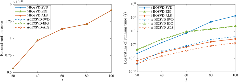
Figure 1: Reconstruction errors and running time of various low multilinear rank approximation algorithms for reconstructing random noisy low CP-rank tensors with gradually increased size.

In the experiments, we set the tensor size to be $J=I$ and $K=100I$ and gradually increase $I$ from $20$ to $100$ with step $20$. The truncation is set to $(R,R,R)$, where $R=0.2I$. We carry out the tests for 20 times and draw the averaged reconstruction errors and running time in Fig. 1. From the figure, it is observed that there is almost no difference in reconstruction error among all tested algorithms, indicating that the proposed ALS-based methods can maintain the accuracy of the original ones. In terms of the running time, $t$-HOSVD-ALS is $3.4\times\sim 50.9\times$ faster than $t$-HOSVD-SVD, and $6.9\times\sim 13.6\times$ faster than $t$-HOSVD-EIG, respectively. For $st$-HOSVD, the speedup of $st$-HOSVD-ALS is $1.0\times\sim 3.0\times$ and $9.8\times\sim 22.3\times$, as compared to $st$-HOSVD-SVD and $st$-HOSVD-EIG, respectively. We remark that the original algorithms behaves very differently in $t$-HOSVD and $st$-HOSVD. In particular, changing from $t$-HOSVD-EIG to $st$-HOSVD-EIG leads to little performance improvement. This is because the efficiency of eigen-decomposition of the Gram matrix is strongly dependent on the size of the third mode of the input tensor, and the sequentially updated algorithm is not able to help in this case.

5.1.2 Tucker model

Then we consider the base tesnor $\bm{\mathcal{A}}\in\mathbb{R}^{I_{1}\times I_{2}\times I_{3}\times I_{4}}$ constructed through the Tucker model in the following way:

$$\bm{\mathcal{A}}=\bm{\mathcal{G}}\times_{1}\bm{U}^{(1)}\times_{2}\bm{U}^{(2)}\times_{3}\bm{U}^{(3)}\times_{4}\bm{U}^{(4)},$$

where $\bm{\mathcal{G}}\in\mathbb{R}^{R_{1}\times R_{2}\times R_{3}\times R_{4}}$ is randomly generated core tensor whose elements follow the uniform distribution on interval $[5,10]$, and $\bm{U^{(i)}}\in\mathbb{R}^{I_{i}\times R_{i}},\ i=1,2,3,4$ are column orthogonal factor matrices.

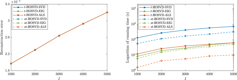
Figure 2: Reconstruction errors and running time of various low multilinear rank approximation algorithms for reconstructing random noisy low multilinear-rank tensors with gradually increased size.

In the experiments, we set $I_{2}=I_{3}=I_{4}=100$ and gradually increase $I_{1}=I$ from $1,000$ to $5,000$ with step $1,000$. The truncation is set to be $(R,10,10,10)$, where $R=0.01I$. We again carry out the tests for 20 times, and draw the averaged reconstruction errors and running time in Fig.2. From the figure, we observe that the reconstruction errors of all tested algorithms are nearly identical. For $t$-HOSVD, the performance of $t$-HOSVD-ALS is close to that of $t$-HOSVD-EIG, and they are both $10.3\times$ faster than $t$-HOSVD-SVD. For $st$-HOSVD, the speedup of $st$-HOSVD-ALS is $26.5\times$ and $3.5\times$, as compared to $st$-HOSVD-SVD and $st$-HOSVD-EIG, respectively.

5.2 Classification of handwritten digits

The second set of experiments is designed for testing the capability of the original $t$- and $st$-HOSVD algorithms and the proposed ALS-based ones on handwritten digits classification. It was studied that low multilinear rank approximation can be applied to compress the training data of images so that the core tensor can be utilized for image classification on the test data Savas2007 . In the tests, we use the MNIST database MNIST ; LeCun1998 of handwritten digits. We transfer the training dataset into a fourth-order tensor $\bm{\mathcal{A}}\in\mathbb{R}^{28\times 28\times 5000\times 10}$, where the first- and second-mode are the texel modes, the third-mode corresponds to training images, and the fourth-mode represents image categories. In the tests, the truncation is fixed to be $(8,8,142,10)$, which is close to the setting of the reference work Savas2007 . We measure the classification accuracy of a classification algorithm as the percentage of the test images that is correctly classified.

Table 2: Approximation error, classification accuracy and training time of various low multilinear rank approximation algorithms for handwritten digits classification of the MNIST database.

Algorithms	$t$-HOSVD			$st$-HOSVD
	SVD	EIG	ALS	SVD	EIG	ALS
Approximation error	$0.4330$	$0.4330$	$0.4335$	$0.4288$	$0.4288$	$0.4291$
Classification accuracy ($\%$)	$95.45$	$95.45$	$95.45$	$95.36$	$95.36$	$95.35$
Training time (s)	$18.97$	$5.38$	$3.30$	$4.07$	$5.12$	$1.53$

We run the test for $20$ times and record the averaged approximation error, classification accuracy and running time of the tested algorithms in Table 2. From the table it can be seen that the approximation errors and classification accuracies of all tested algorithms are almost indistinguishable, which again validates the accuracy of the proposed methods. Table 2 also shows that the ALS-based methods are fastest in terms of training time. Specifically, the ALS-based approaches are on average $1.6\times\sim 5.7\times$ and $2.7\times\sim 3.3\times$ faster than the original $t$-HOSVD and $st$-HOSVD algorithms, respectively.

5.3 Compression of tensors arising from fluid dynamics simulations

The purpose of this set of experiments is to examine the performance of different low multilinear rank approximation algorithms for compressing tensors generated from the simulation results of a lid-driven cavity flow, which is a standard benchmark for incompressible fluid dynamics Burggraf1966 . The simulation is done in a square domain of length $1$ m with the speed of the top plate setting to $1$ m/s and all other boundaries no flip. The kinematic viscosity is $\nu=1.0\times 10^{-4}$ m²/s, and the fluid properties is assumed to be laminar. We use the OpenFOAM software package Weller to conduct the simulation on a uniform grid with $100$ grid cells in each direction. The simulation is run with time step $\Delta t=1.0\times 10^{-4}$ s and terminated at $t=1.0$ s. We record the magnitude of velocity at every time step. The simulation results of the lid-driven cavity flow are stored in a third-order tensor of size $100\times 100\times 10000$. To test the tensor approximation algorithms, we fix the truncation to $(20,20,20)$, corresponding to a compression ratio of $12,500:1$.

First, we examine whether $(R_{1},R_{2},R_{3})=(20,20,20)$ is a suitable truncation for the input tensor. Since the dimensions of the first two modes are both $100$, we consider $R_{1}=R_{2}=20$ is a relatively proper choice. And $R_{3}=20$ is remained to test for the third dimension of length $10,000$. Therefore, we perform a test to see how the approximation error varies as $R_{3}$ changes gradually from $10$ to $100$. The test results are shown in Fig. 3 , from which it can be observed that $R_{3}=20$ is also proper for the third dimension.

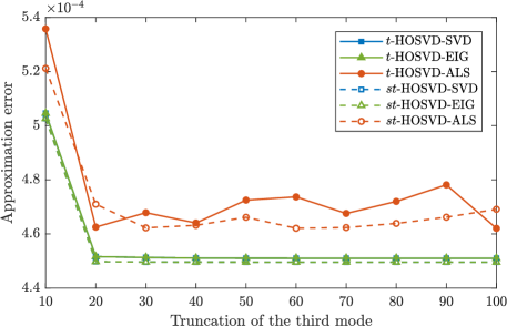
Figure 3: Approximation errors of $t$-HOSVD and $st$-HOSVD with gradually increased $R_{3}$.

Table 3: Relative residuals and running time of various low multilinear rank approximation algorithms for compressing tensors arising from fluid dynamics simulations with different tolerance parameters.

$t$-HOSVD	SVD	EIG	ALS
			$\eta=10^{-2}$	$\eta=10^{-4}$	$\eta=10^{-6}$
Relative residual ($\times 10^{-4}$)	$4.5161$	$4.5161$	$15.7422$	$4.6240$	$4.5225$
Running time (s)	$118.35$	$23.61$	$1.41+0.96$	$2.21+0.96$	$3.964+0.96$
$st$-HOSVD	SVD	EIG	ALS
			$\eta=10^{-2}$	$\eta=10^{-4}$	$\eta=10^{-6}$
Relative residual ($\times 10^{-4}$)	$4.4976$	$4.4976$	$14.2730$	$4.7139$	$4.5044$
Running time (s)	$3.44$	$21.70$	$0.73$	$1.16$	$1.82$

Next, we study the efficiency of tested algorithms under different accuracy requirements. We run the test for 20 times with tolerance parameter $\eta$ adjusted to different values and record the averaged relative residual and running time for each value of $\eta$; the test results are listed in Table 3. Also provided in the table is the extra cost of computing the singular vectors for $t$-HOSVD-ALS, if requested. From the table we have the following observations.

• The relative residuals and running time of the original $t$- and $st$-HOSVD algorithms are independent of the change of the tolerance parameter $\eta$. This is due to the usage of Krylov subspace method for computing matrix truncated SVD or eigen-decomposition.

• For the ALS-based methods, the relative residuals and the running time both depend on $\eta$. With $\eta$ decreased, the relative residuals are reduced to a similar level that the original algorithms can attain but more running time is required.

• The ALS-based algorithms are the fastest in all tests. It can achieve $6.1\times\sim 45.6\times$ speedup for $t$-HOSVD and $2.3\times\sim 18.4\times$ speedup for $st$-HOSVD, respectively.

• The overhead of computing the singular vectors for $t$-HOSVD-ALS is independent of the ALS tolerance and is relatively low.

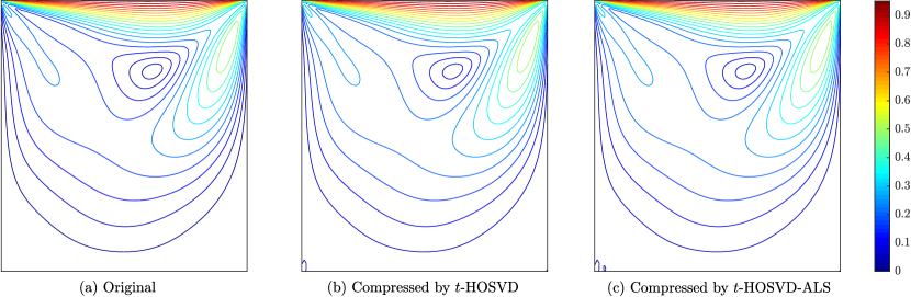
Figure 4: The original and compressed data at $t=0.5$ s for compressing tensors arising from fluid dynamics simulations with tolerance parameter $\eta=10^{-4}$.

It seems from the tests that despite the excellent performance of the proposed ALS-based methods, the strong dependency between the sustained performance and the tolerance parameter $\eta$ could eventually lead to poor performance if $\eta$ is very small. In practice the $t$- or $st$-HOSVD algorithm is often used as the initial guess of a supposedly more accurate iterative method such as HOOI. In this case it is not necessary to use a very tight tolerance parameter. To examine whether $\eta=10^{-4}$ is a suitable choice for the ALS-based algorithms in the same tests, we draw in Fig. 4 the contours of the original and compressed velocity data at $t=0.5$ s. It clearly shows that when $\eta=10^{-4}$, the compressed results are consistent with each other with very little discrepancy. In fact, the measured maximum differences between the original data and the compressed data obtained by $t$-HOSVD and that by $t$-HOSVD-ALS are around $1.58\times 10^{-3}$ and $1.33\times 10^{-3}$, respectively, which are very small considering that the compression ratio is over five orders of magnitude.

Table 4: A comparison of HOOI results for compressing tensors arising from fluid dynamics simulations with initial solutions provided by various low multilinear rank approximation algorithms.

Algorithm	Relative residual		Number of HOOI iterations
	Initial	Final
$t$-HOSVD-SVD	$4.5161\times 10^{-4}$	$4.4807\times 10^{-4}$	$9.0$
$t$-HOSVD-EIG	$4.5161\times 10^{-4}$	$4.4807\times 10^{-4}$	$7.0$
$t$-HOSVD-ALS	$4.6260\times 10^{-4}$	$4.4807\times 10^{-4}$	$6.0$
$st$-HOSVD-SVD	$4.4976\times 10^{-4}$	$4.4807\times 10^{-4}$	$5.0$
$st$-HOSVD-EIG	$4.4976\times 10^{-4}$	$4.4807\times 10^{-4}$	$6.0$
$st$-HOSVD-ALS	$4.5044\times 10^{-4}$	$4.4807\times 10^{-4}$	$7.0$

To further investigate the applicability of the compressed results, we use the computed low multilinear rank approximation with tolerance parameter $\eta=10^{-4}$ as the initial guess of the HOOI method with stopping criterion $10^{-12}$. The HOOI method is obtained from the tucker_als function of the Tensor Toolbox v3.1 Bader . The test results are presented in Table 4, in which we list the relative residuals with the $t$- and $st$-HOSVD provided initial guesses, the final relative residuals of HOOI, and the number of HOOI iterations, all averaged on 20 independent runs. From the table we can see that although the initial residual provided by the ALS-based algorithms are slightly larger than those provided by the original $t$- and $st$-HOSVD methods, same final residuals can be achieved after HOOI iterations nevertheless. And more importantly, the required numbers of HOOI iterations are insensitive to which specific $t$- and $st$-HOSVD algorithms, original or not, are used as shown in the tests. In other words, the proposed ALS-based methods are able to deliver similar results as the original ones when applying in HOOI, even when the tolerance parameter is relatively loose.

5.4 Parallel performance

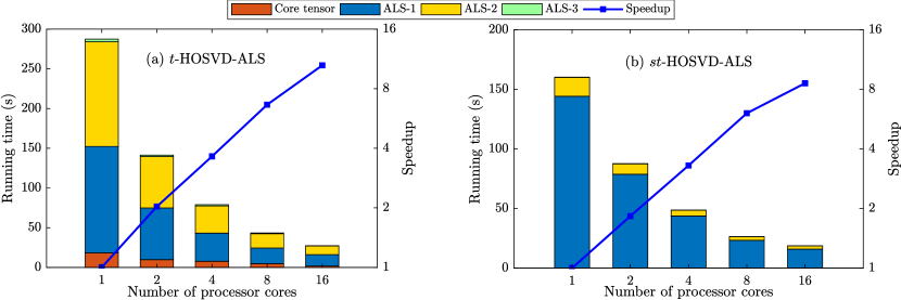
Figure 5: The running time and speedup of the ALS-based truncated HOSVD algorithms for compressing low multilinear rank tensor on a parallel computer.

An advantage of the proposed ALS-based methods is that they are easy to parallelize. To examine the parallel performance, in this experiment, we implement the $t$-HOSVD-ALS and $st$-HOSVD-ALS algorithms in C++ with OpenMP multi-threading parallelization OpenMP . The involved linear algebra operations are available with parallelization from the Intel MKL Intel ; Wang2014 and the open-source ARMADILLO Sanderson2016 ; Sanderson2018 libraries. In the test, the input tensor is generated by ttensor in the Tensor Toolbox, whose size is $5000\times 5000\times 50$ and the multilinear rank is $(500,500,5)$. We break down the running time into different portions, including the ALS iterations along the three dimensions (ALS-$i$, $i\in\{1,2,3\}$) and the calculation of the core tensor. The test results are drawn in Fig. 5. Also shown in the figures is the parallel scalability of the proposed algorithms.

From the figure, it can be seen that the proposed $t$-HOSVD-ALS and $st$-HOSVD-ALS can both scale well. In particular, $t$-HOSVD-ALS and $st$-HOSVD-ALS can achieve speedups of $10.50\times$ and $8.59\times$ as the number of processor cores is increased from 1 to 16, respectively. Moreover, in both algorithms the ALS iterations, as the major costs, are accelerated efficiently with the increased number of processor cores. Another observation is that there is a slight drop of parallel efficiency when using 16 processor cores, which is caused by the fact that the factor matrix $\bm{U}^{(n)}$ is usually tall and skinny due to the low multilinear rank structure of tensor. Overall, the test results demonstrate that the proposed ALS-based algorithms are parallelization friendly and have good potential to scale further on larger high-performance computers.

6 Conclusions

In this paper, we proposed a class of ALS-based algorithms for efficiently calculating the low multilinear rank approximation of tensors. Compared with the original $t$-HOSVD and $st$-HOSVD algorithms, the proposed algorithms are superior in several ways. First, by eliminating the redundant computations of the singular vectors, the overall costs of the algorithms are substantially reduced. Second, the proposed algorithms are more flexible with adjustable convergence tolerance, which is especially useful when the algorithms are used to generate initial solutions for iterative methods such as HOOI. Third, the proposed algorithms are free of the notorious date explosion issue due to the fact that the ALS procedure does not explicitly require the intermediate matrices. And fourth, the ALS-based approaches are parallelization friendly on high-performance computers. Theoretical analysis shows that the ALS iteration in the proposed algorithms is q-linear convergent with a relatively wide convergence region. Numerical experiments with both synthetic and real-world tensor data demonstrate that proposed ALS-based algorithms can substantially reduce the total cost of low multilinear rank approximation and are highly parallelizable.

Possible future works could include applying of the proposed ALS-based algorithms to more applications, among which we are especially interested in large-scale scientific computing. It would also be of interest to study randomization techniques to further improve the performance of the proposed algorithms, considering the fact that solving multiple least squares problems with different right-hand sides is the major cost. Some of the ideas presented in this work, such as the utilization of ALS for solving the intermediate low rank approximation problem, might be extended to other tensor decomposition models such as tensor-train (TT) and hierarchical Tucker (HT) decompositions.

Declarations

Funding This study was funded in part by Guangdong Key R&D Project (#2019B121204008), Beijing Natural Science Foundation (#JQ18001) and Beijing Academy of Artificial Intelligence.

Conflicts of Interest The authors declare that they have no conflict of interest.

Availability of Data and Material The datasets generated and analyzed during the current study are available from the corresponding author on reasonable request.

Code Availability The code used in the current study is available from the corresponding author on reasonable request.

Appendix A Proof of Theorem 1

Based on the assumption of Theorem 1, $\bm{L}_{k}$ is nonsingular and $\bm{L}_{k}^{T}\bm{L}_{k}$ is positive definite. Thus, the iterative form of Algorithm 3 is

$$\begin{split}\bm{R}_{k}=\bm{A}^{T}\bm{L}_{k}(\bm{L}_{k}^{T}\bm{L}_{k})^{-1},\\ \bm{L}_{k+1}=\bm{AR}_{k}(\bm{R}_{k}^{T}\bm{R}_{k})^{-1},\end{split}$$ (A.1)

i.e.,

$$\bm{L}_{k+1}=\bm{AA}^{T}\bm{L}_{k}(\bm{L}_{k}^{T}\bm{AA}^{T}\bm{L}_{k})^{-1}(\bm{L}_{k}^{T}\bm{L}_{k}).$$ (A.2)

Suppose that the full SVD of $\bm{A}$ is $\bm{A}=\bm{U}\bm{\Sigma}\bm{V}^{T}$, where

$$\bm{U}=[\bm{U}_{1},\bm{U}_{2}],\ \bm{V}=[\bm{V}_{1},\bm{V}_{2}],\,\bm{\Sigma}=\left(\begin{array}[]{cc}\bm{\Sigma}_{1}&0\\ 0&\bm{\Sigma}_{2}\\ \end{array}\right).$$

Then from (A.2), we have

$$\bm{U}^{T}\bm{L}_{k+1}=\bm{U}^{T}\bm{AVV}^{T}\bm{A}^{T}\bm{UU}^{T}\bm{L}_{k}(\bm{L}_{k}^{T}\bm{UU}^{T}\bm{AVV}^{T}\bm{A}^{T}\bm{UU}^{T}\bm{L}_{k})^{-1}(\bm{L}_{k}^{T}\bm{UU}^{T}\bm{L}_{k}),$$ (A.3)

which can be rewritten into block form

$$\left(\begin{array}[]{c}\bm{L}_{k+1}^{(1)}\\ \bm{L}_{k+1}^{(2)}\\ \end{array}\right)=\left(\begin{array}[]{cc}\bm{\Sigma}_{1}^{2}&0\\ 0&\bm{\Sigma}_{2}\bm{\Sigma}_{2}^{T}\\ \end{array}\right)\left(\begin{array}[]{c}\bm{L}_{k}^{(1)}\\ \bm{L}_{k}^{(2)}\\ \end{array}\right)(\bm{L}_{k}^{(1)T}\bm{\Sigma}_{1}^{2}\bm{L}_{k}^{(1)}+\bm{L}_{k}^{(2)T}\bm{\Sigma}_{2}\bm{\Sigma}_{2}^{T}\bm{L}_{k}^{(2)})^{-1}(\bm{L}_{k}^{(1)T}\bm{L}_{k}^{(1)}+\bm{L}_{k}^{(2)T}\bm{L}_{k}^{(2)}).$$

It then follows that

$$\begin{split}\bm{L}_{k+1}^{(1)}&=\bm{\Sigma}_{1}^{2}\bm{L}_{k}^{(1)}(\bm{L}_{k}^{(1)T}\bm{\Sigma}_{1}^{2}\bm{L}_{k}^{(1)}+\bm{L}_{k}^{(2)T}\bm{\Sigma}_{2}\bm{\Sigma}_{2}^{T}\bm{L}_{k}^{(2)})^{-1}(\bm{L}_{k}^{(1)T}\bm{L}_{k}^{(1)}+\bm{L}_{k}^{(2)T}\bm{L}_{k}^{(2)}),\\ \bm{L}_{k+1}^{(2)}&=\bm{\Sigma}_{2}\bm{\Sigma}_{2}^{T}\bm{L}_{k}^{(2)}(\bm{L}_{k}^{(1)T}\bm{\Sigma}_{1}^{2}\bm{L}_{k}^{(1)}+\bm{L}_{k}^{(2)T}\bm{\Sigma}_{2}\bm{\Sigma}_{2}^{T}\bm{L}_{k}^{(2)})^{-1}(\bm{L}_{k}^{(1)T}\bm{L}_{k}^{(1)}+\bm{L}_{k}^{(2)T}\bm{L}_{k}^{(2)}).\end{split}$$ (A.4)

Furthermore,

$$\begin{split}&(\bm{L}_{k}^{(1)T}\bm{\Sigma}_{1}^{2}\bm{L}_{k}^{(1)}+\bm{L}_{k}^{(2)T}\bm{\Sigma}_{2}\bm{\Sigma}_{2}^{T}\bm{L}_{k}^{(2)})^{-1}\\ =&(\bm{I}+(\bm{L}_{k}^{(1)T}\bm{\Sigma}_{1}^{2}\bm{L}_{k}^{(1)})^{-1}(\bm{L}_{k}^{(2)T}\bm{\Sigma}_{2}\bm{\Sigma}_{2}^{T}\bm{L}_{k}^{(2)}))^{-1}(\bm{L}_{k}^{(1)T}\bm{\Sigma}_{1}^{2}\bm{L}_{k}^{(1)})^{-1}\\ =&(\bm{I}+\sum\limits_{n=1}^{\infty}(-1)^{n}((\bm{L}_{k}^{(1)T}\bm{\Sigma}_{1}^{2}\bm{L}_{k}^{(1)})^{-1}(\bm{L}_{k}^{(2)T}\bm{\Sigma}_{2}\bm{\Sigma}_{2}^{T}\bm{L}_{k}^{(2)}))^{n})(\bm{L}_{k}^{(1)T}\bm{\Sigma}_{1}^{2}\bm{L}_{k}^{(1)})^{-1}.\end{split}$$ (A.5)

Here we suppose that the distance between $\mathcal{R}(\bm{L}_{k})$ and $\mathcal{R}(\bm{U}_{2})$ is small enough, therefore can be denoted as $\delta_{k}$, which only depends on $\|\bm{L}_{k}^{(2)}\|_{2}$ (i.e., there exist two constants $\alpha,\ \beta>0$ such that $\alpha\delta_{k}\leq\|\bm{L}_{k}^{(2)}\|_{2}\leq\beta\delta_{k}$). We can then obtain the lower bound of the distance between $\mathcal{R}(\bm{L}_{k})$ and $\mathcal{R}(\bm{U}_{1})$, which is $\sqrt{1-\delta_{k}^{2}}$, and

$$\begin{split}\|\bm{L}_{k}^{(1)}\|_{2}\leq C_{1},\quad\|(\bm{L}_{k}^{(1)})^{-1}\|_{2}\leq\frac{C_{2}}{\sqrt{1-\delta_{k}^{2}}},\end{split}$$ (A.6)

where $C_{1},\ C_{2}$ are constants independent on $k$ and $\delta_{k}$. From (A.5) and (A.6), there exists a constant $C$ that is only dependent on $C_{1},\ C_{2}$ so that the following inequality holds.

$$(\bm{L}_{k}^{(1)T}\bm{\Sigma}_{1}^{2}\bm{L}_{k}^{(1)}+\bm{L}_{k}^{(2)T}\bm{\Sigma}_{2}\bm{\Sigma}_{2}^{T}\bm{L}_{k}^{(2)})^{-1}\leq(\bm{L}_{k}^{(1)T}\bm{\Sigma}_{1}^{2}\bm{L}_{k}^{(1)})^{-1}+\frac{C\delta_{k}^{2}}{(1-2\delta_{k}^{2})^{2}},$$ (A.7)

Further, from (A.7) and (A.4), assume that $\sigma_{r}>\sigma_{r+1}$, we have

$$\begin{split}\bm{L}_{k+1}^{(2)}\leq\frac{\bm{\Sigma}_{2}\bm{\Sigma}_{2}^{T}}{\sigma_{r}^{2}}\bm{L}_{k}^{(2)}(\bm{L}_{k}^{(1)T}\frac{\bm{\Sigma}_{1}^{2}}{\sigma_{r}^{2}}\bm{L}_{k}^{(1)})^{-1}(\bm{L}_{k}^{(1)T}\bm{L}_{k}^{(1)})+\hat{C}\left(\frac{\delta_{k}^{2}}{(1-2\delta_{k}^{2})^{2}}+\frac{\delta_{k}^{2}}{1-\delta_{k}^{2}}+\frac{\delta_{k}^{4}}{(1-2\delta_{k}^{2})^{2}}\right),\end{split}$$

where $\hat{C}$ is a constant. Clearly,

$$0<\bm{L}_{k}^{(1)T}\bm{L}_{k}^{(1)}\leq\bm{L}_{k}^{(1)T}\frac{\bm{\Sigma}_{1}^{2}}{\sigma_{r}^{2}}\bm{L}_{k}^{(1)},$$

and by Lemma 1, we have

$$\|(\bm{L}_{k}^{(1)T}\frac{\bm{\Sigma}_{1}^{2}}{\sigma_{r}^{2}}\bm{L}_{k}^{(1)})^{-1}(\bm{L}_{k}^{(1)T}\bm{L}_{k}^{(1)})\|_{2}\leq 1.$$

Since $\delta_{k}$ is small enough, we obtain

$$\begin{split}\|\bm{L}_{k+1}^{(2)}\|_{2}\leq\frac{\sigma_{r+1}^{2}}{\sigma_{r}^{2}}\|\bm{L}_{k}^{(2)}\|_{2}+\tilde{C}\delta_{k}^{2}\leq\frac{\sigma_{r+1}^{2}}{\sigma_{r}^{2}}\|\bm{L}_{k}^{(2)}\|_{2}+\frac{\tilde{C}}{\alpha^{2}}\|\bm{L}_{k}^{(2)}\|_{2}^{2},\end{split}$$ (A.8)

where $\alpha,\ \tilde{C}$ do not depend on $k$ and $\|\bm{L}_{k}^{(2)}\|_{2}$.

Denote

$$q=\frac{\sigma_{r+1}^{2}}{\sigma_{r}^{2}}+\frac{\tilde{C}}{\alpha^{2}}\|\bm{L}_{0}^{(2)}\|_{2}.$$

Since we assume that $\mathcal{R}(\bm{L}_{0})$ is close to $\mathcal{R}(\bm{U}_{1})$ enough, $\|\bm{U}_{2}^{T}\bm{L}_{0}\|_{2}$ is sufficiently small, i.e., $\|\bm{L}_{0}^{(2)}\|_{2}=o(1)$. In other words, we assume that $q<1$. From (A.8), we have

$$\|\bm{L}_{k+1}^{(2)}\|_{2}\leq q\|\bm{L}_{k}^{(2)}\|_{2}$$

for all $k$, which leads to

$$\lim\limits_{k\rightarrow+\infty}\|\bm{L}_{k}^{(2)}\|_{2}\rightarrow 0.$$

Combining with the assumption of $\bm{L}_{k}$, it is verified that $\mathcal{R}(\bm{L}_{k})$ is orthogonal to $\mathcal{R}(\bm{U}_{2})$ with $k\rightarrow+\infty$. Since the orthogonal complement space of $\mathcal{R}(\bm{U}_{2})$ is unique, we have

$$\mathcal{R}(\bm{L}_{k})=\mathcal{R}(\bm{U}_{1}),\ \ k\rightarrow+\infty,$$

where $\mathcal{R}(\bm{U}_{1})$ is the dominant subspace of $\bm{A}$. In other words, we have

$$\begin{split}\lim\limits_{k\rightarrow+\infty}\|\bm{L}_{k}\bm{L}_{k}^{{\dagger}}-\bm{U}_{1}\bm{U}_{1}^{T}\|_{2}=0,\end{split}$$

where $\bm{L}_{k}^{{\dagger}}$ is the pseudo-inverse of $\bm{L}_{k}$. Further, from the iterative form of the ALS method, we have

$$\bm{R}_{k}=\bm{A}^{T}(\bm{L}_{k}^{{\dagger}})^{T},$$

thus

$$\bm{L}_{k}\bm{R}_{k}^{T}=\bm{L}_{k}\bm{L}_{k}^{{\dagger}}\bm{A}\rightarrow\bm{U}_{1}\bm{U}_{1}^{T}\bm{A},\ k\rightarrow+\infty.$$

And since the Frobenius norm $\|\cdot\|_{F}$ is continuous,

$$\lim\limits_{k\rightarrow+\infty}\|\bm{A}-\bm{L}_{k}\bm{R}_{k}^{T}\|_{F}=\|\bm{A}-\bm{U}_{1}\bm{U}_{1}^{T}\bm{A}\|_{F}.$$

Since $\bm{U}_{1}\bm{U}_{1}^{T}\bm{A}$ is the exact solution of low rank approximation of $\bm{A}$, the convergence of the ALS method is proved.

From (A.8), we further confirm the $q$-linear convergence of the ALS method, with approximate convergence ratio $\sigma_{r+1}^{2}/\sigma_{r}^{2}$. ∎

Appendix B Proof of Theorem 2

The assumption of Theorem 1 implies that $\bm{L}_{k}$ is nonsingular at every iteration $k$. We assume that

$$\bm{L}_{k}^{(1)T}\bm{\Sigma}_{1}^{2}\bm{L}_{k}^{(1)}+\bm{L}_{k}^{(2)T}\bm{\Sigma}_{2}\bm{\Sigma}_{2}^{T}\bm{L}_{k}^{(2)}$$

is positive definite. Let $\varepsilon$ be a positive number such that $\sigma_{r}>\sigma_{r+1}-\varepsilon$. By (A.4), we know

$$\begin{split}\bm{L}_{k+1}^{(1)}&=\bm{\Sigma}_{1}^{2}\bm{L}_{k}^{(1)}(\bm{L}_{k}^{(1)T}\bm{\Sigma}_{1}^{2}\bm{L}_{k}^{(1)}+\bm{L}_{k}^{(2)T}\bm{\Sigma}_{2}\bm{\Sigma}_{2}^{T}\bm{L}_{k}^{(2)})^{-1}(\bm{L}_{k}^{(1)T}\bm{L}_{k}^{(1)}+\bm{L}_{k}^{(2)T}\bm{L}_{k}^{(2)}),\\ \bm{L}_{k+1}^{(2)}&=\bm{\Sigma}_{2}\bm{\Sigma}_{2}^{T}\bm{L}_{k}^{(2)}(\bm{L}_{k}^{(1)T}\bm{\Sigma}_{1}^{2}\bm{L}_{k}^{(1)}+\bm{L}_{k}^{(2)T}\bm{\Sigma}_{2}\bm{\Sigma}_{2}^{T}\bm{L}_{k}^{(2)})^{-1}(\bm{L}_{k}^{(1)T}\bm{L}_{k}^{(1)}+\bm{L}_{k}^{(2)T}\bm{L}_{k}^{(2)}),\end{split}$$ (B.1)

which means

$$\begin{split}\bm{L}_{k+1}^{(1)}=\frac{\bm{\Sigma}_{1}^{2}}{(\sigma_{r}-\varepsilon)^{2}}\bm{L}_{k}^{(1)}(\bm{L}_{k}^{(1)T}\frac{\bm{\Sigma}_{1}^{2}}{(\sigma_{r}-\varepsilon)^{2}}\bm{L}_{k}^{(1)}+\bm{L}_{k}^{(2)T}\frac{\bm{\Sigma}_{2}\bm{\Sigma}_{2}^{T}}{(\sigma_{r}-\varepsilon)^{2}}\bm{L}_{k}^{(2)})^{-1}(\bm{L}_{k}^{(1)T}\bm{L}_{k}^{(1)}+\bm{L}_{k}^{(2)T}\bm{L}_{k}^{(2)}),\\ \bm{L}_{k+1}^{(2)}=\frac{\bm{\Sigma}_{2}\bm{\Sigma}_{2}^{T}}{(\sigma_{r}-\varepsilon)^{2}}\bm{L}_{k}^{(2)}(\bm{L}_{k}^{(1)T}\frac{\bm{\Sigma}_{1}^{2}}{(\sigma_{r}-\varepsilon)^{2}}\bm{L}_{k}^{(1)}+\bm{L}_{k}^{(2)T}\frac{\bm{\Sigma}_{2}\bm{\Sigma}_{2}^{T}}{(\sigma_{r}-\varepsilon)^{2}}\bm{L}_{k}^{(2)})^{-1}(\bm{L}_{k}^{(1)T}\bm{L}_{k}^{(1)}+\bm{L}_{k}^{(2)T}\bm{L}_{k}^{(2)}).\end{split}$$

Clearly it holds that

$$\begin{split}\|\bm{L}_{k+1}^{(2)}\|_{2}\leq\frac{\sigma_{r+1}^{2}}{(\sigma_{r}-\varepsilon)^{2}}\|\bm{L}_{k}^{(2)}\|_{2}\end{split}$$ (B.2)

under the condition that

$$\bm{L}_{k}^{(1)T}\bm{L}_{k}^{(1)}+\bm{L}_{k}^{(2)T}\bm{L}_{k}^{(2)}\leq\bm{L}_{k}^{(1)T}\frac{\bm{\Sigma}_{1}^{2}}{(\sigma_{r}-\varepsilon)^{2}}\bm{L}_{k}^{(1)}+\bm{L}_{k}^{(2)T}\frac{\bm{\Sigma}_{2}\bm{\Sigma}_{2}^{T}}{(\sigma_{r}-\varepsilon)^{2}}\bm{L}_{k}^{(2)}.$$ (B.3)

If $\bm{L}_{k}^{(1)}$ is nonsingular, then (B.3) implies

$$(\bm{L}_{k}^{(2)}(\bm{L}_{k}^{(1)})^{-1})^{T}(\bm{I}-\frac{\bm{\Sigma}_{2}\bm{\Sigma}_{2}^{T}}{(\sigma_{r}-\varepsilon)^{2}})(\bm{L}_{k}^{(2)}\bm{L}_{k}^{(1)-1})\leq\frac{\bm{\Sigma}_{1}^{2}}{(\sigma_{r}-\varepsilon)^{2}}-\bm{I}.$$ (B.4)

It follows to see that

$$\|\bm{L}_{k}^{(2)}(\bm{L}_{k}^{(1)})^{-1}\|_{2}\leq\sqrt{\frac{\sigma_{r}^{2}-(\sigma_{r}-\varepsilon)^{2}}{(\sigma_{r}-\varepsilon)^{2}-\sigma_{min}^{2}}}$$ (B.5)

is a sufficient condition of (B.4).

Next we will prove that if the initial guess $\bm{L}_{0}$ satisfies condition (B.5), then $\bm{L}_{k}^{(1)}$ is nonsingular and (B.2) is satisfied at every iteration $k$.

Provided that $\bm{L}_{0}$ satisfies (B.5), we obtain

$$\|\bm{L}_{1}^{(2)}\|_{2}\leq\frac{\sigma_{r+1}^{2}}{(\sigma_{r}-\varepsilon)^{2}}\|\bm{L}_{0}^{(2)}\|_{2}.$$ (B.6)

And according to the proof of Theorem 1, we know $\bm{L}_{1}^{(1)}$ is also nonsigular, which implies

$$\bm{L}_{1}^{(1)T}\bm{\Sigma}_{1}^{2}\bm{L}_{1}^{(1)}+\bm{L}_{1}^{(2)T}\bm{\Sigma}_{2}\bm{\Sigma}_{2}^{T}\bm{L}_{1}^{(2)}$$

is positive definite. Then by (B.1), we have

$$\|\bm{L}_{1}^{(2)}(\bm{L}_{1}^{(1)})^{-1}\|_{2}\leq\|\bm{\Sigma}_{2}\bm{\Sigma}_{2}^{T}\bm{L}_{0}^{(2)}(\bm{L}_{0}^{(1)})^{-1}\bm{\Sigma}_{1}^{-2}\|_{2}\leq\frac{\sigma_{r+1}^{2}}{\sigma_{r}^{2}}\|\bm{L}_{0}^{(2)}(\bm{L}_{0}^{(1)})^{-1}\|_{2}\leq\sqrt{\frac{\sigma_{r}^{2}-(\sigma_{r}-\varepsilon)^{2}}{(\sigma_{r}-\varepsilon)^{2}-\sigma_{min}^{2}}}.$$ (B.7)

Analogously, we can prove that for every iteration $k$, $\bm{L}_{k}^{(1)}$ is nonsingular, i.e., $\bm{L}_{k}^{(1)T}\bm{\Sigma}_{1}^{2}\bm{L}_{k}^{(1)}+\bm{L}_{k}^{(2)T}\bm{\Sigma}_{2}\bm{\Sigma}_{2}^{T}\bm{L}_{k}^{(2)}$ is positive definite, and (B.5) is satisfied. Since (B.5) is a sufficient condition of (B.4) and (B.3), inequality (B.2) is true at every iteration $k$, which implies that

$$\lim\limits_{k\rightarrow 0}\|\bm{L}_{k}\bm{L}_{k}^{\dagger}-\bm{U}_{1}\bm{U}_{1}^{T}\|_{2}=0.$$

The rest part of the proof is analogous to the proof of Theorem 1, which is omitted for brevity. ∎

Appendix C Proof of Theorem 3

In Algorithm 4, $\bm{U}^{(n)}$ is obtained from the rank-$R_{n}$ approximation of $\bm{A}_{(n)}$, which is done in an iterative manner and allows a tolerance parameter $\eta_{n}$. Therefore, we have

$$\|\bm{A}_{(n)}-\bm{L}^{*}\bm{R}^{*T}\|_{F}^{2}\leq\eta_{n}^{2}\|\bm{\mathcal{A}}\|_{F}^{2}+\gamma_{n},$$ (C.1)

where $\bm{L}^{*}$ and $\bm{R}^{*}$ are the same as in Algorithm 4. Note that $\bm{R}$ is updated by solving a multi-side least squares problem

$$\min\limits_{\bm{R}}\|\bm{A}_{(n)}-\bm{LR}^{T}\|_{F},$$

whose exact solution is $\bm{R}=\bm{A}_{(n)}^{T}(\bm{L}^{\dagger})^{T}$. Thus

$$\|\bm{A}_{(n)}-\bm{L}^{*}\bm{R}^{*T}\|_{F}=\|\bm{A}_{(n)}-\bm{L}^{*}\bm{L}^{*\dagger}\bm{A}_{(n)}\|_{F},$$ (C.2)

where $\bm{L}^{*}\bm{L}^{*\dagger}$ represents an orthogonal projection on subspace $\mathcal{R}(\bm{L}^{*})$. Consequently, by (C.1), (C.2) and (4.3), we have

$$\|\hat{\bm{\mathcal{A}}}-\bm{\mathcal{A}}\|_{F}^{2}\leq\sum\limits_{n=1}^{N}(\eta_{n}^{2}\|\bm{A}_{(n)}\|_{F}^{2}+\gamma_{n}),$$

which means

$$\frac{\|\hat{\bm{\mathcal{A}}}-\bm{\mathcal{A}}\|_{F}^{2}}{\|\bm{\mathcal{A}}\|_{F}^{2}}\leq\sum\limits_{n=1}^{N}(\eta_{n}^{2}+\frac{\gamma_{n}}{\|\bm{\mathcal{A}}\|_{F}^{2}}).$$

Combining with (4.3), we obtain (4.4).

The error analysis of Algorithm 5 can be analogously done. ∎

References

- (1) Intel Math Kernel Library Reference Manual [EQ/OL]. URL http://developer.intel.com
- (2) OpenFoam 2018, Version 6. URL https://openfoam.org
- (3) OpenMP application program interface, Version 4.0, OpenMP Architecture Review Board (July, 2013). URL http://www.openmp.org
- (4) Austin, W., Ballard, G., Kolda, T.G.: Parallel tensor compression for large-scale scientific data. In: IEEE International Parallel and Distributed Processing Symposium, pp. 912–922. IEEE (2016)
- (5) Bader, B.W., Kolda, T.G., et.al.: MATLAB Tensor Toolbox Version 3.1. Available online (2019). URL https://www.tensortoolbox.org
- (6) Baglama, J., Reichel, L.: Augmented implicitly restarted Lanczos bidiagonalization methods. SIAM J. Sci. Comput. 27(1), 19–42 (2005)
- (7) Beckmann, C., Smith, S.: Tensorial extensions of independent component analysis for multisubject FMRI analysis. Neuroimage 25(1), 294–311 (2005)
- (8) Beylkin, G., Mohlenkamp, M.J.: Numerical operator caculus in higher dimensions. Proc. Natl. Acad. Sci. 99, 10246–10251 (2002)
- (9) Bro, R.: Review on multiway analysis in chemistry—2000–2005. Crit. Rev. Anal. Chem. 36, 279–293 (2006)
- (10) B.Savas, Eldén, L.: Handwritten digit classification using higher order singular value decomposition. Pattern Recognition 40, 993–1003 (2007)
- (11) Burggraf, R.: Analytical and numerical studies of the structure of steady separated flows. J. Fluid Mechanics 24(1), 113–151 (1966)
- (12) Carroll, J.D., Chang, J.J.: Analysis of individual differences in multidimensional scaling via an -way generalization of “Eckart-Young” decomposition. Psychometrika 35, 283–319 (1970)
- (13) Charalampous, K., Gasteratos, A.: A tensor-based deep learning framework. Image and Vision Computing 32(11), 916–929 (2014)
- (14) Cullum, J., Willoughby, R., Lake, M.: A Lanczos algorithm for computing singular values and vectors of large matrices. SIAM J. Sci. Stat. Comput. 4(2), 197–215 (1983)
- (15) De Lathauwer, L., De Moor, B., Vandewalle, J.: A multilinear singular value decomposition. SIAM J. Matrix Anal. Appl. 21(4), 1253–1278 (2000)
- (16) De Lathauwer, L., De Moor, B., Vandewalle, J.: On the best rank-1 and rank- approximation of higher-order tensors. SIAM J. Matrix Anal. Appl. 21, 1324–1342 (2000)
- (17) De Lathauwer, L., Vandewalle, J.: Dimensionality reduction in higher-order signal processing and rank- reduction in multilinear algebra. Linear Algebra Appl. 391, 31–55 (2004)
- (18) De Leeuw, J., Young, F., Takane, Y.: Additive structure in qualitative data: An alternating least squares method with optimal scaling features. Psychometrika 41, 471–503 (1976)
- (19) De Silva, V., Lim, L.H.: Tensor rank and the ill-posedness of the best low-rank approximation problem. SIAM J. Matrix Anal. Appl. 30(3), 1084–1127 (2008)
- (20) Ding, W., Wei, Y.: Solving multi-linear systems with -tensors. J. Sci. Comput. 68, 689–715 (2016)
- (21) Elden, L., Savas, B.: A Newton-Grassmann method for computing the best multilinear rank- approximation of a tensor. SIAM J. Matrix Anal. Appl. 31(2), 248–271 (2009)
- (22) Golub, G.H., Van Loan, C.F.: Matrix Computations Ed. 4th. Johns Hopkins University Press, Baltimore (2008)
- (23) Grasedyck, L.: Hierarchical singular value decomposition of tensors. SIAM J. Matrix Anal. Appl. 31(4), 2029–2054 (2010)
- (24) Hackbusch, W.: Numerical tensor calculus. Acta Numerica 23, 651–742 (2014)
- (25) Hackbusch, W., Khn, S.: A new scheme for the tensor representation. J. Fourier Anal. Appl. 15, 706–722 (2009)
- (26) Halko, N., Martinsson, P.G., Tropp, J.A.: Finding structure with randomness: Probabilistic algorithms for constructing approximate matrix decompositions. SIAM Rev. 53(2), 217–288 (2011)
- (27) Henrion, R.: Body diagonalization of core matrices in three-way principal components analysis: Theoretical bounds and simulation. J. Chemometrics 7, 477–494 (1993)
- (28) Hitchcock, F.L.: Multiple invariants and generalized rank of a -way matrix or tensor. J. Math. Phys. 7(1-4), 39–79 (1928)
- (29) Holtz, S., Rohwedder, T., Schneider, R.: The alternating linear scheme for tensor optimization in the tensor train format. SIAM J. Sci. Compt. 34(2), A683–A713 (2012)
- (30) Ishteva, M., Absil, P.A., Van Huffel, S., De Lathauwer, L.: Best low multlinear rank approximation of higher-order tensors, based on the Riemannian trust-region scheme. SIAM J. Matrix Anal. Appl. 31(1), 115–135 (2011)
- (31) Ishteva, M., De Lathauwer, L., Absil, P.A., Huffel, S.: Dimensionality reduction for higher-order tensors: Algorithms and applications. Int. J. Pure Appl. Math. 42(3), 337–343 (2012)
- (32) Ishteva, M., De Lathauwer, L., Absil, P.A., Huffel, S.V.: Differential-geometric Newton method for the best rank- approximation of tensors. Numer. Algor. 51, 179–194 (2009)
- (33) Jiang, J., Wu, H., Li, Y., Yu, R.: Three-way data resolution by alternating slice-wise diagonalization (ASD) method. J. Chemometrics 14, 15–36 (2000)
- (34) Khoromskij, B.N.: Tensors-structured numerical methods in scientific computing: Survey on recent advances. Chemometrics and Intelligent Laboratory Systems 110(1), 1–19 (2012)
- (35) Kiers, H.A.L.: Towards a standardized notation and terminology in multiway analysis. J. Chemometrics 14, 105–122 (2000)
- (36) Kolda, T.G., Bader, B.W.: Tensor decompositions and applications. SIAM Rev. 51(3), 455–500 (2009)
- (37) Kroonenberg, P.M.: Applied Multiway Data Analysis. John Wiley & Sons. Inc., New Jersey (2008)
- (38) Kroonenberg, P.M., De Leeuw., J.: Principal component analysis of three-mode data by means of alternating least squares algorithms. Psychometrika 45, 69–97 (1980)
- (39) LeCun, Y., C.Cortes, C.Burges: THE MNIST DATABASE of handwritten digits. URL http://yann.lecun.com/exdb/mnist/
- (40) LeCun, Y., L.Bottou, Y.Bengio, P.Haffner: Gradient-based learning applied to document recognition. Proceedings of the IEEE 84(11), 2278–2324 (1998)
- (41) Levin, J.: Three-mode factor analysis. Ph.D. thesis, University of Illinois, Urbana-Champaign (1963)
- (42) Li, J., Battaglino, C., Perros, I., Sun, J., Vuduc, R.: An input-adaptive and in-place approach to dense tensor-times-matrix multiply. In: Proceedings of the International Conference for High Performance Computing, 76, pp. 1–12. ACM (2015)
- (43) Mahoney, M.W.: Randomized algorithms for matrices and data. Foundations and Trends in MachineLearning 3(2), 123–224 (2011)
- (44) Mahoney, M.W., Drineas, P.: RandNLA: Randomized numerical linear algebra. Communications of the ACM 59(6), 80–90 (2016)
- (45) Novikov, A., Podoprikhin, D., Osokin, A., Vetrov, D.: Tensorizing neural networks. In: Annual Conference on Neural Information Processing Systems, vol. 1, pp. 442–450. ACM (2015)
- (46) Oh, J., Shin, K., E.Papalexakis, E., Faloutsos, C., Yu, H.: S-HOT: Scalable high-Order Tucker decomposition. In: Proceedings of the Tenth ACM International Conference on Web Search and Data Mining, pp. 761–770. ACM (2017)
- (47) Oh, S., Park, N., Jang, J., Sael, L., Kang, U.: High-performance tucker factorization on heterogeneous platforms. IEEE Transactions on Parallel and Distributed Systems 30(10), 2237–2248 (2019)
- (48) Oseledets, I.V., Tyrtyshnikov, E.E.: Breaking the curse of dimensionality, or how to use SVD in many dimensions. SIAM J. Sci. Comput. 31(5), 3744–3759 (2009)
- (49) Oseledetsv, I.V.: Tensor-train decomposition. SIAM J. Sci. Comput. 33(5), 2295–2317 (2011)
- (50) Rajbhandari, S., Nikam, A., Lai, P.W., Stock, K., Krishnamoorthy, S., Sadayappan, P.: A communication-optimal framework for contracting distributed tensors. In: Proceedings of the International Conference for High Performance Computing, Networking, Storage and Analysis, pp. 375–386. IEEE (2014)
- (51) Sanderson, C., Curtin, R.: Armadillo: A template-based C++ library for linear algebra. J. Open Source Software 1(2), 26 (2016)
- (52) Sanderson, C., Curtin, R.: A user-friendly hybrid sparse matrix class in C++. In: International Conference on Mathematical Software, Lecture Notes in Computer Science (LNCS), vol. 10931, pp. 422–430. Springer (2018)
- (53) Savas, B., Lim, L.H.: Quasi-Newton methods on Grassmannians and multilinear approximations of tensors. SIAM J. Sci. Comput. 32(6), 3352–3393 (2009)
- (54) Schatz, M.: Distributed tensor computations: Formalizing distributions, redistributions, and algorithm derivations. Ph.D. thesis, University of Texas, Austin (2015)
- (55) Shashua, A., Levin, A.: Linear image coding for regression and classification using the tensor-rank principle. In: IEEE Conference on Computer Vision and Pattern Recognition, pp. 42–49. IEEE (2001)
- (56) Sidiropoulos, N.D., De Lathauwer, L., Xiao, F., Huang, K.J., Papalexakis, E.E., Faloutsos, C.: Tensor decomposition for signal processing and machine learning. IEEE Trans. on Sig. Proc. 65(13), 3551–3582 (2017)
- (57) Smith, S., Ravindran, N., Sidiropoulos, N., Kapypis, G.: Efficient and parallel sparse tensor matrix multiplication. In: IEEE International Parallel and Distributed Processing Symposium, pp. 61–70. IEEE (2015)
- (58) Sorensen, D.: Implicit application of polynomial filters in a -step Arnoldi method. SIAM J. Matrix Anal. Appl. 13(1), 357–385 (1992)
- (59) Stewart, G.: A Krylov-Schur algorithm for large eigenproblems. SIAM J. Matrix Anal. Appl. 23(3), 601–614 (2001)
- (60) Szlam, A., Tulloch, A., Tygert, M.: Accurate low-rank approximations via a few iterations of alternating least squares. SIAM J. Matrix Anal. Appl. 38(2), 425–433 (2017)
- (61) Tucker, L.R.: Some mathematical notes on three-mode factor analysis. Psychometrika 31, 279–311 (1966)
- (62) Vannieuwenhoven, N., Vandebril, R., Meerbergen, K.: On the truncated multilinear singular value decomposition. Technical Report TW589, Department of Computer Science, Katholieke Universiteit Leuven, Leuven, Belgium (2011)
- (63) Vannieuwenhoven, N., Vandebril, R., Meerbergen, K.: A new truncation strategy for the higher-order singular value decomposition. SIAM J. Sci. Comput. 34(2), A1027–A1052 (2012)
- (64) Vasilescu, M.A.O., Terzopoulos, D.: Multilinear image analysis for facial recognition. In: Object recognition supported by user interaction for service robots, vol. 2, pp. 511––514. IEEE (2002)
- (65) Vervliet, N., Debals, O., Sorber, L., M. Van Barel, L. De Lathauwer: Tensorlab 3.0. Available online (2016). URL https://www.tensorlab.net
- (66) Vlasi, D., Brand, M., Pfister, H., Popovic, J.: Face transfer with multilinear models. In: ACM SIGGRAPH 2005 Papers, vol. 24, pp. 426––433. ACM (2005)
- (67) Wang, E., Zhang, Q., Shen, B., Zhang, G., Lu, X., Wu, Q., Wang, Y.: “Intel Math Kernel Library,” in High-Performance Computing on the . Springer pp. 167–188 (2014)
- (68) Wang, S.G., Wu, M.X., Jia, Z.Z.: Matrix Inequality Ed. 2th. Science Press, Beijing (2006)
- (69) Watkins, D.: The QR algorithm revisited. SIAM Rev. 50(1), 133–145 (2008)
- (70) Xu, Y.: On the convergence of higher-order orthogonal iteration. Linear and Multilinear Algebra 66(11), 2247–2265 (2018)
- (71) Young, F.W., Takane, Y., De Leeuw, J.: The principal components of mixed measurement level multivariate data: An alternating least squares method with optimal scaling features. Psychometrika 43, 279–281 (1978)
- (72) Zhang, T., Golub, G.H.: Rank-one approximation to high order tensors. SIAM J. Matrix Anal. Appl. 23(2), 534–550 (2001)