Dynamic Ridesharing in Peak Travel Periods

Abstract

The abstract goes here.

Abstract

In this paper, we propose and study a variant of the dynamic ridesharing problem with a specific focus on peak hours: Given a set of drivers and a set of rider requests, we aim to match drivers to each rider request by achieving two objectives: maximizing the served rate and minimizing the total additional distance, subject to a series of spatio-temporal constraints. Our problem can be distinguished from existing ridesharing solutions in three aspects: (1) Previous work did not fully explore the impact of peak travel periods where the number of rider requests is much greater than the number of available drivers. (2) Existing ridesharing solutions usually rely on single objective optimization techniques, such as minimizing the total travel cost (either distance or time). (3) When evaluating the overall system performance, the runtime spent on updating drivers’ trip schedules as per newly coming rider requests should be incorporated, while it is unfortunately excluded by most existing solutions. In order to achieve our goal, we propose an underlying index structure on top of a partitioned road network, and compute the lower bounds of the shortest path distance between any two vertices. Using the proposed index together with a set of new pruning rules, we develop an efficient algorithm to dynamically include new riders directly into an existing trip schedule of a driver. In order to respond to new rider requests more effectively, we propose two algorithms that bilaterally match drivers with rider requests. Finally, we perform extensive experiments on a large-scale test collection to validate the effectiveness and efficiency of the proposed methods.

1 Introduction

Millions of drivers provide transportation services for over ten million passengers every day at Didi Chuxing [1], which is a Chinese counterpart of UberPOOL [2]. In peak travel periods, Didi needs to match more than a hundred thousand passengers to drivers every second [3], and rider demand often greatly exceeds rider capacity. Two approaches can be used to mitigate this problem. The first method attempts to predict areas with high travel demands using historical data and statistical predictions or a heat map, and taxis are strategically deployed in the corresponding areas in advance. An alternative approach is to serve multiple riders with fewer vehicles using a ridesharing service: riders with similar routes and time schedules can share the same vehicle [4, 5]. According to statistical data from the Bureau of Infrastructure, Transport and Regional Economics [6], there are less than 1.6 persons per vehicle per kilometer in Australia. If only 10% of vehicles had more than one passenger, then it would reduce annual fuel consumption by 5.4% [7]. Therefore, increasing vehicle occupancy rates would provide many benefits including the reduction of gas house emissions. Moreover, it has been reported that a crucial imbalance exists in supply and demand in peak hour scenarios, where the rider demand is double the rider availability based on historical data statistical analysis at Didi Chuxing [8]. Alleviating traffic congestion challenges during peak commuter times will ultimately require significant government commitment dedicated to increasing the region’s investment in core transportation infrastructure [9]. In this paper, we focus on the dynamic ridesharing problem, specifically during peak hour travel periods.

From an extensive literature study, we make the following observations to motivate this work – (1) Existing ridesharing studies [10, 11] do not fully explore the scenario where the number of riders is much greater than the number of available drivers, and so the scalability of current solutions in this setting remains unclear. (2) Prior studies [12, 13, 10, 14, 15, 16] primarily focus on single objective optimization solutions, such as minimizing the total travel distance from the perspective of drivers [13, 14], or maximizing the served rate of ridesharing system [16]. In contrast, we aim to optimize two objectives: maximize the served rate and minimize the total additional distance. (3) Previous studies [13, 17, 18, 11, 19] report the processing time mainly based on the rider request matching time, but not the trip schedule update time, which encompasses a driver’s current trip schedule and the underlying index structure updates. However, in a dynamic ridesharing scenario where vehicles are continuously moving, accounting for these additional costs produces a more realistic comparison of the algorithms being studied.

Our goal in this work is to determine a series of trip schedules with the minimum total additional distance capable of accommodating as many rider requests as possible, under a set of spatio-temporal constraints. In order to achieve this goal, we must account for three features: (1) each driver has an initial location and trip schedule, but rider requests are being continuously generated in a streaming manner; (2) before a driver receives a new incoming rider request, the arrival time and location of the rider are unknown; (3) the driver and the rider should be informed at short notice about whether a matching is possible or not. Specifically, the driver should be notified quickly if a new rider is added, and similarly the rider should be informed quickly if her travel request can be fulfilled based on the current preference settings, such as waiting time tolerance to be picked up.

The following challenges arise in addressing this problem:

(1) How can we find eligible driver-rider matching pairs to maximize the served rate and also minimize the additional distance? If more rider requests are satisfied, it implies that the driver has to travel further to pick up more rider(s). For instance, if a driver $d$ already has passengers on board but receives a new rider request $r_{1}$, the driver might detour to pick up $r_{1}$, resulting in an increase in the served rate and the distance traveled.

(2) How can we make a decision on the best service sequence for a trip schedule? Every rider has their own maximum allowable waiting time, and detour time tolerance. When a rider request is served, these constraints should not be violated. For example, a rider request $r_{1}$ is already in the trip schedule of a driver $d$, but a new rider request $r_{2}$ is received while the driver is serving $r_{1}$. The driver needs to determine if $r_{2}$ can be picked up first without violating $r_{1}$’s constraints.

(3) How can we efficiently support the ridesharing problem for streaming rider requests? The time used for determining the updated trip schedule as per new rider requests should not exceed the time window size.

In order to address the above challenges, we make the following contributions:

• We define a variant of the dynamic ridesharing problem, which aims to optimize two objectives subject to a series of spatio-temporal constraints presented in Section 3. In addition, our work mainly focuses on a common yet important scenario where the number of drivers is insufficient to serve all riders in peak travel periods.

• We develop an index structure on top of a partitioned road network and compute the lower bound of the shortest path distance between any two vertices in constant time in Section 4. We then propose a pruning-based rider request insertion algorithm based on several pruning rules to accelerate the matching process in Section 5.

• We further propose two algorithms to find matchable and eligible driver-rider pairs, which aim to maximize the served rate and minimize the total additional distance, in Section 6.1 and Section 6.2 respectively.

• We conduct extensive experiments on a real-world dataset in order to validate the efficiency and effectiveness of our methods under different parameter settings in Section 7.

In addition, we review the related work in Section 2 and conclude the work in Section 8.

2 Related Work

Ridesharing has been intensively studied in recent years, in both static and dynamic settings. A typical formulation for the static ridesharing problem consists of designing drivers’ routes and schedules for a set of rider requests with departure and arrival locations known beforehand [20, 21, 22, 23], while the dynamic ridesharing problem is based on the setting that new riders are continuously added in a stream-wise manner [24, 25, 26, 27].

Static Ridesharing Problem. Ta et al. [12] defined two kinds of ridesharing models to maximize the shared route ratio, under the assumption that at most one rider can be assigned to a driver in the vehicle. Cheng et al. [15] proposed a utility-aware ridesharing problem, which can be regarded as a variant of the dial-a-ride problem [28, 29]. The aim was to maximize the riders’ satisfaction, which is defined as a linear combination of vehicle-related utility, rider-related utility, and trajectory-related utility, such as rider sharing preferences. Bei and Zhang [30] investigated the assignment problem in ridesharing and designed an approximation algorithm with a worst-case performance guarantee when only two riders can share a vehicle. In contrast, we focus primarily on the dynamic ridesharing problem, and allow the maximum number of riders to be greater than two.

Dynamic Ridesharing Problem. Several existing techniques are well illustrated and outlined by two recent surveys [31, 32]. We describe the literature in chronological order. Agatz et al. [33] explored a ride-share optimization problem in which the ride-share provider aims to minimize the total system-wide vehicle-miles. Xing et al. [16] studied a multi-agent system with the objective of maximizing the number of served riders. Kleiner et al. [34] proposed an auction-based mechanism to facilitate both riders and drivers to bid according to their preferences. Ma et al. [13, 35] proposed a dynamic taxi ridesharing service to serve each request by dispatching a taxi with the minimum additional travel distance incurred. Huang et al. [14] designed a kinetic tree to enumerate all possible valid trip schedules for each driver. Duan et al. [36] studied the personalized ridesharing problem which maximizes a satisfaction value defined as a linear function of distance and time cost. Zheng et al. [10] considered the platform profit as the optimization objective to be maximized by dispatching the orders to vehicles. Tong et al. [18] devised route plans to maximize the unified cost which consists of the total travel distance and a penalty for unserved requests. Chen et al. [11] considered both the pick-up time and the price to return multiple options for each rider request in dynamic ridesharing. Xu et al. [37] proposed an efficient rider insertion algorithm that minimizes the maximum flow time of all requests or minimizes the total travel time of the driver.

Our work is different from existing ridesharing studies in two aspects: (1) Our focus is the peak hours scenario where there are too few drivers to satisfy all of the rider requests, which has not been explored in previous work. Later in the experimental study we extend the state-of-the-art [11] to the peak hour scenario and show that our approach outperforms it in both efficiency and effectiveness. (2) Most previous studies aim to optimize a single objective [14, 33, 13, 16, 10, 15, 37] or a customized linear function [36, 18]. This differs from our problem scenario where we solve the dual-objective optimization problem. Chen et al. [11] also considered two criteria (price and pick-up time) from the perspective of riders, but not the same criteria (served rate and additional distance) as we use to satisfy riders, drivers and ridesharing system requirements. In our problem, riders can provide their personal sharing preferences by giving constraint values, such as waiting time tolerance, drivers and ridesharing system expect to serve more riders with less detour distance, which coincides with our goal, i.e., maximizing the served rate and meanwhile minimizing the additional distance. Kleiner et al. [34] took both minimizing the total travel distance and maximizing the number of served riders into consideration, where riders and drivers can select each other by adjusting bids. They assumed that each driver can only share the trip with one other rider, which limited the potential of ridesharing system. Other recent studies on task assignment [38, 39] exploit bilateral matching between a set of workers and tasks to achieve one single objective, minimizing the total distance [38] or maximizing the total utility [39]. However, when the ordering of multiple riders must also be mapped to a single driver, bilateral mapping is not sufficient.

3 Problem formulation

3.1 Preliminaries

Let $G=\langle V,E\rangle$ be a road network represented as a graph, where $V$ is the set of vertices and $E$ is the set of edges. We assume drivers and riders travel along the road network. Let $D$ be a set of drivers, where each $d\in D$ is a tuple $\langle l,c,tr\rangle$. Here, $l$ $\in V$ is the current location, $c$ is the maximal seat capacity, and $tr$ is the current trip schedule of the driver $d$. If $l$ does not coincide with a vertex, we map the location to the closest vertex for ease of computation. Each trip schedule $tr=\langle o_{0},o_{1},o_{2},\ldots,o_{n}\rangle$ is a sequence of points, where $o_{0}$ is the driver’s current location, and $o_{k}$ ($1\leq k\leq n$) is a source or destination point of a rider. We assume that the rider requests arrive in a streaming fashion. We impose a time-based window model, where we process the set of requests that arrive in the most recent timeslot.

Definition 1.

(Rider Request). Let $R$ be a set of rider requests. Each $r\in R$ is a tuple $\langle t,l^{s},l^{d},rn,w,\theta\rangle$, where $t$ is the request submission time, $l^{s}\in V$ is the source location, $l^{d}\in V$ is the destination location, $rn$ is the number of riders in that request, $w$ is the waiting time threshold (i.e., the maximum period $r$ needs to be picked up after submitting a request), and $\theta$ is a detour time threshold (explained later in Definition 2).

Additional distance.  As mentioned before, each driver $d\in D$ maintains a trip schedule $tr=\langle o_{0},o_{1},o_{2},\ldots,o_{n}\rangle$, where the corresponding riders are served sequentially in $tr$. If a new rider must be served by $d$, the trip schedule changes. The additional distance $AD=dis_{tr^{\prime}}-dis_{tr}$ is defined as the difference between the travel distance of the updated trip schedule $tr^{\prime}$ after a new rider request is inserted, and the travel distance of the original trip schedule $tr$.

Here, the travel distance of a trip schedule is computed as: $dis_{tr}=\sum_{k=1}^{n}dis(o_{k-1},o_{k})$, where the distance between two points is computed as the shortest path in the road network $G$. For any two points $o_{i}$ and $o_{j}$ ($0\leq i\textless j\leq n$) which are not adjacent in $tr$, the travel distance from $o_{i}$ to $o_{j}$ is defined as follows: $dis_{tr}(o_{i},o_{j})=\sum_{k=i}^{j-1}dis(o_{k},o_{k+1})$.

Served Rate.  The served rate $SR=|R_{s}|/|R|$ is defined as the ratio of the number of served riders ${R_{s}}$ (i.e., matched with a driver) over the total number of riders $|R|$. Now we formally define the dynamic ridersharing problem.

3.2 Problem Definition

Definition 2.

(Dynamic Ridesharing). Given a set of drivers $D$ and a set of new incoming riders $R$ on road network, the dynamic ridesharing problem finds the optimal driver-rider pairs such that (1) the served rate $SR$ is maximal; (2) the total additional distance $\sum_{i=1}^{|D|}AD_{i}$ is minimal, subject to the following spatio-temporal constraints:

(a) Capacity constraint. The number of riders served by any driver $d$ should not exceed the corresponding maximal seat capacity $c$.

(b) Waiting time constraint. The actual time for the driver to pick up the rider after receiving the request should not be greater than the rider’s waiting time constraint $w$.

(c) Detour time constraint. A driver may detour to pick up other riders, so the actual travel time $t_{a}(l^{s},l^{d})$ by any rider $r$ in the road network should be bounded by the shortest travel time $t(l^{s},l^{d})$ multiplied by the corresponding rider’s detour threshold $\theta$, which is $t_{a}(l^{s},l^{d})\leq(1+\theta)\times t(l^{s},l^{d})$.

Note that time and distance are interchangeable using reasonable travel speeds collected from historical data. Therefore, we emphasize the following two points for clarity of exposition: (i) we adopt a uniform travel speed assumption henceforth, while we conduct the experiments under different settings of travel speed in experiments (Section 7) to simulate varying road conditions in peak hours; (ii) in accordance with our index structure (Section 4), which is a distance-based framework, $w$ is stored as distance value computed by a multiplication of waiting time and travel speed. In regard to the detour time constraint, we represent it as an inequation based on distance, i.e., $dis_{a}(l^{s},l^{d})\leq(1+\theta)\times dis(l^{s},l^{d})$, where $dis_{a}(l^{s},l^{d})$ is the actual travel distance, and $dis(l^{s},l^{d})$ is the shortest travel distance.

3.3 Solution Overview

The dynamic ridesharing problem is a classical constraint-based combinatorial optimization problem, which was proven to be NP-hard [10]. Our objective is to match the set of new rider requests $R$ in each timeslot with the set of drivers $D$ and update the corresponding drivers’ trip schedules, such that all constraints are met, the served rate is maximized, and the total additional distance is minimized.

We first propose an underlying index structure on top of a partitioned road network to compute the lower bound distance between any two vertices in Section 4. Then, one crucial problem is to accommodate a new incoming rider request $r$ in an existing trip schedule for a driver efficiently. We present a pruning based algorithm to efficiently insert the source and destination points of a rider into an existing trip schedule of a driver in Section 5. Note that, when inserting new points into a trip schedule, the constraints of existing riders in that trip schedule cannot be violated. Moreover, multiple drivers may be able to serve a rider, and there can be multiple options to insert a rider’s source and destination points into a trip schedule. Thus, the dynamic insertion of a rider’s request into a trip schedule is a difficult optimization problem.

Next, we propose two different algorithms in Section 6 to find the match between $R$ and $D$ using the insertion algorithm. The first is the Distance-first algorithm in Section 6.1. Specifically, we process each rider request one by one in a first-come-first-serve manner according to the request submission time. For each rider request, we invoke the insertion algorithm (Algo. 1) to find an eligible driver who generates the minimal additional distance. Although Distance-first can match each rider request with a suitable driver efficiently, the served rate of the ridesharing system is neglected in the process. Therefore, we propose the Greedy algorithm in Section 6.2. In this approach, we consider the batch of rider requests within the most recent timeslot (e.g., 10 seconds) altogether and match them with a set of drivers optimally by trading-off two metrics: served rate and additional distance.

4 Index Structure

TABLE I: Symbol and description

Symbol	Description
$d=\langle id,l,c,tr\rangle$	A driver $d$ with a unique $id$, current location $l$, maximal seat capacity $c$, and current trip schedule $tr$
$tr=\langle o_{0},o_{1},\ldots,o_{n}\rangle$	A trip schedule $tr$ consists of a sequence of points, where $o_{0}$ is the driver’s current location, and $o_{i}$ ($1\leq i\leq n$) is a source or destination point of a rider
$r=\langle t,l^{s},l^{d},rn,w,\theta\rangle$	A rider request $r$ with the submission time $t$, a source point $l^{s}$, a destination point $l^{d}$, the number of riders $rn$, a waiting time threshold $w$, and a detour threshold $\theta$
$dis_{a}(s,d)$	The actual travel distance between $s$ and $d$
$dis(s,d)$	The shortest travel distance between $s$ and $d$
$dis(G_{i},G_{j})$	The lower bound distance between two subgraphs $G_{i}$ and $G_{j}$
$dis^{\downarrow}(u,G_{v})$	The lower bound distance between a vetex $u$ and a subgraph $G_{v}$
$dis^{\downarrow}(u,v)$	The lower bound distance between any two vertices $u$ and $v$
$\triangle d(o_{a},o_{b},o_{c})$	The incremental distance by inserting $o_{b}$ between $o_{a}$ and $o_{c}$, then $\triangle d(o_{a},o_{b},o_{c})=dis(o_{a},o_{b})+dis(o_{b},o_{c})-dis(o_{a},o_{c})$
$U_{df}$, $U_{gr}$	Two optimization utility functions
$\triangle t$	The update time window
$sp$	The travel speed

In this section, we propose a new index structure on top of a partitioned road network. First we present the motivation behind the index design, and then we present the details of the index in Section 4.2. Table I presents the notation used throughout this work.

4.1 Motivation

The distance computation from a driver’s location to a rider’s pickup or drop-off point can be reduced to the shortest path computation between their closest vertices in the road network, which can be easily solved using an efficient hub-based labelling algorithm [40]. Although invoking the shortest path computation once only requires a few microseconds, a huge number of online shortest path computations are required when trying to optimally match new incoming riders with the drivers with constraints, and update the trip schedules accordingly. Such computations lead to a performance bottleneck.

A straightforward way is to precompute the shortest path distance offline for all vertex pairs and store them in memory or disk. Then the shortest path query problem is simply reduced to a direct look-up operation. Although the query can be processed efficiently, this approach is rarely used in a large road network in practice, especially when many variables may change in a dynamic or streaming scenario. Therefore, it is essential but non-trivial to devise an efficient index over road network which can be used to estimate the actual shortest path distance between any two locations.

Since road networks are often combined with non-Euclidean distance metrics, a traditional spatial index cannot be directly used. For example, a grid index is widely used in existing ridesharing studies [11, 18, 13, 19] to partition the space. Generally, they divide the whole road network into multiple equal-sized cells and then compute the lower or upper bound distance between any two grids. These distance bounds are further used for pruning. However, as the density distribution of the vertices vary widely in urban and rural regions, most grids are empty, and contain no vertex. For example, more than 80% grids are empty in the grid index, resulting in very weak pruning power in ridesharing scenarios [11]. Although a quadtree index can divide the road network structure in a density-aware way, it has to maintain a consistent hierarchical representation such that each child node update may lead to a parent node update, which can increase the update costs when available drivers are moving (which is often true in real world scenarios). Therefore, we choose to adopt a density-based road network partitioning approach, which can efficiently estimate shortest path distances.

4.2 Road Network Index

The index is constructed in two steps – (1) Partition the road network into subgraphs such that closely connected vertices are stored in the same subgraph, while the connections among subgraphs are minimized. (2) For each subgraph, it stores the information necessary to efficiently estimate the shortest path between any pair of vertices in the road network.

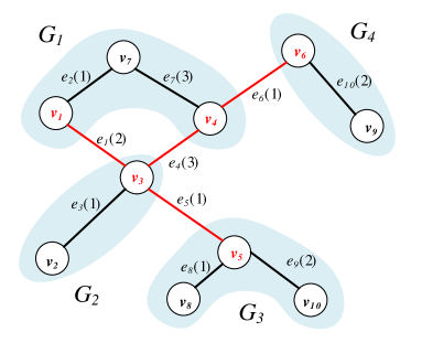
(a) Road Network Partition example. The red vertices represent the bridge vertices in each subgraph, while the red edges denote the cut edges connecting two disjoint subgraphs.

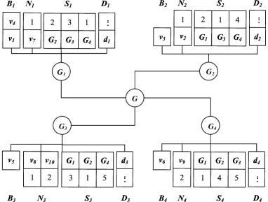
(b) Road Network Index example

Figure 1: An illustration example of road network indexing

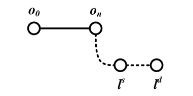
(a) The source insertion position $i$ and the destination insertion position $j$ are both after the $n$-th position (after finishing the existing trip schedule)

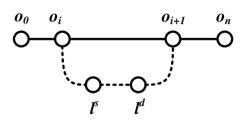
(b) $i$ and $j$ are consecutive and inserted before the $n$-th position

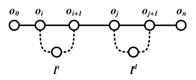
(c) $i$ and $j$ are not consecutive and inserted before the $n$-th position

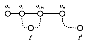
(d) $i$ is before the $n$-th position but $j$ is inserted after the $n$-th position

Figure 2: Four different ways the source and the destination points of a new rider can be inserted in an existing trip schedule

Density-based Partitioning.  We present a density-based partitioning approach which divides the road network $G$ into multiple subgraphs. The partition process follows two criteria: (1) Similar number of vertices: each subgraph maintains an approximately equal number of vertices such that the density distributions of the subgraphs are similar. (2) Minimal cut: an edge $e$ is considered as a cut if its two endpoints belong to two disjoint subgraphs. The number of cuts is minimal, so that the vertices in a subgraph are closely connected.

Given a road network $G=\langle V,E\rangle$ with a vertex set $V$ and an edge set $E$, a partition number $\tau$, $G$ is divided into a set of subgraphs $G_{1},G_{2},\ldots,G_{\tau}$, where each subgraph $G_{u}$ contains a subset of vertices $V_{u}$ and a subset of edges $E_{u}$ such that (1) $V_{1}\cup V_{2}\cup\ldots\cup V_{\tau}=V$, $E_{1}\cup E_{2}\cup\ldots\cup E_{\tau}\subseteq E$; (2) if $1\leq u,v\leq\tau$, and $u\neq v$, then $V_{u}\cap V_{v}=\emptyset$, $E_{u}\cap E_{v}=\emptyset$; (3) $|E_{1}|\approx|E_{2}|\approx\ldots\approx|E_{\tau}|$; (4) the number of edge cuts $|E|-\sum_{u=1}^{\tau}|E_{u}|$ is minimized.

The graph partitioning problem has been well-studied in the literature and is not the primary focus of this paper. Instead, we focus on how to define the distance bounds in order to reduce unnecessary shortest path distance computations. Thus we use a state-of-the-art method [41] to obtain the density based partitioning of the road network $G$.

Subgraph information.  After we obtain a set of disjoint subgraphs from $G$, we build our index by storing the following information for each subgraph $G_{i}$.

1. Bridge Vertex Set. If an edge $e$ is a cut, then each of its two endpoints is regarded as a bridge vertex. We store the set $B_{i}$ of the bridge vertices of each subgraph $G_{i}$.

2. Non-Bridge Vertex Set. Vertices not in $B_{i}$ of a subgraph $G_{i}$ are stored as a non-bridge vertex set $N_{i}$, i.e., $V_{i}\backslash B_{i}=N_{i}$. For each non-bridge vertex $u\in N_{i}$, we use $dis^{\downarrow}(u)$ to denote the lower bound distance of $u$, which is the shortest path distance to its nearest bridge vertex $v\in B_{i}$ in the same subgraph $G_{i}$.

3. Subgraph set. For each subgraph $G_{i}$, we store a list $S_{i}$ of the lower bound distances, one entry for each of the other subgraphs. Specifically, as the vertex of a subgraph is reachable from a vertex of another subgraph only through the bridge vertices, the lower bound distance $dis$$(G_{i},G_{j})$ is calculated with the following equation.

   $$\text{$dis$}(G_{i},G_{j})=\left\{\begin{matrix}0&\text{if }G_{i}=G_{j}\\ \min_{u,v}\text{$dis$}(u,v),\\ u\in B_{i},v\in B_{j}&\text{otherwise}\\ \end{matrix}\right.$$ (1)

4. Dispatched Driver Set. If the current location of a driver $d$ is situated in a subgraph $G_{i}$, then $d$ is stored in the dispatched driver set $D_{i}$.

4.3 Bounding Distance Estimations

Furthermore, we introduce two additional concepts on how to calculate the lower bound distance from a vertex to a subgraph (Definition 3) or another vertex (Definition 4).

Definition 3.

(Lower Bound Distance Between a Vertex and a Subgraph). Given a vertex $u$ which belongs to $G_{u}$ and a subgraph $G_{v}$, the lower bound distance $dist^{\downarrow}(u,G_{v})$ from $u$ to $G_{v}$ is defined as follows:

$$dis^{\downarrow}(u,G_{v})=\left\{\begin{matrix}0&\text{if }G_{u}=G_{v}\\ \text{$dis$}(G_{u},G_{v})&\text{if }G_{u}\neq G_{v},u\in B\\ \text{$dis$}(G_{u},G_{v})+dis^{\downarrow}(u)&\text{if }G_{u}\neq G_{v},u\notin B\\ \end{matrix}\right.$$ (2)

Definition 4.

(Lower Bound Distance Between Two Vertices). Given a vertex $u$ which belongs to $G_{u}$ and a vertex $v$ which is located at $G_{v}$, the lower bound distance $dist^{\downarrow}(u,v)$ is defined as follows:

$$\small dis^{\downarrow}(u,v)=\left\{\begin{matrix}0&\text{if }G_{u}=G_{v}\\ \text{$dis$}(G_{u},G_{v})&\text{if }G_{u}\neq G_{v},u\in B_{u},v\in B_{v}\\ \text{$dis$}(G_{u},G_{v})+dis^{\downarrow}(u)&\text{if }G_{u}\neq G_{v},u\notin B_{u},v\in B_{v}\\ \text{$dis$}(G_{u},G_{v})+dis^{\downarrow}(v)&\text{if }G_{u}\neq G_{v},u\in B_{u},v\notin B_{v}\\ \text{$dis$}(G_{u},G_{v})+dis^{\downarrow}(u)\\ +dis^{\downarrow}(v)&\text{otherwise}\\ \end{matrix}\right.$$ (3)

In our implementation, we construct the road network index offline and compute $dis^{\downarrow}(u,G_{v})$ or $dis^{\downarrow}(u,v)$ online. The index structure is memory resident, which includes $dis$$(G_{u},G_{v})$ and $dis^{\downarrow}(u)$ information. Therefore, $dis^{\downarrow}(u,G_{v})$ (or $dis^{\downarrow}(u,v)$) can be computed using Eq. 2 (or Eq. 3) in $O(1)$ time complexity.

Example 1.

A road network partitioning example is depicted in Fig. 1a. There are ten vertices and ten edges in the graph, and they are divided into four subgraphs: $G_{1}$, $G_{2}$, $G_{3}$, and $G_{4}$. The values in parenthesis after each edge denote the distance. The red vertices represent the bridge vertices in each subgraph, while the red edges denote the cut edges connecting two disjoint subgraphs. E.g., $e_{1}$ is a cut because it connects two disjoint subgraphs $G_{1}$ and $G_{2}$. $v_{1}$ and $v_{3}$ are two bridge vertices because they are two endpoints of a cut $e_{1}$.

The corresponding road network index structure is illustrated in Fig. 1b. For a subgraph $G_{1}$, $B_{1}$ includes two bridge vertices: $v_{1}$ and $v_{4}$. There is one remaining non-bridge vertex $v_{7}$ which belongs to $N_{1}$. Then the lower bound distance $dis^{\downarrow}(v_{7})$ from $v_{7}$ to a bridge vertex in the same subgraph is $\min\{$$dis$$(v_{7},v_{1}),$$dis$$(v_{7},v_{4})\}=1$. Three subgraphs are connected with $G_{1}$ directly or indirectly through cut edges. The distance between $G_{1}$ and $G_{2}$ is $dis(G_{1},G_{2})=\min\{dis(v_{1},v_{3}),dis(v_{3},v_{4})\}=2$, and the distance between $G_{1}$ and $G_{4}$ is $dis(G_{1},G_{4})=\min\{dis(v_{4},v_{6})\}=1$.

The lower bound distance $dis^{\downarrow}(v_{7},G_{3})$ between $v_{7}$ and $G_{3}$ is $dis(G_{1},G_{3})+dis^{\downarrow}(v_{7})=3+1=4$. The lower bound distance $dis^{\downarrow}(v_{7},v_{9})$ between $v_{7}$ and $v_{9}$ is $dis(G_{1},G_{4})+dis^{\downarrow}(v_{7})+dis^{\downarrow}(v_{9})=1+1+2=4$.

5 Pruning-based Rider Request Insertion

In this section, we propose a rider insertion algorithm on top of several pruning rules to insert a new incoming rider request $r$ into an existing trip schedule of a driver $d$ efficiently, such that a customized utility function $U$ is minimized, i.e., $U_{df}$ (Eq. 6) for Distance-first algorithm and $U_{gr}$ (Eq. 8) for Greedy algorithm, respectively.

5.1 Problem Assumption

First, same as prior work [15, 10, 35], when receiving a new rider request, a driver maintains the original, unchanged trip schedule sequence. In other words, we do not reorder the current trip schedule to ensure a consistent user experience for riders already scheduled. For example, if a driver has been assigned to pick up $r_{1}$ first and then pick up $r_{2}$, then the pickup timestamp of $r_{1}$ should be no later than the pickup timestamp of $r_{2}$. Second, in contrast to restrictions commonly adopted in prior work [10, 30, 34, 36], where the number of rider requests served by each driver is never greater than two, we assume that more than two riders can be served as long as the seat capacity constraint is not violated, which improves the usability and scalability of the ridesharing system.

5.2 Approach Description

Given a set of drivers $D$ and a new rider $r$, we aim to find a matching driver and insert $l^{s}$ and $l^{d}$ of $r$ into a driver’s trip schedule. A straightforward approach can be applied as follows: (1) for each driver candidate $d$, we enumerate all possible insertion positions for $l^{s}$ and $l^{d}$ in $d$’s current trip schedule (its complexity is $O(n^{2})$, where $n$ is the number of points in the trip schedule); (2) for each possible insertion position pair $\langle i,j\rangle$, we check whether it violates the waiting and detour time constraints of both $r$ and the other riders who have been scheduled for $d$ ($O(n)$). Therefore, the total time consumption is $O(n^{3})$. As the insertion process is crucial to the overall efficiency, we now propose several new pruning strategies. Then we present our algorithm for rider insertion derived from these pruning rules.

Before presenting the pruning strategies, we would like to introduce how the rider request is inserted and a preliminary called the slack distance.

Suppose that $l^{s}$ and $l^{d}$ are inserted in the $i$-th and $j$-th location respectively, where $i\leq j$ must hold. There are four ways to insert them as shown in Fig. 2. To accelerate constraint violation checking, we borrow the idea of “slack time” [14, 18] and define “slack distance”.

Definition 5.

(Slack Distance). Given a trip schedule $tr=\langle o_{0},o_{1},o_{2},\ldots,o_{n}\rangle$ where $o_{0}$ is the driver’s current location, the slack distance $sd[k]$ (Eq. 4) is defined as the minimal surplus distance to serve new riders inserted before the $k$-th position in $tr$. The surplus distance w.r.t. a particular point $o_{x}$ ($k\leq x\leq n$) after the $k$-th position is discussed as follows:

(1) If $o_{x}$ is a source point ($l_{x}^{s}$) of a rider request $r_{x}$, our only concern is whether the waiting time constraint $w_{x}$ will be violated. The actual pickup distance of $r_{x}$ from the driver’s current location is $dis_{a}(o_{0},o_{x})$, following the trip schedule. In the worst case, $r_{x}$ is picked up just within $w_{x}$. Then the surplus distance generated by $o_{x}$ is $w_{x}-dis_{a}(o_{0},o_{x})$.

(2) If $o_{x}$ is a destination point ($l_{x}^{d}$) of a rider request $r_{x}$, the detour time constraint will be examined. Similarly, the actual drop-off distance is $dis_{a}(l_{x}^{s},l_{x}^{d})$ following the trip schedule from the source point $l_{x}^{s}$. The worst case is that $r_{x}$ is dropped off within the border of detour time constraint, which is $(1+\theta_{x})dis(l_{x}^{s},l_{x}^{d})$ from $l_{x}^{s}$. Then the surplus distance generated by $o_{x}$ is $(1+\theta_{x})dis(l_{x}^{s},l_{x}^{d})-dis_{a}(l_{x}^{s},l_{x}^{d})$.

Thus we define the slack distance $sd[k]$ as Eq. 4.

$$\text{$sd[k]$}=\left\{\begin{matrix}\min\{sd[k+1],w_{k}-\text{$dis_{a}$}(o_{0},o_{k})\}&\text{if $o_{k}$ is a source}\\ \min\{sd[k+1],(1+\theta_{k})\text{$dis$}(l_{k}^{s},l_{k}^{d})\\ -\text{$dis_{a}$}(l_{k}^{s},l_{k}^{d})\}&\text{otherwise}\end{matrix}\right.$$ (4)

The available seat capacity $cp[k]$ (Eq. 5) in the process of pick-up and drop-off along the trip schedule changes dynamically.

$$\text{$cp[k]$}=\left\{\begin{matrix}cp[k-1]-rn&\text{if it is a source point}\\ cp[k-1]+rn&\text{otherwise}\end{matrix}\right.$$ (5)

In addition, we use an auxiliary variable $\triangle d(o_{a},o_{b},o_{c})$ to indicate the incremental distance by inserting $o_{b}$ between $o_{a}$ and $o_{c}$, then $\triangle d(o_{a},o_{b},o_{c})=dis(o_{a},o_{b})+dis(o_{b},o_{c})-dis(o_{a},o_{c})$.

Example 2.

Given a driver $d=\langle id,l,4,tr\rangle$ already carrying a rider $r_{1}=\langle 0,l_{1}^{s},l_{1}^{d},1,3,0.4\rangle$, and the current trip schedule $tr=\langle l,l_{1}^{d}\rangle$. On the driver’s way to drop off $r_{1}$, $d$ receives a new rider request $r_{2}=\langle 1,l_{2}^{s},l_{2}^{d},2,5,0.6\rangle$, then there are three possible updated trip schedules $tr^{\prime}_{1}=\langle l,l_{2}^{s},l_{2}^{d},l_{1}^{d}\rangle$, $tr^{\prime}_{2}=\langle l,l_{1}^{d},l_{2}^{s},l_{2}^{d}\rangle$, and $tr^{\prime}_{3}=\langle l,l_{2}^{s},l_{1}^{d},l_{2}^{d}\rangle$. For $tr^{\prime}_{1}$, we need to check whether the detour time constraint of $r_{1}$ and the waiting time constraint of $r_{2}$ are violated. For $tr^{\prime}_{2}$, we need to check whether the waiting time constraint of $r_{2}$ is violated. For $tr^{\prime}_{3}$, we need to check whether the detour time constraint of $r_{1}$, the waiting time constraint and detour time constraint of $r_{2}$ are violated.

5.3 Pruning Rules

5.3.1 Pruning driver candidates

Based on our proposed index in Section 4, we can estimate the lower bound distance from a driver to a rider’s pickup point. According to the waiting time constraint, drivers outside this range can be filtered out.

Lemma 1.

Given a new rider $r$ and a subgraph $G_{v}$, if $dis^{\downarrow}(l^{s},G_{v})>w$, then the drivers who are located in $G_{v}$ can be safely pruned.

Proof.

The lower bound distance $dis^{\downarrow}(l^{s},v)$ between the rider’s source point $l^{s}$ and any vertex $v$ in $G_{v}$ is always greater than or equal to the lower bound distance $dis^{\downarrow}(l^{s},G_{v})$ from $l^{s}$ to $G_{v}$. Therefore, if $dis^{\downarrow}(l^{s},G_{v})>w$ holds, then $\forall v\in G_{v}$, $dis^{\downarrow}(l^{s},v)>w$ also holds. Thus, the drivers located at any vertex in $G_{v}$ cannot satisfy the waiting time constraint of the rider. ∎

Lemma 2.

Given a new rider $r$ and a driver $d$, if $dis^{\downarrow}(l^{s},l)>w$, then $d$ can be safely pruned.

Proof.

Since the shortest path distance $dis(l^{s},l)$ between the new rider’s source point and the driver’s current location is no less than the lower bound distance $dis^{\downarrow}(l^{s},l)$, we have $dis(l^{s},l)>w$. ∎

5.3.2 Pruning rider insertion positions

It is worth noting that the insertion of a new rider may violate the waiting or detour time constraint of riders already scheduled for a vehicle, thus we propose the following rules to reduce the insertion time examination.

Lemma 3.

Given a new rider $r$, a trip schedule $tr$ and a source point insertion position $i$, if $dis(l,o_{i})>w$, then the rider should be picked up before the $i$-th point.

Proof.

Since each vehicle travels following a trip schedule, we have $dis(l,l^{s})=dis(l,o_{i})+dis(o_{i},l^{s})$, which is not less than $dis(l,o_{i})$. Then we can get $dis(l,l^{s})>w$, which violates the waiting time constraint of $r$. ∎

Lemma 4.

Given a new rider $r$, a trip schedule $tr$ and a source point insertion position $i$ ($i<n$), if $dis^{\downarrow}(o_{i},l^{s})+dis^{\downarrow}(l^{s},o_{i+1})-dis(o_{i},o_{i+1})>sd[i+1]$, then the rider cannot be picked up at the $i$-th point.

Proof.

The incremental distance generated by picking up $l^{s}$ is $\triangle d(o_{i},l^{s},o_{i+1})$, which is no smaller than $dis^{\downarrow}(o_{i},l^{s})+dis^{\downarrow}(l^{s},o_{i+1})-dis(o_{i},o_{i+1})$. Thus, we obtain $\triangle d(o_{i},l^{s},o_{i+1})>sd[i+1]$, which implies that the incremental distance exceeds the maximal waiting or detour tolerance range of point(s) after the $i$-th point. ∎

Lemma 5.

Given a new rider $r$ whose source point $l^{s}$ is already inserted at the $i$-th position of a trip schedule $tr$, and a destination point insertion position $j$, if $i=j<n$ (i.e., the insertion position as shown in Fig. 2b) and $dis^{\downarrow}(o_{i},l^{s})+dis(l^{s},l^{d})+dis^{\downarrow}(l^{d},o_{i+1})-dis(o_{i},o_{i+1})>sd[j+1]$, then $l^{d}$ cannot be inserted at the $j$-th point.

Proof.

Similar to Lemma 4, the additional distance as a result of inserting $l^{s}$ and $l^{d}$ is $dis(o_{i},l^{s})+dis(l^{s},l^{d})+dis(l^{d},o_{i+1})-dis(o_{i},o_{i+1})$, which is not less than $dis^{\downarrow}(o_{i},l^{s})+dis(l^{s},l^{d})+dis^{\downarrow}(l^{d},o_{i+1})-dis(o_{i},o_{i+1})$. Then the additional distance is greater than $sd[j+1]$, which violates the waiting or detour time constraint of the point(s) after the $j$-th point. ∎

Lemma 6.

Given a new rider $r$ whose source point $l^{s}$ is already inserted at the $i$-th position of a trip schedule $tr$, and a destination point insertion position $j$, if $i<j<n$ (i.e., the insertion position as shown in Fig. 2c) and $\triangle d(o_{i},l^{s},o_{i+1})+dis^{\downarrow}(o_{j},l^{d})+dis^{\downarrow}(l^{d},o_{j+1})-dis(o_{j},o_{j+1})>sd[j+1]$, then $l^{d}$ cannot be inserted at the $j$-th point.

Proof.

The incremental distance generated by dropping off $r$ at $l^{d}$ is $\triangle d(o_{j},l^{d},o_{j+1})$, which is no smaller than $dis^{\downarrow}(o_{j},l^{d})+dis^{\downarrow}(l^{d},o_{j+1})-dis(o_{j},o_{j+1})$. Then $\triangle d(o_{i},l^{s},o_{i+1})+\triangle d(o_{j},l^{d},o_{j+1})>sd[j+1]$, which violates the waiting or detour time constraint of point(s) after the $j$-th position. ∎

Lemma 7.

Given a new rider $r$, a trip schedule $tr$, and two insertion positions $i$ and $j$, if $i<j$ and $dis^{\downarrow}(l^{s},o_{i+1})+dis(o_{i+1},o_{j})+dis^{\downarrow}(o_{j},l^{d})>(1+\theta)dis(l^{s},l^{d})$, then such two insertion positions for $l^{s}$ and $l^{d}$ can be pruned.

Proof.

The actual travel distance $dis_{a}(l^{s},l^{d})$ from $l^{s}$ to $l^{d}$ is $dis(l^{s},o_{i+1})+dis(o_{i+1},o_{j})+dis(o_{j},l^{d})$, which is not less than $dis^{\downarrow}(l^{s},o_{i+1})+dis(o_{i+1},o_{j})+dis^{\downarrow}$($o_{j},l^{d})$. Then we can obtain that $dis_{a}(l^{s},l^{d})>(1+\theta)dis(l^{s},l^{d})$, which violates the detour time constraint of $r$. ∎

Lemma 8.

Given a new rider $r$, a trip schedule $tr$, and two insertion positions $i$ and $j$, $\forall k$ ($i\leq k\leq j$), if $rn>cp[k]$, then such two insertion positions for $l^{s}$ and $l^{d}$ can be pruned.

Proof.

It can be easily proved by the capacity constraint. ∎

In practice, we use the lower-bound distance to execute the pruning rules. If a possible insertion cannot be pruned, we use the true distance as a further check, which can guarantee the correctness of the pruning operation.

0:  a driver $d$ with a trip schedule $tr$$\langle o_{0},o_{1},\dots,o_{n}\rangle$, a new rider request $r$, a utility function $U$ 0:  return the utility value if $r$ can be served by $d$; Otherwise, return $-1$. 1:  $\mathscr{U}$$\leftarrow-1$, $\mathscr{U}^{*}$$\leftarrow\infty$ 2:  for $i\leftarrow 0$ to $n$ do 3:     if $cp[i]\geq rn$ or $dis$($l$,$o_{i}$)$\leq w$ then // Lemma 3 and 8 4:        if $i\geq n$ and $dis^{\downarrow}$($o_{i}$,$l^{s}$)+$dis^{\downarrow}$($l^{s}$,$o_{i+1}$)-$dis$($o_{i}$,$o_{i+1}$) $\geq sd[i+1]$ then // Lemma 4 5:           for $j\leftarrow i$ to $n$ do 6:              if $cp[j]\geq rn$ then // Lemma 8 7:                 if $j\textless n$ then 8:                    if $i$ = $j$ then 9:                       if $dis^{\downarrow}$($o_{i}$,$l^{s}$)+$dis$($l^{s}$,$l^{d}$)+$dis^{\downarrow}$($l^{d}$,$o_{i+1}$) $-$$dis$($o_{i}$, $o_{i+1}$)$\textgreater sd[j+1]$ then // Lemma 5 10:                          continue 11:                    else 12:                       if $\triangle d$($o_{i}$,$l^{s}$,$o_{i+1}$)+$dis^{\downarrow}$($o_{j}$,$l^{d}$)+$dis^{\downarrow}$($l^{d}$, $o_{j+1}$)-$dis$( $o_{j}$,$o_{j+1}$)$\textgreater sd[j+1]$ or $dis^{\downarrow}$($l^{s}$,$o_{i+1}$)+$dis$($o_{i+1}$,$o_{j}$)+$dis^{\downarrow}$($o_{j}$,$l^{d}$)$\textgreater$ ($1$+$\theta$)$dis$($l^{s}$,$l^{d}$) then // Lemma 6 and 7 13:                          continue 14:                 $\mathscr{U}$$\leftarrow$ compute the utility value using $U$ 15:                 if  $\mathscr{U}$$\textless$ $\mathscr{U}^{*}$ then 16:                    $\mathscr{U}^{*}$$\leftarrow$ $\mathscr{U}$ 17:  return  $\mathscr{U}^{*}$

Algorithm 1 RiderInsertion ($d$, $r$, $U$)

5.4 Algorithm Sketch

The pseudocode for the rider insertion algorithm is shown in Algo. 1. We initialize two local variables: $\mathscr{U}$ to record the utility value found each time, and the best utility value $\mathscr{U}^{*}$ found so far (line 1), where a lower value denotes better utility. The pruning rules are first executed for the pickup point $l^{s}$. We examine whether the vacant vehicle capacity is sufficient to hold the riders, and that the driver is close enough to provide the ridesharing service (line 3). If the conditions hold for the $i$-th position, then we check whether the detour distance will exceed the slack distance of the following points starting from the $i$-th position.

If all of the conditions are satisfied, we continue to check the destination point insertion (line 5). Otherwise, the source point is not added at the $i$-th position. Similarly, we check whether the current capacity is sufficient (line 6). Since the sequence between $i$ and $j$ leads to a different detour distance, two cases are possible: $i=j$ (i.e., the source and the destination are added to consecutive positions, shown in Fig. 2a and Fig. 2b) and $i<j$ (i.e., the positions are not consecutive, as shown in Fig. 2c and Fig. 2d). If $i=j$, we compute the incremental distance generated by $l^{s}$ and $l^{d}$, then judge whether it is greater than the slack distance of the following points after the $i$-th position (line 9). If $i<j$, besides checking whether the incremental distance generated by $l^{s}$ and $l^{d}$ is larger than the slack distance, we also need to check whether the detour time constraint of $r$ is violated (line 12). If the current utility value obtained is better than the current optimal value $\mathscr{U}^{*}$ found, we update $\mathscr{U}^{*}$ (line 16).

Time complexity analysis. The two nested loops (line 2 and 5), each iterating over $n$ points takes $O(n^{2})$ total time. The examination for constraint violations (line 3, 4, 6, 9, and 12) only takes $O(1)$. Calculating the utility function value $\mathscr{U}$ (line 14) also takes $O(1)$, which will be explained later according to different utility functions $U$. In our method, we use a fast hub-based labeling algorithm [40] to answer the shortest path distance query. First, a hub label index is constructed in advance by assigning each vertex $v$ (considered as a “hub indicator”) a hub label which is a collection of pairs ($u$, $dis$($v$, $u$)) where $u\in V$. Then given a shortest path query ($s$, $t$), the algorithm considers all common vertices in the hub labels of $s$ and $t$. Therefore, the shortest path distance from $s$ to $t$ depends on the sizes of the hub label sets. We assume that the time complexity is $O(\Omega)$, where $\Omega$ indicates the average label size of all label sets [42]. Therefore, the total time complexity is $O(n^{2}\Omega)$.

6 Matching-based Algorithm

In this section, we introduce two heuristic algorithms to bilaterally match a set of drivers and rider requests. Furthermore, we describe the insertion/update process for dynamic ridesharing.

6.1 Distance-first Algorithm

The Distance-first algorithm is executed in the following way: (1) we choose an unserved rider request $r$ with the earliest submission time from $R$, and perform the pruning-based insertion algorithm (Algo. 1) to find a driver $d$ with minimal additional distance. (2) If a driver $d$ can be found to match $r$, then the pair $(r,d)$ is joined and added to the final matching result.

The Distance-first algorithm has two important aspects. First, a matching for a single rider insertion is made whenever the constraints are not violated, even if the effectiveness is relatively low. Second, if multiple drivers are available to provide a ridesharing service, the Distance-first algorithm always chooses the one with the minimal additional distance. Thus, we define the optimization utility function $U_{df}$ as the additional distance $AD$.

$$\text{$U_{df}$}=AD$$ (6)

Based on the insertion option used (Fig. 2), we calculate $AD$ in Eq. 7. As the distance $dis(o_{0},o_{k})$ from a driver’s location to any existing point in $tr$ is already calculated and stored, the computation of $AD$ only takes $O(1)$ if the trip schedule $tr$ and two insertion positions are given. Specifically, $AD$ is calculated as:

$$AD=\left\{\begin{matrix}\text{$dis$}(o_{n},\text{$l^{s}$})+\text{$dis$}(\text{$l^{s}$},\text{$l^{d}$})&\text{if }i=j=n\\ \text{$dis$}(o_{i},\text{$l^{s}$})+\text{$dis$}(\text{$l^{s}$},\text{$l^{d}$})+\text{$dis$}(\text{$l^{d}$},o_{i+1})\\ -\text{$dis$}(o_{i},o_{i+1})&\text{if $i=j<n$}\\ \text{$\triangle d$}(o_{i},\text{$l^{s}$},o_{i+1})+\text{$\triangle d$}(o_{j},\text{$l^{d}$},o_{j+1})&\text{if $i<j<n$}\\ \text{$\triangle d$}(o_{i},\text{$l^{s}$},o_{i+1})+\text{$dis$}(o_{n},\text{$l^{d}$})&\text{otherwise}\\ \end{matrix}\right.$$ (7)

The pseudocode of the Distance-first method is illustrated in Algo. 2, which has two main phases: Filter and Refine. We initialize an empty set $L$ to store the current valid driver-rider pairs (line 1).

In the Filter phase (lines 2-7), for each rider we prune out ineligible driver candidates who violate the waiting time constraint. Specifically, for each rider $r_{j}$, we maintain a driver candidate list $D_{j}$ to store the drivers who can possibly serve $r_{j}$. We first prune the subgraphs from which it is impossible for a driver to serve $r_{j}$ (line 4). Then we further prune the drivers using a tighter bound, which is the lower bound distance between the driver’s location and the rider’s pickup point (line 6). The remaining drivers are inserted into $D_{j}$ as candidates.

In the Refine phase, the retained driver candidates are considered in the driver-rider matching process. We select one unserved rider with the earliest submission time (line 9) and find a suitable driver with minimal additional distance. In the for loop (lines 12-15), for each driver in $D_{j}$, we examine the feasibility by using Algo. 1 (line 13) and choose the one with the smallest additional distance (line 15). If a driver that can satisfy all the requirements is found, then $r_{j}$ is added to the corresponding trip schedule (line 17).

Time complexity analysis. In the Filter phase, the two nested iterations (line 2 and 5) takes $O(\tau|R||D_{u}|)$. The time complexity of the Refine phase is $O(|R||D_{u}|n^{2}\Omega)$. Therefore, the total time complexity is $O(\tau|R||D_{u}|+|R||D_{u}|n^{2}\Omega)$.

0:  a driver set $D$, a rider request set $R$ 0:  an assigned driver-rider pair list $L$; 1:  $L\leftarrow\emptyset$; 2:  for $G_{u}\in G$  do 3:     for $r_{j}$$\in R$  do 4:        if $dis^{\downarrow}($$r_{j}$.$l^{s}$$,G_{u})\leq$$r_{j}$.$w$ then // Lemma 1 5:           for $d_{i}$$\in G_{u}.D_{u}$  do 6:              if $dis^{\downarrow}$($r_{j}$.$l^{s}$,$d_{i}$.$l$)$\leq$$r_{j}$.$w$ then // Lemma 2 7:                 $D_{j}.push($$d_{i}$) 8:  while $R\neq\emptyset$ do 9:     choose one rider $r_{j}$ with the earliest submission time 10:     $R.pop($$r_{j}$$)$ 11:     $d\leftarrow NIL$, $AD_{i,j}\leftarrow-1$, $AD_{i,j}^{*}\leftarrow\infty$ 12:     for $d_{i}$ in $D_{j}$ do 13:        $AD_{i,j}\leftarrow$ RiderInsertion($d_{i}$, $r_{j}$, $U_{df}$) 14:        if $AD_{i,j}\textless AD_{i,j}^{*}$ then 15:           $AD_{i,j}^{*}\leftarrow AD_{i,j}$, $d\leftarrow$ $d_{i}$ 16:     if $d\neq NIL$ then 17:        insert rider $r_{j}$ to the current trip schedule of $d$ 18:        $L.push(d,$$r_{j}$$)$ 19:  return  $L$

Algorithm 2 The Distance-first Algorithm

6.2 Greedy Algorithm

The drawback of the Distance-first algorithm is that the rider request with the earliest submission time is selected in each iteration, which neglects the served rate. Therefore, we propose a Greedy algorithm in Algo. 3 to deal with our dual-objective problem: maximize the served rate and minimize the additional distance.

The Filter phase in Greedy is similar to that in Distance-first. However, in the Refine phase, we adopt a dispatch strategy by allocating the rider to the driver that results in the best utility gain (i.e., minimum utility value) locally each time, until there is no remaining driver-rider pair to refine. Since we want to make more riders happy, where the served riders can have less additional distance, we use a utility function to represent the average additional distance of the served riders. Then if $r_{j}$ is served by $d_{i}$, the utility function $U_{gr}$ is defined as:

$$\text{$U_{gr}$}=\frac{AD}{\text{$r_{j}$}.rn}$$ (8)

A rider request attached with more riders ($r_{j}.rn\textgreater 1$) is more favoured according to our utility gain (Eq. 8). For example, if a rider makes a ridesharing request with a friend, they tend to have the same source and destination point, which implies that the detour distance and waiting time can be reduced or even avoided (if not shared with other riders). On the contrary, if two separate requests are served by a driver, it is imperative for us to coordinate the dispatch permutation sequence and guarantee each of them is satisfied. We expect that $U$ is minimized as much as possible, i.e., more riders are served with less detour distance.

0:  a driver set $D$, a rider request set $R$ 0:  assigned driver-rider pair list $L$; 1:  $P\leftarrow$ a min-priority queue, $L\leftarrow\emptyset$ 2:  for $G_{u}\in G$  do 3:     for $r_{j}$$\in R$  do 4:        if $dis^{\downarrow}($$r_{j}$.$l^{s}$$,G_{u})\leq$$r_{j}$.$w$ then // Lemma 1 5:           for $d_{i}$$\in G_{u}.D_{u}$  do 6:              if $dis^{\downarrow}$($r_{j}$.$l^{s}$,$d_{i}$.$l$)$\leq$$r_{j}$.$w$ then // Lemma 2 7:                 $\mathscr{U}_{i,j}\leftarrow$ RiderInsertion($d_{i}$, $r_{j}$, $U_{gr}$) 8:                 if  $\mathscr{U}_{i,j}\neq\infty$ then 9:                    $P.push($$d_{i}$,$r_{j}$,$\mathscr{U}_{i,j}$) 10:  while $P\neq\emptyset$ do 11:     choose a pair $\langle d,r\rangle$ with minimal utility value from $P$ 12:     insert rider $r$ to the current trip schedule of $d$ 13:     $L.push(d,r)$ 14:     remove pairs $\langle*,r\rangle$ from $P$ 15:     for ($d$, $r_{j}$) $\in$ ($d$, *)  do 16:        if RiderInsertion($d$, $r_{j}$, $U_{gr}$) $\neq\infty$ then 17:           update the utility value of $\langle d,r_{j}\rangle$ in $P$ 18:        else 19:           remove the pair $\langle d,r_{j}\rangle$ from $P$ 20:  return  $L$

Algorithm 3 The Greedy Algorithm (GR)

The Greedy method is presented in Algo. 3. We initialize a min-priority queue $P$ to save the valid driver-rider pair candidates with their utility values, and an empty set $L$ to store our final result (line 1). In the Filter phase, we traverse each driver-rider pair to check whether they can be matched (lines 2-9). If the driver can carry the rider, then we will calculate its utility value (line 7) and push it into a pool $P$ (line  9). In the Refine phase, in each iteration we select the pair $\langle d,r\rangle$ with the smallest utility value greedily (line 11), we perform an insertion (line 12), and append the pair into our result list $L$ (line 13). Meanwhile, we remove all pairs related to $r$ from $P$ (line 14). For riders where $d$ was considered as a candidate, we check whether it is still valid to include them as a pair since the insertion of a new rider may influence the riders previously considered (lines 15-19). If $d$ is still feasible, we update the utility gain value for those riders (line 17). Otherwise, the driver-rider pair is removed from $P$ (line 19).

Time complexity analysis. Firstly, the time complexity to traverse each driver-rider pair to check whether they can be matched is $O(\tau|R||D_{u}|n^{2}\Omega)$. Each time we select a driver-rider pair with the lowest utility value greedily to insert ($O(|P|log|P|)$), remove those pairs related to $r$ from $P$ ($O(|P|)$) and then update the other influenced riders ($O(|P|n^{2}\Omega)$). Hence, the total time complexity is $O(\tau|R||D_{u}|n^{2}\Omega$+$|P|^{2}log|P|$+$|P|^{2}$+$|P|^{2}n^{2}\Omega)$.

6.3 Updating Process

After every $\triangle t$ time interval, we carry out the update process, including updating each non-empty driver’s current location, trip schedule and index information. If a driver is empty, then we assume that the state is static or inactive and unnecessary to be updated.

6.3.1 Update of the driver’s current location

We first obtain the trip schedule segment where the driver is located in a coarse-grained way, such as $(o_{k},o_{k+1})$ according to the actual completion distance $dis(o_{0},o_{k})$ of $o_{k}$ and the vehicle travel distance ($sp\times\triangle t$) within one timeslot, which has an $O(n)$ time complexity. Then we get the traversing edges set $E_{k}$ following the shortest path between $o_{k}$ and $o_{k+1}$, such as $e_{k1},e_{k2},\ldots,e_{kk}$. According to the remaining travel distance ($sp\times\triangle t-dis(o_{0},o_{k})$), we go through each edge in $E_{k}$ and pinpoint the edge $e_{d}$ where the driver is exactly, which has $O(|E_{k}|)$ time complexity. Finally, we choose an endpoint of $e_{d}$ as the current location of the driver approximately. In the worst case, the driver location update takes $O(n+|E_{k}|)$.

6.3.2 Trip schedule updates with slack distance

If the vehicle picks up new riders or drops off passengers on board, then the corresponding source or destination point should be removed from the original trip schedule. Meanwhile, we update the slack distance of each point $o_{k}$, which takes $O(n)$ time.

6.3.3 Update of the road network index information

Each subgraph $G_{i}$ maintains a list of vehicles which belong to $G_{i}$. If the driver moves from $G_{i}$ to another subgraph $G_{j}$, then it will be removed from $G_{i}$ and inserted into $G_{j}$. Given a vertex, it only takes $O(1)$ to obtain its situated subgraph. Thus updating the road network index takes $O(|D|)$ time.

7 Experiments

In this section, we perform an experimental evaluation on our proposed approaches. We first present the experimental settings in Section 7.1, and then validate the efficiency and effectiveness in Section 7.2 and Section 7.3.

7.1 Experimental Setting

Datasets. We conduct all experimental evaluations on a real Shanghai dataset [14], which includes road network data and taxi trips. The detailed statistical information is as follows:

• Road Network. There are $122{,}319$ vertices and $188{,}426$ edges in the Shanghai road network dataset [14]. Each vertex contains the latitude and longitude information. For each directly connected edge, the travel distance is given. The shortest path distance between any two vertices can be obtained by searching an undirected graph of the road network.

• Taxi Trip. In the Shanghai taxi trip dataset [14], there are $432{,}327$ taxi requests on May 29, 2009. Each taxi trip records the departure timestamp, pickup point, and dropoff point. Although we cannot estimate the exact request timestamp, we use the departure timestamp to simulate the request submission timestamp. The pickup and dropoff points are pre-mapped to the closest vertex on the road network. The initial location of a driver is randomly initialized as a vertex on the road network. For all initialized vehicles, we assume that there is no rider carried at the beginning.

Parameter settings. The key parameters of this work are listed in Table II, where the default values are in bold. For all experiments, a single parameter is varied while the rest are fixed to the default value. Note that speed $sp$ is a constant value set to 48 km/hr by default for convenience, but can be any value, as “speed” in this context is an average over the entire trip. Even though travel speed varies in reality, the travel time can be easily obtained if the speed and travel distance are known. Therefore, the scenario of varying speed is orthogonal to our problem.

Implementation. Experiments were conducted on an Intel(R) Xeon(R) E5-2690 CPU@2.60GHz processor with 256GB RAM. All algorithms were implemented in C++. The experiments are repeated $10$ times under each experimental setting and the average results are reported. For the “matching time” and “update time” metrics, we also report the results distribution. The size of our road network index is 1.85GB, and the index used in $DSA$ is 2GB.

Compared algorithms. The following methods were tested in our experiments:

• $DSA$ [11]. The primary baseline in our experiments, which has been shown to outperform another state-of-the-art approach recently [14].

• $DF$. The distance-first algorithm described in Section 6.1.

• $GR$. The greedy algorithm described in Section 6.2.

• $DF$+$P$. The distance-first algorithm described in Section 6.1 with our proposed pruning rules in Section 5.

• $GR$+$P$. The greedy algorithm described in Section 6.2 with our proposed pruning rules in Section 5.

Evaluation Metrics. We evaluate both efficiency and effectiveness under different parameter configurations.

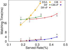
(a) Served rate

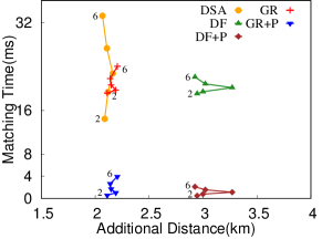
(b) Additional distance

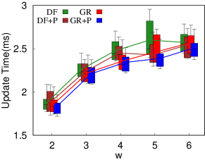
(c) Update time (The update time of $DSA$ is over $10$s, we omit it in the plot for better visualization)

Figure 3: Performance when varying the waiting time constraint $w$ from $2$ to $6$ minutes

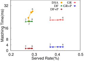
(a) Served rate

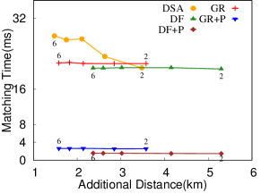
(b) Additional distance

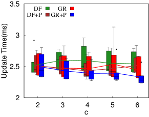
(c) Update time (The update time of $DSA$ is over $14$s, we omit it in the plot for better visualization)

Figure 4: Performance when varying the capacity $c$ from $2$ to $6$

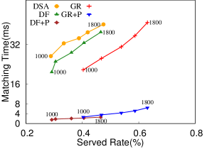
(a) Served rate

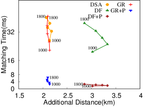
(b) Additional distance

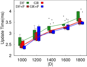
(c) Update time (The update time of $DSA$ is over $16$s, we omit it in the plot for better visualization)

Figure 5: Performance when varying the number of drivers $|D|$ from $1,000$ to $1,800$

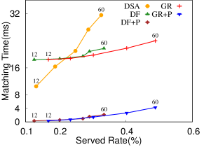
(a) Served rate

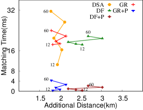
(b) Additional distance

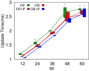
(c) Update time (The update time of $DSA$ is over $10$s, we omit it in the plot for better visualization)

Figure 6: Performance when varying the travel speed $sp$ from $12$ to $60$ km/hr

For the efficiency, we compare the matching time and update time, where matching time represents the average running time needed to match a driver to a single rider request, and the update time is the average running time required to amend a driver’s current trip schedule and update the underlying index. Note that we omit the measurement of the driver’s current location update because the driver’s location can be acquired from the GPS device in near realtime.

For the effectiveness, we compare the served rate and the additional distance. The served rate denotes the ratio of served rider number divided by the total rider number, and the additional distance is computed as the total additional distance divided by the number of served riders.

7.2 Experimental Results at Peak Travel Period

In this section, we sample $6{,}000$ orders in peak hours, because $DSA$ cannot process all the rider requests due to combinatorial time complexity (explained later). We show a series of efficiency and effectiveness trade-off graphs in order to better compare the performance differences between all of the algorithms. Beginning and end sweep values are shown for each line to make it easier to observe the performance trends for each algorithm. Note that $DF$ and $DF$+$P$ (or $GR$ and $GR$+$P$) maintain exactly the same values on “served rate” and “additional distance” metrics. As variants of certain algorithms have the similar efficiency profile, but a different one for effectiveness (thus the use of trade-off graphs). For the “update time” metric, we have added a very small point skew to the four lines to improve visualization.

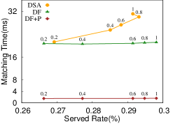
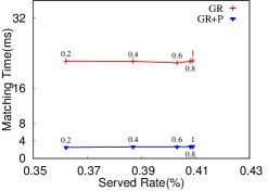
(a) Served rate

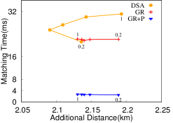
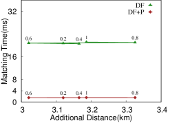
(b) Additional distance

Figure 7: Performance when varying the detour time constraint $\theta$ from $0.2$ to $1$ (The update time is shown in Fig. 9a)

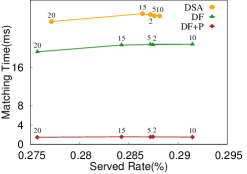
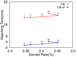
(a) Served rate

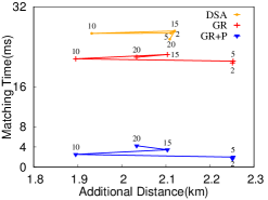
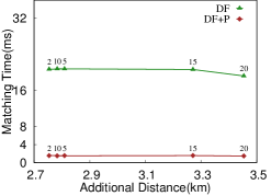
(b) Additional distance

Figure 8: Performance when varying the update time window $\triangle t$ from $2$ to $20$ seconds (The update time is shown in Fig. 9b)

Effect of the Waiting Time Constraint $w$. Fig. 3 shows the experimental results when varying $w$ from $2$ to $6$ minutes, where the first two sub-figures are trade-off graphs. With a larger waiting time, the served rates of all the algorithms increase because more driver candidates can satisfy the waiting time constraint. We observe that $GR$+$P$ consistently outperforms $DSA$ by approximately $10$% on served rate in Fig. 3a, while the average additional distance is increased slightly in Fig. 3b, which validates our proposed goal to serve more riders with less additional distance. $DSA$ and $DF$+$P$ maintain a similar served rate because both process rider requests in order of the submission time, regardless of the served rate. Moreover, it is reasonable that the additional distance of $DF$+$P$ may not keep a consistent decreasing trend in Fig. 3b. Increasing $w$ implies that more riders can share a trip and are also required to be served to their destinations. This could either increase or decrease the additional distance for the riders depending on multiple factors, such as request time, pickup, and drop off locations. In term of matching time, we observe that $DSA$ grows rapidly among all the algorithms in Fig. 3a because $DSA$ enumerates all the possible positions to insert $l^{s}$ and $l^{d}$ for a new rider, which requires $O(n!)$ time, where $n$ is the number of points in the trip schedule. With a larger $w$, more riders may share the vehicle such that $n$ is larger. In addition, the matching time of $GR$+$P$ is more than $10$ times faster than $GR$, which validates the efficiency of our proposed pruning rules. For the update time in Fig. 3c, our proposed methods are three orders-of-magnitude faster than $DSA$. Because $DSA$ must update two kinds of index structures: (1) each driver maintains a kinetic tree [14] to record a possible trip schedule for all unfinished requests assigned to each vehicle, which takes $O(|D|\times n!)$ [11]; (2) a grid index to store road network information and vehicles that are currently located or scheduled to enter each grid, which also has an $O(|D|\times n!)$ update time complexity [11]. In contrast, our methods only take $O(|D|\times n)$ to update the trip schedule for each vehicle, and $O(D)$ to update the road network index. Thus, we find that $DSA$ cannot finish updating with the allocated window of time ($10$ seconds), while our methods can. Although $GR$+$P$ performs worse than $DF$+$P$, it can have a higher served rate with less additional distance.

TABLE II: Parameter settings

Parameter	Setting
Waiting time constraint $w$ (min)	2, 3, 4, 5, 6
Detour time constraint $\theta$	0.2, 0.4, 0.6, 0.8, 1
Capacity of vehicle $c$	2, 3, 4, 5, 6
Number of vehicles $|D|$	1000,1200,1400,1600,1800
Size of the update timeslot $\triangle t$ (s)	2, 5, 10, 15, 20
Number of partitions $\tau$	500
Travel speed $sp$ (km/hr)	12, 24, 36, 48, 60

Effect of the Capacity $c$. Fig. 4 illustrates the results when varying the seat capacity from $2$ to $6$. With a larger $c$, all the algorithms have an increased served rate and lower additional distance because the vehicle can hold more riders. In term of matching time, $DF$ and $GR$ are relatively stable. When the capacity is small, most vehicles can be filtered by the capacity constraint, thus the matching time is lower. Our proposed methods have a similar update mechanism, and thus the update time is dramatically lower than $DSA$.

Effect of the Number of Drivers $|D|$. Fig. 5 plots the results when varying the number of drivers from $1{,}000$ to $1{,}800$. $GR$+$P$ still maintains the highest served rate relative to the other algorithms in Fig. 5a, while $GR$+$P$ can have a similar additional distance to $DSA$ as shown in Fig. 5b. In term of matching time, $DSA$, $DF$ and $GR$ maintain a steady growth trend as more drivers are available to serve a rider, which results in an increase in the number of driver verifications. Nevertheless, our proposed pruning rules can reduce the matching time of $DF$ and $GR$ by an order-of-magnitude in Fig. 5a.

Effect of the Travel Speed $sp$. Fig. 6 describes the results of varying the travel speed from $12$ to $60$ km/hr, which was also explored by Wang et al. [43] on speed variations during peak hour. We perform the experiments with different travel speeds in order to simulate diverse traffic conditions in peak hours that have a direct influence on the waiting time constraint. Obviously, the served rate of all the algorithms increases when the travel speed increases, because more rider requests can satisfy the waiting time constraint. When the travel speed is $12$ km/h, $GR$ (or $GR$+$P$) can achieve a $28.2\%$ improvement on served rate over $DSA$ from Fig. 6a, which corresponds to a slightly lower additional distance from Fig. 6b. This demonstrates that our methods can outperform the baseline consistently even under serious traffic congestion scenarios. From Fig. 6a, the matching time of $DSA$ keeps increasing with larger travel speed because more rider requests need to be considered for the assignment. In contrast, our methods are more robust.

Effect of the Detour Time Constraint $\theta$. Fig. 7 depicts the experimental results as $\theta$ is varied from $0.2$ to $1$. The served rate for all of the algorithms increases slightly with the change of $\theta$ in Fig. 7a, as the existing riders arranged in the trip schedule allow a greater detour distance to support more riders. Specifically, we can observe that $GR$+$P$ consistently has a higher served rate than $DSA$ or $DF$+$P$, while $GR$+$P$ degrades with the additional distance, and maintains a lower average additional distance with $DSA$ when $\theta=1$, as shown in Fig. 7b. In term of matching time, $DSA$ increases linearly in Fig. 7a because more riders can share the trip, which leads to more verified vehicles and longer matching time.

Effect of the Update Time Window $\triangle t$. Fig. 8 shows the results of varying the size of update time window from $2$ to $20$ seconds. The served rates of $DSA$, $DF$, and $DF$+$P$ are insensitive to the change of $\triangle t$, because they process each rider request in a first-come-first-serve manner. $GR$+$P$ has an increased serving rate with a larger $\triangle t$, because it can consider more rider requests within a time window and generate a better result to both maximize the served rate and minimize the additional distance. However, the served rates of all the algorithms drop when $\triangle t>15$, because we move the vehicle every $\triangle t$, and the seat capacity becomes saturated in the current timeslot. This also results in decreased matching times for most algorithms when $\triangle t>15$, while $GR$+$P$ increases slightly because it must still find the best possible matching.

Summary of the experimental results. $DF$+$P$ and $GR$+$P$ are improved versions of $DF$ and $GR$ whose pruning power consistently reduces the number of candidates considered in each time window. Pruning is more essential in high demand scenarios. In our experiments, $GR$+$P$ is preferable when the served rate exceeds $30\%$, and $DF$+$P$ is preferable when rider assignments must be executed in milliseconds.

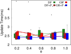
(a) Update time (The update time of $DSA$ is over $14$s, we omit it in the plot for better visualization)

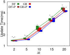
(b) Update time (The update time of $DSA$ is over $15$s, we omit it in the plot for better visualization)

Figure 9: The update time when varying $\theta$ and $\triangle t$

TABLE III: The performance of DF+P and GR+P in a Peak Hour simulation as $|D|$ varies

$|D|$	Served Rate		Additional Distance (km)		Matching Time (ms)		Update Time (ms)
	$DF$+$P$	$GR$+$P$	$DF$+$P$	$GR$+$P$	$DF$+$P$	$GR$+$P$	$DF$+$P$	$GR$+$P$
1000	0.175	0.192	2.314	1.806	2.878	13.962	13.191	13.495
3000	0.422	0.507	2.294	1.912	10.543	112.375	112.945	113.141
5000	0.601	0.711	2.270	2.038	12.177	116.870	15.633	15.527
7000	0.693	0.825	2.287	2.130	18.848	134.195	21.049	28.226
9000	0.770	0.884	2.275	2.175	25.875	148.375	27.566	34.476

7.3 Case Study

In order to show the scalability of our proposed methods on both efficiency and effectiveness in peak travel periods scenario, we adopt $DF$+$P$ and $GR$+$P$ to process $100,000$ orders in peak hours, where there are $20$ rider requests per second on average. We evaluate differing numbers of drivers in Table III to simulate a peak hour scenario, while other parameter values are held constant.

We could observe that $GR$+$P$ can obtain a $18.3$% higher served rate than $DF$+$P$ when $|D|=5000$, while requiring a smaller additional distance. In term of efficiency, $DF$+$P$ outperforms $GR$+$P$ because $GR$+$P$ requires more rider insertion algorithm invocations to find the minimal utility gain. Moreover, the update time of both $DF$+$P$ and $GR$+$P$ can be finished within the current timeslot.

7.4 Performance Bound

In addition, we perform a performance bound experiment to better observe the volatility of the algorithms explored in this work. As in prior work [44], we use Simulated Annealing ($SA$) to find the best solution under each time window for performance comparison.

Note that we have two objectives to achieve, thus we combine these two objectives into one single function by minimizing the utility function $U_{gr}$ (i.e., Eq. 8), where the smaller the utility value is, and the better the method will be. To be specific, we first generate an initial solution using $GR$+$P$. The initial solution could be chosen randomly without any constraint violation, but using $GR$+$P$ achieves a better result as verified in Section 7.2. Next, we perform $P$ perturbations for a number of $T$ temperatures. During each perturbation, we randomly select a rider request and then reassign it to a different driver, where the constraints will be further examined for the possible insertion. If a smaller utility value is obtained, then we insert the rider and update the driver’s trip schedule. Otherwise, if the utility value increases, then it is accepted with probability $p=\exp(-\frac{\Delta U}{T})$, where $\Delta U$ is the utility value difference before and after reassignment, and $T$ is the current temperature. The temperature is then reduced by a decay value $\delta*T$ proportional to the current temperature after every $P$ perturbations. The algorithm terminates when the temperature reaches zero. This alleviates the likelihood of converging to the same local optima repeatedly. If the temperature cool-down requires $t$ iterations, the time complexity of $SA$ is $O(tPn^{2}\Omega)$ including the quadratic cost $O(n^{2}\Omega)$ for each rider request insertion as discussed in Section 5. We omit the time complexity of finding the initial solution which only takes several milliseconds using $GR$+$P$ as it is not a factor (quantified below).

For all experiments, we use the default parameter setting from Table 2. The number of perturbations $P$ is $10{,}000$, the start temperature $T$ is set to $5$, and the decay parameter $\delta=0.001$. We process $1,000$ orders in five successive time windows. The experiments are repeated $10$ times and the average results are reported. The average matching time to process all the orders requires $28.3$ minutes ($1{,}698$ ms per rider request), while $GR$+$P$ only requires $3.253$ seconds ($3.253$ ms per rider request). For the effectiveness, the utility results of all methods are presented in Table IV. The effectiveness of $DF$ and $GR$ are excluded since they are the same as $DF$+$P$ and $GR$+$P$, respectively.

TABLE IV: Utility Scores for all Methods over Five Successive Time Windows.

	$1^{st}$	$2^{nd}$	$3^{rd}$	$4^{th}$	$5^{th}$
$DSA$	2.457	2.223	2.247	2.305	2.719
$DF$+$P$	2.575	2.580	2.484	2.537	2.869
$GR$+$P$	2.399	2.155	2.023	2.128	2.670
$SA$	2.157	1.947	1.889	1.951	2.281

8 Conclusion

In this paper, we proposed a variant of the dynamic ridesharing problem, which is a bilateral matching between a set of drivers and riders, to achieve two optimization objectives: maximize the served rate and minimize the total additional distance. In our problem, we mainly focus on the peak hour case, where the number of available drivers is insufficient to serve all of the rider requests. To speed up the matching process, we construct an index structure based on a partitioned road network and compute the lower bound distance between any two vertices on a road network. Furthermore, we propose several pruning rules on top of the lower bound distance estimation. Two heuristic algorithms are devised to solve the bilateral matching problem. Finally, we carry out an experimental study on a large-scale real dataset to show that our proposed algorithms have better efficiency and effectiveness than the state-of-the-art method for dynamic ridesharing. In the future, we plan to investigate how “fairness” can be applied to the driver-and-rider matching problem by defining a fair price mechanism for riders based on waiting time tolerance.

Hui Luo received the M.E. degree in computer science from Wuhan University, Hubei, China, in 2017. She is currently pursuing the Ph.D. degree at Computer Science and Information Technology, RMIT University, Melbourne, Australia. Her current research interests include data mining, intelligent transportation, and machine learning.

Zhifeng Bao received the Ph.D. degree in computer science from the National University of Singapore in 2011 as the winner of the Best PhD Thesis in school of computing. He is currently a senior lecturer with the RMIT University and leads the big data research group at RMIT. He is also an Honorary Fellow with University of Melbourne in Australia. His current research interests include data usability, spatial database, data integration, and data visualization.

Farhana M. Choudhury received the Ph.D. degree in computer science from RMIT University in 2017. She is currently a lecturer at The University of Melbourne. Her current research interests include spatial databases, data visualization, trajectory queries, and applying machine learning techniques to solve spatial problems.

J. Shane Culpepper received the Ph.D. degree at The University of Melbourne in 2008. He is currently a Vice-Chancellor’s Principal Research Fellow and Director of the Centre for Information Discovery and Data Analytics at RMIT University. His research interests include information retrieval, machine learning, text indexing, system evaluation, algorithm engineering, and spatial computing.

References

- [1] Didichuxing. [Online]. Available: https://www.didiglobal.com/
- [2] Uberpool. [Online]. Available: https://www.uber.com
- [3] L. Zhang, T. Hu, Y. Min, G. Wu, J. Zhang, P. Feng, P. Gong, and J. Ye, “A taxi order dispatch model based on combinatorial optimization,” in Proc. SIGKDD, 2017, pp. 2151–2159.
- [4] T. Teubner and C. M. Flath, “The economics of multi-hop ride sharing,” Business & Information Systems Engineering, vol. 57, no. 5, pp. 311–324, 2015.
- [5] J. Alonso-Mora, S. Samaranayake, A. Wallar, E. Frazzoli, and D. Rus, “On-demand high-capacity ride-sharing via dynamic trip-vehicle assignment,” Proc. National Academy of Sciences, vol. 114, no. 3, pp. 462–467, 2017.
- [6] Bureau of infrastructure, transport and regional economics. [Online]. Available: https://bitre.gov.au/publications/2015/yearbook_2015.aspx/
- [7] S. H. Jacobson and D. M. King, “Fuel saving and ridesharing in the us: Motivations, limitations, and opportunities,” Transportation Research Part D: Transport and Environment, vol. 14, no. 1, pp. 14–21, 2009.
- [8] Transforming the Mobility Industry: The Story of Didi. [Online]. Available: http://d20forum.org/wp-content/uploads/2017/12/11.50_Didi_Transforming-mobility_FINAL.pdf
- [9] A. Downs, Still stuck in traffic: coping with peak-hour traffic congestion, 2005. [Online]. Available: http://www.jstor.org/stable/10.7864/j.ctt1vjqprt
- [10] L. Zheng, L. Chen, and J. Ye, “Order dispatch in price-aware ridesharing,” PVLDB, vol. 11, no. 8, pp. 853–865, 2018.
- [11] L. Chen, Q. Zhong, X. Xiao, Y. Gao, P. Jin, and C. S. Jensen, “Price-and-time-aware dynamic ridesharing,” in Proc. ICDE, 2018, pp. 1061–1072.
- [12] N. Ta, G. Li, T. Zhao, J. Feng, H. Ma, and Z. Gong, “An efficient ride-sharing framework for maximizing shared route,” TKDE, vol. 30, no. 2, pp. 219–233, 2018.
- [13] S. Ma, Y. Zheng, and O. Wolfson, “T-share: A large-scale dynamic taxi ridesharing service,” in Proc. ICDE, 2013, pp. 410–421.
- [14] Y. Huang, F. Bastani, R. Jin, and X. S. Wang, “Large scale real-time ridesharing with service guarantee on road networks,” PVLDB, vol. 7, no. 14, pp. 2017–2028, 2014.
- [15] P. Cheng, H. Xin, and L. Chen, “Utility-aware ridesharing on road networks,” in Proc. SIGMOD, 2017, pp. 1197–1210.
- [16] X. Xing, T. Warden, T. Nicolai, and O. Herzog, “Smize: a spontaneous ride-sharing system for individual urban transit,” in Proc. MATES, 2009, pp. 165–176.
- [17] X. Fu, J. Huang, H. Lu, J. Xu, and Y. Li, “Top-k taxi recommendation in realtime social-aware ridesharing services,” in Proc. SSTD, 2017, pp. 221–241.
- [18] Y. Tong, Y. Zeng, Z. Zhou, L. Chen, J. Ye, and K. Xu, “A unified approach to route planning for shared mobility,” PVLDB, vol. 11, no. 11, pp. 1633–1646, 2018.
- [19] B. Cao, L. Alarabi, M. F. Mokbel, and A. Basalamah, “Sharek: A scalable dynamic ride sharing system,” in Proc. MDM, vol. 1, 2015, pp. 4–13.
- [20] S. Ma and O. Wolfson, “Analysis and evaluation of the slugging form of ridesharing,” in Proc. of SIGSPATIAL, 2013, pp. 64–73.
- [21] Y. Lin, W. Li, F. Qiu, and H. Xu, “Research on optimization of vehicle routing problem for ride-sharing taxi,” Procedia-Social and Behavioral Sciences, vol. 43, pp. 494–502, 2012.
- [22] S. Yan and C.-Y. Chen, “An optimization model and a solution algorithm for the many-to-many car pooling problem,” Annals of Operations Research, vol. 191, no. 1, pp. 37–71, 2011.
- [23] X. Wang, M. Dessouky, and F. Ordonez, “A pickup and delivery problem for ridesharing considering congestion,” Transportation letters, vol. 8, no. 5, pp. 259–269, 2016.
- [24] R. W. Hall and A. Qureshi, “Dynamic ride-sharing: Theory and practice,” Journal of Transportation Engineering, vol. 123, no. 4, pp. 308–315, 1997.
- [25] C.-C. Tao, “Dynamic taxi-sharing service using intelligent transportation system technologies,” in Proc. of WiCOM, 2007, pp. 3209–3212.
- [26] N. D. Chan and S. A. Shaheen, “Ridesharing in north america: Past, present, and future,” Transport Reviews, vol. 32, no. 1, pp. 93–112, 2012.
- [27] C. Morency, “The ambivalence of ridesharing,” Transportation, vol. 34, no. 2, pp. 239–253, 2007.
- [28] J.-F. Cordeau and G. Laporte, “The dial-a-ride problem: models and algorithms,” Annals of operations research, vol. 153, no. 1, pp. 29–46, 2007.
- [29] H. N. Psaraftis, “A dynamic programming solution to the single vehicle many-to-many immediate request dial-a-ride problem,” Transportation Science, vol. 14, no. 2, pp. 130–154, 1980.
- [30] X. Bei and S. Zhang, “Algorithms for trip-vehicle assignment in ride-sharing,” in Proc. AAAI, 2018.
- [31] N. Agatz, A. Erera, M. Savelsbergh, and X. Wang, “Optimization for dynamic ride-sharing: A review,” European Journal of Operational Research, vol. 223, no. 2, pp. 295–303, 2012.
- [32] M. Furuhata, M. Dessouky, F. Ordóñez, M.-E. Brunet, X. Wang, and S. Koenig, “Ridesharing: The state-of-the-art and future directions,” Transportation Research Part B: Methodological, vol. 57, pp. 28–46, 2013.
- [33] N. A. Agatz, A. L. Erera, M. W. Savelsbergh, and X. Wang, “Dynamic ride-sharing: A simulation study in metro atlanta,” Transportation Research Part B: Methodological, vol. 45, no. 9, pp. 1450–1464, 2011.
- [34] A. Kleiner, B. Nebel, and V. A. Ziparo, “A mechanism for dynamic ride sharing based on parallel auctions,” in Proc. IJCAI, vol. 11, 2011, pp. 266–272.
- [35] S. Ma, Y. Zheng, and O. Wolfson, “Real-time city-scale taxi ridesharing,” TKDE, vol. 27, no. 7, pp. 1782–1795, 2015.
- [36] X. Duan, C. Jin, X. Wang, A. Zhou, and K. Yue, “Real-time personalized taxi-sharing,” in Proc. DASFAA, 2016, pp. 451–465.
- [37] Y. Xu, Y. Tong, Y. Shi, Q. Tao, K. Xu, and W. Li, “An efficient insertion operator in dynamic ridesharing services,” in Proc. ICDE, 2019, pp. 1022–1033.
- [38] Y. Tong, J. She, B. Ding, L. Chen, T. Wo, and K. Xu, “Online minimum matching in real-time spatial data: experiments and analysis,” PVLDB, vol. 9, no. 12, pp. 1053–1064, 2016.
- [39] Y. Tong, J. She, B. Ding, L. Wang, and L. Chen, “Online mobile micro-task allocation in spatial crowdsourcing,” in Proc. ICDE, 2016, pp. 49–60.
- [40] I. Abraham, D. Delling, A. V. Goldberg, and R. F. Werneck, “A hub-based labeling algorithm for shortest paths in road networks,” in Proc. SEA, 2011, pp. 230–241.
- [41] G. Karypis and V. Kumar, “A fast and high quality multilevel scheme for partitioning irregular graphs,” SIAM Journal on Scientific Computing, vol. 20, no. 1, pp. 359–392, 1998.
- [42] Y. Li, M. L. Yiu, N. M. Kou et al., “An experimental study on hub labeling based shortest path algorithms,” PVLDB, vol. 11, no. 4, pp. 445–457, 2017.
- [43] X. Wang, T. Fan, W. Li, R. Yu, D. Bullock, B. Wu, and P. Tremont, “Speed variation during peak and off-peak hours on urban arterials in shanghai,” Transportation Research Part C: Emerging Technologies, vol. 67, pp. 84–94, 2016.
- [44] J. J. Pan, G. Li, and J. Hu, “Ridesharing: simulator, benchmark, and evaluation,” PVLDB, vol. 12, no. 10, pp. 1085–1098, 2019.