DySky: Dynamic Skyline Queries on Uncertain Graphs

Abstract.

Given a graph, and a set of query vertices (subset of the vertices), the dynamic skyline query problem returns a subset of data vertices (other than query vertices) which are not dominated by other data vertices based on certain distance measure. In this paper, we study the dynamic skyline query problem on uncertain graphs (DySky). The input to this problem is an uncertain graph, a subset of its nodes as query vertices, and the goal here is to return all the data vertices which are not dominated by others. We employ two distance measures in uncertain graphs, namely, Majority Distance, and Expected Distance. Our approach is broadly divided into three steps: Pruning, Distance Computation, and Skyline Vertex Set Generation. We implement the proposed methodology with three publicly available datasets and observe that it can find out skyline vertex set without taking much time even for million sized graphs if expected distance is concerned. Particularly, the pruning strategy reduces the computational time significantly.

1. Introduction

‘Skyline’ has emerged as an effective multi-criteria decision making operator and hence an extensively researched topic in data management community for almost two decades (Chomicki et al., 2013). Borzsony et al. (Borzsony et al., 2001) fist introduced this operator. Given a set of data points $D$, the skyline operator in it returns the subset of them that are not dominated by other data points present in the dataset. For any two points $d_{1}$ and $d_{2}$, we say that $d_{1}$ dominates $d_{2}$, if with respect to each dimension $d_{1}$ is not worse than $d_{2}$, however, strictly better in at least one dimension. Without loss of generality, in this study, we assume that lower value means better in all dimensions. This problem has been studied in the context of graph data as well (Zou et al., 2010; Zheng et al., 2014). In real-world scenarios, the relationship among agents are uncertain in nature and this uncertainty is caused due to several reasons noisy measurements, unknown values, explicit manipulations, etc. Hence, this kind of situations are modeled as an uncertain graph, where edges are marked with existence probabilities. In case of social networks, these probabilities signify the influence probability between two users, in case of computer networks these signify the successful packet transfer probability between two systems etc. Now, we report some recent literature on skyline query processing and analysis of uncertain graphs.

1.1. Related Work

After introduced by Borzsony et al. (Borzsony et al., 2001), skyline queries have been studied on different kinds of data, for different purposes, with different system architectures, such as road networks (Miao et al., 2018; Fu et al., 2017; Zhu et al., 2018), bi-criteria networks (Jiang et al., 2016; Ouyang et al., 2018), uncertain data (Zhou et al., 2015; Nguyen and Cao, 2015), incomplete data (Lee et al., 2016; Miao et al., 2016), streaming data (De Matteis et al., 2015; Liu et al., 2019), spatial data (Son et al., 2017), encrypted data (Liu et al., 2018b), knowledge graphs (Keles and Hose, 2019), wireless sensors networks (Wang et al., 2016); for route recommendations (Yawalkar and Ranu, 2019; Jiang and Du, 2018), finding perspective customers (Yin et al., 2018); resisting outliers (Jaudoin et al., 2017), favorite product queries (Zhou et al., 2016); with map reduce architecture (Park et al., 2017, 2015), multi-core architectures (De Matteis et al., 2016), cloud computing framework (Huang et al., 2018) and so on. Keeping the topic of this paper in our mind, here we elaborate the skyline query processing on probabilistic and uncertain data. He et al. (He et al., 2016) studied the skyline query on uncertain time series data and developed a two step methodology for to answer this probabilistically. Park et al. (Park et al., 2015) studied the skyline query processing on uncertain data and proposed parallel algorithms for computing the same using map reduce framework. Zhou et al. (Zhou et al., 2015) studied the skyline query processing over uncertain data in distributed environments. Le et al. (Le et al., 2016) studied the skyline queries on uncertain data to return the user specific relevant results without enumerating all possible worlds. Recently, there are several studies in this directions (Zeng et al., 2019; Liu et al., 2018a, 2019). However, to the best of our knowledge skyline query has not been studied yet in the context of uncertain graphs.

Due to different practical applications, in recent times analysis of uncertain graphs have emerged as an important research topic (Khan et al., 2018; Khan and Chen, 2015). Several problems have been studied such as clustering (Halim et al., 2017; Chen et al., 2015), embedding (Hu et al., 2017), subgraph search (Jin et al., 2011; Chen et al., 2015), structural pattern findings (Bonchi et al., 2014) and so an. Ke et al. (Ke et al., 2019b) studied the ‘budgeted reliability maximization problem’, where the goal is to add small number of edges to increase the reliability between a given pair of nodes. ke et al. (Ke et al., 2019a) recently studied the $s-t$ reliability problem which asks with how much probability a target node $t$ is reachable from a source node $s$ in a given uncertain graph. Chen et al. (Chen et al., 2018) studied the frequent pattern finding in uncertain graphs and for this problem enumeration-evaluation algorithm for this problem. Look into (Kassiano et al., 2016) for survey.

1.2. Our Contribution

In this paper, we propose the noble problem “dynamic skyline query on uncertain graphs”. Given an uncertain graph with a subset of vertices as query vartices, the goal of this problem is to obtain the subset of the data vertices that are not dominated by the other data vertices with respect to some distance measure from the query vertices. Particularly, we make the following contributions in this paper:

• We introduce the noble problem “Dynamic Skyline Queries on Uncertain Graph Problem” (DySky).

• We propose a solution methodology for this problem, which broadly divided into three steps, namely, pruning, distance computation and skyline vertex set generation.

• Proposed methodology has been implemented with three benchmark datasets and results show that the pruning strategy leads to less number of candidate nodes.

1.3. Organization

Rest of the paper is organized as follows: Section 2 describes required preliminary definitions and then define the problem formally. The proposed methodology has been described in Section 3. In Section 4 the experimental evaluations of the proposed methodology has been described. Section 5 draws conclusions and gives future directions.

2. Preliminaries and Problem Definition

In this section, we present required preliminary concepts and then define the dynamic skyline queries on uncertain graph problem formally. Initially, we start with a few basic definitions.

Definition 1 (Uncertain Graph).

We denote an uncertain graph by $\mathcal{G}(\mathcal{V},\mathcal{E},\mathcal{W},\mathcal{P})$, where $\mathcal{V}(\mathcal{G})=\{v_{1},v_{2},\ldots,v_{n}\}$ is the set of $n$ vertices, $\mathcal{E}(\mathcal{G})\subseteq\mathcal{V}(\mathcal{G})\times\mathcal{V}(\mathcal{G})$ is the set of $m$ edges, $\mathcal{W}$ is the distance function that assigns each edge to a positive real number, i.e., $\mathcal{W}:\mathcal{E}(\mathcal{G})\longrightarrow\mathbb{R}^{+}$, and $\mathcal{P}$ is the existence function that assigns each edge to a probability value, i.e., $\mathcal{P}:\mathcal{E}(\mathcal{G})\longrightarrow(0,1]$.

In our study, we consider only simple, finite, undirected, and weighted graphs. The number of nodes and edges of the graph $\mathcal{G}$ is denoted by $n$ and $m$, respectively. For an edge $e\in\mathcal{E}(\mathcal{G})$ its weight and existence probability is denoted by $\mathcal{W}(e)$ and $\mathcal{P}(e)$, respectively. In the literature, an uncertain graph is conceptualized and analyzed by the possible world model, which we define next.

Definition 2 (Possible World Semantics).

An uncertain graph $\mathcal{G}(\mathcal{V},\mathcal{E},\mathcal{W},\mathcal{P})$ can be conceptualized as the probability distribution over a set of deterministic graphs, which is called as the possible world of the uncertain graph, and denoted as $\mathcal{L}(\mathcal{G})$. Each $G(V,E,W)\in\mathcal{L}(\mathcal{G})$ is obtained from $\mathcal{G}$ by keeping all its vertices, keeping its edges with existing probability, and if an edge of $\mathcal{G}$ is also there in $G$, then $\mathcal{W}(e)=W(e)$. Now, the probability that the deterministic garph $G$ will be generated can be computed by the Equation 1.

(1) $$\mathcal{P}_{G\sqsubseteq\mathcal{G}}=\underset{e\in E(G)}{\prod}\mathcal{P}(e)\underset{e\in E(\mathcal{G})\setminus E(G)}{\prod}(1-\mathcal{P}(e))$$

In any deterministic graph $G$, its two vertices $v_{i}$ and $v_{j}$ are said to be reachable if there exist a path from between $v_{i}$ and $v_{j}$. However, in case of uncertain graphs, the reachability between any two given vertices can be defined in probabilistic way, which we call reliability.

Definition 3 (Reliability).

Given an undirected, uncertain graph $\mathcal{G}$, the reliability between its any two vertices $v_{i}$ and $v_{j}$ is defined as the probability that the vertices $v_{i}$ and $v_{j}$ can be reachable from each other. We denote the reliability between the vertices $v_{i}$ and $v_{j}$ by $\mathcal{R}^{\mathcal{G}}_{(v_{i}v_{j})}$ and defined by the following equation:

(2) $$\mathcal{R}^{\mathcal{G}}_{(v_{i}v_{j})}=\underset{G\in\mathcal{L}(\mathcal{G})}{\sum}I^{G}_{(v_{i}v_{j})}\mathcal{P}_{G\sqsubseteq\mathcal{G}}.$$

Here, $I^{G}_{(v_{i}v_{j})}$ is the boolean variable whose value is $1$ if $v_{i}$ and $v_{j}$ are connected in $G$ and $0$ otherwise.

In case of a deterministic weighted graph, distance between any two vertices is defined as the sum of individual edge weights constituting shortest path. However, in case of uncertain graphs distance between any two vertices can be defined in many ways. Here, we quote two of them that we use in our study.

Definition 4 (Majority Distance).

(Potamias et al., 2009) Given an uncertain graph $\mathcal{G}$ and its two vertices $v_{i},v_{j}\in V(\mathcal{G})$, its majority distance is denoted by $dist_{md}(v_{i},v_{j})$ and defined as the most probable shortest path distance. Mathematically, it can be given by the following equation.

(3) $$dist_{md}(v_{i},v_{j})=\underset{d}{argmax}\ p_{v_{i}v_{j}}(d)$$

where $p_{v_{i}v_{j}}$ is the shortest path distribution between the vertices $v_{i}$ and $v_{j}$ that gives probability value for every distance $d$.

(4) $$p_{v_{i}v_{j}}(d)=\underset{G|d_{G}(v_{i},v_{j})=d}{\sum}\mathcal{P}_{G\sqsubseteq\mathcal{G}}$$

Definition 5 (Expected Distance).

Given an uncertain graph $\mathcal{G}$ and its two vertices $v_{i},v_{j}\in V(\mathcal{G})$, let $P^{l}_{(v_{i}v_{j})}$ denotes the set of paths upto length $l$. For each path $p_{k}\in P^{l}_{(v_{i}v_{j})}$, the path probability is defined as

(5) $$\mathbb{P}(p_{k})=\frac{\prod_{e\in p_{k}}\mathcal{P}(e)}{\sum_{p_{j}\in P^{l}_{(v_{i}v_{j})}}\prod_{e\in p_{j}}\mathcal{P}(e)}$$

Expected distance between $v_{i}$ and $v_{j}$ is defined as the

(6) $$dist_{E}(v_{i},v_{j})=\underset{p_{k}\in P^{l}_{(v_{i}v_{j})}}{\sum}dist(p_{k}).\mathbb{P}(p_{k})$$

For any $p\in\mathbb{Z}^{+}$, $[p]$ denotes the set $\{1,2,\dots,p\}$. Given a set of $2$ or more dimensional data points $\mathcal{D}$, the problem of skyline query computation asks to find out the data points that are not dominated by any other data points in $\mathcal{D}$, which is formally defined in Definition 6.

Definition 6 (Skyline Query).

Given a set of $p$ dimensional data points $\mathcal{D}=\{d_{1},d_{2},\ldots,d_{|\mathcal{D}|}\}$, we say that $d_{i}$ dominates $d_{j}$, if for all $k\in[p]$, $d_{i}(k)\leq d_{j}(k)$ and there exist atleast one $k\in[p]$ such that $d_{i}(k)<d_{j}(k)$. Skyline of the dataset $\mathcal{D}$ is the subset of the data points that are not dominated by any of the data points in $\mathcal{D}$.

Since past one decade or so, skyline queries have been studied extensively (Zou et al., 2010; Khan et al., 2012) in graphs as well, which we define next.

Definition 7 (Skyline Query in Graphs).

Given a graph $G(V,E)$, and a subset of vertices $\mathcal{Q}$ (called query vertices), for any two data vertices (vertices that are not query vertices, i.e., $V(G)\setminus\mathcal{Q}$) $v_{i}$ and $v_{j}$, we say $v_{i}$ dominates $v_{j}$, if $\forall w\in\mathcal{Q}$, $dist(w,v_{i})\leq dist(w,v_{j})$ and $\exists x\in\mathcal{S}$, such that $dist(x,v_{i})<dist(x,v_{j})$. The skyline query asks to return data vertices that are not dominated by other data vertices.

Though, the skyline query problem has been studied in the context of probabilistic data (Atallah and Qi, 2009; Le et al., 2016; Zhang et al., 2019), to the best of our knowledge this problem has not been studied in the context of uncertain graphs. In this paper, we introduce the problem of finding the dynamic skyline queries on uncertain graphs (DySky), which is defined next.

Definition 8 (Dynamic Skyline Queries on Uncertain Graphs).

Given an uncertain graph $\mathcal{G}$, and a subset of vertices $\mathcal{Q}$ (called query vertices), the problem of dynamic skyline queries on uncertain graphs asks to find out the subset of the data vertices such that none of them are dominated by the other data vertices.

Figure 1 shows a toy example of an uncertain graph with its majority distance, expected distance, and shortest path distance (for deterministic version) tables, where the skyline vertices are marked in orange color. It is important to observe as the distance measure changes, the skyline vertex set is also getting changed. This motivates us to study the DySky Problem under two different distance measures.

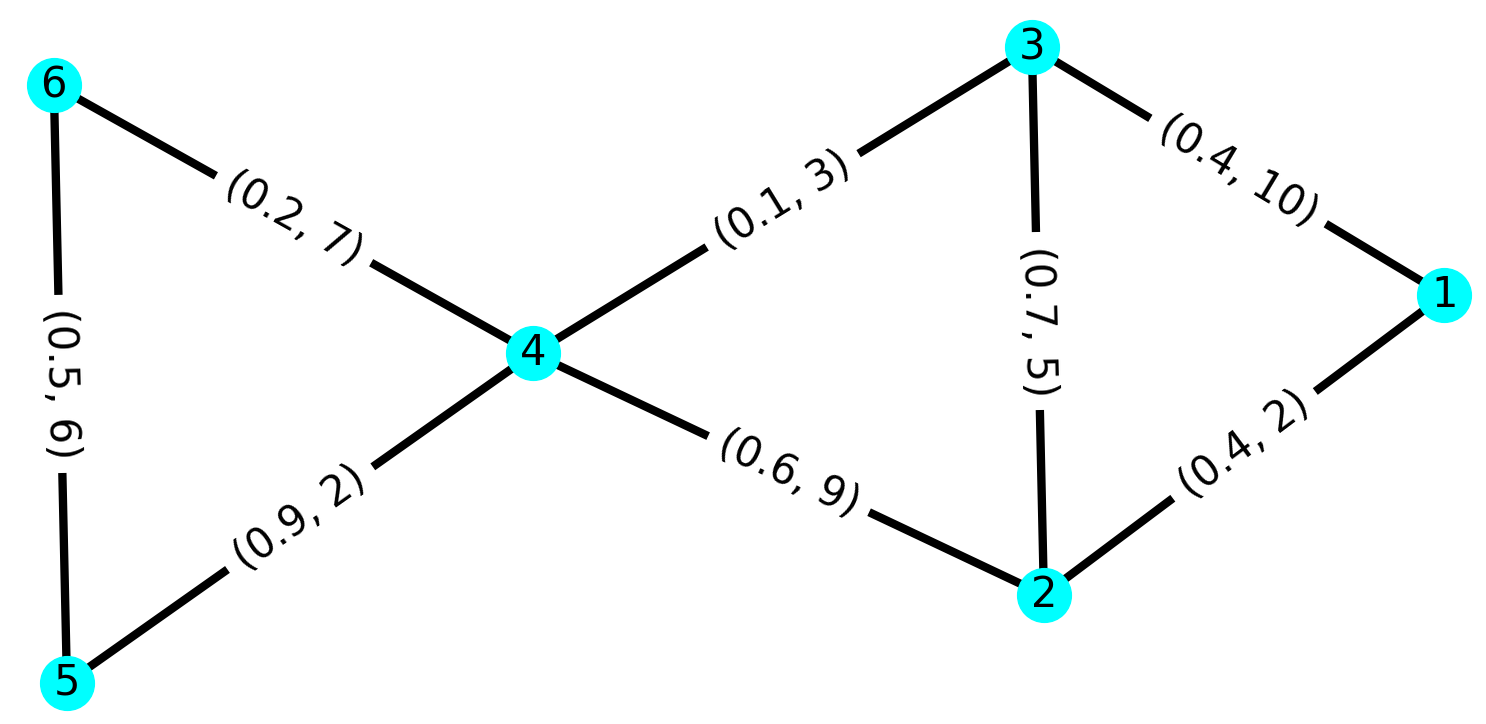
(a) An Uncertain Graph

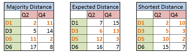
(b) Majority Distance (MD), Expected Distance,

and Shortest Path Distance (in deterministic version)

Figure 1. (a) An uncertain graph with $6$ vertices and $8$ edges. The vertices $2$ and $4$ are the Query Vertices (denoted as $Q2$ and $Q4$) and remaining are data vertices (i.e., $D1$, $D3$, $D5$, and $D6$). (b) Different distance tables between the query and data vertices. Skyline vertices in each cases are marked in Orange.

3. Proposed Methodology

Now, we describe the proposed methodology for solving the DySky Problem. Initially, we start by describing an overview of it.

3.1. Overview

The proposed methodology is broadly divided into three steps:

• Step 1 (Pruning): In this step, a subset of the data vertices are returned as the candidate skyline vertices. This step comprises of two subsets. First, pruning is done by performing Breadth First Search (B.F.S., henceforth) from the query vertices and subsequently, pruning is done based on distance computation.

• Step 2 (Distance Computation): In this step, distance computation is done between the candidate skyline vertices and query vertices. As mentioned previously, in our study we have used majority distance and expected distance.

• Step 3 (Skyline Vertex Set Generation): Based on the previously computed distance, any existing skyline finding algorithm can be used to find out the actual skyline vertices. In our study, we have used the Block Nested Loop (BNL) Algorithm proposed by Borzsonyi et al. (Borzsony et al., 2001).

Next, we proceed towards representing the proposed methodology in an algorithmic form and its detailed analysis.

3.2. The Algorithm

Algorithm 1, 2, and 3 together constitute the proposed methodology for the DySky Problem. We describe the entire procedure in two subsections. First we start with describing the pruning step.

3.2.1. The Pruning Step

Algorithm 1 describes the B.F.S. and distance based pruning strategies, which takes the uncertain graph, the set of query vertices, and distance threshold as inputs and outputs the candidate skyline vertices. In B.F.S. pruning, from each of the query vertices, B.F.S. trees are constructed to check the connectivity. First, we create the dictionary $\mathcal{D}$. If a query vertex and data vertex is connected and the data vertex has the entry in the dictionary $\mathcal{D}$, the query vertex is included as a value corresponding to this key. Otherwise, a key corresponding to the data vertex is created and the query vertex is added as a value to this ‘key’. Now, the data vertices that are reachable from all the query vertices are kept as the candidate skyline vertices. Here, the B.F.S. pruning ends.

In reality, even if two vertices are connected by a path of large distance (i.e., more than certain threshold), reachability becomes costlier. Hence, to eliminate such vertices, we perform the distance-based pruning. For this purpose, distance between candidate skyline vertex and query vertex is computed. For a candidate skyline vertex, if there exist atleast one query vertex for which the computed distance value is more than the user defined threshold, the candidate skyline vertex set is updated by removing the candidate skyline vertex.

Data: Uncertain Graph $\mathcal{G}(\mathcal{V},\mathcal{E},\mathcal{W},\mathcal{P})$, The Set of Query Vertices $\mathcal{Q}\subseteq\mathcal{V}(\mathcal{G})$, Distance Threshold $T$

. Result: Candidate Skyline Vertices $\mathcal{CS}\subseteq\mathcal{V}(\mathcal{G})\setminus\mathcal{Q}$

1 $\text{Create Dictionary }\mathcal{D}$;

2 for $\text{All }u\in\mathcal{Q}$ do

3       for $\text{All }v\in V(\mathcal{G})\setminus\mathcal{Q}$ do

4             if Isconnected(uv) then

5                   if $v\in\mathcal{D}.Keys()$ then

6                         $\mathcal{D}[v].values()=\mathcal{D}[v].values()\cup\{u\}$

7                  else

8                         $\mathcal{D}.Create\_Key(v)$;

9                         $\mathcal{D}[v].Add\_Value(u)$

10                   end if

11                  

12             end if

13            

14       end for

15      

16 end for

17$\mathcal{CS}=\emptyset$;

18 for $\text{All }u\in\mathcal{D}.Keys()$ do

19       if $\mathcal{D}[u].Values()=\mathcal{Q}$ then

20             $\mathcal{CS}=\mathcal{CS}\cup\{u\}$;

21            

22       end if

23      

24 end for

25for $\text{All }v\in\mathcal{CS}$ do

26       for $\text{All }u\in\mathcal{Q}$ do

27             if $distance(uv)>T$ then

28                   $\mathcal{CS}=\mathcal{CS}\setminus\{v\}$;

29                  

30             end if

31            

32       end for

33      

34 end for

Algorithm 1 Step 1 (B.F.S and Distance based pruning)

Any pruning strategy to work correctly should guarantee that it does not remove any skyline vertex. Hence, we show that the Algorithm 1 is a correct pruning strategy in Lemma 1.

Lemma 1.

The proposed pruning strategy (Algorithm 1) is correct.

Proof.

Follows from the description. ∎

Now, we do an analysis for time and space requirement of Algorithm 1. Let $q$ be the number of query vertices, i.e., $|\mathcal{Q}|=q$. For creating the B.F.S. trees rooted at the query vertices requires $\mathcal{O}(q(m+n))$ time. The maximum number of values associated with a ‘key’ in the dictionary $\mathcal{D}$ is of $\mathcal{O}(q)$. Execution time from Line No. $3$ to $14$ and $16$ to $20$ requires $\mathcal{O}(q(n-q)^{2})$ and $\mathcal{O}((n-q)q^{2})$. Now, in distance-based pruning, the number of distance computations is $\mathcal{O}(q(n-q))$. Computing shortest path between two vertices in a weighted graph with positive edge weights requires $\mathcal{O}(m+n\log n)$ time. Hence, time requirement for distance-based pruning requires $\mathcal{O}(q(n-q)(m+n\log n))$ time. Total time requirement for Algorithm 1 is of $\mathcal{O}(q(m+n)+nq(n-q)+q(n-q)(m+n\log n))=\mathcal{O}(q(n-q)(m+n\log n))$. Extra space requirement of Algorithm 1 is to store the dictionary $\mathcal{D}$, which is of $\mathcal{O}(q(n-q))$, to store the candidate skyline vertices, which is of $\mathcal{O}(n-q)$, and to perform the B.F.S., which is of $\mathcal{O}(n)$. Hence, total space requirement of Algorithm 1 is of $\mathcal{O}(q(n-q))$. Lemma 2 describes the formal statement.

Lemma 2.

Time and space requirement of Algorithm 1 is of $\mathcal{O}(q(n-q)(m+n\log n))$ and $\mathcal{O}(q(n-q))$, respectively.

3.2.2. Distance Computation and Skyline Vertex Set Generation

Now, we describe Step $2$ and $3$ of our proposed methodology. It is important to observe that depending upon which distance measure is used (i.e., majority distance or expected distance) Step $2$ will be different. Algorithm 2 and 3 describes the last two steps for the majority distance and expected distance, respectively.

Data: Candidate Skyline Vertices $\mathcal{CS}$

. Result: The Skyline Vertex Set $\mathcal{S}$.

1 $\text{Generate }|\mathcal{R}|\text{ number of samples graphs}$ ;

2 $\text{Store the graph probabilities in }\mathcal{P}_{G}[1\dots|\mathcal{R}|]$;

3 $\text{Create\_Matrix }\mathcal{M}\in\mathbb{R}^{|\mathcal{CS}|\times|\mathcal{Q}|}$;

4 for $\text{All }u\in\mathcal{CS}$ do

5       for $\text{All }v\in\mathcal{Q}$ do

6             Create dictionary $Temp$;

7             for $\text{All }r\in\mathcal{R}$ do

8                   $d=\text{shortest distance betweeen }u\text{ and }v\text{ in }r$;

9                   $Temp[d]=Temp[d]+\mathcal{P}_{G}[r]$;

10                  

11             end for

12            $\mathcal{M}[u][v]=\underset{d}{argmax}\ Temp[d]$;

13            

14       end for

15      

16 end for

17$\mathcal{S}=\text{Apply BNL on }\mathcal{M}$;

18 return $\mathcal{S}$;

Algorithm 2 Step $2$ and $3$ (Distance Computation and Skyline Vertex Set Generation) for Majority Distance

For the majority distance case, first we generate $|\mathcal{R}|$ number of subgraphs as mentioned in Definition 2, and the corresponding generation probabilities are stored in the array $\mathcal{P}_{G}$. Next, the majority distance is computed between a candidate skyline vertex and a query vertex. Finally, the BNL Algorithm is applied on the distance matrix $\mathcal{M}$ to obtain the skyline vertex set.

Now, we analyze Algorithm 2 for time and space requirement. As mentioned in Definition 2, generation of $|\mathcal{R}|$ number of subgraphs require $\mathcal{O}(m|\mathcal{R}|)$ time. Using Dijkstra’s algorithm computing the shortest path between a pair of vertices requires $\mathcal{O}(m+n\log n)$ time. Hence, execution time from Line $5$ to $14$ requires $\mathcal{O}(q(n-q)|\mathcal{R}|(m+n\log n))$. Now, BNL algorithm requires $\mathcal{O}((n-q)^{2})$ time. Extra space consumed by Algorithm 2 is to store the array $\mathcal{P}_{G}$, $Temp$, and the matrix $\mathcal{M}$ which requires $\mathcal{O}(|\mathcal{R}|)$, $\mathcal{O}(|\mathcal{R}|)$, and $\mathcal{O}(q(n-q))$ space, respectively. The formal statement is mentioned in Lemma 3.

Lemma 3.

Time and space requirement of Algorithm 2 is of $\mathcal{O}(q(n-q)|\mathcal{R}|(m+n\log n)+(n-q)^{2})$ and $\mathcal{O}(q(n-q)+|\mathcal{R}|)$, respectively.

Lemma 2 and 3 together imply the statement mentioned in Theorem 1.

Theorem 1.

If majority distance is concerned, the proposed methodology returns the skyline vertex set in $\mathcal{O}(q(n-q)|\mathcal{R}|(m+n\log n)+(n-q)^{2})$ time and $\mathcal{O}(q(n-q)+|\mathcal{R}|)$ space.

It is trivial to observe that Algorithm 3 just implements the expected distance, and hence, without explanation we move to analyze the algorithm. Assume that maximum degree of the input uncertain graph is $d_{max}$. Hence, the maximum number paths upto length $l$ between any pair of vertices is of $\mathcal{O}(d_{max}^{l})$. Hence, running time from Line $3$ to $13$ is of $\mathcal{O}(q(n-q)ld_{max}^{l})$. Hence, total running time of Algorithm 3 is of $\mathcal{O}(q(n-q)ld_{max}^{l}+(n-q)^{2})$. Extra space consumed by the Algorithm 3 is to store the matrix $\mathcal{M}$, array $Path$, $Prob$ and $dist$ which requires $\mathcal{O}(q(n-q)+ld_{max}^{l})$. Hence, Lemma 4 holds.

Lemma 4.

The running time and space requirement of Algorithm 3 is of $\mathcal{O}(q(n-q)ld_{max}^{l}+(n-q)^{2})$ and $\mathcal{O}(q(n-q)+ld_{max}^{l})$, respectively.

Lemma 2 and 4 together imply the statement mentioned in Theorem 2.

Theorem 2.

If expected distance is concerned, the proposed methodology returns the skyline vertex set in $\mathcal{O}(q(n-q)(m+n\log n+ld_{max}^{l})+(n-q)^{2})$ time and $\mathcal{O}(q(n-q)+|\mathcal{R}|)$ space.

Data: Candidate Skyline Vertices $\mathcal{CS}$

. Result: The Skyline Vertex Set $\mathcal{S}$.

1 $\text{Create\_Matrix }\mathcal{M}\in\mathbb{R}^{|\mathcal{CS}|\times|\mathcal{Q}|}$;

2 for $\text{All }u\in\mathcal{CS}$ do

3       for $\text{All }v\in\mathcal{Q}$ do

4             $path$ = Compute all paths from $u$ to $q$ upto length $l$;

5             $prob[1\dots|path|]=0$ ; $dist[1\dots|path|]=0$;

6             for $\text{All }t\in path$ do

7                   for $\text{All }e\in\mathcal{E}(t)$ do

8                         $prob[t]=prob[t]+\mathcal{P}(e)$;

9                         $dist[t]=dist[t]+\mathcal{P}(e)*\mathcal{W}(e)$;

10                        

11                   end for

12                  

13             end for

14            $\mathcal{M}[u][v]={\sum dist}/{\sum prob}$;

15            

16       end for

17      

18 end for

19$\mathcal{S}=\text{Apply BNL on }\mathcal{M}$;

20 return $\mathcal{S}$;

Algorithm 3 Step $2$ and $3$ (Distance Computation and Skyline Vertex Set Generation) for Expected Distance

4. Experimental Evaluations

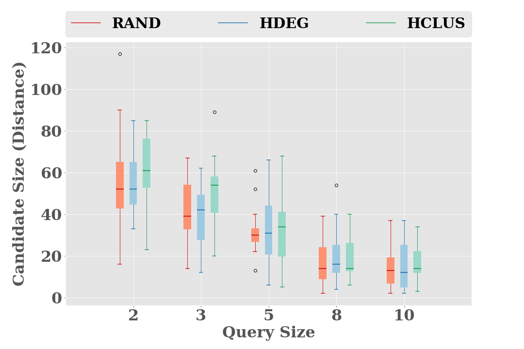
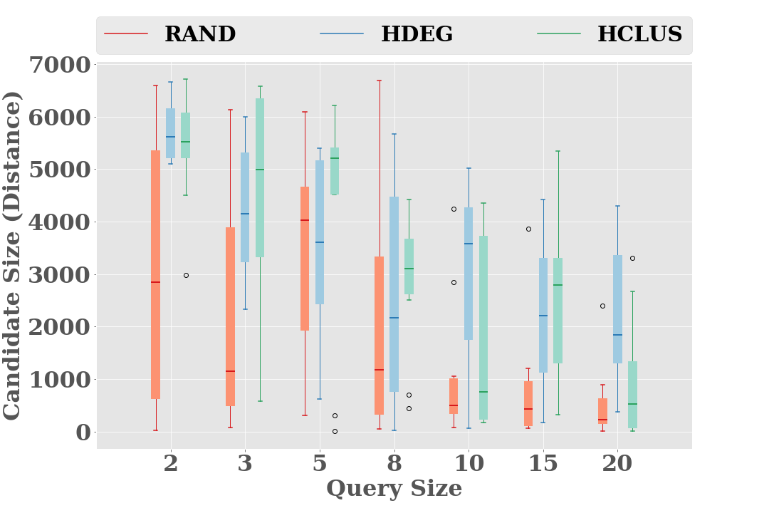
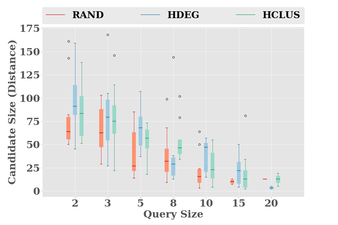
(a) Minnasota Road Network	(b) P2P Network	(c) USA Road Network

Figure 2. Box plot for the candidate skyline size with respect to the query size for the Minnasota Road Network, P2P Network, and USA Road Network datasets.

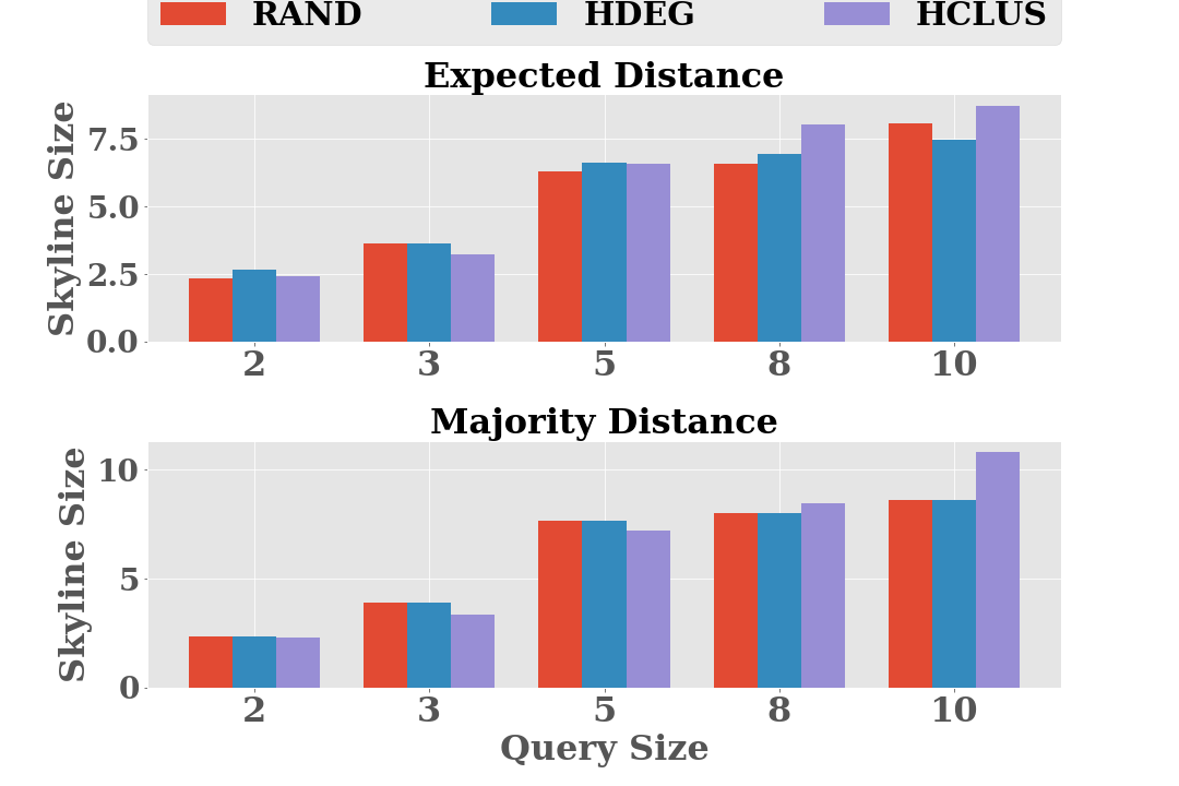
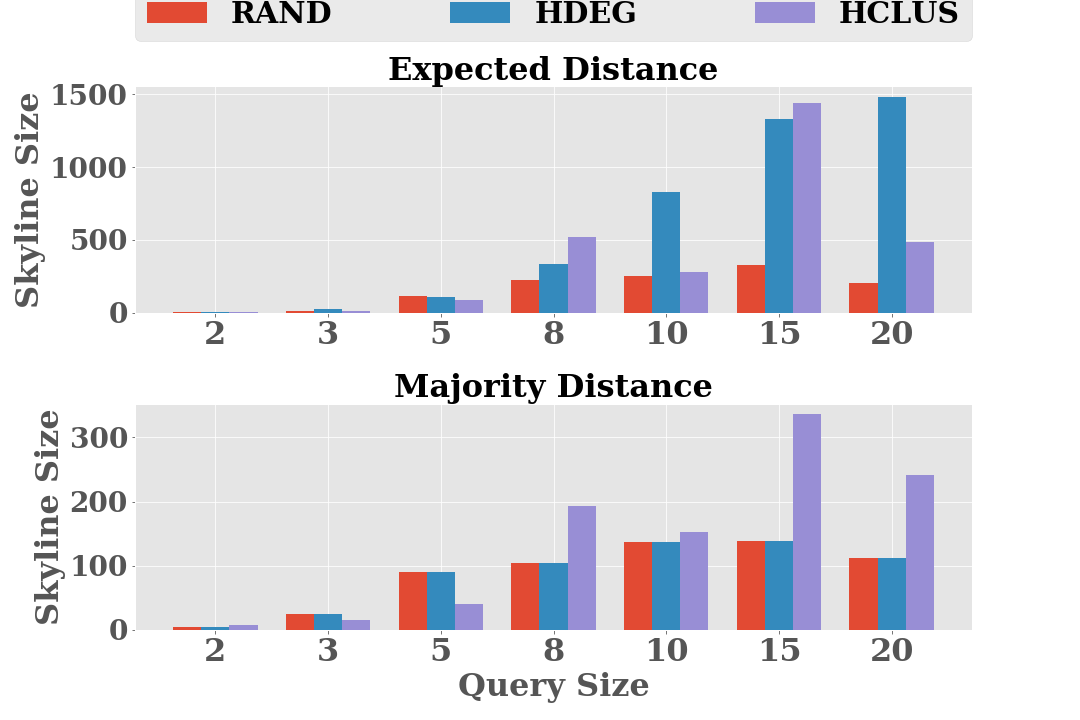
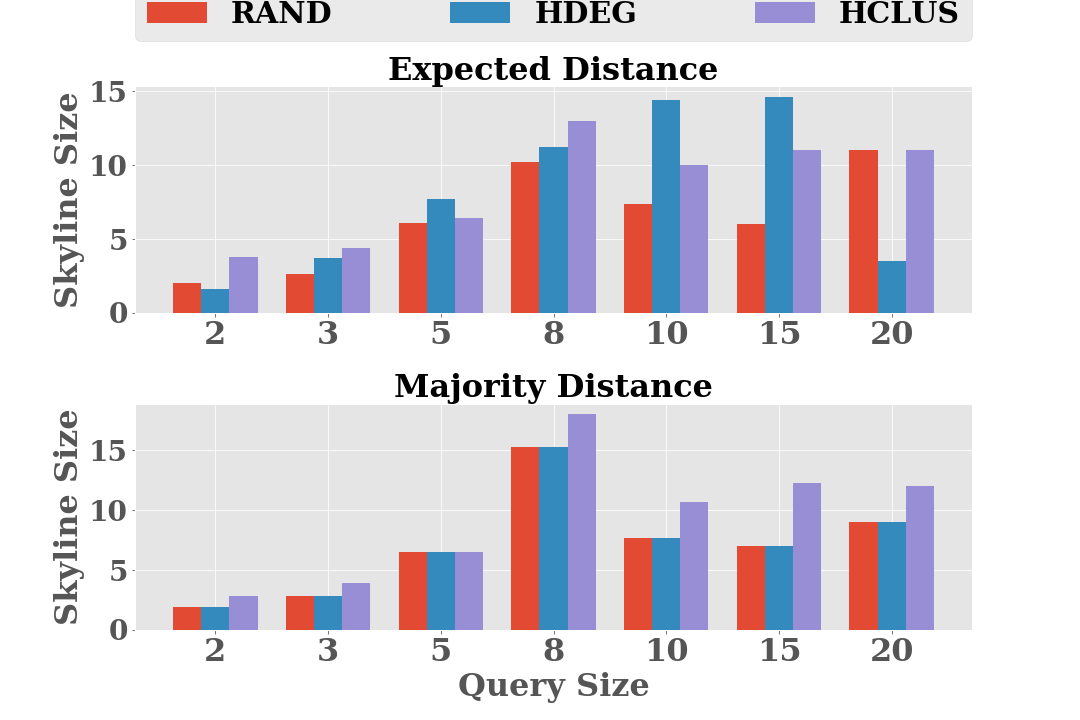
(a) Minnasota Road Network	(b) P2P Network	(c) USA Road Network

Figure 3. Query size Vs. Skyline size plot for the Minnasota Road Network, P2P Network, and USA Road Network datasets.

In this section we describe the experimental validations of our proposed approach. Initially, we start by describing the datasets.

4.1. Datasets

In our study, we have used three different datasets appeared in three different contexts described below.

• Minnesota Road Network (MRN) (Rossi and Ahmed, 2015): This is a road network dataset of the Minnasota city. Here, the junctions are represented by the nodes, and if two junctions are connected by a road then the corresponding two vertices are connected by an edge.

• P2P Network (Leskovec et al., 2007; Ripeanu and Foster, 2002):This dataset contains a sequence of snapshots of the Gnutella peer-to-peer file sharing network from August 2002. There are total of 9 snapshots of Gnutella network collected in August 2002. Nodes represent hosts in the Gnutella network topology and edges represent connections between the Gnutella hosts.

• USA Road Network (URN) (Rossi and Ahmed, 2015): This dataset describes a road network from the United States. Here, vertices represent the junctions, and an edge between signifies that the corresponding two junctions are are connected by road.

Please refer to Table 1 for basic statistics of the datasets. All the datasets are undirected and unweighted. Probability of existence and weight of each edge is chosen from the intervals $(0,1]$ and $[10,100]$ uniformly at random.

Table 1. Basic Statistics of the Datasets

Dataset	n	m	Density	Avg. Degree
MRN	2642	3300	$9.46\times 10^{-4}$	2
P2P Network	8114	26013	$7.90\times 10^{-4}$	6.41
URN	129164	165435	$1.98\times 10^{-5}$	2.56

4.2. Experimental Setup

In our study the following three different query vertex selection strategies have been adopted:

• RAND: By this method, to select $k$ query vertices first one is chosen randomly and remaining $(k-1)$ query vertices are chosen from the two hop neighbors of the initially selected vertex uniformly at random.

• HDEG: By this method, to select $k$ query vertices first the subset of the nodes whose degree is more than a threshold value are marked and a node is chosen uniformly at random as a query vertex. Remaining $(k-1)$ are chosen from the two hop neighbors of the initially selected vertices uniformly at random.

• HCLUS: This method is exactly the same as HDEG, except the case that, for choosing the first query vertex the subset of vertices are chosen based on the clustering coefficient of nodes.

Based on the selection strategy, we choose the query size from the set $\{2,3,5,8,10,15,20\}$. The experiments are repeated for 10 times. All the algorithms have been implemented with Python 3.5 + NetworkX 2.1 environment on a HPC Cluster with 5 nodes each of them having 64 cores and 160 GB of memory and the implementations are available at https://github.com/BITHIKA1992/Skyline_Uncertain_Graph/

4.3. Goals of the Experiments

The experiments that have been conducted here aim to address the following questions:

• Efficiency of the Pruning Strategies: As the number of query vertices increases, what is the fraction of data vertices removed before distance computation?

• Query Size Vs. Skyline Vertices: Under different query vertex selection strategies how the cardinality of the skyline vertex set changes with respect to the query size?

• Distance Metric Vs. Skyline Vertices: For a fixed query selection strategy and query size, how the cardinality of the skyline vertices changes with respect to the distance metric?

• Query Selection Strategy Vs. Skyline Vertices: For a fixed query size and distance metric how the cardinality of the skyline vertices changes with respect to query selection strategy?

• Query Size Vs. Computational Time: For a fixed query size and distance metric, how computational time grows with respect to query size?

4.4. Results and Discussion

Here, we address the research questions that we have raised.

4.4.1. Efficiency of the Pruning Strategies

As we apply BFS pruning in each dataset, it returns the vertices from the largest component. This reduces $3000$, and $114$ number of vertices for URN and P2P network dataset. For distance based pruning, we have taken the threshold value as $400$, considering 4-hop path with the maximum edge weight $100$. In Figure 2, we show the box plot for the candidate size with respect to each query size and the query selection strategy. It can be observed that the candidate size for RAND selection strategy is less than other two, in all the datasets, which is trivial to convince. For P2P network, the inter quartile range is very high compared to other datasets. This is due to the reason of high average degree in the network. Also, for RAND selection strategy, this range is the highest for small query size. This is due to the existence of various small size component in the network. Both the road networks are very sparse and for the large query sizes like 15, 20, the candidate size becomes very small and the variance also reduces. With this sparsity for small road network MRN, it is impossible to find the connected vertices from all the query vertices within the distance of 400. So, we remove the results for query size of 15 and 20 in MRN dataset.

Table 2. Computational time requirement (in Secs.) for finding skyline vertex set generation for Minnesota Road Network (MRN), P2P Network, and USA Road Network (URN) Dataset

Dataset	Query Size	Step 1			Step 2		Step 3	Total Time
		Sample Gen	B.F.S Pruning	Distance Pruning	MD Comp. Time	ED Comp. Time	Skyline Comp. Time	MD	ED
MRN	2	28.6028	0.0028	0.5797	0.2195	0.0328	0.0019	29.4070	0.6174
	3	29.3554	0.0029	0.6314	0.2232	0.0320	0.0021	30.2152	0.6685
	5	28.9936	0.0026	0.6565	0.2544	0.0365	0.0025	29.9098	0.6982
	8	30.3126	0.0029	0.7480	0.2443	0.0382	0.0029	31.3109	0.7922
	10	29.3217	0.0029	0.8090	0.3156	0.0487	0.0036	30.4530	0.8643
P2P Network	2	1585.5587	0.0135	494.5580	16676.0924	156.4454	0.0026	18756.2254	651.0197
	3	1596.0541	0.0142	737.8904	21824.5948	211.6984	0.0030	24158.5568	949.6062
	5	1594.3928	0.0149	1122.0655	27233.3476	299.2759	0.0159	29949.8369	1421.3723
	8	1583.5686	0.0148	1256.8362	26993.8274	406.0604	0.3052	29834.5524	1663.2167
	10	1619.4677	0.0140	1654.2035	39048.2783	572.3251	2.3940	42324.3577	2228.9368
	15	1567.8540	0.0153	2003.2736	44549.2078	707.3537	38.9008	48159.2516	2749.5436
	20	1611.6262	0.0168	2826.1580	60793.5038	954.3398	661.4532	65892.7582	4441.9679
URN	2	137954.2686	0.1908	52.9266	0.7025	0.0650	0.0039	138008.0926	53.1864
	3	139426.9728	0.1735	48.0920	0.7844	0.0730	0.0041	139476.0271	48.3427
	5	138948.9628	0.1743	54.1615	1.3545	0.1053	0.0063	139004.6596	54.4476
	8	163983.4069	0.1838	51.6949	1.2328	0.0928	0.0043	164036.5230	51.9759
	10	162627.5420	0.1947	57.9749	1.4499	0.1180	0.0070	162687.1688	58.2948
	15	115441.9538	0.1738	67.8932	0.8683	0.0847	0.0167	115510.9059	68.1685
	20	114801.2682	0.1805	79.6447	0.1371	0.0241	0.0107	114881.2415	79.8602

4.4.2. Query Size Vs. Skyline Vertices

In Figure 3, we show the plot for query size Vs. skyline size, with two distance metrics and three query selection strategies. In this part, we describe the comparison of sizes. From all the 10 executions, here we report the mean values for the skyline size. With the increase in query size, the skyline size increases. However, for URN dataset in Figure 3(c), the skyline size decreases for large value of query size. The reason is due to small size of candidate skyline, which can be verified from the Figure 2(c). Also, for both the road network datasets the maximum skyline size reaches to approximately 15, whereas for the P2P network it reaches to around 1500. This due to its candidate size. For, both the cases, at large value of query size the ratio of candidate to skyline size is very small. As the number of query vertices increase, the chance of domination decreases.

4.4.3. Distance Metric Vs. Skyline Vertices

In this part, referring to Figure 3, we describe the behavior of skyline size with respect to different distance metrics. For the road networks in Figure 3(a) and (c), the skyline size is similar in both the datasets. However, for the P2P network in Figure 3(b), the skyline size in the expected distance ($\approx$ max 1500) is much more than the majority distance ($\approx$ max 300). The reason lies on the networks high average degree value and the density. As the number of paths increases between a query vertex to a data vertex, the expected distance value is unable to dominate other data vertices. This results into large size of skyline vertex set. This can be verified from Figure 3(b), by looking into HDEG and and HCLUS selection strategies, where it differs from the expected distance results. However, for RAND, the size is similar in both the distances. From the experiments, we also observe that for a particular query vertex set the skyline vertices may not be the same from both the distance metrics.

4.4.4. Query Selection Strategy Vs. Skyline Vertices

In this part, referring to Figure 3, we describe the behavior of skyline size with respect to different query selection strategies. First, we describe the threshold value selected for HDEG and HCLUS for different datasets. As the P2P network dataset consists of high degree nodes, we select the high degree threshold value as 15, and it returns 440 nodes. In case of both the road networks, the maximum degree is around 5. Hence, for MRN and URN datasets, this threshold value is considered as 2 and 3, respectively. The clustering coefficient threshold is taken as 0 as the clustering coefficient for all the networks are very less. From Figure 3, the main observation is that for all the selection strategies the skyline size does not vary much for smaller query size. Whereas, for the large value of query size, HCLUS gives maximum skyline vertices.

4.4.5. Computational Time

Table 2 contains the stepwise computational time requirement to find skyline vertices for different datasets. From the table, it can be observed that for all the datasets as the query size increases, time requirement for finding out the skyline vertex set also increases. Due to the change in the query size, required time for distance-based pruning, distance and skyline computation (using BNL) increases. Also, for all the datasets, the main time requirement is due to the sample graph generation. As in case of expected distance sample generation is not required, hence, in this distance setting time requirement is much less compared to the majority distance. In particular, for query size $2$, the ratio between the computational time requirement for majority distance to expected distance for MRN, P2P, and URN are $47$, $28$, and $2556$, respectively.

Now, we proceed for the dataset specific observations. For the P2P Network dataset, when the query size increases beyond $10$, there is a sharp increase in the skyline computation time. This is due to the following two reasons. From the Figure 2(b) and 3(b), it can be observed that candidate and skyline size are more compared to the previous query sizes.

5. Conclusion and Future Directions

In this paper, we introduce the problem of dynamic skyline queries on uncertain graphs for two different distance measures, namely, majority distance and expected distance. For this problem, we have proposed a methodology having three main steps: pruning, distance computation, and skyline vertex set generation. The proposed methodology has been analyzed to understand its time and space requirement. The experimental results demonstrate that it can find out the skyline vertex set with reasonable computation time, particularly for the expected distance.

Now, this study can be extended in several directions. It will be an interesting future study to come up with efficient methodology, which can reduce the computational time even for majority distance. One possible way could be parallelizing the sample graph generation. It will be an important future work to provide a sample bound for the majority distance case. The minimum number of samples from the possible world, one should choose to answer the skyline with more than certain threshold probability.

- (1)
- Atallah and Qi (2009) Mikhail J Atallah and Yinian Qi. 2009. Computing all skyline probabilities for uncertain data. In Proceedings of the twenty-eighth ACM SIGMOD-SIGACT-SIGART symposium on Principles of database systems. ACM, 279–287.
- Bonchi et al. (2014) Francesco Bonchi, Francesco Gullo, Andreas Kaltenbrunner, and Yana Volkovich. 2014. Core decomposition of uncertain graphs. In Proceedings of the 20th ACM SIGKDD international conference on Knowledge discovery and data mining. ACM, 1316–1325.
- Borzsony et al. (2001) Stephan Borzsony, Donald Kossmann, and Konrad Stocker. 2001. The skyline operator. In Proceedings 17th international conference on data engineering. IEEE, 421–430.
- Chen et al. (2015) Yifan Chen, Xiang Zhao, Xuemin Lin, and Yang Wang. 2015. Towards frequent subgraph mining on single large uncertain graphs. In 2015 IEEE International Conference on Data Mining. IEEE, 41–50.
- Chen et al. (2018) Yifan Chen, Xiang Zhao, Xuemin Lin, Yang Wang, and Deke Guo. 2018. Efficient Mining of Frequent Patterns on Uncertain Graphs. IEEE Transactions on Knowledge and Data Engineering 31, 2 (2018), 287–300.
- Chomicki et al. (2013) Jan Chomicki, Paolo Ciaccia, and Niccolo’ Meneghetti. 2013. Skyline queries, front and back. ACM SIGMOD Record 42, 3 (2013), 6–18.
- De Matteis et al. (2015) Tiziano De Matteis, Salvatore Di Girolamo, and Gabriele Mencagli. 2015. A multicore parallelization of continuous skyline queries on data streams. In European Conference on Parallel Processing. Springer, 402–413.
- De Matteis et al. (2016) Tiziano De Matteis, Salvatore Di Girolamo, and Gabriele Mencagli. 2016. Continuous skyline queries on multicore architectures. Concurrency and Computation: Practice and Experience 28, 12 (2016), 3503–3522.
- Fu et al. (2017) Xiaoyi Fu, Xiaoye Miao, Jianliang Xu, and Yunjun Gao. 2017. Continuous range-based skyline queries in road networks. World Wide Web 20, 6 (2017), 1443–1467.
- Halim et al. (2017) Zahid Halim, Muhammad Waqas, Abdul Rauf Baig, and Ahmar Rashid. 2017. Efficient clustering of large uncertain graphs using neighborhood information. International Journal of Approximate Reasoning 90 (2017), 274–291.
- He et al. (2016) Guoliang He, Lu Chen, Chen Zeng, Qiaoxian Zheng, and Guofu Zhou. 2016. Probabilistic skyline queries on uncertain time series. Neurocomputing 191 (2016), 224–237.
- Hu et al. (2017) Jiafeng Hu, Reynold Cheng, Zhipeng Huang, Yixang Fang, and Siqiang Luo. 2017. On embedding uncertain graphs. In Proceedings of the 2017 ACM on Conference on Information and Knowledge Management. ACM, 157–166.
- Huang et al. (2018) Zhenhua Huang, Weicheng Xu, Jiujun Cheng, and Juan Ni. 2018. An efficient algorithm for skyline queries in cloud computing environments. China Communications 15, 10 (2018), 182–193.
- Jaudoin et al. (2017) Hélène Jaudoin, Pierre Nerzic, Olivier Pivert, and Daniel Rocacher. 2017. On Making Skyline Queries Resistant to Outliers. In Advances in Knowledge Discovery and Management. Springer, 19–38.
- Jiang and Du (2018) Bo Jiang and Xinjun Du. 2018. Personalized travel route recommendation with skyline query. In 2018 IEEE 9th International Conference on Dependable Systems, Services and Technologies (DESSERT). IEEE, 549–554.
- Jiang et al. (2016) Shunqing Jiang, Jiping Zheng, Jialiang Chen, and Wei Yu. 2016. K-th order skyline queries in bicriteria networks. In Asia-Pacific Web Conference. Springer, 488–491.
- Jin et al. (2011) Ruoming Jin, Lin Liu, and Charu C Aggarwal. 2011. Discovering highly reliable subgraphs in uncertain graphs. In Proceedings of the 17th ACM SIGKDD international conference on Knowledge discovery and data mining. ACM, 992–1000.
- Kassiano et al. (2016) Vasileios Kassiano, Anastasios Gounaris, Apostolos N Papadopoulos, and Kostas Tsichlas. 2016. Mining uncertain graphs: An overview. In International Workshop of Algorithmic Aspects of Cloud Computing. Springer, 87–116.
- Ke et al. (2019b) Xiangyu Ke, Arijit Khan, Mohammad Al Hasan, and Rojin Rezvansangsari. 2019b. Budgeted Reliability Maximization in Uncertain Graphs. arXiv preprint arXiv:1903.08587 (2019).
- Ke et al. (2019a) Xiangyu Ke, Arijit Khan, and Leroy Lim Hong Quan. 2019a. An in-depth comparison of st reliability algorithms over uncertain graphs. Proceedings of the VLDB Endowment 12, 8 (2019), 864–876.
- Keles and Hose (2019) Ilkcan Keles and Katja Hose. 2019. Skyline Queries over Knowledge Graphs. In The 18th International Semantic Web Conference, ISWC 2019International Semantic Web Conference. Springer.
- Khan and Chen (2015) Arijit Khan and Lei Chen. 2015. On uncertain graphs modeling and queries. Proceedings of the VLDB Endowment 8, 12 (2015), 2042–2043.
- Khan et al. (2012) Arijit Khan, Vishwakarma Singh, and Jian Wu. 2012. Finding Skyline Nodes in Large Networks. In 2012 IEEE 28th International Conference on Data Engineering Workshops. IEEE, 198–204.
- Khan et al. (2018) Arijit Khan, Yuan Ye, and Lei Chen. 2018. On Uncertain Graphs. Synthesis Lectures on Data Management 10, 1 (2018), 1–94.
- Le et al. (2016) Trieu Minh Nhut Le, Jinli Cao, and Zhen He. 2016. Answering skyline queries on probabilistic data using the dominance of probabilistic skyline tuples. Information Sciences 340 (2016), 58–85.
- Lee et al. (2016) Jongwuk Lee, Hyeonseung Im, and Gae-won You. 2016. Optimizing skyline queries over incomplete data. Information Sciences 361 (2016), 14–28.
- Leskovec et al. (2007) Jure Leskovec, Jon Kleinberg, and Christos Faloutsos. 2007. Graph evolution: Densification and shrinking diameters. ACM Transactions on Knowledge Discovery from Data (TKDD) 1, 1 (2007), 2.
- Liu et al. (2019) Jun Liu, Xiaoyong Li, Kaijun Ren, and Junqiang Song. 2019. Parallelizing uncertain skyline computation against n-of-N data streaming model. Concurrency and Computation: Practice and Experience 31, 4 (2019), e4848.
- Liu et al. (2018a) Jun Liu, Xiaoyong Li, Kaijun Ren, Junqiang Song, and Zongshuo Zhang. 2018a. Parallel n-of-N Skyline Queries over Uncertain Data Streams. In International Conference on Database and Expert Systems Applications. Springer, 176–184.
- Liu et al. (2018b) Jinfei Liu, Juncheng Yang, Li Xiong, and Jian Pei. 2018b. Secure and Efficient Skyline Queries on Encrypted Data. IEEE Transactions on Knowledge and Data Engineering 31, 7 (2018), 1397–1411.
- Miao et al. (2016) Xiaoye Miao, Yunjun Gao, Gang Chen, and Tianyi Zhang. 2016. k-dominant skyline queries on incomplete data. Information Sciences 367 (2016), 990–1011.
- Miao et al. (2018) Xiaoye Miao, Yunjun Gao, Su Guo, and Gang Chen. 2018. On efficiently answering why-not range-based skyline queries in road networks. IEEE Transactions on Knowledge and Data Engineering 30, 9 (2018), 1697–1711.
- Nguyen and Cao (2015) Ha Thanh Huynh Nguyen and Jinli Cao. 2015. Preference-based top-k representative skyline queries on uncertain databases. In Pacific-Asia Conference on Knowledge Discovery and Data Mining. Springer, 280–292.
- Ouyang et al. (2018) Dian Ouyang, Long Yuan, Fan Zhang, Lu Qin, and Xuemin Lin. 2018. Towards Efficient Path Skyline Computation in Bicriteria Networks. In International Conference on Database Systems for Advanced Applications. Springer, 239–254.
- Park et al. (2015) Yoonjae Park, Jun-Ki Min, and Kyuseok Shim. 2015. Processing of probabilistic skyline queries using MapReduce. Proceedings of the VLDB Endowment 8, 12 (2015), 1406–1417.
- Park et al. (2017) Yoonjae Park, Jun-Ki Min, and Kyuseok Shim. 2017. Efficient processing of skyline queries using MapReduce. IEEE Transactions on Knowledge and Data Engineering 29, 5 (2017), 1031–1044.
- Potamias et al. (2009) Michalis Potamias, Francesco Bonchi, Aristides Gionis, and George Kollios. 2009. Nearest-neighbor queries in probabilistic graphs. Technical Report. Boston University Computer Science Department.
- Ripeanu and Foster (2002) Matei Ripeanu and Ian Foster. 2002. Mapping the gnutella network: Macroscopic properties of large-scale peer-to-peer systems. In international workshop on peer-to-peer systems. Springer, 85–93.
- Rossi and Ahmed (2015) Ryan A. Rossi and Nesreen K. Ahmed. 2015. The Network Data Repository with Interactive Graph Analytics and Visualization. In AAAI. http://networkrepository.com
- Son et al. (2017) Wanbin Son, Fabian Stehn, Christian Knauer, and Hee-Kap Ahn. 2017. Top-k manhattan spatial skyline queries. Inform. Process. Lett. 123 (2017), 27–35.
- Wang et al. (2016) Yan Wang, Baoyan Song, Junlu Wang, Li Zhang, and Ling Wang. 2016. Geometry-based distributed spatial skyline queries in wireless sensor networks. Sensors 16, 4 (2016), 454.
- Yawalkar and Ranu (2019) Pranali Yawalkar and Sayan Ranu. 2019. Route Recommendations on Road Networks for Arbitrary User Preference Functions. In 2019 IEEE 35th International Conference on Data Engineering (ICDE). IEEE, 602–613.
- Yin et al. (2018) Bo Yin, Ke Gu, Xuetao Wei, Siwang Zhou, and Yonghe Liu. 2018. A cost-efficient framework for finding prospective customers based on reverse skyline queries. Knowledge-Based Systems 152 (2018), 117–135.
- Zeng et al. (2019) Yifu Zeng, Guo Chen, Kenli Li, Yantao Zhou, Xu Zhou, and Keqin Li. 2019. M-Skyline: Taking sunk cost and alternative recommendation in consideration for skyline query on uncertain data. Knowledge-Based Systems 163 (2019), 204–213.
- Zhang et al. (2019) Kaiqi Zhang, Hong Gao, Xixian Han, Zhipeng Cai, and Jianzhong Li. 2019. Modeling and Computing Probabilistic Skyline on Incomplete Data. IEEE Transactions on Knowledge and Data Engineering (2019).
- Zheng et al. (2014) Weiguo Zheng, Lei Zou, Xiang Lian, Liang Hong, and Dongyan Zhao. 2014. Efficient subgraph skyline search over large graphs. In Proceedings of the 23rd ACM International Conference on Conference on Information and Knowledge Management. ACM, 1529–1538.
- Zhou et al. (2016) Xu Zhou, Kenli Li, Guoqing Xiao, Yantao Zhou, and Keqin Li. 2016. Top favorite probabilistic products queries. IEEE Transactions on Knowledge and Data Engineering 28, 10 (2016), 2808–2821.
- Zhou et al. (2015) Xu Zhou, Kenli Li, Yantao Zhou, and Keqin Li. 2015. Adaptive processing for distributed skyline queries over uncertain data. IEEE Transactions on Knowledge and Data Engineering 28, 2 (2015), 371–384.
- Zhu et al. (2018) Xiaoyu Zhu, Jie Wu, Wei Chang, Guojun Wang, and Qin Liu. 2018. Authentication of Skyline Query over Road Networks. In International Conference on Security, Privacy and Anonymity in Computation, Communication and Storage. Springer, 72–83.
- Zou et al. (2010) Lei Zou, Lei Chen, M Tamer Özsu, and Dongyan Zhao. 2010. Dynamic skyline queries in large graphs. In International Conference on Database Systems for Advanced Applications. Springer, 62–78.