Interpreting Models of Infectious Diseases in Terms of Integral Input-to-State Stability

Abstract

This paper amis to develop a system-theoretic approach to ordinary differential equations which deterministically describe dynamics of prevalence of epidemics. The equations are treated as interconnections in which component systems are connected by signals. The notions of integral input-to-state stability (iISS) and input-to-state stability (ISS) have been effective in addressing nonlinearities globally without domain restrictions in analysis and design of control systems. They provide useful tools of module-based methods integrating characteristics of component systems. This paper expresses fundamental properties of models of infectious diseases and vaccination through the language of iISS and ISS. The systematic treatment is expected to facilitate development of effective schemes of controlling the disease spread via non-conventional Lyapunov functions.

1 Introduction

For many decades, mathematical models of infectious diseases have been recognized as useful tools for public health decision-making during epidemics KermackEpidemics27 ; ANDMAYnature79 ; HETHinfdiseas ; Keelinfdiseasbook09 . Detailed models help predict the future course of outbreak, while simple models allow one to understand mechanisms whose interpretations can lead to ideas of control strategies, such as vaccination, isolation, regulation and digital contact tracing or culling, which slow or ultimately eradicate the infection from the population. The objective of this paper is to facilitate the development of the latter. This paper does not report any novel behavior of disease transmission. Instead, this paper is devoted to a system and signal interpretation of behavior of classical and simple models of infectious diseases in the language of integral input-to-state stability (iISS) and input-to-state stability (ISS). It aims to take a first step toward development of an iISS/ISS-theoretic foundation for control design to combat infectious diseases. This paper reports that popular models share essentially the same qualitative behavior which can be analyzed and explained systematically via the same tools of iISS/ISS.

The notion of iISS and ISS have been accepted widely as mathematical tools to deal with and utilize nonlinearities effectively in the area of control SontagISS08 ; SONCOP ; SontagSCL98 . The notions offer a systematic framework of module-based design of control systems. Once a system or a network is divided into ‘stable” components, aggregating characteristics of components gives answers to control design problems systematically. The answers are global, and they are not restricted to small domains of variables. Without relying linearity, ISS allows one to handle systems based on boundedness of states with respect to bounded inputs. Importantly, the boundedness does not require finite operator gain, so that replacing linearity with ISS, we can handle a large class of nonlinear systems. However, nonlinearity such as bilinearity and saturation often prevent systems from being ISS. They are cases where nonlinearities retain convergence of state variables in the absence of inputs, but prevent state variables from being bounded in the presence of inputs. Such nonlinear systems are covered by iISS. Systems whose state is bounded for small inputs are grouped into the class of Strong iISS systems CHAANGITOStrISS14 . ISS and (Strong) iISS characterize both internal and external stability properties. The weak “stability” of (Strong) iISS components can be compensated by ISS components. This fact is one of useful and powerful tools of the iISS/ISS framework. Some of main ideas of iISS/ISS module-based arguments are packed in the iISS small-gain theorem ITOTAC06 ; ITOJIATAC09 ; ITOacc11neti ; ANGSGiISS which is an extension of the ISS small-gain theorem JIA96LYA ; KARJIAvectorSG09 ; LIUHILJIAcdc09 ; DRWsicon10 ; DASITOWIRejc11 . One of the important features of the small-gain methodology is that for interconnected systems and networks, it gives formula to explicitly construct non-conventional Lyapunov functions which not only establish stability properties of equilibria, but also properties with respect to external variables and parameters. For understanding behavior of diseases transmission, construction of Lyapunov functions has been one of major directions in mathematical epidemiology, and Lyapunov functions are known to be useful for analyzing global properties of stability of each given equilibrium (see KOROLyap02 ; KOROLyap04 ; FALLIDlypu07 ; OREGAN2010446 ; EnaNakIDlyapdelay11 ; NakEnaIDlyap14 ; SHUAIIDlyapu13 ; ChenLyapDI14 and references therein). However, the Lyapunov functions are classical, so that they do not unite characterizations of stability properties which vary with parameters and external elements. In other words, bifurcation analysis need to be performed separately to divide the Lyapunov function analysis into cases. In addition, it has been also common to make simplifying assumptions of precise population conservation that refuses external signals and perturbation of parameters (see, e.g., KOROLyap02 ; KOROLyap04 ; KOROgennonID06 ; OREGAN2010446 ; LIMULDseirlyapu95 ; EnaNakIDlyapdelay11 ).

This paper gives interpretations to behavior of typical models of infectious diseases in terms of basic characterizations of iISS and ISS SONISSV ; SontagSCL98 ; ANGSONiISS with the help of two tools provided by iISS and ISS. One tool is a criterion of the small-gain type. The other is a fusion of global and local nonlinear gain of components. The two tools formulated in this paper are not completely novel ideas, but they extend standard concepts in the iISS/ISS methodology by specializing in the setup of diseases models. In addition to their usefulness, this paper illustrates how the same set of the basic characterizations and tools of iISS/ISS can be applied to popular models of infectious diseases uniformly to help explain and capture their fundamental behavior globally without dividing the analysis into cases a prior.

2 Preliminaries

Let the set of real numbers be denoted by $\mathbb{R}:=(-\infty,\infty)$. This paper uses the symbols $\mathbb{R}_{+}:=[0,\infty)$ and $\mathbb{R}_{+}^{n}:=[0,\infty)^{n}$. The convention $\infty\leq\infty$ is used for notational simplicity. A function $\eta:\mathbb{R}_{+}\to\mathbb{R}_{+}$ is said to be of class $\mathcal{P}$ and written as $\eta\in\mathcal{P}$ if $\eta$ is continuous and satisfies $\eta(0)=0$ and $\eta(s)>0$ for all $s\in\mathbb{R}_{+}\setminus\{0\}$. A class ${\mathcal{P}}$ function is said to be of class $\mathcal{K}$ if it is strictly increasing, A class ${\mathcal{K}}$ function is said to be of class ${\cal K}_{\infty}$ if it is unbounded. A continuous function $\beta:\mathbb{R}_{+}\times\mathbb{R}_{+}\to\mathbb{R}_{+}$ is said to be of class $\mathcal{KL}$ if, for each fixed $t\geq 0$, $\beta(\cdot,t)$ is of class $\mathcal{K}$ and, for each fixed $s>0$, $\beta(s,\cdot)$ is decreasing and $\lim_{t\to\infty}\beta(s,t)=0$. The zero function of appropriate dimension is denoted by $0$. Composition of $\eta_{1},\eta_{2}:\mathbb{R}_{+}\to\mathbb{R}_{+}$ is expressed as $\eta_{1}\circ\eta_{2}$. For a continuous function $\eta:\mathbb{R}_{+}\to\mathbb{R}_{+}$, the function $\eta^{\ominus}$: $\mathbb{R}_{+}\to\overline{\mathbb{R}}_{+}:=[0,\infty]$ is defined as $\eta^{\ominus}(s)=\sup\{\tau\in\mathbb{R}_{+}:s\geq\eta(\tau)\}$. By definition, for $\eta\in\mathcal{K}$, $\eta^{\ominus}(s)=\infty$ holds for all $s\geq\lim_{\tau\to\infty}\eta(\tau)$, and $\eta^{\ominus}(s)=\eta^{-1}(s)$ elsewhere. The set $\{1,2,3,\ldots,n\}$ is denoted by $\overline{n}$. For a set $U$, its cardinality is denoted by $|U|$. For $U\subset\overline{n}$ and $x\in\mathbb{R}^{n}$, the vector $x_{U}\in\mathbb{R}^{|U|}$ is the collection of $|U|$ components $x_{i}$, $i\in U$.

A system of the form

$$\dot{x}(t)=f(x(t),u(t))$$ (1)

is said to be integral input-to-state stable (iISS) with respect to the input $u$ SontagSCL98 if there exist $\beta\in\mathcal{KL}$, $\chi$, $\mu\in{\mathcal{K}}\cup\{0\}$ such that, for all measurable locally essentially bounded functions $u:\mathbb{R}_{+}\to\mathbb{R}^{p}$, all $x(0)\in\mathbb{R}^{n}$ and all $t\geq 0$, its solution $x(t)$ exists and satisfies

$$|x(t)|\leq\beta(|x(0)|,t)+\chi\left(\int_{0}^{t}\mu(|u(\tau)|)d\tau\right),$$ (2)

where the symbol $|\cdot|$ denotes the Euclidean norm. System (1) is said to be strongly integral input-to-state stable (Strongly iISS) with respect to the input $u$ CHAANGITOStrISS14 if there exist $R>0$ and $\gamma\in{\mathcal{K}}\cup\{0\}$ such that

$${\operatorname*{ess\,sup}}_{t\in\mathbb{R}_{+}}|u(t)|<R\ \Rightarrow\$$

$$\hskip 25.83325pt|x(t)|\leq\beta(|x(0)|,t)+\gamma({\operatorname*{ess\,sup}}_{t\in\mathbb{R}_{+}}|u(t)|)$$ (3)

holds in addition to the above requirement (2). The constant $R$ is called an input threshold. If the requirement (3) is met with $R=\infty$, system (1) is said to be input-to-state stable (ISS) SONCOP . The function $\gamma$ is called an ISS-gain function. An ISS system is Strongly iISS. A Strongly iISS system is iISS. Their converses do not hold true. iISS of (1) implies globally asymptotic stability of the equilibrium $x=0$ for $u=0$. If a radially unbounded and continuously differentiable function $V:\mathbb{R}^{n}\to\mathbb{R}_{+}$ satisfies

$$\forall x\in\mathbb{R}^{n}\hskip 6.45831pt\forall u\in\mathbb{R}^{p}\hskip 6.45831pt\frac{\partial V}{\partial x}(x)f(x,u)\leq-\alpha(V(x))+\sigma(|u|)$$ (4)

for some $\sigma\in\mathcal{K}$ and some $\alpha\in\mathcal{P}$ (resp., $\alpha\in\mathcal{K}$ and $\lim_{s\to\infty}\alpha(s)\geq\lim_{s\to\infty}\sigma(s)$), the function $V(x)$ is said to be an iISS (resp., ISS) Lyapunov function. The existence of an iISS (resp., ISS) Lyapunov function guarantees iISS (resp., ISS) of system (1) ANGSONiISS ; SONISSV . If an iISS Lyapunov function admits $\alpha\in\mathcal{K}$ in (4), the system is guaranteed to be Strong iISS CHAANGITOStrISS14 . iISS and ISS Lyapunov functions are conventional Lyapunov functions when the input $u$ is zero in system (1). The Lyapunov-type characterization (4) yields

$$\limsup_{t\to\infty}V(x(t))\leq\overline{\gamma}({\operatorname*{ess\,sup}}_{t\in\mathbb{R}_{+}}|u(t)|),$$ (5)

where $\overline{\gamma}:=\alpha^{\ominus}\circ\sigma$. If $u(t)\equiv u_{0}$ is a constant and (4) holds with an equality sign, we have $\lim_{t\to\infty}V(x(t))=\overline{\gamma}(|u_{0}|)$. The inequality (5) is called the asymptotic gain property SONISSV . If system (1) is not ISS, there exists no $\overline{\gamma}\in\mathcal{K}$ satisfying the asymptotic gain property (5). This is because (3) never holds with $R=\infty$. As in (2), an iISS system which is not ISS accumulates its input, and the solution $x(t)$ exists for all $t\in\mathbb{R}_{+}$, but unbounded if the input is persistent. All the above are standard definitions given for sign-indefinite system (1). When the vector field $f$ generates only non-negative $x(t)$ in (1) defined with $x(0)\in\mathbb{R}_{+}^{n}$ and $u(t)\in\mathbb{R}_{+}^{p}$, all the above definitions and facts are valid by replacing $\mathbb{R}$ with $\mathbb{R}_{+}$.

3 A Small-Gain Theorem for Generalized Balancing Kinetics

This section shows a small-gain type method for establishing stability of dynamical networks in the framework of iISS. To propose a generalized formulation which includes a previously-developed criterion as a special case, consider $x(t)=[x_{1}(t),x_{2}(t),\ldots,x_{n}(t)]^{T}:\mathbb{R}_{+}\to\mathbb{R}_{+}^{n}$ governed by

$$\dot{x}_{i}= -\eta_{i-1,i}(x)+\sigma_{i,i-1}(x)-\eta_{i+1,i}(x)$$

$$\hskip 8.61108pt+\sigma_{i,i+1}(x)-\theta_{i}(x_{i})+\kappa_{i}(w_{i}),\hskip 17.22217pti\in\overline{n}$$ (6)

for any $x(0)\in\mathbb{R}_{+}^{n}$ and any measurable and locally essentially bounded function $w(t)=[w_{1}(t),w_{2}(t),\ldots,w_{n}(t)]^{T}\in\mathbb{R}_{+}^{n}$. In (6), the subscripts of $\eta$ and $\sigma$ are integers which are circular of length $n$. If a subscript $k$ by itself does not belong to $\overline{n}$, it stands for $((k-1)\,\mathrm{mod}\,n)+1$, where $i\,\mathrm{mod}\,n$ denotes the non-negative reminder of the division of an integer $i$ by $n$. All subscripts in this section are circular. Assume that the functions $\eta_{i-1,i}$, $\eta_{i+1,i}$, $\sigma_{i,i-1}$, $\sigma_{i,i+1}:\mathbb{R}_{+}^{n}\to\mathbb{R}_{+}$ and $\theta_{i}\in\mathcal{P}$ are locally Lipschitz and satisfy

$$x_{i}=0\hskip 7.74998pt\Rightarrow\hskip 7.74998pt\eta_{i-1,i}(0)=\eta_{i+1,i}(0)=0$$ (7)

for all $i\in\overline{n}$. For all $i\in\overline{n}$, $\kappa_{i}\in\mathcal{K}\cup\{0\}$ is assumed. Network (6) is made of balancing mechanisms between state variables. The component $x_{i}$ is consumed at the rate $-\eta_{i+1,i}(x)$, and the consumption leads to the production of the downstream component $x_{i+1}$ at the rate $+\sigma_{i+1,i}(x)$. In the same way, the consumption $-\eta_{i-1,i}(x)$ of $x_{i}$ produces the upstream component $x_{i-1}$ at the rate $+\sigma_{i-1,i}(x)$. The rates are allowed to be functions of $x$ instead of the local variable $x_{i}$. The extra rate $\theta_{i}$ of consumption in either the upstream or the downstream direction is a function of the local variable $x_{i}$. It is also important that the balancing between neighbors forms not only cycles of length $1$, but also cycles of length $n$. Assume that the rate functions in (6) satisfy

$$\forall i\in\overline{n}\hskip 4.30554pt\forall j\in\{i-1,i+1\}\hskip 6.45831pt\exists\ell_{i,j}\geq 0\hskip 6.45831pt\forall x\in\mathbb{R}_{+}^{n}\hskip 6.45831pt\sigma_{i,j}(x)\leq\ell_{i,j}\eta_{i,j}(x).$$ (8)

The following theorem can be proved.

Theorem 1

Assume that

$$\forall i\in\overline{n}\hskip 6.45831pt\ell_{i,i+1}\ell_{i+1,i}\leq 1$$ (9)

$$\exists k\in\overline{n}\hskip 6.45831pt\ell_{k,k+1}\ell_{k+1,k}\leq\prod_{i=1}^{n}\dfrac{\ell_{i,i+1}}{\ell_{i+1,i}}\leq\frac{1}{\ell_{k,k+1}\ell_{k+1,k}}$$ (10)

are satisfied. Then network (6) is iISS with respect the input $w$. If $\theta_{i}\in\mathcal{K}$ (resp., $\theta_{i}\in\mathcal{K}_{\infty}$) holds for all $i\in\overline{n}$ in addition, network (6) is Strongly iISS (resp., ISS) with respect the input $w$. Furthermore, an iISS/ISS Lyapunov function $V(x)$ is

$$V(x)=\sum_{i\in\overline{n}}\lambda_{i}x_{i}$$ (11)

$$\forall i\!\in\!\{k\!+\!1,k\!+\!2,\ldots,k\!+\!n\}\hskip 6.45831pt\lambda_{i}=\!\!\prod_{j=k+2}^{i}\!\!\sqrt{\frac{\ell_{j-1,j}}{\ell_{j,j-1}}}.$$ (12)

Proof: Due to (9), from (8) and (12) it follows that

$$\lambda_{i+1}\sigma_{i+1,i}(x) =\sqrt{\dfrac{\ell_{i,i+1}}{\ell_{i+1,i}}}\lambda_{i}\sigma_{i+1,i}(x)$$

$$\leq\sqrt{\ell_{i,i+1}\ell_{i+1,i}}\lambda_{i}\eta_{i+1,i}(x_{i})\$$

$$\leq\lambda_{i}\eta_{i+1,i}(x)$$

$$\lambda_{i}\sigma_{i,i+1}(x) =\sqrt{\dfrac{\ell_{i+1,i}}{\ell_{i,i+1}}}\lambda_{i+1}\sigma_{i,i+1}(x)$$

$$\leq\lambda_{i+1}\eta_{i,i+1}(x)$$

for all $x\in\mathbb{R}_{+}^{n}$ at each $i\in\{k+1,k+2,\ldots,k+n-1\}$. By virtue of the second inequality in (10), properties (8) and (12) yield

$$\lambda_{k}\sigma_{k,k+1}(x) =\prod_{i=k+1}^{k+n-1}\sqrt{\dfrac{\ell_{i,i+1}}{\ell_{i+1,i}}}\lambda_{k+1}\sigma_{k,k+1}(x)$$

$$\leq\sqrt{\dfrac{\ell_{k+1,k}}{\ell_{k,k+1}}\cdot\frac{1}{\ell_{k,k+1}\ell_{k+1,k}}}\lambda_{k+1}\sigma_{k,k+1}(x)$$

$$\leq\lambda_{k+1}\eta_{k,k+1}(x).$$

In the same way, the first inequality in (10) gives

$$\lambda_{k+1}\sigma_{k+1,k}(x)\leq\lambda_{k}\eta_{k+1,k}(x).$$

Therefore, the function $V$ given in (11) satisfies

$$\dot{V}\leq\sum_{i\in\overline{n}}\lambda_{i}\left(-\theta_{i}(x_{i})+k_{i}(w_{i})\right)$$

along the trajectory $x(t)$ of network (6). Defining

$$\alpha(s):=\min_{\{x\in\mathbb{R}_{+}^{n}:V(x)=s\}}\sum_{i\in\overline{n}}\theta_{i}(x_{i})$$

$$\sigma(s):=\sum_{i\in\overline{n}}\kappa_{i}(s)$$

satisfies $\alpha\in\mathcal{P}$, $\kappa_{i}\in{\mathcal{K}}\cup\{0\}$ and (4). Therefore, the function $V$ is an iISS Lyapunov function establishing iISS of network (6). We have $\alpha\in\mathcal{K}$ establishing Strong iISS of network (6) if $\theta_{i}\in\mathcal{K}$ for all $i\in\overline{n}$. In the case of $\theta_{i}\in\mathcal{K}_{\infty}$ for all $i\in\overline{n}$, we have $\alpha\in\mathcal{K}_{\infty}$, and the function $V$ is an ISS Lyapunov function. $\square$

Recall that circulating subscripts of length $n$ are used for $\ell_{i,j}$ and $\lambda_{i}$. The above theorem extends a development of HITOconservcdc20 in which $\eta_{j,i}$ and $\sigma_{j,i}$ were restricted to be functions of $x_{i}$. The restriction disallows bilinearities and multiplicative nonlinearities to appear in $\eta_{j,i}$ and $\sigma_{j,i}$. Removal of the restrictions by Theorem 1 is the theoretical key in this paper.

Remark 1

If there exists $k\in\overline{n}$ such that $\ell_{k,k+1}=0$ achieving (8), the first inequality in (10) is satisfied automatically with a sufficiently small $\ell_{k+1,k}>0$. The same applies to the case of $\ell_{k,k+1}=0$ with the second inequality in (10).

Remark 2

Theorem 1 reduces to a special case of the iISS small-gain theorem for networks proposed in ITOacc11neti . When the functions in (6) are restricted to

$$\exists b_{i-i,i},b_{i+i,i}>0\hskip 6.45831pt\forall x\in\mathbb{R}_{+}^{n}\hskip 6.45831pt$$

$$\hskip 25.83325ptb_{i-i,i}\eta_{i-i,i}(x)=b_{i+i,i}\eta_{i+i,i}(x)=\theta_{i}(x_{i})$$ (13)

$$\theta_{i}\in\mathcal{K}$$ (14)

$$\forall x\in\mathbb{R}_{+}^{n}\hskip 6.45831pt\forall\hat{x}\in\mathbb{R}_{+}^{n}\cap\{\hat{x}_{i}=x_{i}\}\hskip 6.45831pt$$

$$\hskip 25.83325pt\sigma_{i,i-i}(x)\!=\!\sigma_{i,i-i}(\hat{x}),\ \sigma_{i,i+i}(x)\!=\!\sigma_{i,i+i}(\hat{x})$$ (15)

for all $i\in\overline{n}$, network (6) fit in the setup of ITOacc11neti , and the conditions (9) and (10) coincide with the cyclic small-gain condition presented in ITOacc11neti , If all the functions in (6) are non-zero, the network consists of $n$ simple directed cycles of length $1$, and $2$ simple directed cycles of length $n$. the inequality (9) is the small-gain requirement for the cycles of length $1$, while the two inequalities in (10) are for length $n$.

4 Convergence via Zero Local ISS-Gain

This section focuses on an extra property which iISS systems often possess due to bilinear or multiplicative nonlinearities. To formulate it, consider $x(t)\in\mathbb{R}_{+}$ governed by

$$\dot{x}=f(x,w):=\left[\begin{matrix}f_{1}(x,w)\\ f_{2}(x,w)\\ \vdots\\ f_{n}(x,w)\end{matrix}\right]$$ (16)

for any $x(0)\in\mathbb{R}_{+}^{n}$ and any measurable and locally essentially bounded function $w(t)=[w_{1}(t),w_{2}(t),\ldots,w_{p}(t)]^{T}\in\mathbb{R}_{+}^{p}$. It is assumed that $f:\mathbb{R}_{+}^{n}\times\mathbb{R}_{+}^{p}\to\mathbb{R}$ is locally Lipschitz functions satisfying $f(0,0)=0$ and

$$x_{i}=0\ \Rightarrow\ \forall x\in\mathbb{R}_{+}^{n}\hskip 6.45831pt\forall w\in\mathbb{R}_{+}^{p}\hskip 6.45831ptf_{i}(x,w)\geq 0.$$ (17)

Property (17) is necessary and sufficient for guaranteeing $x(t)\in\mathbb{R}_{+}^{n}$ with respect to all $x(0)$ and $w$. The following proposition describes a property of iISS systems which completely reject the effect of small inputs on some state variables.

Proposition 1

Suppose that system (16) is iISS with respect the input $w$, and admits a non-empty set $U\subset\overline{n}$, a radially unbounded and continuously differentiable function $V_{U}:\mathbb{R}^{|U|}\to\mathbb{R}_{+}$, and class $\mathcal{K}$ functions $\alpha_{U}$, $\sigma_{U}$ such hat

$$\forall x\in\mathbb{R}_{+}^{n}\hskip 6.45831pt\forall w\in\mathbb{R}_{+}^{p}\hskip 6.45831pt\hskip 6.45831pt\frac{\partial V_{U}}{\partial x_{U}}(x_{U})f_{U}(x,w)\leq-\alpha_{U}(V_{U}(x_{U}))+\sigma_{U}(w).$$ (18)

If there exist a non-empty set $L\subset\overline{n}$, a real number $H>0$, and a radially unbounded and continuously differentiable function $V_{L}:\mathbb{R}^{|L|}\to\mathbb{R}_{+}$ such that for each $k\in(0,1)$,

$$\forall x\in\mathbb{R}_{+}^{n}\cap\left\{V_{U}(x_{U})\leq kH\right\}\hskip 6.45831pt\forall w\in\mathbb{R}_{+}^{p}\hskip 6.45831pt\frac{\partial V_{L}}{\partial x_{L}}(x_{L})f_{L}(x,w)\leq-\alpha_{L}(V_{L}(x_{L}))$$ (19)

holds for some $\alpha_{L}\in\mathcal{P}$, then the solution $x(t)$ of (16) satisfies

$$\sup_{t\in\mathbb{R}_{+}}w(t)<Q\ \Rightarrow\ \forall x(0)\in\mathbb{R}_{+}^{n}\hskip 6.45831pt\lim_{t\to\infty}x_{L}(t)=0$$ (20)

for $Q=\lim_{s\to H-}\sigma_{U}^{\ominus}\circ\alpha_{U}(s)$.

Proof: Since system (16) is iISS, a solution $x(t)<\infty$ exists and unique for all $t\in\mathbb{R}_{+}$. Assume that a real number $H\in(0,\infty)$ satisfies (19). Suppose that $\sup_{t\in\mathbb{R}_{+}}w(t)<Q$ for $Q=\lim_{s\to H-}\sigma_{U}^{\ominus}\circ\alpha_{U}(s)$. In the case of $Q=\infty$, for each $w$, assumption (18) implies the existence of $T\in\mathbb{R}_{+}$ and $\epsilon\in(0,H)$ such that

$$\forall t\in[T,\infty)\hskip 6.45831ptV_{U}(x_{U}(t))\leq H-\epsilon.$$ (21)

In the case of $Q<\infty$, since for each $w$, there exists $\delta>0$ satisfying $\sup_{t\in\mathbb{R}_{+}}w(t)\leq Q-\delta$ , evaluating (18) allows one to verify the existence of $T\in\mathbb{R}_{+}$ and $\epsilon\in(0,H)$ fulfilling (21) again. Therefore, the existence of $\alpha_{L}\in\mathcal{P}$ satisfying (19) for each $k\in(0,1)$ ensures (20). $\square$

The above proposition makes use of property (19) which is the existence of a partial system completely rejecting the effect of its interconnecting inputs whose magnitude is smaller than a threshold. Let $L^{C}=\overline{n}\setminus L$. For $x_{L}$-system defined by $\dot{x}_{L}=f_{L}(x,w)$, $x_{L^{C}}(t)$ and $w(t)$ are exogenous. Property (19) implies that the ISS-gain from the input $[x_{L^{C}}^{T},w^{T}]^{T}$ to the state $x_{L}$ is zero as long as $V_{U}(x_{U})<H$. Hence, in Proposition 1, $x_{L}$-system is required to admit zero ISS-gain locally, although it is not required to be ISS globally. In the case of $L=\overline{n}$, property (19) implies Strong iISS of $x_{L}$-system since iISS is assumed in Proposition 1. This property (19) is very common, although it may not have been focused very often in the literature of systematic control methodology. For example, any of scalar non-negative systems

$$\dot{\xi}=-\xi+\xi w$$

$$\dot{\xi}=-\frac{\xi}{1+\xi}+\frac{\xi w}{1+\xi}$$

$$\dot{\xi}=-\frac{\xi}{1+\xi^{2}}+\frac{\xi w}{1+\xi^{2}}$$

has the threshold at $H=1$ for $x_{L}=\xi$ and $V(x_{L})=x_{L}$. The state $\xi$ converges to zero for $w<1$, while $\xi$ increases as long as $w>1$, although the increase is within the property of iISS . The above three systems are Strong iISS. The zero local ISS-gain they actually have is “stronger” than Strong iISS. In this way, the threshold is a bifurcation point bringing in a superior stability property. Bilinearity and multiplicative nonlinearity give rise to the bifurcation, and Proposition 1 aims at highlighting such systems.

Remark 3

Since Proposition 1 assumes the entire system (16) to be only iISS, the variable $x_{L}(t)$ can increase until $V_{U}(x_{U}(t))<H$ is achieved. Then an outbreak of $x_{L}$ occurs, and $x_{L}(t)$ exhibits a peak. Property (18) allows one to estimate that the smaller $w$ is, the shorter the time when $x_{L}$ starts decreasing (the duration of the growth phase) is. The larger $Q$ or $H$ is, the shorter the growth phase is. The increasing rate of $x_{L}(t)$ until $V_{U}(x_{U}(t))<H$ can be estimated by the iISS property of the entire system, or $x_{L}$-system, which is more specific than the entire system. For example, an upper bound of $({\partial V_{L}}/{\partial x_{L}})f_{L}$ for $V_{U}(x_{U})>H$ gives such information, which is not stated explicitly in Proposition 1.

5 SIR Model

Consider the solution $x(t):=[S(t),I(t),R(t)]^{T}\in\mathbb{R}_{+}^{3}$ of the ordinary differential equation

$$\dot{S}= B-\mu S-\beta IS$$ (22a)

$$\dot{I}= \beta IS-\gamma I-\mu I$$ (22b)

$$\dot{R}= \gamma I-\mu R$$ (22c)

defined for any $[S(0),I(0),R(0)]^{T}\in\mathbb{R}_{+}^{3}$ and any measurable and locally essentially bounded function $B:\mathbb{R}_{+}\to\mathbb{R}_{+}$ . The variable $S(t)$ describes the (continuum) number of susceptible population. $I(t)$ is the number of infected individuals, while $R(t)$ is of individuals recovered with immunity. $B(t)$ is the newborn/immigration rate. The positive number $\beta$, $\gamma$ and $\mu$ are parameters describing the contact rate, the recovery rate and the death rate, respectively. The equation (22) is referred to as the (classic) SIR endemic model HETHinfdiseas . When $B=0$ and $\mu=0$, the equation is referred to as the (classic) SIR epidemic model.

S-system (22a) and R-system (22c) are ISS with respect to the input $[B,I]^{T}$ and the input $I$, respectively. In fact, the positive variables $S$ and $R$ by themselves are ISS Lyapunov functions, due to the definition (4). The ISS property is also clear since R-system (22c) is linear, and S-system (22a) is bounded from above by the solution of the linear system $\dot{S}=B-\mu S$. The two linear systems are asymptotically stable. By contrast, due to the bilinear term $\beta IS$, I-system (22b) is not ISS with respect to the input $S$ since (22b) generates unbounded $I(t)$ for any constant input $S>(\gamma+\mu)/\beta$. I-system (22b) is Strong iISS since $V_{I}(I)=\log(1+I)$ yields

$$\dot{V}_{I}\leq-\frac{(\gamma+\mu)I}{1+I}+\beta S.$$

Hence, the SIR model (22) is a cascade consisting of an ISS system, an Strong iISS system and an ISS system. The argument of iISS cascade analysis CHAIANGmtns06 ; ITOTAC06 ; ITOTAC10 ; CHAANGITOStrISScas14 ; HITOcasSICE17 can show that the SIR model (22) is Strong iISS with respect to the input $B$. This stability assessment is not yet very informative, although it holds true. The rest this section demonstrates that the developments in Sections 3 and 4 improve the stability assessment for capturing discriminative behavior of the spread of infectious diseases.

Theorem 1 establishes that the SIR model (22) is ISS, which is “stronger” than Strong iISS, although the SIR model involves I-system which is not ISS. In fact, the model (22) satisfies (6) and (8) with

$$\ell_{i+1,i}=\ell_{i,i+1}=1,\ \theta_{i}(s)=\mu s,\ i=1,2,3.$$ (23)

These parameters satisfy (9) and (10), and yield $\lambda_{1}=\lambda_{2}=\lambda_{3}=1$. Theorem 1 gives the total number $N(t):=S(t)+I(t)+R(t)=V(x(t))$ as an ISS Lyapunov function for the SIR model (22). Indeed,

$$\dot{N}=-\mu N+B$$ (24)

is satisfied along the solution $x(t)$ of (22). The above inequality implies

$$\lim_{t\to\infty}N(t)=\frac{B}{\mu}$$ (25)

for any constant $B\in\mathbb{R}_{+}$. If $B$ is not constant, we have the asymptotic gain property

$$\limsup_{t\to\infty}N(t)\leq\frac{1}{\mu}\operatorname*{ess\,sup}_{t\in\mathbb{R}_{+}}B(t).$$ (26)

SI-system consisting of (22a) and (22b) is ISS with respect to the input $B$ since defining the sum $V_{U}(x_{U}(t))=S(t)+I(t)$ yields

$$\dot{V}_{U}=-\mu V_{U}-\gamma I+B$$

for $x_{U}=[S,I]^{T}$. This confirms (18) with $\alpha_{U}(s)=\mu s$ and $\sigma_{U}(s)=s$. I-system defined by (22b) fulfills (19) with $x_{L}=I$ and

$$H:=\frac{\gamma+\mu}{\beta}$$ (27)

since $S\leq V_{U}(x_{U})$. Recall that ISS of the entire model (22) implies iISS of (22). Hence, Proposition 1 with $Q=\mu H$ guarantees

$$\operatorname*{ess\,sup}_{t\in\mathbb{R}_{+}}{B}(t)<\mu H\ \Rightarrow\ \lim_{t\to\infty}I(t)=0.$$ (28)

The convergence of $I$ to zero implies $\lim_{t\to\infty}R(t)=0$ since (22c) is ISS. Indeed, it is a stable linear system. Thus

$$\operatorname*{ess\,sup}_{t\in\mathbb{R}_{+}}{B}(t)<\mu H\ \Rightarrow\ \lim_{t\to\infty}I(t)=\lim_{t\to\infty}R(t)=0.$$ (29)

For any constant $B\in\mathbb{R}_{+}$, by virtue of (25) or (22a), we arrive at

$${B}<\mu H\ \Rightarrow\ \lim_{t\to\infty}x(t)=\left[\frac{B}{\mu},0,0\right]^{T}.$$ (30)

As Proposition 1 is applied in the above analysis, regarding $S$ as a parameter, I-system has a bifurcation point at $S=H$. The origin $I=0$ is an unstable equilibrium if $S>H$. As explained in Remark 3, $I(t)$ increases until $S(t)\leq H$. It is not a possibility any more and the growth phase occurs since I-system is not ISS. In the case of ${B}<\mu H$ and $S(0)>H$, if $I(0)>0$, the infected population $I(t)$ peaks before converging to zero. The smaller $B$ and the larger $(\gamma+\mu)/\beta$ are, the shorter the time to the peak is. The larger $\mu$ and the smaller $\beta$ are, the smaller the increase rate of $I$ in the growth phase is.

Typical responses of the SIR model (22) are shown in Fig. 1 and Fig. 2 for $\beta=0.0002$, $\mu=0.015$ and $\gamma=0.032$ with $S(0)=700$, $I(0)=200$ and $R(0)=70$. For a general newborn/immigration rate $B$, the SIR model (22) is ISS. It means that the disease can remain as endemic. That is, the infected population $I(t)$ is bounded, but it can become very large, and $\liminf_{t\to\infty}I(t)>0$ can hold. Since $I$-system is Strong iISS and it is not ISS, the infected $I(t)$ starts with an growth phase unless the initial susceptible population is below the threshold $H=235$. The infected population $I(t)$ never decreases to zero if the newborn/immigration rate $B$ is above the threshold $\mu H=3.525$ (Fig. 1). If the newborn/immigration rate $B$ does not exceed the threshold, the convergence of $I(t)$ to zero is guaranteed, and the disease is eradicated (Fig. 2). This bifurcation is the central feature of the SIR model (22).

In mathematical epidemiology, for constant $B\in\mathbb{R}_{+}$, the value

$$R_{0}:=\frac{\beta B}{\mu(\gamma+\mu)}=\frac{B}{\mu H}$$ (31)

is called the basic reproduction number. Solving the simultaneous equation of $\dot{S}=0$, $\dot{I}=0$ and $\dot{R}=0$ in (22) with constant $B\in\mathbb{R}_{+}$ gives the steady-state value in (30) and

$$R_{0}\geq 1\ \Rightarrow\ x_{e}=\left[H,\frac{\mu(R_{0}-1)}{\beta},\frac{\gamma(R_{0}-1)}{\beta}\right]^{T}.$$ (32)

The steady-state value in (30) is called the disease-free equilibrium, while $x_{e}$ in (32) is called the endemic equilibrium. Since $x(t)\in\mathbb{R}_{+}$, the endemic equilibrium exists only if $R_{0}\geq 1$. For $R_{0}=1$, the endemic equilibrium is identical with the disease-free equilibrium. The endemic equilibrium is consistent with (25) since the definition of $R_{0}$ yields

$$H+\frac{\mu(R_{0}-1)}{\beta}+\frac{\gamma(R_{0}-1)}{\beta}=\frac{(\gamma+\mu)R_{0}}{\beta}=\frac{B}{\mu}.$$ (33)

Recall that the entire SIR model (22) and SI-systems are ISS. Since iISS of I-system which is not ISS accumulates the amount $S(t)-H$, there exists a unbounded increasing sequence $\{t_{i}\}_{i\in\{0,1,2,...\}}$ in $\mathbb{R}_{+}$ such that

$$\forall x(0)\in\mathbb{R}_{+}\setminus\!\{I(0)>0\}\hskip 6.45831pt\lim_{i\to\infty}x_{2}(t_{i})=x_{e,2}$$ (34)

if $R_{0}>1$ for constant $B\in\mathbb{R}_{+}$, where $x_{e}=[x_{e,1},x_{e,2},x_{e,3}]^{T}$.

Remark 4

Many analytic studies on disease models have made assumptions on $B$ to make the analysis simple. For example, assuming $B=\mu(S+I+R)$ or an equivalent setup in the SIR model results in $S(t)+I(t)+R(t)=N$ for all $t$ with a positive constant $N$ KOROLyap02 ; KOROgennonID06 ; OREGAN2010446 . The mutual dependence between the variables removes one of the three variable from (22). Many studies on variants of the SIR model have also relied on this significant simplification (e.g., LIMULDseirlyapu95 ; KOROLyap04 ; EnaNakIDlyapdelay11 ). This paper does not make such assumptions since we are interested in not only avoiding the limited usefulness of analysis, but also the perturbation of the newborn rate $B$. This is the reason why this paper explicitly refers to $B$ as the immigration rate, which is an exogenous signal, while the assumption $B=\mu(S+I+R)$ forces the variable $B$ to be endogenous completely. In fact, with the simplification, the robustness notion this paper pursues does not arise at all.

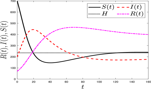
Figure 1: Populations of the SIR model (22) with $B(t)\equiv 12$, which is $R_{0}=B/(\mu H)=3.4043>1$.

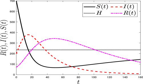
Figure 2: Populations of the SIR model (22) with $B(t)\equiv 3$, which is $R_{0}=B/(\mu H)=0.8511<1$.

6 SEIS Model

Consider $x(t):=[S(t),E(t),I(t)]^{T}\in\mathbb{R}_{+}^{3}$ governed by

$$\dot{S}= B-\mu S-\beta IS+\gamma I$$ (35a)

$$\dot{E}= \beta IS-\epsilon E-\mu E$$ (35b)

$$\dot{I}= \epsilon E-\gamma I-\mu I$$ (35c)

with $[S(0),E(0),I(0)]^{T}\in\mathbb{R}_{+}^{3}$ and $B:\mathbb{R}_{+}\to\mathbb{R}_{+}$. The equation (35) is referred to as the SEIS model KOROLyap04 . The SEIS model is known to be useful for describing diseases which have non-negligible incubation periods. The variable $E$ represents the (continuum) number of infected individuals who are not yet infectious. The SEIS model also consider infections which do not give long lasting immunity, and recovered individuals become susceptible again. As seen in (35), the short immunity forms a circle of length $3$, which the SIR model does not have.

The SEIS model (35) satisfies (6) and (8) with (23). Conditions (9) and (10) are satisfied. Thus Theorem 1 establishes ISS of the SEIS model (35) with respect to the input $B$, and an ISS Lyapunov function is obtained as (11) with $\lambda_{1}=\lambda_{2}=\lambda_{3}=1$, i.e., $V(x)=S+E+I=:N$. In fact, properties (24), (25) and (26) are verified.

For $x_{U}:=x=[S,E,I]^{T}$ and $V_{U}=V$, property (24) achieves (18) with $\alpha_{U}(s)=\mu s$ and $\sigma_{U}(s)=s$. EI-system consisting of (35b) and (35c) is iISS with respect to the input $S$ since the choice $V_{EI}=\log(1+E+I)$ satisfies

$$\dot{V}_{EI}\leq-\frac{\mu(E+I)}{1+E+I}+\beta S$$ (36)

along the solution $[E(t),I(t)]^{T}$ of EI-system. EI-system is, however, not ISS. EI-system is a Strongly iISS system admitting a zero local ISS-gain. To see this, one can make use of the Lyapunov function proposed in Theorem 1 by regarding $S$ as a constant $S^{\sharp}$ for EI-system. EI-system satisfies (6) and (8) with

$$\ell_{1,2}=\frac{\beta S^{\sharp}}{a(\gamma+\mu)},\quad\ell_{2,1}=\frac{\epsilon}{a(\epsilon+\mu)}$$ (37)

$$\theta_{1}(s)=(1\!-\!a)(\epsilon\!+\!\mu)s,\ \theta_{2}(s)=(1\!-\!a)(\gamma\!+\!\mu)s$$ (38)

for an arbitrarily given $a\in(0,1)$. Defining $V_{L}(x_{L})$ for $x_{L}=[E,I]^{T}$ as in (11) and (12) gives

$$V_{L}(x_{L})=E+\lambda_{2}I,\quad\lambda_{2}=\sqrt{\frac{\beta S^{\sharp}(\epsilon+\mu)}{(\gamma+\mu)\epsilon}}.$$ (39)

Then along the solution of (35b) and (35c) we obtain

$$\frac{d}{dt}V_{L}(x_{L})= \sqrt{\frac{\beta\epsilon(\epsilon+\mu)}{\gamma+\mu}}\left(\sqrt{S^{\sharp}}-\sqrt{\frac{(\gamma+\mu)(\epsilon+\mu)}{\beta\epsilon}}\right)E$$

$$+\sqrt{\beta^{2}S^{\sharp}}\left(\frac{S}{\sqrt{S^{\sharp}}}-\sqrt{\frac{(\gamma+\mu)(\epsilon+\mu)}{\beta\epsilon}}\right)I.$$ (40)

Define

$$H:=\frac{(\gamma+\mu)(\epsilon+\mu)}{\beta\epsilon}.$$ (41)

Equation (40) allows one to see that $S=H$ is a bifurcation point of EI-system. To this end, pick $S^{\sharp}=a^{2}H$. Due to $S\leq V_{U}(x_{U})$, EI-system satisfies (19) with (41) since such a parameter $a\in(0,1)$ can be taken for each $k\in(0,1)$. On the other hand, if $S$ is a constant satisfying $S>H$, equation (40) with $S^{\sharp}=S$ yields ${d}V_{L}(x_{L})/{dt}>0$ unless $E=I=0$. Therefore, EI-system is not ISS, but the convergence property (19) is met. Hence, Proposition 1 can be invoked for $Q=\mu H$, and concludes that

$$\sup_{s\in\mathbb{R}_{+}}{B}(t)<\mu H\ \Rightarrow\ \lim_{t\to\infty}\!E(t)=\lim_{t\to\infty}\!I(t)=0.$$ (42)

From (25), the solution $x(t)=[S(t),E(t),I(t)]^{T}$ of (35) satisfies (30) for any constant $B$. Accordingly, all the observations made for the SIR model apply to the SEIS model except that the increase of the infectious individuals $I$ is replaced by the increase of the weighted sum of infected individuals $E+\lambda_{2}I$. Simulations of the SEIS model (35) are shown in Figs. 3 and 4 for $\beta=0.0002$, $\mu=0.015$ and $\gamma=0.032$ with $S(0)=700$, $I(0)=200$ and $R(0)=70$. The thresholds are $H=455.3$ and $\mu H=6.83$. The disease is removed in Fig. 4 plotted for $B=3<\mu H$. The infected and infectious populations remain high in Fig. 3 computed for $B=12>\mu H$.

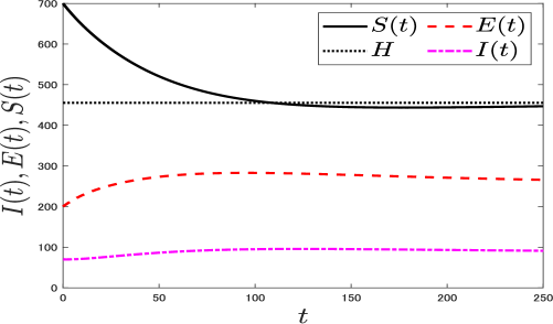
Figure 3: Populations of the SEIS model (35) with $B(t)\equiv 12$, which is $R_{0}=B/(\mu H)=1.757>1$.

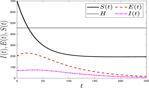
Figure 4: Populations of the SEIS model (35) with $B(t)\equiv 3$, which is $R_{0}=B/(\mu H)=0.4393<1$.

7 MSIR and SEIR Models

Consider $x(t):=[M(t),S(t),I(t),R(t)]^{T}\in\mathbb{R}_{+}^{4}$ for

$$\dot{M}= B-\delta M-\mu M$$ (43a)

$$\dot{S}= \delta M-\mu S-\beta IS$$ (43b)

$$\dot{I}= \beta IS-\gamma I-\mu I$$ (43c)

$$\dot{R}= \gamma I-\mu R$$ (43d)

which is called the MSIR model HETHinfdiseas ; MCLANDmsirID88 . The variable $M$ represents delay in becoming susceptible due to the maternally derived immunity. The analysis of the MSIR model is almost the same as that of the SIR model. With

$$\ell_{i+1,i}=\ell_{i,i+1}=1,\ \theta_{i}(s)=\mu s,\ i=1,2,3,4,$$ (44)

Theorem 1 assures that the function $N(t):=M(t)+S(t)+I(t)+R(t)$ proves ISS of (43), and the ultimate bounds (25) and (26) via (24). Thus, the choices $V_{U}(x)=N$ and $x=x_{U}$ give (18) with $\alpha_{U}(s)=\mu s$ and $\sigma_{U}(s)=s$. Because of the bilinear term $\beta IS$, I-system in (43) is not ISS, but Strongly iISS. Thus, the variable $I(t)$ increases until $S(t)\leq H$, where the bifurcation point $H$ is defined as (27). The ISS gain of I-system is zero for the input $\sup_{s\in\mathbb{R}_{+}}S(t)<H$. In fact, I-system satisfies (19). Thus, Proposition 1 establishes

$${B}<\mu H\ \Rightarrow\ \lim_{t\to\infty}x(t)=\left[\frac{B}{\mu},0,0,0\right]^{T}$$ (45)

for the MSIR model (43) in the case of constant $B\in\mathbb{R}_{+}$.

Finally, the SEIR model consists of

$$\dot{S}= B-\mu S-\beta IS$$ (46a)

$$\dot{E}= \beta IS-\epsilon E-\mu E$$ (46b)

$$\dot{I}= \epsilon E-\gamma I-\mu I$$ (46c)

$$\dot{R}= \gamma I-\mu R.$$ (46d)

Its state vector is $x(t):=[S(t),E(t),I(t),R(t)]^{T}\in\mathbb{R}_{+}^{4}$ LIMULDseirlyapu95 . The SEIR model can be analyzed as done for the SIES model. Theorem 1 qualifies $N(t):=S(t)+E(t)+I(t)+R(t)$ as an ISS Lyapunov function proving ISS of (46), and provides the ultimate bounds (25) and (26) via (24). Property (18) holds with $\alpha_{U}(s)=\mu s$ and $\sigma_{U}(s)=s$ for $V_{U}(x)=N$ and $x=x_{U}$. EIR-system consisting of (46b), (46c) and (46d) is Strongly iISS with respect to the input $S$, although the bilinear term $\beta IS$ prevent it from being ISS. Using $V_{L}(x_{L})=\lambda_{E}E+\lambda_{I}I+\lambda_{R}R$ for appropriate $\lambda_{E}$, $\lambda_{I}$, $\lambda_{R}>0$ given by Theorem 1, one can show that EIR-system is not ISS. The function $V_{L}(x_{L})$ also shows that EIR-system admits the zero ISS gain for the input $\sup_{s\in\mathbb{R}_{+}}S(t)<H$, where the bifurcation point $H$ is defined as (41). EIR-system satisfies (19). Therefore, Proposition 1 concludes that the SEIR model (46) satisfies (45) for constant $B\in\mathbb{R}_{+}$.

8 Vaccination models

One way of eradicating infectious diseases is to vaccinate newborns and entering individuals. Let the constant $P\in(0,1)$ denote the vaccination fraction. Considering a vaccine giving lifelong immunity HETHinfdiseas , the SIR model can be modified as

$$\dot{S}= B(1-P)-\mu S-\beta IS$$ (47a)

$$\dot{I}= \beta IS-\gamma I-\mu I$$ (47b)

$$\dot{R}= \gamma I-\mu R$$ (47c)

$$\dot{A}= BP-\mu A,$$ (47d)

where $A$ is the number of vaccinated individuals. Since (8) is satisfied with (44), Theorem 1 assures that $N(t):=S(t)+I(t)+R(t)+A(t)$ is an ISS Lyapunov function for the model (47), and establishes the ultimate bounds (25) and (26) via (24). S-system is ISS with respect to the input $B$. In fact, property (18) is met with $V_{U}(x_{U})=S$, $x_{U}=S$, $\alpha_{U}(s)=\mu s$ and $\sigma_{U}(s)=(1-P)s$. IR system is the same as that of the SIR model. Hence, a bifurcation point $H$ is obtained as (27). The convergence of $I$ to zero implies $\lim_{t\to\infty}R(t)=0$. The variable $A$ reaches its steady state since $A$-system is ISS. Indeed, Hence, Proposition 1 guarantees

$${B}(1\!-\!P)<\mu H\ \Rightarrow\ \lim_{t\to\infty}x(t)=\left[\frac{B(1\!-\!P)}{\mu},0,0,\frac{BP}{\mu}\right]^{T}$$ (48)

for any constant $B\in\mathbb{R}_{+}$ and $P\in(0,1)$. Hence, a vaccination fraction $P$ which is sufficiently close to $1$ can eradicate the disease.

Another way to model the newborn vaccination within the SIR model is

$$\dot{S}= B(1-P)-\mu S-\beta IS$$ (49a)

$$\dot{I}= \beta IS-\gamma I-\mu I$$ (49b)

$$\dot{R}= \gamma I-\mu R+BP.$$ (49c)

Assumption (8) is satisfied with (23), Theorem 1 proves ISS of (49) with $N(t):=S(t)+I(t)+R(t)$, which establishes (25) and (26) via (24). The reminder of the analysis is the same as that of the model (47) except that the convergence of $I$ to zero does not imply $\lim_{t\to\infty}R(t)=0$. Since the scalar $R$-system is ISS, it is clear that

$${B}(1-P)<\mu H\ \Rightarrow\ \lim_{t\to\infty}x(t)=\left[\frac{B(1-P)}{\mu},0,\frac{BP}{\mu}\right]^{T}$$ (50)

for any constant $B\in\mathbb{R}_{+}$ and $P\in(0,1)$.

The same modifications to other disease models in the previous sections can be possible for modeling the newborn vaccination DLsencontrdiseas12 . Their analysis goes in essentially the same way as the one described above for the SIR model.

If non-newborns/non-immigrants are vaccinated OGR_IDGoptivacci02 ; ZAM_IDSIRvacci08 , a way to modify the SIR model is

$$\dot{S}= B-\rho S-\mu S-\beta IS$$ (51a)

$$\dot{I}= \beta IS-\gamma I-\mu I$$ (51b)

$$\dot{R}= \gamma I-\mu R$$ (51c)

$$\dot{A}= \rho S-\mu A,$$ (51d)

where the constant $\rho\in\mathbb{R}_{+}$ is the vaccination rate. The analysis is the same as that of (47) except that ISS of S-system with respect to the input $B$ yields property (18) with $V_{U}(x_{U})=S$, $x_{U}=S$ for $\alpha_{U}(s)=(\rho+\mu)s$ and $\sigma_{U}(s)=s$. Hence,

$${B}<(\rho+\mu)H\ \Rightarrow\ \lim_{t\to\infty}x(t)=\left[\frac{B(1\!-\!P)}{\mu},0,0,\frac{BP}{\mu}\right]^{T}$$ (52)

for any constant $B\in\mathbb{R}_{+}$ and $\rho\in\mathbb{R}_{+}$. Thus, the disease can be eradicated by a sufficiently high vaccination rate $\rho$. Irrespective of ${B}<(\rho+\mu)H$, the ultimate bounds (25) and (26) hold, and the model (51) also has the bifurcation point at $S=H$ given in (27).

9 Concluding Remarks

This paper has investigated popular models of infectious diseases from the viewpoint of iISS and ISS. It has been shown that behavior of all the models can be analyzed uniformly in terms of a asymptotic gain property of ISS, and a Strongly iISS component which is not globally ISS, but admits a zero local ISS-gain function. The outbreak is caused by the Strongly iISS component which is not ISS. However, the disease is eradicable since the Strongly iISS component possesses zero local ISS-gain which takes effect if a characteristic value is below a threshold. The notions of (i)ISS absorb changes of equilibria, and provide a module-based framework. The analysis of global properties does not require direct and heuristic construction of different Lyapunov functions of the entire network depending on equilibria. This demonstration is the main contribution of this paper. The same procedure and explanation are valid even in the presence of an outer-loop caused by short-time immunity. The source of the particular iISS component is bilinearity. Indeed, scalar linear systems can never exhibit peaks, the outbreak. Although the bilinearity is the only nonlinearity in the popular simplest models, the theoretical tools presented in this paper accommodate a broad class of nonlinearities, such as saturation, non-monotone nonlinearities CAPSERgennonID78 ; LIULEVgennonID86 ; KOROgennonID06 ; XIARUAgennonID07 ; EnaNakIDlyapdelay11 ; EnaNakIDlyap14 and others, as long as component models retain appropriate iISS and ISS properties. In fact, the arguments in this paper rely on neither linearity nor particular nonlinearities. Only ISS, iISS and ISS-gain characterizations are utilized.

This paper has not reported new epidemiologic discoveries. Nevertheless, the system and signal treatment is expected to be superior to heuristic approaches in finding control strategies for eradicating or containing the spread of diseases. The proposed option aims to facilitate the research on control design with global guarantees. It is worth noticing that Lyapunov functions used in this paper are weighted sum of populations, which are simpler than logarithmic functions that have been popular in the field of mathematical epidemiology KOROLyap02 . More importantly, (i)ISS Lyapunov functions constructed in this paper are different from Lyapunov functions in the conventional concept, and the construction of Lyapunov functions does not need preprocessing of equilibria. The vaccination discussed in this paper is open-loop. Interesting future research includes introduction of the (i)ISS framework to closed-loop control design (see, e.g., NIEfcimpulseID12 ; DLsencontrdiseas12 ; ALQoutlinzdiseas12 and references therein).

References

- (1) S. Alonso-Quesada, M. De la Sen, RP. Agarwal, A. Ibeas (2012), An observer-based vaccination control law for an SEIR epidemic model based on feedback linearization techniques for nonlinear systems. Adv. Differ. Equ. 2012:161
- (2) R.M. Anderson, R.M. May (1979) Population biology of infectious diseases: Part I. Nature 280:361–367
- (3) D. Angeli, A. Astolfi (2007) A tight small gain theorem for not necessarily ISS systems. Syst. Control Lett. 56:87–91
- (4) D. Angeli, E.D. Sontag, Y. Wang (2000) A characterization of integral input-to-state stability. IEEE Trans. Autom. Control 45(6):1082–1097
- (5) V. Capasso, G. Serio (1978) A generalization of the Kermack-McKendrick deterministic epidemic model. Math. Biosci. 42:43–61
- (6) A. Chaillet, D. Angeli (2008) Integral input to state stable systems in cascade. Syst. Control Lett. 57:519–527
- (7) A. Chaillet, D. Angeli, H. Ito (2014) Combining iISS and ISS with respect to small inputs: the Strong iISS property. IEEE Trans. Automat. Contr. 59(9):2518–2524
- (8) A. Chaillet, D. Angeli, H. Ito (2014) Strong iISS is preserved under cascade interconnection. Automatica 50(9):2424–2427
- (9) Y. Chen, J. Yang, F. Zhang (2014) The global stability of an SIRS model with infection age. Math. Biosci. Eng. 11:449–469
- (10) S. Dashkovskiy, H. Ito, F. Wirth (2011) On a small-gain theorem for ISS networks in dissipative Lyapunov form. European J. Contr. 17, 357–365
- (11) S. Dashkovskiy, B.S. Rüffer, F.R. Wirth (2010) Small gain theorems for large scale systems and construction of ISS Lyapunov functions. SIAM J. Control Optim. 48:4089–4118
- (12) M. De la Sen, A. Ibeas, S. Alonso-Quesada (2012) On vaccination controls for the SEIR epidemic model. Commun. Nonlinear Sci. Numer. Simul. 17(6):2637–2658
- (13) Y. Enatsu, Y. Nakata (2014) Stability and bifurcation analysis of epidemic models with saturated incidence rates: an application to a nonmonotone incidence rate. Math. Biosci. Eng. 11:78-5-805
- (14) Y. Enatsu, Y. Nakata, Y. Muroya (2011) Global stability of SIR epidemic models with a wide class of nonlinear incidence rates and distributed delays. Disc. Cont. Dynam. Sys. B 15:61–74
- (15) A. Fall, A. Iggidr, G. Sallet, J. J. Tewa (2007) Epidemiological models and Lyapunov functions. Math. Model. Nat. Phenom. 2(1):62–83
- (16) H.W. Hethcote (2000) The mathematics of infectious diseases. SIAM Rev. 42(4):599–653
- (17) H. Ito (2006) State-dependent scaling problems and stability of interconnected iISS and ISS systems. IEEE Trans. Autom. Control 51(10):1626–1643
- (18) H. Ito (2010) A Lyapunov approach to cascade interconnection of integral input-to-state stable systems. IEEE Trans. Autom. Control 55(3):702–708
- (19) H. Ito (2017) Relaxing growth rate assumption for integral input-to-state stability of cascade systems. In: Proceedings of the SICE Annual Conference 2017, pp 689–694
- (20) H. Ito (2020) Strong integral input-to-state stability of nonlinear networks through balancing kinetics. submitted to the 59th IEEE Conf. Decision Control
- (21) H. Ito, Z.P. Jiang (2009) Necessary and sufficient small gain conditions for integral input-to-state stable systems: A Lyapunov perspective. IEEE Trans. Autom. Contorl 54:2389–2404
- (22) H. Ito, Z.P. Jiang, S. Dashkovskiy, B.S. Rüffer (2013) Robust stability of networks of iISS systems: construction of sum-type Lyapunov functions. IEEE Trans. Autom. Control 58:1192–1207
- (23) Z.P. Jiang, I. Mareels, Y. Wang (1996) A Lyapunov formulation of the nonlinear small-gain theorem for interconnected ISS systems. Automatica 32:1211–1215
- (24) I. Karafyllis, Z.P. Jiang (2011) A vector small-gain theorem for general nonlinear control systems. IMA J. Math. Control Info. 28(3):309–344
- (25) M.J. Keeling, P. Rohani (2008) Modeling infectious diseases in humans and animals, Princeton Univ. Press, Princeton
- (26) W.O. Kermack, A.G. McKendrick (1927) A contribution to the mathematical theory of epidemics.” Proc. R. Soc. Lond. A115:700–721
- (27) A. Korobeinikov (2004) Lyapunov functions and global properties for SEIR and SEIS epidemic models. Math. Med. Biol. 21:75–83
- (28) A. Korobeinikov (2006) Lyapunov functions and global stability for SIR and SIRS epidemiological models with non-linear transmission. Bulletin Math. Biol. 30:615-–626
- (29) A. Korobeinikov, G.C. Wake (2002) Lyapunov functions and global stability for SIR, SIRS, and SIS epidemiological models, Appl. Math. Lett. 15:955-960
- (30) M.Y. Li, J.S. Muldowney (1995) Global stability for the SEIR model in epidemiology. Math. Biosci. 125:155–164
- (31) T. Liu, D.J. Hill, Z.P. Jiang (2011) Lyapunov formulation of ISS small-gain in continuous-time dynamical networks. Automatica 47:2088–2093
- (32) W.M. Liu, S.A. Levin, Y. Iwasa (1986) Influence of nonlinear incidence rates upon the behavior of SIRS epidemiological models. J. Math. Biol. 23:187–204
- (33) A.R. McLean, R.M. Anderson (1988) Measles in developing countries Part I. Epidemiological parameters and patterns. Epidemiology and Infection 100:111–133
- (34) Y. Nakata, Y. Enatsu, H. Inaba, T. Kuniya, Y. Muroya,, Y. Takeuchi (2014) Stability of epidemic models with waning immunity. SUT J. Mathematics 50(2):205-–245
- (35) L.F. Nie, Z.D. Teng, A. Torres (2012) Dynamic analysis of an SIR epidemic model with state dependent pulse vaccination. Nonlinear Anal., Real World Appl. 13(4):1621–1629
- (36) P. Ogren, C.F. Martin (2002) Vaccination strategies for epidemics in highly mobile populations. Appl. Math. Comput. 127:261–276
- (37) S.M. O’Regan, T.C. Kelly, A. Korobeinikov, M.J.A. O’Callaghan, A.V. Pokrovskii (2010) Lyapunov functions for SIR and SIRS epidemic models. Appl. Math. Lett 23(4):446–448
- (38) Z. Shuai, P. van den Driessche (2013) Global stability of infectious disease models using Lyapunov functions. SIAM J. Appl. Math. 73(4):1513–1532
- (39) E.D. Sontag (1989) Smooth stabilization implies coprime factorization. IEEE Trans. Autom. Control 34(4):435–443
- (40) E.D. Sontag (1998) Comments on integral variants of ISS. Syst. Control Lett. 34(1-2):93–100
- (41) E.D. Sontag (2008) Input to state stability: basic concepts and results. In: Nistri P., Stefani G. (eds) Nonlinear and optimal control theory. Springer, Berlin, pp 163–220
- (42) E.D. Sontag, Y. Wang (1995) On characterizations of input-to-state stability property. Syst. Control Lett. 24(5):351–359
- (43) D. Xiao, S. Ruan (2007) Global analysis of an epidemic model with nonmonotone incidence rate. Math. Biosci. 208:419–429
- (44) G. Zaman, Y.H. Kang, I.H. Jung (2008) Stability analysis and optimal vaccination of an SIR epidemic model. Biosystems 93(3):240–249