1 Introduction
Our convention in this paper is that the ( n , m ) 𝑛 𝑚 (n,m) G = ( V ( G ) , E ( G ) ) 𝐺 𝑉 𝐺 𝐸 𝐺 G=(V(G),E(G)) n 𝑛 n m 𝑚 m [1 ] . One of the most critical fields in the graph theory is spectral graph theory. In particular, spectral graph theory is consist of algebraic spectral graph theory and analytic spectral graph theory. Spectral graph theory not only have pure mathematics properties, but also several vital applications in practical, examples include information-theoretic hashing of 3D objects[2 ] , threshold selection in gene co-expression networks[3 ] , pattern recognition, data mining and image matching[4 ] . Thus, it is of great interests to determine the spectra of some graphs, especially for those large graphs which resulted from the small graph by graph operations in past two decades. For adjacency and Laplacian spectra of certain graph operations, see [5 , 6 , 7 , 8 , 9 , 10 , 11 , 12 , 13 , 14 , 15 , 16 , 17 , 18 ] and references therein. Alone this line, we consider the normalized Laplacian spectra of two parallel subdivision graphs in this paper, see Figure 1.
It is worthy to mentioned that S 1 ( G ) subscript 𝑆 1 𝐺 S_{1}(G) S ( G ) 𝑆 𝐺 S(G) k = 1 𝑘 1 k=1 S k ( G ) subscript 𝑆 𝑘 𝐺 S_{k}(G) [19 ] . Besides, S 2 ( G ) subscript 𝑆 2 𝐺 S_{2}(G) [20 ] if k = 2 𝑘 2 k=2 S k ( G ) subscript 𝑆 𝑘 𝐺 S_{k}(G) k = 1 𝑘 1 k=1 G 𝐺 G S 2 k ( G ) subscript 𝑆 2 𝑘 𝐺 S_{2k}(G) S 2 ( G ) subscript 𝑆 2 𝐺 S_{2}(G) [21 ] .
In what follows, we will recall the definition of the normalized Laplacian. The formal definition is defined as
ℒ ( G ) = { − w ( i , j ) d ( i ) d ( j ) , i is adjacent to j ; d ( i ) − w ( i , i ) d ( i ) , i = j , d ( i ) ≠ 0 ; 0 , otherwise. ℒ 𝐺 cases 𝑤 𝑖 𝑗 𝑑 𝑖 𝑑 𝑗 i is adjacent to j ; 𝑑 𝑖 𝑤 𝑖 𝑖 𝑑 𝑖 i = j , d ( i ) ≠ 0 ; 0 otherwise. \displaystyle\mathscr{L}(G)=\left\{\begin{array}[]{ll}\frac{-w(i,j)}{\sqrt{d(i)d(j)}},&\hbox{$i$ is adjacent to $j$;}\\
\frac{d(i)-w(i,i)}{d(i)},&\hbox{$i=j,d(i)\neq 0$;}\\
~{}~{}~{}~{}~{}~{}0,&\hbox{otherwise.}\end{array}\right.
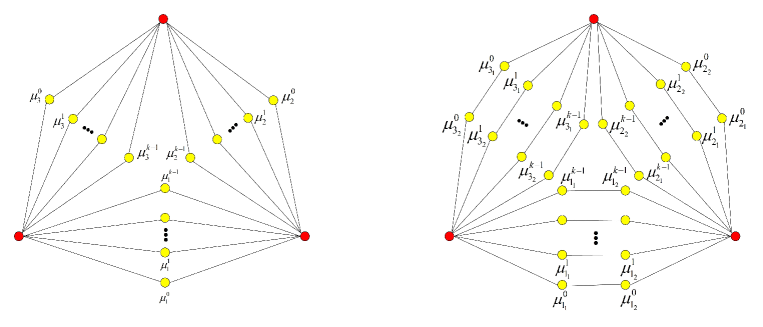
Figure 1: (a) S k ( G ) subscript 𝑆 𝑘 𝐺 S_{k}(G) S 2 k ( G ) subscript 𝑆 2 𝑘 𝐺 S_{2k}(G)
In the definition defined as above, w ( i , j ) 𝑤 𝑖 𝑗 w(i,j) i j 𝑖 𝑗 ij w ( i , u ) 𝑤 𝑖 𝑢 w(i,u) w ( i , j ) = 1 𝑤 𝑖 𝑗 1 w(i,j)=1 w ( i , i ) = 0 𝑤 𝑖 𝑖 0 w(i,i)=0
ℒ ( G ) = { − 1 d ( i ) d ( j ) , i is adjacent to j ; 1 , i = j , d ( i ) ≠ 0 ; 0 , else. ℒ 𝐺 cases 1 𝑑 𝑖 𝑑 𝑗 i is adjacent to j ; 1 i = j , d ( i ) ≠ 0 ; 0 else. \displaystyle\mathscr{L}(G)=\left\{\begin{array}[]{ll}\frac{-1}{\sqrt{d(i)d(j)}},&\hbox{$i$ is adjacent to $j$;}\\
~{}~{}~{}~{}~{}~{}1,&\hbox{$i=j,d(i)\neq 0$;}\\
~{}~{}~{}~{}~{}~{}0,&\hbox{else.}\end{array}\right. (1.5)
Apparently, one has ℒ ( G ) = D ( G ) − 1 2 L ( G ) D ( G ) − 1 2 ℒ 𝐺 𝐷 superscript 𝐺 1 2 𝐿 𝐺 𝐷 superscript 𝐺 1 2 \mathscr{L}(G)=D(G)^{-\frac{1}{2}}L(G)D(G)^{-\frac{1}{2}}
Recent years, Xie and Zhang [22 , 19 ] respectively determined the normalized Laplacians of subdivisions and iterated triangulations graph. In 2017, the normalized Laplacians for quadrilateral graphs are considered by Li and Hou[23 ] . Pan et al.[24 ] computed the
normalized Laplacians of some graphs which involve graph transformations. For details, see [25 , 26 , 27 , 28 , 29 , 30 ] and references therein.
A topic of a good deal of attention in network science is the notion of network criticality. some measures for network criticality are
depended on the paths in networks. Thus the shortest paths in networks are the focus of attention while we compute network criticality. But
the shortest paths are not considering the impacts of all the paths. The concepts of resistance distance and Kirchhoff index are such measures which involving all the information among paths in networks, one may refer to [31 ] .
Resistance distance [32 ] is defined by Klein and Randić. Denote Ω i j subscript Ω 𝑖 𝑗 \Omega_{ij} i 𝑖 i j 𝑗 j [33 ] , Klein et al. defined the resistance distance sum rules, which is Kirchhoff index K f ( G ) 𝐾 𝑓 𝐺 Kf(G) [34 ] defined the multiplicative degree Kirchhoff index K f ∗ ( G ) 𝐾 superscript 𝑓 𝐺 Kf^{*}(G) K f ∗ ( G ) 𝐾 superscript 𝑓 𝐺 Kf^{*}(G) ℒ ( G ) ℒ 𝐺 \mathscr{L}(G)
The hitting time or first passage time T j subscript 𝑇 𝑗 T_{j} j 𝑗 j i 𝑖 i E i T j ( G ) subscript 𝐸 𝑖 subscript 𝑇 𝑗 𝐺 E_{i}T_{j}(G) C u v ( G ) subscript 𝐶 𝑢 𝑣 𝐺 C_{uv}(G) i 𝑖 i j 𝑗 j i 𝑖 i G 𝐺 G K e ( G ) 𝐾 𝑒 𝐺 Ke(G) G 𝐺 G G 𝐺 G [35 , 36 ] .
For a general graph, it is hard enough to determine the resistance distance between any points, unless the graph is very small or one knows the complete information of the graph. A. K. Chandra et al. in [37 ] built a relation between the expected hitting time and resistance distance of a graph. This provides a available method to calculate any two-points resistance distance, see[38 , 39 , 40 , 41 , 42 ] . The main results of this paper are presented as below.
1.1 The normalized Laplacian of S k ( G ) subscript 𝑆 𝑘 𝐺 S_{k}(G)
In this subsection, we will give the complete information for the normalized Laplacian of the k 𝑘 k
f 1 ( x ) = 2 + 4 − 2 x 2 , f 2 ( x ) = 2 − 4 − 2 x 2 . formulae-sequence subscript 𝑓 1 𝑥 2 4 2 𝑥 2 subscript 𝑓 2 𝑥 2 4 2 𝑥 2 \displaystyle f_{1}(x)=\frac{2+\sqrt{4-2x}}{2},~{}f_{2}(x)=\frac{2-\sqrt{4-2x}}{2}.
Theorem 1.1 .
Assume that G 𝐺 G ( n , m ) 𝑛 𝑚 (n,m) ℒ ( S k ( G ) ) ℒ subscript 𝑆 𝑘 𝐺 \mathscr{L}(S_{k}(G))
•
f 1 ( λ ) subscript 𝑓 1 𝜆 f_{1}(\lambda) f 2 ( λ ) subscript 𝑓 2 𝜆 f_{2}(\lambda) ℒ ( S k ( G ) ) ℒ subscript 𝑆 𝑘 𝐺 \mathscr{L}(S_{k}(G)) λ ( λ ≠ 0 ) 𝜆 𝜆 0 \lambda(\lambda\neq 0) ℒ ( G ) . ℒ 𝐺 \mathscr{L}(G). f 1 ( λ ) subscript 𝑓 1 𝜆 f_{1}(\lambda) f 2 ( λ ) subscript 𝑓 2 𝜆 f_{2}(\lambda) λ 𝜆 \lambda
•
0 0 2 2 2 ℒ ( S k ( G ) ) ℒ subscript 𝑆 𝑘 𝐺 \mathscr{L}(S_{k}(G)) 1 1 1
•
ℒ ( S k ( G ) ) ℒ subscript 𝑆 𝑘 𝐺 \mathscr{L}(S_{k}(G)) k m − n + 2 𝑘 𝑚 𝑛 2 km-n+2 G 𝐺 G k m − n 𝑘 𝑚 𝑛 km-n
1.2 The normalized Laplacian of S 2 k ( G ) subscript 𝑆 2 𝑘 𝐺 S_{2k}(G)
In this subsection, the normalized Laplacian eigenvalues of the 2 k 2 𝑘 2k μ 1 , subscript 𝜇 1 \mu_{1}, μ 2 subscript 𝜇 2 \mu_{2} μ 3 subscript 𝜇 3 \mu_{3} 4 μ 3 − 12 μ 2 + 9 μ − λ = 0 4 superscript 𝜇 3 12 superscript 𝜇 2 9 𝜇 𝜆 0 4\mu^{3}-12\mu^{2}+9\mu-\lambda=0
Theorem 1.2 .
Assume that G 𝐺 G ( n , m ) 𝑛 𝑚 (n,m) ℒ ( S 2 k ( G ) ) ℒ subscript 𝑆 2 𝑘 𝐺 \mathscr{L}(S_{2k}(G))
•
μ 1 , subscript 𝜇 1 \mu_{1}, μ 2 subscript 𝜇 2 \mu_{2} μ 3 subscript 𝜇 3 \mu_{3} ℒ ( S 2 k ( G ) ) ℒ subscript 𝑆 2 𝑘 𝐺 \mathscr{L}(S_{2k}(G)) λ ( λ ≠ 0 , 2 ) 𝜆 𝜆 0 2
\lambda(\lambda\neq 0,2) ℒ ( G ) . ℒ 𝐺 \mathscr{L}(G). μ 1 , subscript 𝜇 1 \mu_{1}, μ 2 subscript 𝜇 2 \mu_{2} μ 3 subscript 𝜇 3 \mu_{3} λ 𝜆 \lambda
•
ℒ ( S 2 k ( G ) ) ℒ subscript 𝑆 2 𝑘 𝐺 \mathscr{L}(S_{2k}(G)) 0 0 1 1 1 ℒ ( S 2 k ( G ) ) ℒ subscript 𝑆 2 𝑘 𝐺 \mathscr{L}(S_{2k}(G)) 2 2 2 1 1 1 G 𝐺 G
•
ℒ ( S 2 k ( G ) ) ℒ subscript 𝑆 2 𝑘 𝐺 \mathscr{L}(S_{2k}(G)) 1 2 1 2 \frac{1}{2} 3 2 3 2 \frac{3}{2} k m − n 𝑘 𝑚 𝑛 km-n k m − n + 2 𝑘 𝑚 𝑛 2 km-n+2 G 𝐺 G
•
ℒ ( S 2 k ( G ) ) ℒ subscript 𝑆 2 𝑘 𝐺 \mathscr{L}(S_{2k}(G)) 1 2 1 2 \frac{1}{2} 3 2 3 2 \frac{3}{2} k m − n + 2 𝑘 𝑚 𝑛 2 km-n+2 G 𝐺 G
The rest parts are summarized as below. We propose some lemmas in section 2. The proofs of the main results are provided in section 3. The spectra of ℒ ( S k ( G ) ) ℒ subscript 𝑆 𝑘 𝐺 \mathscr{L}(S_{k}(G)) ℒ ( S 2 k ( G ) ) ℒ subscript 𝑆 2 𝑘 𝐺 \mathscr{L}(S_{2k}(G)) E i T j ( S k ( G ) ) subscript 𝐸 𝑖 subscript 𝑇 𝑗 subscript 𝑆 𝑘 𝐺 E_{i}T_{j}(S_{k}(G)) r i j ( S k ( G ) ) subscript 𝑟 𝑖 𝑗 subscript 𝑆 𝑘 𝐺 r_{ij}(S_{k}(G)) K f ∗ ( S k ( G ) ) 𝐾 superscript 𝑓 subscript 𝑆 𝑘 𝐺 Kf^{*}(S_{k}(G)) K f ∗ ( S 2 k ( G ) ) 𝐾 superscript 𝑓 subscript 𝑆 2 𝑘 𝐺 Kf^{*}(S_{2k}(G)) K e ( S k ( G ) ) 𝐾 𝑒 subscript 𝑆 𝑘 𝐺 Ke(S_{k}(G)) K f ∗ ( S 2 k ( G ) ) 𝐾 superscript 𝑓 subscript 𝑆 2 𝑘 𝐺 Kf^{*}(S_{2k}(G)) τ ( S k ( G ) ) 𝜏 subscript 𝑆 𝑘 𝐺 \tau(S_{k}(G)) τ ( S 2 k ( G ) ) 𝜏 subscript 𝑆 2 𝑘 𝐺 \tau(S_{2k}(G))
2 Preliminaries
In this section, we put some lemmas that used in applications section. Let 0 = λ 1 < λ 2 ≤ ⋯ ≤ λ n 0 subscript 𝜆 1 subscript 𝜆 2 ⋯ subscript 𝜆 𝑛 0=\lambda_{1}<\lambda_{2}\leq\cdots\leq\lambda_{n} ℒ ( G ) ℒ 𝐺 \mathscr{L}(G)
In 2007, Chen and Zhang found that K f ∗ ( G ) 𝐾 superscript 𝑓 𝐺 Kf^{*}(G) ℒ ( S k ( G ) ) ℒ subscript 𝑆 𝑘 𝐺 \mathscr{L}(S_{k}(G)) G 𝐺 G
Lemma 2.1 .
[ 34 ] Assume that G 𝐺 G ( n , m ) 𝑛 𝑚 (n,m) K f ∗ ( G ) = 2 m ∑ i = 2 n 1 λ i . 𝐾 superscript 𝑓 𝐺 2 𝑚 superscript subscript 𝑖 2 𝑛 1 subscript 𝜆 𝑖 Kf^{*}(G)=2m\sum_{i=2}^{n}\frac{1}{\lambda_{i}}.
Kemeny and Snell in 1960 introduced the graph invariant which is called Kemeny’s constant. It also related to the eigenvalues of ℒ ( S k ( G ) ) ℒ subscript 𝑆 𝑘 𝐺 \mathscr{L}(S_{k}(G))
Lemma 2.2 .
[ 30 ] Assume that G 𝐺 G ( n , m ) 𝑛 𝑚 (n,m) K e ( G ) = ∑ i = 2 n 1 λ i . 𝐾 𝑒 𝐺 superscript subscript 𝑖 2 𝑛 1 subscript 𝜆 𝑖 Ke(G)=\sum_{i=2}^{n}\frac{1}{\lambda_{i}}.
Combining Lemmas 2.1 and 2.2, one finds K f ∗ ( G ) = 2 m ⋅ K e ( G ) 𝐾 superscript 𝑓 𝐺 ⋅ 2 𝑚 𝐾 𝑒 𝐺 Kf^{*}(G)=2m\cdot Ke(G) B ( G ) 𝐵 𝐺 B(G) r ( B ( G ) ) 𝑟 𝐵 𝐺 r(B(G)) B ( G ) 𝐵 𝐺 B(G)
Lemma 2.3 .
[ 30 ] Assume that G 𝐺 G ( n , m ) 𝑛 𝑚 (n,m)
r ( B ( G ) ) = { n , if G is non-bipartite; n − 1 , if G is bipartite. 𝑟 𝐵 𝐺 cases 𝑛 if G is non-bipartite; 𝑛 1 if G is bipartite. \displaystyle r(B(G))=\left\{\begin{array}[]{ll}n,&\hbox{if $G$ is non-bipartite;}\\
n-1,&\hbox{if $G$ is bipartite.}\end{array}\right.
Lemma 2.4 .
[ 43 ] Assume that G 𝐺 G ( n , m ) 𝑛 𝑚 (n,m)
∏ i = 1 n d ( v i ) ∏ i = 2 n λ i = 2 m τ ( G ) , superscript subscript product 𝑖 1 𝑛 𝑑 subscript 𝑣 𝑖 superscript subscript product 𝑖 2 𝑛 subscript 𝜆 𝑖 2 𝑚 𝜏 𝐺 \displaystyle\prod_{i=1}^{n}d(v_{i})\prod_{i=2}^{n}\lambda_{i}=2m\tau(G),
where
τ ( G ) 𝜏 𝐺 \tau(G) G 𝐺 G
At this point, one considers the normalized adjacency matrix N ( G ) 𝑁 𝐺 N(G)
N ( G ) = D ( G ) − 1 2 A ( G ) D ( G ) − 1 2 = D ( G ) 1 2 ( I − ℒ ( G ) ) D ( G ) − 1 2 , 𝑁 𝐺 𝐷 superscript 𝐺 1 2 𝐴 𝐺 𝐷 superscript 𝐺 1 2 𝐷 superscript 𝐺 1 2 𝐼 ℒ 𝐺 𝐷 superscript 𝐺 1 2 \displaystyle N(G)=D(G)^{-\frac{1}{2}}A(G)D(G)^{-\frac{1}{2}}=D(G)^{\frac{1}{2}}(I-\mathscr{L}(G))D(G)^{-\frac{1}{2}},
where I 𝐼 I
The above equation leads that matrix N ( G ) 𝑁 𝐺 N(G) I − ℒ ( G ) 𝐼 ℒ 𝐺 I-\mathscr{L}(G) I − ℒ ( G ) 𝐼 ℒ 𝐺 I-\mathscr{L}(G) v 1 , v 2 , … , v n subscript 𝑣 1 subscript 𝑣 2 … subscript 𝑣 𝑛
v_{1},v_{2},\ldots,v_{n}
v i = ( v i 1 , v i 2 , … , v i n ) T , i = 1 , 2 , … , n . formulae-sequence subscript 𝑣 𝑖 superscript subscript 𝑣 𝑖 1 subscript 𝑣 𝑖 2 … subscript 𝑣 𝑖 𝑛 𝑇 𝑖 1 2 … 𝑛
v_{i}=(v_{i1},v_{i2},\ldots,v_{in})^{T},~{}i=1,2,\ldots,n.
One knows that E = ( v 1 , v 2 , … , v n ) 𝐸 subscript 𝑣 1 subscript 𝑣 2 … subscript 𝑣 𝑛 E=(v_{1},v_{2},\ldots,v_{n})
∑ k = 1 n v i k v j k = ∑ k = 1 n v k i v k j = { 1 , if i = j ; 0 , else. superscript subscript 𝑘 1 𝑛 subscript 𝑣 𝑖 𝑘 subscript 𝑣 𝑗 𝑘 superscript subscript 𝑘 1 𝑛 subscript 𝑣 𝑘 𝑖 subscript 𝑣 𝑘 𝑗 cases 1 if i = j ; 0 else. \displaystyle\sum_{k=1}^{n}v_{ik}v_{jk}=\sum_{k=1}^{n}v_{ki}v_{kj}=\left\{\begin{array}[]{ll}1,&\hbox{if $i=j$;}\\
0,&\hbox{else.}\end{array}\right.
In particular,
v 1 = ( d 1 / 2 m , d 2 / 2 m , … , d n / 2 m ) . subscript 𝑣 1 subscript 𝑑 1 2 𝑚 subscript 𝑑 2 2 𝑚 … subscript 𝑑 𝑛 2 𝑚 \displaystyle v_{1}=\bigg{(}\sqrt{d_{1}/2m},\sqrt{d_{2}/2m},...,\sqrt{d_{n}/2m}\bigg{)}.
Let G 𝐺 G V ( G ) = V 1 ⋃ V 2 𝑉 𝐺 subscript 𝑉 1 subscript 𝑉 2 V(G)=V_{1}\bigcup V_{2}
v n i = d i / 2 m , i ∈ V 1 ; v n j = − d j / 2 m , j ∈ V 2 . formulae-sequence subscript 𝑣 𝑛 𝑖 subscript 𝑑 𝑖 2 𝑚 formulae-sequence 𝑖 subscript 𝑉 1 formulae-sequence subscript 𝑣 𝑛 𝑗 subscript 𝑑 𝑗 2 𝑚 𝑗 subscript 𝑉 2 \displaystyle v_{ni}=\sqrt{d_{i}/2m},i\in V_{1};v_{nj}=-\sqrt{d_{j}/2m},j\in V_{2}.
Lemma 2.5 .
[ 44 ] Assume that G 𝐺 G ( n , m ) 𝑛 𝑚 (n,m)
E i T j ( G ) = 2 m ∑ a = 2 n 1 1 − λ a ( v a j 2 d j + v a i v a j d i d j ) . subscript 𝐸 𝑖 subscript 𝑇 𝑗 𝐺 2 𝑚 superscript subscript 𝑎 2 𝑛 1 1 subscript 𝜆 𝑎 superscript subscript 𝑣 𝑎 𝑗 2 subscript 𝑑 𝑗 subscript 𝑣 𝑎 𝑖 subscript 𝑣 𝑎 𝑗 subscript 𝑑 𝑖 subscript 𝑑 𝑗 \displaystyle E_{i}T_{j}(G)=2m\sum_{a=2}^{n}\frac{1}{1-\lambda_{a}}\bigg{(}\frac{v_{aj}^{2}}{d_{j}}+\frac{v_{ai}v_{aj}}{\sqrt{d_{i}d_{j}}}\bigg{)}.
Lemma 2.6 .
[ 37 ] Assume that G 𝐺 G ( n , m ) 𝑛 𝑚 (n,m)
E i T j ( G ) + E j T i ( G ) = 2 m Ω i j ( G ) . subscript 𝐸 𝑖 subscript 𝑇 𝑗 𝐺 subscript 𝐸 𝑗 subscript 𝑇 𝑖 𝐺 2 𝑚 subscript Ω 𝑖 𝑗 𝐺 \displaystyle E_{i}T_{j}(G)+E_{j}T_{i}(G)=2m\Omega_{ij}(G).
The following lemma built a connection between the expected hitting time and expected commute time.
Lemma 2.7 .
[ 37 ] Assume that G 𝐺 G ( n , m ) 𝑛 𝑚 (n,m)
E i T j ( G ) + E j T i ( G ) = C u v ( G ) . subscript 𝐸 𝑖 subscript 𝑇 𝑗 𝐺 subscript 𝐸 𝑗 subscript 𝑇 𝑖 𝐺 subscript 𝐶 𝑢 𝑣 𝐺 \displaystyle E_{i}T_{j}(G)+E_{j}T_{i}(G)=C_{uv}(G).
Certainly, one reaches C u v ( G ) = 2 m Ω i j ( G ) subscript 𝐶 𝑢 𝑣 𝐺 2 𝑚 subscript Ω 𝑖 𝑗 𝐺 C_{uv}(G)=2m\Omega_{ij}(G)
3 The proofs of Theorems 1.1 and 1.2
The most focuses in this section are on determining the eigenvalues of ℒ ( S k ( G ) ) ℒ subscript 𝑆 𝑘 𝐺 \mathscr{L}(S_{k}(G)) ℒ ( S 2 k ( G ) ) ℒ subscript 𝑆 2 𝑘 𝐺 \mathscr{L}(S_{2k}(G))
Lemma 3.1 .
ℒ ( G ) ℒ 𝐺 \mathscr{L}(G) has an eigenvalue 4 σ − 2 σ 2 4 𝜎 2 superscript 𝜎 2 4\sigma-2\sigma^{2} σ 𝜎 \sigma σ ( σ ≠ 1 ) 𝜎 𝜎 1 \sigma(\sigma\neq 1) ℒ ( S k ( G ) ) ℒ subscript 𝑆 𝑘 𝐺 \mathscr{L}(S_{k}(G))
Proof. According to the construction of S k ( G ) subscript 𝑆 𝑘 𝐺 S_{k}(G) N 0 = { μ 1 0 , μ 2 0 , … , μ m 0 } subscript 𝑁 0 superscript subscript 𝜇 1 0 superscript subscript 𝜇 2 0 … superscript subscript 𝜇 𝑚 0 N_{0}=\{\mu_{1}^{0},\mu_{2}^{0},\ldots,\mu_{m}^{0}\} N 1 = { μ 1 1 , μ 2 1 , … , μ m 1 } subscript 𝑁 1 superscript subscript 𝜇 1 1 superscript subscript 𝜇 2 1 … superscript subscript 𝜇 𝑚 1 N_{1}=\{\mu_{1}^{1},\mu_{2}^{1},\ldots,\mu_{m}^{1}\} N k − 1 = { μ 1 k − 1 , μ 2 k − 1 , … , μ m k − 1 } . subscript 𝑁 𝑘 1 superscript subscript 𝜇 1 𝑘 1 superscript subscript 𝜇 2 𝑘 1 … superscript subscript 𝜇 𝑚 𝑘 1 N_{k-1}=\{\mu_{1}^{k-1},\mu_{2}^{k-1},\ldots,\mu_{m}^{k-1}\}. N = N 0 ⋃ N 1 ⋃ ⋯ ⋃ N k − 1 𝑁 subscript 𝑁 0 subscript 𝑁 1 ⋯ subscript 𝑁 𝑘 1 N=N_{0}\bigcup N_{1}\bigcup\cdots\bigcup N_{k-1}
d w ( S k ( G ) ) = { k ⋅ d w ( G ) , w ∈ V ( G ) ; 2 , w ∈ N . subscript 𝑑 𝑤 subscript 𝑆 𝑘 𝐺 cases ⋅ 𝑘 subscript 𝑑 𝑤 𝐺 𝑤 𝑉 𝐺 2 𝑤 𝑁 \displaystyle d_{w}(S_{k}(G))=\begin{cases}k\cdot d_{w}(G),&w\in V(G);\\
2,&w\in N.\end{cases} (3.8)
Set ε = { ε 1 , ε 2 , … , ε n + k m } 𝜀 subscript 𝜀 1 subscript 𝜀 2 … subscript 𝜀 𝑛 𝑘 𝑚 \varepsilon=\{\varepsilon_{1},\varepsilon_{2},\ldots,\varepsilon_{n+km}\} σ 𝜎 \sigma S k ( G ) subscript 𝑆 𝑘 𝐺 S_{k}(G) w 𝑤 w S k ( G ) subscript 𝑆 𝑘 𝐺 S_{k}(G)
( 1 − σ ) ε w = ∑ u ∼ w 1 d w ( S k ) d u ( S k ) ε u , 1 𝜎 subscript 𝜀 𝑤 subscript ∼ 𝑢 𝑤 1 subscript 𝑑 𝑤 subscript 𝑆 𝑘 subscript 𝑑 𝑢 subscript 𝑆 𝑘 subscript 𝜀 𝑢 \displaystyle(1-\sigma)\varepsilon_{w}=\sum_{u\thicksim w}\frac{1}{\sqrt{d_{w}(S_{k})d_{u}(S_{k})}}\varepsilon_{u}, (3.9)
where denote S k ( G ) subscript 𝑆 𝑘 𝐺 S_{k}(G) S k subscript 𝑆 𝑘 S_{k}
Suppose that N l ( u ) subscript 𝑁 𝑙 𝑢 N_{l}(u) u 𝑢 u N l ( l = 0 , 1 , … , k − 1 ) subscript 𝑁 𝑙 𝑙 0 1 … 𝑘 1
N_{l}~{}(l=0,1,\ldots,k-1) u 𝑢 u G 𝐺 G N G ( u ) subscript 𝑁 𝐺 𝑢 N_{G}(u) u 𝑢 u G 𝐺 G
( 1 − σ ) ε u = ∑ l = 0 k − 1 ∑ u i l ∈ N l ( u ) 1 d u i l ( S k ) d u ( S k ) ε u i l = ∑ l = 0 k − 1 ∑ u i l ∈ N l ( u ) 1 2 k ⋅ d u ( G ) ε u i l . 1 𝜎 subscript 𝜀 𝑢 superscript subscript 𝑙 0 𝑘 1 subscript superscript subscript 𝑢 𝑖 𝑙 subscript 𝑁 𝑙 𝑢 1 subscript 𝑑 superscript subscript 𝑢 𝑖 𝑙 subscript 𝑆 𝑘 subscript 𝑑 𝑢 subscript 𝑆 𝑘 subscript 𝜀 superscript subscript 𝑢 𝑖 𝑙 superscript subscript 𝑙 0 𝑘 1 subscript superscript subscript 𝑢 𝑖 𝑙 subscript 𝑁 𝑙 𝑢 1 ⋅ 2 𝑘 subscript 𝑑 𝑢 𝐺 subscript 𝜀 superscript subscript 𝑢 𝑖 𝑙 \displaystyle(1-\sigma)\varepsilon_{u}=\sum_{l=0}^{k-1}\sum_{u_{i}^{l}\in N_{l}(u)}\frac{1}{\sqrt{d_{u_{i}^{l}}(S_{k})d_{u}(S_{k})}}\varepsilon_{u_{i}^{l}}=\sum_{l=0}^{k-1}\sum_{u_{i}^{l}\in N_{l}(u)}\frac{1}{\sqrt{2k\cdot d_{u}(G)}}\varepsilon_{u_{i}^{l}}. (3.10)
For any vertex u i l ∈ N l ( u ) superscript subscript 𝑢 𝑖 𝑙 subscript 𝑁 𝑙 𝑢 u_{i}^{l}\in N_{l}(u)
( 1 − σ ) ε u i l = 1 d u ( S k ) d u i l ( S k ) ε u + 1 d v ( S k ) d u i l ( S k ) ε v = 1 2 k ⋅ d u ( G ) ε u + 1 2 k ⋅ d v ( G ) ε v , 1 𝜎 subscript 𝜀 superscript subscript 𝑢 𝑖 𝑙 1 subscript 𝑑 𝑢 subscript 𝑆 𝑘 subscript 𝑑 superscript subscript 𝑢 𝑖 𝑙 subscript 𝑆 𝑘 subscript 𝜀 𝑢 1 subscript 𝑑 𝑣 subscript 𝑆 𝑘 subscript 𝑑 superscript subscript 𝑢 𝑖 𝑙 subscript 𝑆 𝑘 subscript 𝜀 𝑣 1 ⋅ 2 𝑘 subscript 𝑑 𝑢 𝐺 subscript 𝜀 𝑢 1 ⋅ 2 𝑘 subscript 𝑑 𝑣 𝐺 subscript 𝜀 𝑣 \displaystyle(1-\sigma)\varepsilon_{u_{i}^{l}}=\frac{1}{\sqrt{d_{u}(S_{k})d_{u_{i}^{l}}(S_{k})}}\varepsilon_{u}+\frac{1}{\sqrt{d_{v}(S_{k})d_{u_{i}^{l}}(S_{k})}}\varepsilon_{v}=\frac{1}{\sqrt{2k\cdot d_{u}(G)}}\varepsilon_{u}+\frac{1}{\sqrt{2k\cdot d_{v}(G)}}\varepsilon_{v}, (3.11)
where vertex v 𝑣 v u 𝑢 u G 𝐺 G
Combining Eq.(3.4) and Eq.(3.5), we have
( 1 − σ ) 2 ε u superscript 1 𝜎 2 subscript 𝜀 𝑢 \displaystyle(1-\sigma)^{2}\varepsilon_{u} = \displaystyle= ∑ l = 0 k − 1 ∑ u i l ∈ N l ( u ) ( 1 2 k ⋅ d u ( G ) ε u + 1 2 k d u ( G ) d v ( G ) ε v ) superscript subscript 𝑙 0 𝑘 1 subscript superscript subscript 𝑢 𝑖 𝑙 subscript 𝑁 𝑙 𝑢 1 ⋅ 2 𝑘 subscript 𝑑 𝑢 𝐺 subscript 𝜀 𝑢 1 2 𝑘 subscript 𝑑 𝑢 𝐺 subscript 𝑑 𝑣 𝐺 subscript 𝜀 𝑣 \displaystyle\sum_{l=0}^{k-1}\sum_{u_{i}^{l}\in N_{l}(u)}\bigg{(}\frac{1}{2k\cdot d_{u}(G)}\varepsilon_{u}+\frac{1}{2k\sqrt{d_{u}(G)d_{v}(G)}}\varepsilon_{v}\bigg{)} (3.12)
= \displaystyle= k ⋅ ∑ v ∈ N G ( u ) ( 1 2 k ⋅ d u ( G ) ε u + 1 2 k d u ( G ) d v ( G ) ε v ) ⋅ 𝑘 subscript 𝑣 subscript 𝑁 𝐺 𝑢 1 ⋅ 2 𝑘 subscript 𝑑 𝑢 𝐺 subscript 𝜀 𝑢 1 2 𝑘 subscript 𝑑 𝑢 𝐺 subscript 𝑑 𝑣 𝐺 subscript 𝜀 𝑣 \displaystyle k\cdot\sum_{v\in N_{G}(u)}\bigg{(}\frac{1}{2k\cdot d_{u}(G)}\varepsilon_{u}+\frac{1}{2k\sqrt{d_{u}(G)d_{v}(G)}}\varepsilon_{v}\bigg{)}
= \displaystyle= 1 2 ε u + 1 2 ∑ v ∈ N G ( u ) 1 d u ( G ) d v ( G ) ε v , 1 2 subscript 𝜀 𝑢 1 2 subscript 𝑣 subscript 𝑁 𝐺 𝑢 1 subscript 𝑑 𝑢 𝐺 subscript 𝑑 𝑣 𝐺 subscript 𝜀 𝑣 \displaystyle\frac{1}{2}\varepsilon_{u}+\frac{1}{2}\sum_{v\in N_{G}(u)}\frac{1}{\sqrt{d_{u}(G)d_{v}(G)}}\varepsilon_{v},
for σ ≠ 1 𝜎 1 \sigma\neq 1
By a straightforward calculation of Eq.(3.6), it gives
[ 1 − ( 4 σ − 2 σ 2 ) ] ε u = ∑ v ∈ N G ( u ) 1 d u ( G ) d v ( G ) ε v , delimited-[] 1 4 𝜎 2 superscript 𝜎 2 subscript 𝜀 𝑢 subscript 𝑣 subscript 𝑁 𝐺 𝑢 1 subscript 𝑑 𝑢 𝐺 subscript 𝑑 𝑣 𝐺 subscript 𝜀 𝑣 \displaystyle\big{[}1-(4\sigma-2\sigma^{2})\big{]}\varepsilon_{u}=\sum_{v\in N_{G}(u)}\frac{1}{\sqrt{d_{u}(G)d_{v}(G)}}\varepsilon_{v},
for σ ≠ 1 𝜎 1 \sigma\neq 1
Based on Eq.(3.3), one knows 4 σ − 2 σ 2 4 𝜎 2 superscript 𝜎 2 4\sigma-2\sigma^{2} ℒ ( G ) ℒ 𝐺 \mathscr{L}(G) σ 𝜎 \sigma 4 σ − 2 σ 2 4 𝜎 2 superscript 𝜎 2 4\sigma-2\sigma^{2} 4 σ − 2 σ 2 4 𝜎 2 superscript 𝜎 2 4\sigma-2\sigma^{2} σ 𝜎 \sigma
Lemma 3.2 .
ℒ ( G ) ℒ 𝐺 \mathscr{L}(G) has an eigenvalue ζ ( 4 ζ 2 − 12 ζ + 9 ) 𝜁 4 superscript 𝜁 2 12 𝜁 9 \zeta(4\zeta^{2}-12\zeta+9) ζ 𝜁 \zeta ζ ( ζ ≠ 1 2 , 3 2 ) 𝜁 𝜁 1 2 3 2
\zeta(\zeta\neq\frac{1}{2},\frac{3}{2}) ℒ ( S 2 k ( G ) ) ℒ subscript 𝑆 2 𝑘 𝐺 \mathscr{L}(S_{2k}(G))
Proof. For the graph S 2 k ( G ) subscript 𝑆 2 𝑘 𝐺 S_{2k}(G) M 0 = { μ 1 1 0 , μ 1 2 0 , … , μ m 1 0 , μ m 2 0 } subscript 𝑀 0 superscript subscript 𝜇 subscript 1 1 0 superscript subscript 𝜇 subscript 1 2 0 … superscript subscript 𝜇 subscript 𝑚 1 0 superscript subscript 𝜇 subscript 𝑚 2 0 M_{0}=\{\mu_{1_{1}}^{0},\mu_{1_{2}}^{0},\ldots,\mu_{m_{1}}^{0},\mu_{m_{2}}^{0}\} N 1 = { μ 1 1 1 , μ 1 2 1 , … , μ m 1 1 , μ m 2 1 } subscript 𝑁 1 superscript subscript 𝜇 subscript 1 1 1 superscript subscript 𝜇 subscript 1 2 1 … superscript subscript 𝜇 subscript 𝑚 1 1 superscript subscript 𝜇 subscript 𝑚 2 1 N_{1}=\{\mu_{1_{1}}^{1},\mu_{1_{2}}^{1},\ldots,\mu_{m_{1}}^{1},\mu_{m_{2}}^{1}\} N k − 1 = { μ 1 1 k − 1 , μ 1 2 k − 1 , … , μ m 1 k − 1 , μ m 2 k − 1 } . subscript 𝑁 𝑘 1 superscript subscript 𝜇 subscript 1 1 𝑘 1 superscript subscript 𝜇 subscript 1 2 𝑘 1 … superscript subscript 𝜇 subscript 𝑚 1 𝑘 1 superscript subscript 𝜇 subscript 𝑚 2 𝑘 1 N_{k-1}=\{\mu_{1_{1}}^{k-1},\mu_{1_{2}}^{k-1},\ldots,\mu_{m_{1}}^{k-1},\mu_{m_{2}}^{k-1}\}. M = M 0 ⋃ M 1 ⋃ ⋯ ⋃ M k − 1 𝑀 subscript 𝑀 0 subscript 𝑀 1 ⋯ subscript 𝑀 𝑘 1 M=M_{0}\bigcup M_{1}\bigcup\cdots\bigcup M_{k-1}
d w ( S 2 k ( G ) ) = { k ⋅ d w ( G ) , w ∈ V ( G ) ; 2 , w ∈ M . subscript 𝑑 𝑤 subscript 𝑆 2 𝑘 𝐺 cases ⋅ 𝑘 subscript 𝑑 𝑤 𝐺 𝑤 𝑉 𝐺 2 𝑤 𝑀 \displaystyle d_{w}(S_{2k}(G))=\begin{cases}k\cdot d_{w}(G),&w\in V(G);\\
2,&w\in M.\end{cases} (3.13)
Set ξ = { ξ 1 , ξ 2 , … , ξ n + 2 k m } 𝜉 subscript 𝜉 1 subscript 𝜉 2 … subscript 𝜉 𝑛 2 𝑘 𝑚 \xi=\{\xi_{1},\xi_{2},\ldots,\xi_{n+2km}\} ζ 𝜁 \zeta S 2 k ( G ) subscript 𝑆 2 𝑘 𝐺 S_{2k}(G) s 𝑠 s S 2 k ( G ) subscript 𝑆 2 𝑘 𝐺 S_{2k}(G)
( 1 − ζ ) ξ s = ∑ v ∼ s 1 d s ( S 2 k ) d v ( S 2 k ) ξ v , 1 𝜁 subscript 𝜉 𝑠 subscript ∼ 𝑣 𝑠 1 subscript 𝑑 𝑠 subscript 𝑆 2 𝑘 subscript 𝑑 𝑣 subscript 𝑆 2 𝑘 subscript 𝜉 𝑣 \displaystyle(1-\zeta)\xi_{s}=\sum_{v\thicksim s}\frac{1}{\sqrt{d_{s}(S_{2k})d_{v}(S_{2k})}}\xi_{v}, (3.14)
where denote S 2 k ( G ) subscript 𝑆 2 𝑘 𝐺 S_{2k}(G) S 2 k subscript 𝑆 2 𝑘 S_{2k}
Assume that M l ( u ) subscript 𝑀 𝑙 𝑢 M_{l}(u) u 𝑢 u M l ( l = 0 , 1 , … , k − 1 ) subscript 𝑀 𝑙 𝑙 0 1 … 𝑘 1
M_{l}~{}(l=0,1,\ldots,k-1) u 𝑢 u G 𝐺 G N G ( u ) subscript 𝑁 𝐺 𝑢 N_{G}(u) u 𝑢 u G 𝐺 G
( 1 − ζ ) ξ u = ∑ l = 0 k − 1 ∑ u i 1 l ∈ M l ( u ) 1 d u i 1 l ( S 2 k ) d u ( S 2 k ) ξ u i 1 l = ∑ l = 0 k − 1 ∑ u i 1 l ∈ M l ( u ) 1 2 k ⋅ d u ( G ) ξ u i 1 l . 1 𝜁 subscript 𝜉 𝑢 superscript subscript 𝑙 0 𝑘 1 subscript superscript subscript 𝑢 subscript 𝑖 1 𝑙 subscript 𝑀 𝑙 𝑢 1 subscript 𝑑 superscript subscript 𝑢 subscript 𝑖 1 𝑙 subscript 𝑆 2 𝑘 subscript 𝑑 𝑢 subscript 𝑆 2 𝑘 subscript 𝜉 superscript subscript 𝑢 subscript 𝑖 1 𝑙 superscript subscript 𝑙 0 𝑘 1 subscript superscript subscript 𝑢 subscript 𝑖 1 𝑙 subscript 𝑀 𝑙 𝑢 1 ⋅ 2 𝑘 subscript 𝑑 𝑢 𝐺 subscript 𝜉 superscript subscript 𝑢 subscript 𝑖 1 𝑙 \displaystyle(1-\zeta)\xi_{u}=\sum_{l=0}^{k-1}\sum_{u_{i_{1}}^{l}\in M_{l}(u)}\frac{1}{\sqrt{d_{u_{i_{1}}^{l}}(S_{2k})d_{u}(S_{2k})}}\xi_{u_{i_{1}}^{l}}=\sum_{l=0}^{k-1}\sum_{u_{i_{1}}^{l}\in M_{l}(u)}\frac{1}{\sqrt{2k\cdot d_{u}(G)}}\xi_{u_{i_{1}}^{l}}. (3.15)
For any u i 1 l ∈ M l ( u ) superscript subscript 𝑢 subscript 𝑖 1 𝑙 subscript 𝑀 𝑙 𝑢 u_{i_{1}}^{l}\in M_{l}(u)
( 1 − ζ ) ξ u i 1 l 1 𝜁 subscript 𝜉 superscript subscript 𝑢 subscript 𝑖 1 𝑙 \displaystyle(1-\zeta)\xi_{u_{i_{1}}^{l}} = \displaystyle= 1 d u ( S 2 k ) d u i 1 l ( S 2 k ) ξ u + 1 d u i 1 l ( S 2 k ) d u i 2 l ( S 2 k ) ξ u i 2 l 1 subscript 𝑑 𝑢 subscript 𝑆 2 𝑘 subscript 𝑑 superscript subscript 𝑢 subscript 𝑖 1 𝑙 subscript 𝑆 2 𝑘 subscript 𝜉 𝑢 1 subscript 𝑑 superscript subscript 𝑢 subscript 𝑖 1 𝑙 subscript 𝑆 2 𝑘 subscript 𝑑 superscript subscript 𝑢 subscript 𝑖 2 𝑙 subscript 𝑆 2 𝑘 subscript 𝜉 superscript subscript 𝑢 subscript 𝑖 2 𝑙 \displaystyle\frac{1}{\sqrt{d_{u}(S_{2k})d_{u_{i_{1}}^{l}}(S_{2k})}}\xi_{u}+\frac{1}{\sqrt{d_{u_{i_{1}}^{l}}(S_{2k})d_{u_{i_{2}}^{l}}(S_{2k})}}\xi_{u_{i_{2}}^{l}} (3.16)
= \displaystyle= 1 2 k ⋅ d u ( G ) ξ u + 1 2 ξ u i 2 l , 1 ⋅ 2 𝑘 subscript 𝑑 𝑢 𝐺 subscript 𝜉 𝑢 1 2 subscript 𝜉 superscript subscript 𝑢 subscript 𝑖 2 𝑙 \displaystyle\frac{1}{\sqrt{2k\cdot d_{u}(G)}}\xi_{u}+\frac{1}{2}\xi_{u_{i_{2}}^{l}},
where vertex u i 2 l superscript subscript 𝑢 subscript 𝑖 2 𝑙 u_{i_{2}}^{l} M l subscript 𝑀 𝑙 M_{l} u i 1 l superscript subscript 𝑢 subscript 𝑖 1 𝑙 u_{i_{1}}^{l}
Similarly, for any u i 2 l ∈ M l superscript subscript 𝑢 subscript 𝑖 2 𝑙 subscript 𝑀 𝑙 u_{i_{2}}^{l}\in M_{l}
( 1 − ζ ) ξ u i 2 l 1 𝜁 subscript 𝜉 superscript subscript 𝑢 subscript 𝑖 2 𝑙 \displaystyle(1-\zeta)\xi_{u_{i_{2}}^{l}} = \displaystyle= 1 d u i 1 l ( S 2 k ) d u i 2 l ( S 2 k ) ξ u i 1 l + 1 d v ( S 2 k ) d u i 2 l ( S 2 k ) ξ v 1 subscript 𝑑 superscript subscript 𝑢 subscript 𝑖 1 𝑙 subscript 𝑆 2 𝑘 subscript 𝑑 superscript subscript 𝑢 subscript 𝑖 2 𝑙 subscript 𝑆 2 𝑘 subscript 𝜉 superscript subscript 𝑢 subscript 𝑖 1 𝑙 1 subscript 𝑑 𝑣 subscript 𝑆 2 𝑘 subscript 𝑑 superscript subscript 𝑢 subscript 𝑖 2 𝑙 subscript 𝑆 2 𝑘 subscript 𝜉 𝑣 \displaystyle\frac{1}{\sqrt{d_{u_{i_{1}}^{l}}(S_{2k})d_{u_{i_{2}}^{l}}(S_{2k})}}\xi_{u_{i_{1}}^{l}}+\frac{1}{\sqrt{d_{v}(S_{2k})d_{u_{i_{2}}^{l}}(S_{2k})}}\xi_{v} (3.17)
= \displaystyle= 1 2 ξ u i 1 l + 1 2 k ⋅ d v ( G ) ξ v . 1 2 subscript 𝜉 superscript subscript 𝑢 subscript 𝑖 1 𝑙 1 ⋅ 2 𝑘 subscript 𝑑 𝑣 𝐺 subscript 𝜉 𝑣 \displaystyle\frac{1}{2}\xi_{u_{i_{1}}^{l}}+\frac{1}{\sqrt{2k\cdot d_{v}(G)}}\xi_{v}.
Combining Eq.(3.11) and Eq.(3.10), one arrives at
2 ( ζ − 1 2 ) ( ζ − 3 2 ) ξ u i 1 l = 2 ( 1 − ζ ) 2 k ⋅ d u ( G ) ξ u + 1 2 k ⋅ d v ( G ) ξ v . 2 𝜁 1 2 𝜁 3 2 subscript 𝜉 superscript subscript 𝑢 subscript 𝑖 1 𝑙 2 1 𝜁 ⋅ 2 𝑘 subscript 𝑑 𝑢 𝐺 subscript 𝜉 𝑢 1 ⋅ 2 𝑘 subscript 𝑑 𝑣 𝐺 subscript 𝜉 𝑣 \displaystyle 2\big{(}\zeta-\frac{1}{2}\big{)}\big{(}\zeta-\frac{3}{2}\big{)}\xi_{u_{i_{1}}^{l}}=\frac{2(1-\zeta)}{\sqrt{2k\cdot d_{u}(G)}}\xi_{u}+\frac{1}{\sqrt{2k\cdot d_{v}(G)}}\xi_{v}. (3.18)
Substituting Eq.(3.12) to Eq.(3.9), one gets
2 ( ζ − 1 2 ) ( ζ − 3 2 ) ( 1 − ζ ) ξ u 2 𝜁 1 2 𝜁 3 2 1 𝜁 subscript 𝜉 𝑢 \displaystyle 2\big{(}\zeta-\frac{1}{2}\big{)}\big{(}\zeta-\frac{3}{2}\big{)}\big{(}1-\zeta\big{)}\xi_{u} = \displaystyle= k ⋅ ∑ v ∈ N G ( u ) ( 1 − ζ k ⋅ d u ( G ) ξ u + 1 2 k d u ( G ) d v ( G ) ξ v ) ⋅ 𝑘 subscript 𝑣 subscript 𝑁 𝐺 𝑢 1 𝜁 ⋅ 𝑘 subscript 𝑑 𝑢 𝐺 subscript 𝜉 𝑢 1 2 𝑘 subscript 𝑑 𝑢 𝐺 subscript 𝑑 𝑣 𝐺 subscript 𝜉 𝑣 \displaystyle k\cdot\sum_{v\in N_{G}(u)}\bigg{(}\frac{1-\zeta}{k\cdot d_{u}(G)}\xi_{u}+\frac{1}{2k\sqrt{d_{u}(G)d_{v}(G)}}\xi_{v}\bigg{)} (3.19)
= \displaystyle= ( 1 − ζ ) ξ u + 1 2 ∑ v ∈ N G ( u ) 1 d u ( G ) d v ( G ) ξ v , 1 𝜁 subscript 𝜉 𝑢 1 2 subscript 𝑣 subscript 𝑁 𝐺 𝑢 1 subscript 𝑑 𝑢 𝐺 subscript 𝑑 𝑣 𝐺 subscript 𝜉 𝑣 \displaystyle(1-\zeta)\xi_{u}+\frac{1}{2}\sum_{v\in N_{G}(u)}\frac{1}{\sqrt{d_{u}(G)d_{v}(G)}}\xi_{v},
where ζ ≠ 1 2 , 3 2 𝜁 1 2 3 2
\zeta\neq\frac{1}{2},\frac{3}{2}
By a explicit analysis of Eq.(3.13), that is
[ 1 − ζ ( 4 ζ 2 − 12 ζ + 9 ) ] ξ u = ∑ v ∈ N G ( u ) 1 d u ( G ) d v ( G ) ξ v , delimited-[] 1 𝜁 4 superscript 𝜁 2 12 𝜁 9 subscript 𝜉 𝑢 subscript 𝑣 subscript 𝑁 𝐺 𝑢 1 subscript 𝑑 𝑢 𝐺 subscript 𝑑 𝑣 𝐺 subscript 𝜉 𝑣 \displaystyle\big{[}1-\zeta(4\zeta^{2}-12\zeta+9)\big{]}\xi_{u}=\sum_{v\in N_{G}(u)}\frac{1}{\sqrt{d_{u}(G)d_{v}(G)}}\xi_{v},
for ζ ≠ 1 2 , 3 2 𝜁 1 2 3 2
\zeta\neq\frac{1}{2},\frac{3}{2}
According to Eq.(3.8), one gets ζ ( 4 ζ 2 − 12 ζ + 9 ) 𝜁 4 superscript 𝜁 2 12 𝜁 9 \zeta(4\zeta^{2}-12\zeta+9) ℒ ( G ) ℒ 𝐺 \mathscr{L}(G) μ 𝜇 \mu ζ ≠ 1 2 , 3 2 𝜁 1 2 3 2
\zeta\neq\frac{1}{2},\frac{3}{2} ζ ≠ 1 2 , 3 2 𝜁 1 2 3 2
\zeta\neq\frac{1}{2},\frac{3}{2} ζ 𝜁 \zeta
Now, we proceed by going into more details on the proofs of the normalized Laplacians of S k ( G ) subscript 𝑆 𝑘 𝐺 S_{k}(G) S 2 k ( G ) subscript 𝑆 2 𝑘 𝐺 S_{2k}(G) ℒ ( S k ( G ) ) ℒ subscript 𝑆 𝑘 𝐺 \mathscr{L}(S_{k}(G))
3.1 The proof of Theorem 1.1
At this point, we slightly to observe those two functions that defined in the subsection 1.2 as follows.
f 1 ( x ) = 2 + 4 − 2 x 2 , f 2 ( x ) = 2 − 4 − 2 x 2 . formulae-sequence subscript 𝑓 1 𝑥 2 4 2 𝑥 2 subscript 𝑓 2 𝑥 2 4 2 𝑥 2 \displaystyle f_{1}(x)=\frac{2+\sqrt{4-2x}}{2},~{}f_{2}(x)=\frac{2-\sqrt{4-2x}}{2}. (3.20)
Assume that σ ( σ ≠ 1 ) 𝜎 𝜎 1 \sigma(\sigma\neq 1) ℒ ( S k ( G ) ) ℒ subscript 𝑆 𝑘 𝐺 \mathscr{L}(S_{k}(G)) λ 𝜆 \lambda ℒ ( G ) ℒ 𝐺 \mathscr{L}(G) λ = 4 σ − 2 σ 2 𝜆 4 𝜎 2 superscript 𝜎 2 \lambda=4\sigma-2\sigma^{2} σ = 2 ± 4 − 2 λ 2 , σ ≠ 1 formulae-sequence 𝜎 plus-or-minus 2 4 2 𝜆 2 𝜎 1 \sigma=\frac{2\pm\sqrt{4-2\lambda}}{2},~{}\sigma\neq 1
It is routine to check that ℒ ( G ) ℒ 𝐺 \mathscr{L}(G) 0 0 1 1 1 0 0 σ = 0 , 2 𝜎 0 2
\sigma=0,2 1 1 1
The graph S k ( G ) subscript 𝑆 𝑘 𝐺 S_{k}(G) G 𝐺 G S k ( G ) subscript 𝑆 𝑘 𝐺 S_{k}(G) 1 1 1 1 1 1 k m − n + 2 𝑘 𝑚 𝑛 2 km-n+2 G 𝐺 G k m − n 𝑘 𝑚 𝑛 km-n
3.2 The proof of Theorem 1.2
Assume that ℒ ( S 2 k ( G ) ) ℒ subscript 𝑆 2 𝑘 𝐺 \mathscr{L}(S_{2k}(G)) ζ ( ζ ≠ 1 2 , 3 2 ) 𝜁 𝜁 1 2 3 2
\zeta(\zeta\neq\frac{1}{2},\frac{3}{2}) ℒ ( G ) ℒ 𝐺 \mathscr{L}(G) λ 𝜆 \lambda λ = ζ ( 4 ζ 2 − 12 ζ + 9 ) 𝜆 𝜁 4 superscript 𝜁 2 12 𝜁 9 \lambda=\zeta(4\zeta^{2}-12\zeta+9)
4 ζ 3 − 12 ζ 2 + 9 ζ − λ = 0 , ζ ≠ 1 2 , 3 2 . formulae-sequence 4 superscript 𝜁 3 12 superscript 𝜁 2 9 𝜁 𝜆 0 𝜁 1 2 3 2
\displaystyle 4\zeta^{3}-12\zeta^{2}+9\zeta-\lambda=0,~{}\zeta\neq\frac{1}{2},\frac{3}{2}. (3.21)
It is worthy to mention that 0 0 G 𝐺 G 1 1 1 λ = 0 𝜆 0 \lambda=0 ζ = 0 , 3 2 , 3 2 𝜁 0 3 2 3 2
\zeta=0,\frac{3}{2},\frac{3}{2}
Note that ℒ ( G ) ℒ 𝐺 \mathscr{L}(G) 2 2 2 1 1 1 G 𝐺 G λ = 2 𝜆 2 \lambda=2 ζ = 2 , 1 2 , 1 2 𝜁 2 1 2 1 2
\zeta=2,\frac{1}{2},\frac{1}{2}
Assume that G 𝐺 G ζ = 1 2 𝜁 1 2 \zeta=\frac{1}{2}
ξ u d u ( G ) = − ξ v d v ( G ) . subscript 𝜉 𝑢 subscript 𝑑 𝑢 𝐺 subscript 𝜉 𝑣 subscript 𝑑 𝑣 𝐺 \displaystyle\frac{\xi_{u}}{\sqrt{d_{u}(G)}}=-\frac{\xi_{v}}{\sqrt{d_{v}(G)}}. (3.22)
There must be an odd cycle in G 𝐺 G G 𝐺 G p 𝑝 p t 1 , t 2 , … , t p subscript 𝑡 1 subscript 𝑡 2 … subscript 𝑡 𝑝
t_{1},t_{2},\ldots,t_{p}
ξ t 1 d t 1 ( G ) = − ξ t 2 d t 2 ( G ) = ⋯ = ξ t p d t p ( G ) = − ξ t 1 d t 1 ( G ) . subscript 𝜉 subscript 𝑡 1 subscript 𝑑 subscript 𝑡 1 𝐺 subscript 𝜉 subscript 𝑡 2 subscript 𝑑 subscript 𝑡 2 𝐺 ⋯ subscript 𝜉 subscript 𝑡 𝑝 subscript 𝑑 subscript 𝑡 𝑝 𝐺 subscript 𝜉 subscript 𝑡 1 subscript 𝑑 subscript 𝑡 1 𝐺 \displaystyle\frac{\xi_{t_{1}}}{\sqrt{d_{t_{1}}(G)}}=-\frac{\xi_{t_{2}}}{\sqrt{d_{t_{2}}(G)}}=\cdots=\frac{\xi_{t_{p}}}{\sqrt{d_{t_{p}}(G)}}=-\frac{\xi_{t_{1}}}{\sqrt{d_{t_{1}}(G)}}.
From the above equation, one has ξ u = 0 , u ∈ V ( G ) formulae-sequence subscript 𝜉 𝑢 0 𝑢 𝑉 𝐺 \xi_{u}=0,~{}u\in V(G)
∑ l = 0 k − 1 ∑ u i 1 l ∈ M l ( u ) 1 2 k ⋅ d u ( G ) ξ u i 1 l = 0 , superscript subscript 𝑙 0 𝑘 1 subscript superscript subscript 𝑢 subscript 𝑖 1 𝑙 subscript 𝑀 𝑙 𝑢 1 ⋅ 2 𝑘 subscript 𝑑 𝑢 𝐺 subscript 𝜉 superscript subscript 𝑢 subscript 𝑖 1 𝑙 0 \displaystyle\sum_{l=0}^{k-1}\sum_{u_{i_{1}}^{l}\in M_{l}(u)}\frac{1}{\sqrt{2k\cdot d_{u}(G)}}\xi_{u_{i_{1}}^{l}}=0,
namely,
∑ q ∈ M ( u ) ξ q = 0 , M ( u ) = ⋃ l = 0 k − 1 M l ( u ) . formulae-sequence subscript 𝑞 𝑀 𝑢 subscript 𝜉 𝑞 0 𝑀 𝑢 superscript subscript 𝑙 0 𝑘 1 subscript 𝑀 𝑙 𝑢 \displaystyle\sum_{q\in M(u)}\xi_{q}=0,~{}M(u)=\bigcup_{l=0}^{k-1}M_{l}(u). (3.23)
Substituting ζ = 1 2 𝜁 1 2 \zeta=\frac{1}{2} ξ u = 0 , u ∈ V ( G ) formulae-sequence subscript 𝜉 𝑢 0 𝑢 𝑉 𝐺 \xi_{u}=0,~{}u\in V(G) ξ u i 1 l − ξ u i 2 l = 0 , l = 0 , 1 , … , k − 1 formulae-sequence subscript 𝜉 superscript subscript 𝑢 subscript 𝑖 1 𝑙 subscript 𝜉 superscript subscript 𝑢 subscript 𝑖 2 𝑙 0 𝑙 0 1 … 𝑘 1
\xi_{u_{i_{1}}^{l}}-\xi_{u_{i_{2}}^{l}}=0,~{}l=0,1,\ldots,k-1
ξ u 1 1 0 = ξ u 1 2 0 = y 1 0 , ξ u 1 1 1 = ξ u 1 2 1 = y 1 1 , … , ξ u 1 1 k − 1 = ξ u 1 2 k − 1 = y 1 k − 1 , formulae-sequence subscript 𝜉 superscript subscript 𝑢 subscript 1 1 0 subscript 𝜉 superscript subscript 𝑢 subscript 1 2 0 superscript subscript 𝑦 1 0 subscript 𝜉 superscript subscript 𝑢 subscript 1 1 1 subscript 𝜉 superscript subscript 𝑢 subscript 1 2 1 superscript subscript 𝑦 1 1 … subscript 𝜉 superscript subscript 𝑢 subscript 1 1 𝑘 1
subscript 𝜉 superscript subscript 𝑢 subscript 1 2 𝑘 1 superscript subscript 𝑦 1 𝑘 1 \xi_{u_{1_{1}}^{0}}=\xi_{u_{1_{2}}^{0}}=y_{1}^{0},~{}\xi_{u_{1_{1}}^{1}}=\xi_{u_{1_{2}}^{1}}=y_{1}^{1},\ldots,\xi_{u_{1_{1}}^{k-1}}=\xi_{u_{1_{2}}^{k-1}}=y_{1}^{k-1},
ξ u 2 1 0 = ξ u 2 2 0 = y 2 0 , ξ u 2 1 1 = ξ u 2 2 1 = y 2 1 , … , ξ u 2 1 k − 1 = ξ u 2 2 k − 1 = y 2 k − 1 , formulae-sequence subscript 𝜉 superscript subscript 𝑢 subscript 2 1 0 subscript 𝜉 superscript subscript 𝑢 subscript 2 2 0 superscript subscript 𝑦 2 0 subscript 𝜉 superscript subscript 𝑢 subscript 2 1 1 subscript 𝜉 superscript subscript 𝑢 subscript 2 2 1 superscript subscript 𝑦 2 1 … subscript 𝜉 superscript subscript 𝑢 subscript 2 1 𝑘 1
subscript 𝜉 superscript subscript 𝑢 subscript 2 2 𝑘 1 superscript subscript 𝑦 2 𝑘 1 \xi_{u_{2_{1}}^{0}}=\xi_{u_{2_{2}}^{0}}=y_{2}^{0},~{}\xi_{u_{2_{1}}^{1}}=\xi_{u_{2_{2}}^{1}}=y_{2}^{1},\ldots,\xi_{u_{2_{1}}^{k-1}}=\xi_{u_{2_{2}}^{k-1}}=y_{2}^{k-1},
ξ u m 1 0 = ξ u m 2 0 = y m 0 , ξ u m 1 1 = ξ u m 2 1 = y m 1 , … , ξ u m 1 k − 1 = ξ u m 2 k − 1 = y m k − 1 . formulae-sequence subscript 𝜉 superscript subscript 𝑢 subscript 𝑚 1 0 subscript 𝜉 superscript subscript 𝑢 subscript 𝑚 2 0 superscript subscript 𝑦 𝑚 0 subscript 𝜉 superscript subscript 𝑢 subscript 𝑚 1 1 subscript 𝜉 superscript subscript 𝑢 subscript 𝑚 2 1 superscript subscript 𝑦 𝑚 1 … subscript 𝜉 superscript subscript 𝑢 subscript 𝑚 1 𝑘 1
subscript 𝜉 superscript subscript 𝑢 subscript 𝑚 2 𝑘 1 superscript subscript 𝑦 𝑚 𝑘 1 \xi_{u_{m_{1}}^{0}}=\xi_{u_{m_{2}}^{0}}=y_{m}^{0},~{}\xi_{u_{m_{1}}^{1}}=\xi_{u_{m_{2}}^{1}}=y_{m}^{1},\ldots,\xi_{u_{m_{1}}^{k-1}}=\xi_{u_{m_{2}}^{k-1}}=y_{m}^{k-1}.
Let
y 0 = ( y 1 0 , y 2 0 , … , y m 0 ) T , y 1 = ( y 1 1 , y 2 1 , … , y m 1 ) T , … , y k − 1 = ( y 1 k − 1 , y 2 k − 1 , … , y m k − 1 ) T . formulae-sequence subscript 𝑦 0 superscript superscript subscript 𝑦 1 0 superscript subscript 𝑦 2 0 … superscript subscript 𝑦 𝑚 0 𝑇 formulae-sequence subscript 𝑦 1 superscript superscript subscript 𝑦 1 1 superscript subscript 𝑦 2 1 … superscript subscript 𝑦 𝑚 1 𝑇 …
subscript 𝑦 𝑘 1 superscript superscript subscript 𝑦 1 𝑘 1 superscript subscript 𝑦 2 𝑘 1 … superscript subscript 𝑦 𝑚 𝑘 1 𝑇 \displaystyle y_{0}=(y_{1}^{0},y_{2}^{0},\ldots,y_{m}^{0})^{T},~{}y_{1}=(y_{1}^{1},y_{2}^{1},\ldots,y_{m}^{1})^{T},\ldots,~{}y_{k-1}=(y_{1}^{k-1},y_{2}^{k-1},\ldots,y_{m}^{k-1})^{T}.
Assume that B ( G ) = ( α 1 , α 2 , … , α n ) T 𝐵 𝐺 superscript subscript 𝛼 1 subscript 𝛼 2 … subscript 𝛼 𝑛 𝑇 B(G)=(\alpha_{1},\alpha_{2},\ldots,\alpha_{n})^{T} G 𝐺 G y = ( y 0 , y 1 , … , y k − 1 ) T 𝑦 superscript subscript 𝑦 0 subscript 𝑦 1 … subscript 𝑦 𝑘 1 𝑇 y=(y_{0},y_{1},\ldots,y_{k-1})^{T}
C y = 0 , 𝐶 𝑦 0 \displaystyle Cy=0, (3.24)
where C = ( β 1 , β 2 , … , β n ) T 𝐶 superscript subscript 𝛽 1 subscript 𝛽 2 … subscript 𝛽 𝑛 𝑇 C=(\beta_{1},\beta_{2},\ldots,\beta_{n})^{T} β 1 = ( α 1 , α 1 , … , α 1 ⏟ k ) subscript 𝛽 1 subscript ⏟ subscript 𝛼 1 subscript 𝛼 1 … subscript 𝛼 1
𝑘 \beta_{1}=(\underbrace{\alpha_{1},\alpha_{1},\ldots,\alpha_{1}}_{k}) β 2 = ( α 2 , α 2 , … , α 2 ⏟ k ) subscript 𝛽 2 subscript ⏟ subscript 𝛼 2 subscript 𝛼 2 … subscript 𝛼 2
𝑘 \beta_{2}=(\underbrace{\alpha_{2},\alpha_{2},\ldots,\alpha_{2}}_{k}) β n = ( α n , α n , … , α n ⏟ k ) subscript 𝛽 𝑛 subscript ⏟ subscript 𝛼 𝑛 subscript 𝛼 𝑛 … subscript 𝛼 𝑛
𝑘 \beta_{n}=(\underbrace{\alpha_{n},\alpha_{n},\ldots,\alpha_{n}}_{k})
Evidently, r ( B ( G ) ) = r ( C ) 𝑟 𝐵 𝐺 𝑟 𝐶 r(B(G))=r(C) k m − n 𝑘 𝑚 𝑛 km-n 1 2 1 2 \frac{1}{2} ℒ ( S 2 k ( G ) ) ℒ subscript 𝑆 2 𝑘 𝐺 \mathscr{L}(S_{2k}(G)) k m − n 𝑘 𝑚 𝑛 km-n 3 2 3 2 \frac{3}{2} ℒ ( S 2 k ( G ) ) ℒ subscript 𝑆 2 𝑘 𝐺 \mathscr{L}(S_{2k}(G)) k m − n + 2 𝑘 𝑚 𝑛 2 km-n+2
The graph S 2 k ( G ) subscript 𝑆 2 𝑘 𝐺 S_{2k}(G) G 𝐺 G ℒ ( S 2 k ( G ) ) ℒ subscript 𝑆 2 𝑘 𝐺 \mathscr{L}(S_{2k}(G)) 1 1 1 1 2 1 2 \frac{1}{2} 3 2 3 2 \frac{3}{2} k m − n + 2 𝑘 𝑚 𝑛 2 km-n+2
4 Applications of Theorem 1.1
In what follows, the expected hitting time and any two-points resistance distance between any vertices i 𝑖 i j 𝑗 j S k ( G ) subscript 𝑆 𝑘 𝐺 S_{k}(G) S k ( G ) subscript 𝑆 𝑘 𝐺 S_{k}(G)
A ( S k ( G ) ) = ( 0 B ( G ) ⋯ B ( G ) B ( G ) T 0 ⋯ 0 ⋮ ⋮ ⋱ ⋮ B ( G ) T 0 ⋯ 0 ) , D ( S k r ( G ) ) = ( k D ( G ) 0 ⋯ 0 0 2 I m ⋯ 0 ⋮ ⋮ ⋱ ⋮ 0 0 ⋯ 2 I m ) . formulae-sequence 𝐴 subscript 𝑆 𝑘 𝐺 0 𝐵 𝐺 ⋯ 𝐵 𝐺 𝐵 superscript 𝐺 𝑇 0 ⋯ 0 ⋮ ⋮ ⋱ ⋮ 𝐵 superscript 𝐺 𝑇 0 ⋯ 0 𝐷 superscript subscript 𝑆 𝑘 𝑟 𝐺 𝑘 𝐷 𝐺 0 ⋯ 0 0 2 subscript 𝐼 𝑚 ⋯ 0 ⋮ ⋮ ⋱ ⋮ 0 0 ⋯ 2 subscript 𝐼 𝑚 \displaystyle A(S_{k}(G))=\left(\begin{array}[]{cccc}0&B(G)&\cdots&B(G)\\
B(G)^{T}&0&\cdots&0\\
\vdots&\vdots&\ddots&\vdots\\
B(G)^{T}&0&\cdots&0\\
\end{array}\right),D(S_{k}^{r}(G))=\left(\begin{array}[]{cccc}kD(G)&0&\cdots&0\\
0&2I_{m}&\cdots&0\\
\vdots&\vdots&\ddots&\vdots\\
0&0&\cdots&2I_{m}\\
\end{array}\right).
One arrives at
N ( S k ( G ) ) 𝑁 subscript 𝑆 𝑘 𝐺 \displaystyle N(S_{k}(G)) = \displaystyle= D ( G ) − 1 2 A ( G ) D ( G ) − 1 2 𝐷 superscript 𝐺 1 2 𝐴 𝐺 𝐷 superscript 𝐺 1 2 \displaystyle D(G)^{-\frac{1}{2}}A(G)D(G)^{-\frac{1}{2}}
= \displaystyle= ( 0 1 2 k D ( G ) − 1 2 B ( G ) ⋯ 1 2 k D ( G ) − 1 2 B ( G ) 1 2 k B ( G ) T D ( G ) − 1 2 0 ⋯ 0 ⋮ ⋮ ⋱ ⋮ 1 2 k B ( G ) T D ( G ) − 1 2 0 ⋯ 0 ) . 0 1 2 𝑘 𝐷 superscript 𝐺 1 2 𝐵 𝐺 ⋯ 1 2 𝑘 𝐷 superscript 𝐺 1 2 𝐵 𝐺 1 2 𝑘 𝐵 superscript 𝐺 𝑇 𝐷 superscript 𝐺 1 2 0 ⋯ 0 ⋮ ⋮ ⋱ ⋮ 1 2 𝑘 𝐵 superscript 𝐺 𝑇 𝐷 superscript 𝐺 1 2 0 ⋯ 0 \displaystyle\left(\begin{array}[]{cccc}0&\frac{1}{\sqrt{2k}}D(G)^{-\frac{1}{2}}B(G)&\cdots&\frac{1}{\sqrt{2k}}D(G)^{-\frac{1}{2}}B(G)\\
\frac{1}{\sqrt{2k}}B(G)^{T}D(G)^{-\frac{1}{2}}&0&\cdots&0\\
\vdots&\vdots&\ddots&\vdots\\
\frac{1}{\sqrt{2k}}B(G)^{T}D(G)^{-\frac{1}{2}}&0&\cdots&0\\
\end{array}\right).
In the following lemma, we proposed the orthonormal eigenvectors of the corresponding eigenvalues in terms of Theorem 1.1 of N ( S k ( G ) ) 𝑁 subscript 𝑆 𝑘 𝐺 N(S_{k}(G))
Lemma 4.1 .
Assume that G 𝐺 G ( n , m ) 𝑛 𝑚 (n,m)
•
N ( S k ( G ) ) 𝑁 subscript 𝑆 𝑘 𝐺 N(S_{k}(G)) has the eigenvalues ± 1 + λ a 2 , a = 1 , 2 , … , n formulae-sequence plus-or-minus 1 subscript 𝜆 𝑎 2 𝑎
1 2 … 𝑛
\pm\sqrt{\frac{1+\lambda_{a}}{2}},~{}a=1,2,\ldots,n and 0 with multiplicities respectively 1 and k m − n 𝑘 𝑚 𝑛 km-n , if G 𝐺 G is non-bipartite graph. Then the corresponding orthonormal eigenvectors are
1 2 ( v i ± 1 k ( 1 + λ i ) B T D − 1 2 v i ⋮ ± 1 k ( 1 + λ i ) B T D − 1 2 v i ) , i = 1 , 2 , … , n ; formulae-sequence 1 2 subscript 𝑣 𝑖 plus-or-minus 1 𝑘 1 subscript 𝜆 𝑖 superscript 𝐵 𝑇 superscript 𝐷 1 2 subscript 𝑣 𝑖 ⋮ plus-or-minus 1 𝑘 1 subscript 𝜆 𝑖 superscript 𝐵 𝑇 superscript 𝐷 1 2 subscript 𝑣 𝑖 𝑖
1 2 … 𝑛
\displaystyle\frac{1}{\sqrt{2}}\left(\begin{array}[]{c}v_{i}\\
\pm\frac{1}{\sqrt{k(1+\lambda_{i})}}B^{T}D^{-\frac{1}{2}}v_{i}\\
\vdots\\
\pm\frac{1}{\sqrt{k(1+\lambda_{i})}}B^{T}D^{-\frac{1}{2}}v_{i}\end{array}\right),~{}i=1,2,\ldots,n;
( 0 1 2 ( 1 + λ i ) B T D − 1 2 v i − 1 2 ( 1 + λ i ) B T D − 1 2 v i 0 0 ⋮ 0 ) , ( 0 1 6 ( 1 + λ i ) B T D − 1 2 v i 1 6 ( 1 + λ i ) B T D − 1 2 v i − 2 3 ( 1 + λ i ) B T D − 1 2 v i 0 ⋮ 0 ) , … , ( 0 1 k ( k − 1 ) ( 1 + λ i ) B T D − 1 2 v i 1 k ( k − 1 ) ( 1 + λ i ) B T D − 1 2 v i 1 k ( k − 1 ) ( 1 + λ i ) B T D − 1 2 v i 1 k ( k − 1 ) ( 1 + λ i ) B T D − 1 2 v i ⋮ − k − 1 k ( 1 + λ i ) B T D − 1 2 v i ) ; 0 1 2 1 subscript 𝜆 𝑖 superscript 𝐵 𝑇 superscript 𝐷 1 2 subscript 𝑣 𝑖 1 2 1 subscript 𝜆 𝑖 superscript 𝐵 𝑇 superscript 𝐷 1 2 subscript 𝑣 𝑖 0 0 ⋮ 0 0 1 6 1 subscript 𝜆 𝑖 superscript 𝐵 𝑇 superscript 𝐷 1 2 subscript 𝑣 𝑖 1 6 1 subscript 𝜆 𝑖 superscript 𝐵 𝑇 superscript 𝐷 1 2 subscript 𝑣 𝑖 2 3 1 subscript 𝜆 𝑖 superscript 𝐵 𝑇 superscript 𝐷 1 2 subscript 𝑣 𝑖 0 ⋮ 0 … 0 1 𝑘 𝑘 1 1 subscript 𝜆 𝑖 superscript 𝐵 𝑇 superscript 𝐷 1 2 subscript 𝑣 𝑖 1 𝑘 𝑘 1 1 subscript 𝜆 𝑖 superscript 𝐵 𝑇 superscript 𝐷 1 2 subscript 𝑣 𝑖 1 𝑘 𝑘 1 1 subscript 𝜆 𝑖 superscript 𝐵 𝑇 superscript 𝐷 1 2 subscript 𝑣 𝑖 1 𝑘 𝑘 1 1 subscript 𝜆 𝑖 superscript 𝐵 𝑇 superscript 𝐷 1 2 subscript 𝑣 𝑖 ⋮ 𝑘 1 𝑘 1 subscript 𝜆 𝑖 superscript 𝐵 𝑇 superscript 𝐷 1 2 subscript 𝑣 𝑖
\displaystyle\left(\begin{array}[]{c}0\\
\frac{1}{\sqrt{2(1+\lambda_{i})}}B^{T}D^{-\frac{1}{2}}v_{i}\\
-\frac{1}{\sqrt{2(1+\lambda_{i})}}B^{T}D^{-\frac{1}{2}}v_{i}\\
0\\
0\\
\vdots\\
0\\
\end{array}\right),\left(\begin{array}[]{c}0\\
\frac{1}{\sqrt{6(1+\lambda_{i})}}B^{T}D^{-\frac{1}{2}}v_{i}\\
\frac{1}{\sqrt{6(1+\lambda_{i})}}B^{T}D^{-\frac{1}{2}}v_{i}\\
-\sqrt{\frac{2}{3(1+\lambda_{i})}}B^{T}D^{-\frac{1}{2}}v_{i}\\
0\\
\vdots\\
0\\
\end{array}\right),\ldots,\left(\begin{array}[]{c}0\\
\sqrt{\frac{1}{k(k-1)(1+\lambda_{i})}}B^{T}D^{-\frac{1}{2}}v_{i}\\
\sqrt{\frac{1}{k(k-1)(1+\lambda_{i})}}B^{T}D^{-\frac{1}{2}}v_{i}\\
\sqrt{\frac{1}{k(k-1)(1+\lambda_{i})}}B^{T}D^{-\frac{1}{2}}v_{i}\\
\sqrt{\frac{1}{k(k-1)(1+\lambda_{i})}}B^{T}D^{-\frac{1}{2}}v_{i}\\
\vdots\\
-\sqrt{\frac{k-1}{k(1+\lambda_{i})}}B^{T}D^{-\frac{1}{2}}v_{i}\\
\end{array}\right);
( 0 y z 0 ⋮ 0 ) , ( 0 0 y z ⋮ 0 ) , … , ( 0 0 0 ⋮ y z ) , z = 1 , 2 , … , m − n , formulae-sequence 0 subscript 𝑦 𝑧 0 ⋮ 0 0 0 subscript 𝑦 𝑧 ⋮ 0 … 0 0 0 ⋮ subscript 𝑦 𝑧 𝑧
1 2 … 𝑚 𝑛
\displaystyle\left(\begin{array}[]{c}0\\
y_{z}\\
0\\
\vdots\\
0\\
\end{array}\right),\left(\begin{array}[]{c}0\\
0\\
y_{z}\\
\vdots\\
0\\
\end{array}\right),\ldots,\left(\begin{array}[]{c}0\\
0\\
0\\
\vdots\\
y_{z}\\
\end{array}\right),~{}z=1,2,\ldots,m-n,
where ( y 1 , y 2 , … , y m − n ) subscript 𝑦 1 subscript 𝑦 2 … subscript 𝑦 𝑚 𝑛 (y_{1},y_{2},\ldots,y_{m-n}) is an orthonormal basis of the kernel space of the matrix B ( G ) 𝐵 𝐺 B(G) .
•
N ( S k ( G ) ) 𝑁 subscript 𝑆 𝑘 𝐺 N(S_{k}(G)) has the eigenvalues ± 1 + λ a 2 , a = 1 , 2 , … , n − 1 formulae-sequence plus-or-minus 1 subscript 𝜆 𝑎 2 𝑎
1 2 … 𝑛 1
\pm\sqrt{\frac{1+\lambda_{a}}{2}},~{}a=1,2,\ldots,n-1 and 0 with multiplicities respectively 1 and k m − n + 2 𝑘 𝑚 𝑛 2 km-n+2 , if G 𝐺 G is bipartite graph. Then the corresponding orthonormal eigenvectors are
1 2 ( v i ± 1 k ( 1 + λ i ) B T D − 1 2 v i ⋮ ± 1 k ( 1 + λ i ) B T D − 1 2 v i ) , i = 1 , 2 , … , n − 1 ; formulae-sequence 1 2 subscript 𝑣 𝑖 plus-or-minus 1 𝑘 1 subscript 𝜆 𝑖 superscript 𝐵 𝑇 superscript 𝐷 1 2 subscript 𝑣 𝑖 ⋮ plus-or-minus 1 𝑘 1 subscript 𝜆 𝑖 superscript 𝐵 𝑇 superscript 𝐷 1 2 subscript 𝑣 𝑖 𝑖
1 2 … 𝑛 1
\displaystyle\frac{1}{\sqrt{2}}\left(\begin{array}[]{c}v_{i}\\
\pm\frac{1}{\sqrt{k(1+\lambda_{i})}}B^{T}D^{-\frac{1}{2}}v_{i}\\
\vdots\\
\pm\frac{1}{\sqrt{k(1+\lambda_{i})}}B^{T}D^{-\frac{1}{2}}v_{i}\end{array}\right),~{}i=1,2,\ldots,n-1;
( 0 1 2 ( 1 + λ i ) B T D − 1 2 v i − 1 2 ( 1 + λ i ) B T D − 1 2 v i 0 0 ⋮ 0 ) , ( 0 1 6 ( 1 + λ i ) B T D − 1 2 v i 1 6 ( 1 + λ i ) B T D − 1 2 v i − 2 3 ( 1 + λ i ) B T D − 1 2 v i 0 ⋮ 0 ) , … , ( 0 1 k ( k − 1 ) ( 1 + λ i ) B T D − 1 2 v i 1 k ( k − 1 ) ( 1 + λ i ) B T D − 1 2 v i 1 k ( k − 1 ) ( 1 + λ i ) B T D − 1 2 v i 1 k ( k − 1 ) ( 1 + λ i ) B T D − 1 2 v i ⋮ − k − 1 k ( 1 + λ i ) B T D − 1 2 v i ) ; 0 1 2 1 subscript 𝜆 𝑖 superscript 𝐵 𝑇 superscript 𝐷 1 2 subscript 𝑣 𝑖 1 2 1 subscript 𝜆 𝑖 superscript 𝐵 𝑇 superscript 𝐷 1 2 subscript 𝑣 𝑖 0 0 ⋮ 0 0 1 6 1 subscript 𝜆 𝑖 superscript 𝐵 𝑇 superscript 𝐷 1 2 subscript 𝑣 𝑖 1 6 1 subscript 𝜆 𝑖 superscript 𝐵 𝑇 superscript 𝐷 1 2 subscript 𝑣 𝑖 2 3 1 subscript 𝜆 𝑖 superscript 𝐵 𝑇 superscript 𝐷 1 2 subscript 𝑣 𝑖 0 ⋮ 0 … 0 1 𝑘 𝑘 1 1 subscript 𝜆 𝑖 superscript 𝐵 𝑇 superscript 𝐷 1 2 subscript 𝑣 𝑖 1 𝑘 𝑘 1 1 subscript 𝜆 𝑖 superscript 𝐵 𝑇 superscript 𝐷 1 2 subscript 𝑣 𝑖 1 𝑘 𝑘 1 1 subscript 𝜆 𝑖 superscript 𝐵 𝑇 superscript 𝐷 1 2 subscript 𝑣 𝑖 1 𝑘 𝑘 1 1 subscript 𝜆 𝑖 superscript 𝐵 𝑇 superscript 𝐷 1 2 subscript 𝑣 𝑖 ⋮ 𝑘 1 𝑘 1 subscript 𝜆 𝑖 superscript 𝐵 𝑇 superscript 𝐷 1 2 subscript 𝑣 𝑖
\displaystyle\left(\begin{array}[]{c}0\\
\frac{1}{\sqrt{2(1+\lambda_{i})}}B^{T}D^{-\frac{1}{2}}v_{i}\\
-\frac{1}{\sqrt{2(1+\lambda_{i})}}B^{T}D^{-\frac{1}{2}}v_{i}\\
0\\
0\\
\vdots\\
0\\
\end{array}\right),\left(\begin{array}[]{c}0\\
\frac{1}{\sqrt{6(1+\lambda_{i})}}B^{T}D^{-\frac{1}{2}}v_{i}\\
\frac{1}{\sqrt{6(1+\lambda_{i})}}B^{T}D^{-\frac{1}{2}}v_{i}\\
-\sqrt{\frac{2}{3(1+\lambda_{i})}}B^{T}D^{-\frac{1}{2}}v_{i}\\
0\\
\vdots\\
0\\
\end{array}\right),\ldots,\left(\begin{array}[]{c}0\\
\sqrt{\frac{1}{k(k-1)(1+\lambda_{i})}}B^{T}D^{-\frac{1}{2}}v_{i}\\
\sqrt{\frac{1}{k(k-1)(1+\lambda_{i})}}B^{T}D^{-\frac{1}{2}}v_{i}\\
\sqrt{\frac{1}{k(k-1)(1+\lambda_{i})}}B^{T}D^{-\frac{1}{2}}v_{i}\\
\sqrt{\frac{1}{k(k-1)(1+\lambda_{i})}}B^{T}D^{-\frac{1}{2}}v_{i}\\
\vdots\\
-\sqrt{\frac{k-1}{k(1+\lambda_{i})}}B^{T}D^{-\frac{1}{2}}v_{i}\\
\end{array}\right);
( v n 0 0 ⋮ 0 ) , ( 0 y z 0 ⋮ 0 ) , ( 0 0 y z ⋮ 0 ) , … , ( 0 0 0 ⋮ y z ) , z = 1 , 2 , … , m − n + 1 , formulae-sequence subscript 𝑣 𝑛 0 0 ⋮ 0 0 subscript 𝑦 𝑧 0 ⋮ 0 0 0 subscript 𝑦 𝑧 ⋮ 0 … 0 0 0 ⋮ subscript 𝑦 𝑧 𝑧
1 2 … 𝑚 𝑛 1
\displaystyle\left(\begin{array}[]{c}v_{n}\\
0\\
0\\
\vdots\\
0\\
\end{array}\right),\left(\begin{array}[]{c}0\\
y_{z}\\
0\\
\vdots\\
0\\
\end{array}\right),\left(\begin{array}[]{c}0\\
0\\
y_{z}\\
\vdots\\
0\\
\end{array}\right),\ldots,\left(\begin{array}[]{c}0\\
0\\
0\\
\vdots\\
y_{z}\\
\end{array}\right),~{}z=1,2,\ldots,m-n+1,
where ( y 1 , y 2 , … , y m − n + 1 ) subscript 𝑦 1 subscript 𝑦 2 … subscript 𝑦 𝑚 𝑛 1 (y_{1},y_{2},\ldots,y_{m-n+1}) is an orthonormal basis of the kernel space of the matrix B ( G ) 𝐵 𝐺 B(G) .
Proof. According to the properties of orthogonal matrix and B ( G ) B ( G ) T = A ( G ) + D ( G ) 𝐵 𝐺 𝐵 superscript 𝐺 𝑇 𝐴 𝐺 𝐷 𝐺 B(G)B(G)^{T}=A(G)+D(G)
•
If G 𝐺 G
y i T y j = { 1 , if i = j ; 0 , if i ≠ j . superscript subscript 𝑦 𝑖 𝑇 subscript 𝑦 𝑗 cases 1 if i = j ; 0 if i ≠ j . \displaystyle y_{i}^{T}y_{j}=\left\{\begin{array}[]{ll}1,&\hbox{if $i=j$;}\\
0,&\hbox{if $i\neq j$.}\end{array}\right.
On the one hand,
N ( S k ( G ) ) ( v i ± 1 k ( 1 + λ i ) B T D − 1 2 v i ⋮ ± 1 k ( 1 + λ i ) B T D − 1 2 v i ) = ± 1 + λ i ( v i ± 1 k ( 1 + λ i ) B T D − 1 2 v i ⋮ ± 1 k ( 1 + λ i ) B T D − 1 2 v i ) , 𝑁 subscript 𝑆 𝑘 𝐺 subscript 𝑣 𝑖 plus-or-minus 1 𝑘 1 subscript 𝜆 𝑖 superscript 𝐵 𝑇 superscript 𝐷 1 2 subscript 𝑣 𝑖 ⋮ plus-or-minus 1 𝑘 1 subscript 𝜆 𝑖 superscript 𝐵 𝑇 superscript 𝐷 1 2 subscript 𝑣 𝑖 plus-or-minus 1 subscript 𝜆 𝑖 subscript 𝑣 𝑖 plus-or-minus 1 𝑘 1 subscript 𝜆 𝑖 superscript 𝐵 𝑇 superscript 𝐷 1 2 subscript 𝑣 𝑖 ⋮ plus-or-minus 1 𝑘 1 subscript 𝜆 𝑖 superscript 𝐵 𝑇 superscript 𝐷 1 2 subscript 𝑣 𝑖 \displaystyle N(S_{k}(G))\left(\begin{array}[]{c}v_{i}\\
\pm\frac{1}{\sqrt{k(1+\lambda_{i})}}B^{T}D^{-\frac{1}{2}}v_{i}\\
\vdots\\
\pm\frac{1}{\sqrt{k(1+\lambda_{i})}}B^{T}D^{-\frac{1}{2}}v_{i}\end{array}\right)=\pm\sqrt{1+\lambda_{i}}\left(\begin{array}[]{c}v_{i}\\
\pm\frac{1}{\sqrt{k(1+\lambda_{i})}}B^{T}D^{-\frac{1}{2}}v_{i}\\
\vdots\\
\pm\frac{1}{\sqrt{k(1+\lambda_{i})}}B^{T}D^{-\frac{1}{2}}v_{i}\end{array}\right),
N ( S k ( G ) ) ( 0 1 k ( k − 1 ) ( 1 + λ i ) B T D − 1 2 v i 1 k ( k − 1 ) ( 1 + λ i ) B T D − 1 2 v i 1 k ( k − 1 ) ( 1 + λ i ) B T D − 1 2 v i 1 k ( k − 1 ) ( 1 + λ i ) B T D − 1 2 v i ⋮ − k − 1 k ( 1 + λ i ) B T D − 1 2 v i ) = ( 0 0 0 0 0 ⋮ 0 ) , N ( S k ( G ) ) ( 0 y z 0 ⋮ 0 ) = ( 0 0 0 ⋮ 0 ) . formulae-sequence 𝑁 subscript 𝑆 𝑘 𝐺 0 1 𝑘 𝑘 1 1 subscript 𝜆 𝑖 superscript 𝐵 𝑇 superscript 𝐷 1 2 subscript 𝑣 𝑖 1 𝑘 𝑘 1 1 subscript 𝜆 𝑖 superscript 𝐵 𝑇 superscript 𝐷 1 2 subscript 𝑣 𝑖 1 𝑘 𝑘 1 1 subscript 𝜆 𝑖 superscript 𝐵 𝑇 superscript 𝐷 1 2 subscript 𝑣 𝑖 1 𝑘 𝑘 1 1 subscript 𝜆 𝑖 superscript 𝐵 𝑇 superscript 𝐷 1 2 subscript 𝑣 𝑖 ⋮ 𝑘 1 𝑘 1 subscript 𝜆 𝑖 superscript 𝐵 𝑇 superscript 𝐷 1 2 subscript 𝑣 𝑖 0 0 0 0 0 ⋮ 0 𝑁 subscript 𝑆 𝑘 𝐺 0 subscript 𝑦 𝑧 0 ⋮ 0 0 0 0 ⋮ 0 \displaystyle N(S_{k}(G))\left(\begin{array}[]{c}0\\
\sqrt{\frac{1}{k(k-1)(1+\lambda_{i})}}B^{T}D^{-\frac{1}{2}}v_{i}\\
\sqrt{\frac{1}{k(k-1)(1+\lambda_{i})}}B^{T}D^{-\frac{1}{2}}v_{i}\\
\sqrt{\frac{1}{k(k-1)(1+\lambda_{i})}}B^{T}D^{-\frac{1}{2}}v_{i}\\
\sqrt{\frac{1}{k(k-1)(1+\lambda_{i})}}B^{T}D^{-\frac{1}{2}}v_{i}\\
\vdots\\
-\sqrt{\frac{k-1}{k(1+\lambda_{i})}}B^{T}D^{-\frac{1}{2}}v_{i}\\
\end{array}\right)=\left(\begin{array}[]{c}0\\
0\\
0\\
0\\
0\\
\vdots\\
0\\
\end{array}\right),N(S_{k}(G))\left(\begin{array}[]{c}0\\
y_{z}\\
0\\
\vdots\\
0\\
\end{array}\right)=\left(\begin{array}[]{c}0\\
0\\
0\\
\vdots\\
0\\
\end{array}\right).
On the other hand,
( v i ± 1 k ( 1 + λ i ) B T D − 1 2 v i ⋮ ± 1 k ( 1 + λ i ) B T D − 1 2 v i ) T ( v j ± 1 k ( 1 + λ j ) B T D − 1 2 v j ⋮ ± 1 k ( 1 + λ j ) B T D − 1 2 v j ) = { 2 , if i = j and the signs are the same; 0 , else. superscript subscript 𝑣 𝑖 plus-or-minus 1 𝑘 1 subscript 𝜆 𝑖 superscript 𝐵 𝑇 superscript 𝐷 1 2 subscript 𝑣 𝑖 ⋮ plus-or-minus 1 𝑘 1 subscript 𝜆 𝑖 superscript 𝐵 𝑇 superscript 𝐷 1 2 subscript 𝑣 𝑖 𝑇 subscript 𝑣 𝑗 plus-or-minus 1 𝑘 1 subscript 𝜆 𝑗 superscript 𝐵 𝑇 superscript 𝐷 1 2 subscript 𝑣 𝑗 ⋮ plus-or-minus 1 𝑘 1 subscript 𝜆 𝑗 superscript 𝐵 𝑇 superscript 𝐷 1 2 subscript 𝑣 𝑗 cases 2 if i = j and the signs are the same; 0 else. \displaystyle\left(\begin{array}[]{c}v_{i}\\
\pm\frac{1}{\sqrt{k(1+\lambda_{i})}}B^{T}D^{-\frac{1}{2}}v_{i}\\
\vdots\\
\pm\frac{1}{\sqrt{k(1+\lambda_{i})}}B^{T}D^{-\frac{1}{2}}v_{i}\end{array}\right)^{T}\left(\begin{array}[]{c}v_{j}\\
\pm\frac{1}{\sqrt{k(1+\lambda_{j})}}B^{T}D^{-\frac{1}{2}}v_{j}\\
\vdots\\
\pm\frac{1}{\sqrt{k(1+\lambda_{j})}}B^{T}D^{-\frac{1}{2}}v_{j}\end{array}\right)=\left\{\begin{array}[]{ll}2,&\hbox{if $i=j$ and the signs are the same;}\\
0,&\hbox{else.}\end{array}\right.
( 0 1 k ( k − 1 ) ( 1 + λ i ) B T D − 1 2 v i 1 k ( k − 1 ) ( 1 + λ i ) B T D − 1 2 v i 1 k ( k − 1 ) ( 1 + λ i ) B T D − 1 2 v i 1 k ( k − 1 ) ( 1 + λ i ) B T D − 1 2 v i ⋮ − k − 1 k ( 1 + λ i ) B T D − 1 2 v i ) T ( 0 1 k ( k − 1 ) ( 1 + λ j ) B T D − 1 2 v j 1 k ( k − 1 ) ( 1 + λ j ) B T D − 1 2 v j 1 k ( k − 1 ) ( 1 + λ j ) B T D − 1 2 v j 1 k ( k − 1 ) ( 1 + λ j ) B T D − 1 2 v j ⋮ − k − 1 k ( 1 + λ j ) B T D − 1 2 v j ) = { 1 , if i = j ; 0 , else. superscript 0 1 𝑘 𝑘 1 1 subscript 𝜆 𝑖 superscript 𝐵 𝑇 superscript 𝐷 1 2 subscript 𝑣 𝑖 1 𝑘 𝑘 1 1 subscript 𝜆 𝑖 superscript 𝐵 𝑇 superscript 𝐷 1 2 subscript 𝑣 𝑖 1 𝑘 𝑘 1 1 subscript 𝜆 𝑖 superscript 𝐵 𝑇 superscript 𝐷 1 2 subscript 𝑣 𝑖 1 𝑘 𝑘 1 1 subscript 𝜆 𝑖 superscript 𝐵 𝑇 superscript 𝐷 1 2 subscript 𝑣 𝑖 ⋮ 𝑘 1 𝑘 1 subscript 𝜆 𝑖 superscript 𝐵 𝑇 superscript 𝐷 1 2 subscript 𝑣 𝑖 𝑇 0 1 𝑘 𝑘 1 1 subscript 𝜆 𝑗 superscript 𝐵 𝑇 superscript 𝐷 1 2 subscript 𝑣 𝑗 1 𝑘 𝑘 1 1 subscript 𝜆 𝑗 superscript 𝐵 𝑇 superscript 𝐷 1 2 subscript 𝑣 𝑗 1 𝑘 𝑘 1 1 subscript 𝜆 𝑗 superscript 𝐵 𝑇 superscript 𝐷 1 2 subscript 𝑣 𝑗 1 𝑘 𝑘 1 1 subscript 𝜆 𝑗 superscript 𝐵 𝑇 superscript 𝐷 1 2 subscript 𝑣 𝑗 ⋮ 𝑘 1 𝑘 1 subscript 𝜆 𝑗 superscript 𝐵 𝑇 superscript 𝐷 1 2 subscript 𝑣 𝑗 cases 1 if i = j ; 0 else. \displaystyle\left(\begin{array}[]{c}0\\
\sqrt{\frac{1}{k(k-1)(1+\lambda_{i})}}B^{T}D^{-\frac{1}{2}}v_{i}\\
\sqrt{\frac{1}{k(k-1)(1+\lambda_{i})}}B^{T}D^{-\frac{1}{2}}v_{i}\\
\sqrt{\frac{1}{k(k-1)(1+\lambda_{i})}}B^{T}D^{-\frac{1}{2}}v_{i}\\
\sqrt{\frac{1}{k(k-1)(1+\lambda_{i})}}B^{T}D^{-\frac{1}{2}}v_{i}\\
\vdots\\
-\sqrt{\frac{k-1}{k(1+\lambda_{i})}}B^{T}D^{-\frac{1}{2}}v_{i}\\
\end{array}\right)^{T}\left(\begin{array}[]{c}0\\
\sqrt{\frac{1}{k(k-1)(1+\lambda_{j})}}B^{T}D^{-\frac{1}{2}}v_{j}\\
\sqrt{\frac{1}{k(k-1)(1+\lambda_{j})}}B^{T}D^{-\frac{1}{2}}v_{j}\\
\sqrt{\frac{1}{k(k-1)(1+\lambda_{j})}}B^{T}D^{-\frac{1}{2}}v_{j}\\
\sqrt{\frac{1}{k(k-1)(1+\lambda_{j})}}B^{T}D^{-\frac{1}{2}}v_{j}\\
\vdots\\
-\sqrt{\frac{k-1}{k(1+\lambda_{j})}}B^{T}D^{-\frac{1}{2}}v_{j}\\
\end{array}\right)=\left\{\begin{array}[]{ll}1,&\hbox{if $i=j$;}\\
0,&\hbox{else.}\end{array}\right.
( 0 y i 0 ⋮ 0 ) T ( 0 y j 0 ⋮ 0 ) = { 1 , if i = j ; 0 , else. superscript 0 subscript 𝑦 𝑖 0 ⋮ 0 𝑇 0 subscript 𝑦 𝑗 0 ⋮ 0 cases 1 if i = j ; 0 else. \displaystyle\left(\begin{array}[]{c}0\\
y_{i}\\
0\\
\vdots\\
0\\
\end{array}\right)^{T}\left(\begin{array}[]{c}0\\
y_{j}\\
0\\
\vdots\\
0\\
\end{array}\right)=\left\{\begin{array}[]{ll}1,&\hbox{if $i=j$;}\\
0,&\hbox{else.}\end{array}\right.
Moreover, one obtains that
( v i ± 1 k ( 1 + λ i ) B T D − 1 2 v i ⋮ ± 1 k ( 1 + λ i ) B T D − 1 2 v i ) T ( 0 1 k ( k − 1 ) ( 1 + λ i ) B T D − 1 2 v i 1 k ( k − 1 ) ( 1 + λ i ) B T D − 1 2 v i 1 k ( k − 1 ) ( 1 + λ i ) B T D − 1 2 v i 1 k ( k − 1 ) ( 1 + λ i ) B T D − 1 2 v i ⋮ − k − 1 k ( 1 + λ i ) B T D − 1 2 v i ) = 0 , superscript subscript 𝑣 𝑖 plus-or-minus 1 𝑘 1 subscript 𝜆 𝑖 superscript 𝐵 𝑇 superscript 𝐷 1 2 subscript 𝑣 𝑖 ⋮ plus-or-minus 1 𝑘 1 subscript 𝜆 𝑖 superscript 𝐵 𝑇 superscript 𝐷 1 2 subscript 𝑣 𝑖 𝑇 0 1 𝑘 𝑘 1 1 subscript 𝜆 𝑖 superscript 𝐵 𝑇 superscript 𝐷 1 2 subscript 𝑣 𝑖 1 𝑘 𝑘 1 1 subscript 𝜆 𝑖 superscript 𝐵 𝑇 superscript 𝐷 1 2 subscript 𝑣 𝑖 1 𝑘 𝑘 1 1 subscript 𝜆 𝑖 superscript 𝐵 𝑇 superscript 𝐷 1 2 subscript 𝑣 𝑖 1 𝑘 𝑘 1 1 subscript 𝜆 𝑖 superscript 𝐵 𝑇 superscript 𝐷 1 2 subscript 𝑣 𝑖 ⋮ 𝑘 1 𝑘 1 subscript 𝜆 𝑖 superscript 𝐵 𝑇 superscript 𝐷 1 2 subscript 𝑣 𝑖 0 \displaystyle\left(\begin{array}[]{c}v_{i}\\
\pm\frac{1}{\sqrt{k(1+\lambda_{i})}}B^{T}D^{-\frac{1}{2}}v_{i}\\
\vdots\\
\pm\frac{1}{\sqrt{k(1+\lambda_{i})}}B^{T}D^{-\frac{1}{2}}v_{i}\end{array}\right)^{T}\left(\begin{array}[]{c}0\\
\sqrt{\frac{1}{k(k-1)(1+\lambda_{i})}}B^{T}D^{-\frac{1}{2}}v_{i}\\
\sqrt{\frac{1}{k(k-1)(1+\lambda_{i})}}B^{T}D^{-\frac{1}{2}}v_{i}\\
\sqrt{\frac{1}{k(k-1)(1+\lambda_{i})}}B^{T}D^{-\frac{1}{2}}v_{i}\\
\sqrt{\frac{1}{k(k-1)(1+\lambda_{i})}}B^{T}D^{-\frac{1}{2}}v_{i}\\
\vdots\\
-\sqrt{\frac{k-1}{k(1+\lambda_{i})}}B^{T}D^{-\frac{1}{2}}v_{i}\\
\end{array}\right)=0,
( v i ± 1 k ( 1 + λ i ) B T D − 1 2 v i ⋮ ± 1 k ( 1 + λ i ) B T D − 1 2 v i ) T ( 0 y z 0 ⋮ 0 ) = 0 , ( 0 1 k ( k − 1 ) ( 1 + λ i ) B T D − 1 2 v i 1 k ( k − 1 ) ( 1 + λ i ) B T D − 1 2 v i 1 k ( k − 1 ) ( 1 + λ i ) B T D − 1 2 v i 1 k ( k − 1 ) ( 1 + λ i ) B T D − 1 2 v i ⋮ − k − 1 k ( 1 + λ i ) B T D − 1 2 v i ) T ( 0 y z 0 ⋮ 0 ) = 0 , formulae-sequence superscript subscript 𝑣 𝑖 plus-or-minus 1 𝑘 1 subscript 𝜆 𝑖 superscript 𝐵 𝑇 superscript 𝐷 1 2 subscript 𝑣 𝑖 ⋮ plus-or-minus 1 𝑘 1 subscript 𝜆 𝑖 superscript 𝐵 𝑇 superscript 𝐷 1 2 subscript 𝑣 𝑖 𝑇 0 subscript 𝑦 𝑧 0 ⋮ 0 0 superscript 0 1 𝑘 𝑘 1 1 subscript 𝜆 𝑖 superscript 𝐵 𝑇 superscript 𝐷 1 2 subscript 𝑣 𝑖 1 𝑘 𝑘 1 1 subscript 𝜆 𝑖 superscript 𝐵 𝑇 superscript 𝐷 1 2 subscript 𝑣 𝑖 1 𝑘 𝑘 1 1 subscript 𝜆 𝑖 superscript 𝐵 𝑇 superscript 𝐷 1 2 subscript 𝑣 𝑖 1 𝑘 𝑘 1 1 subscript 𝜆 𝑖 superscript 𝐵 𝑇 superscript 𝐷 1 2 subscript 𝑣 𝑖 ⋮ 𝑘 1 𝑘 1 subscript 𝜆 𝑖 superscript 𝐵 𝑇 superscript 𝐷 1 2 subscript 𝑣 𝑖 𝑇 0 subscript 𝑦 𝑧 0 ⋮ 0 0 \displaystyle\left(\begin{array}[]{c}v_{i}\\
\pm\frac{1}{\sqrt{k(1+\lambda_{i})}}B^{T}D^{-\frac{1}{2}}v_{i}\\
\vdots\\
\pm\frac{1}{\sqrt{k(1+\lambda_{i})}}B^{T}D^{-\frac{1}{2}}v_{i}\end{array}\right)^{T}\left(\begin{array}[]{c}0\\
y_{z}\\
0\\
\vdots\\
0\\
\end{array}\right)=0,~{}\left(\begin{array}[]{c}0\\
\sqrt{\frac{1}{k(k-1)(1+\lambda_{i})}}B^{T}D^{-\frac{1}{2}}v_{i}\\
\sqrt{\frac{1}{k(k-1)(1+\lambda_{i})}}B^{T}D^{-\frac{1}{2}}v_{i}\\
\sqrt{\frac{1}{k(k-1)(1+\lambda_{i})}}B^{T}D^{-\frac{1}{2}}v_{i}\\
\sqrt{\frac{1}{k(k-1)(1+\lambda_{i})}}B^{T}D^{-\frac{1}{2}}v_{i}\\
\vdots\\
-\sqrt{\frac{k-1}{k(1+\lambda_{i})}}B^{T}D^{-\frac{1}{2}}v_{i}\\
\end{array}\right)^{T}\left(\begin{array}[]{c}0\\
y_{z}\\
0\\
\vdots\\
0\\
\end{array}\right)=0,
Hence, those orthonormal eigenvectors of the corresponding eigenvalues for the graph S k ( G ) subscript 𝑆 𝑘 𝐺 S_{k}(G)
•
If G 𝐺 G
The result as desired.
The Lemma 4.5 has given the orthonormal eigenvectors of the corresponding eigenvalues in terms of Theorem 1.1 of N ( S k ( G ) ) 𝑁 subscript 𝑆 𝑘 𝐺 N(S_{k}(G)) N ( S k ( G ) ) 𝑁 subscript 𝑆 𝑘 𝐺 N(S_{k}(G))
1.
The orthonormal eigenvectors of the corresponding eigenvalues ± 1 + λ 1 2 = ± 1 plus-or-minus 1 subscript 𝜆 1 2 plus-or-minus 1 \pm\sqrt{\frac{1+\lambda_{1}}{2}}=\pm 1
( k d 1 4 k m , k d 2 4 k m , … , k d n 4 k m , 2 4 k m , 2 4 k m , … , 2 4 k m ) T , superscript 𝑘 subscript 𝑑 1 4 𝑘 𝑚 𝑘 subscript 𝑑 2 4 𝑘 𝑚 … 𝑘 subscript 𝑑 𝑛 4 𝑘 𝑚 2 4 𝑘 𝑚 2 4 𝑘 𝑚 … 2 4 𝑘 𝑚 𝑇 \displaystyle\bigg{(}\sqrt{\frac{kd_{1}}{4km}},\sqrt{\frac{kd_{2}}{4km}},\ldots,\sqrt{\frac{kd_{n}}{4km}},\sqrt{\frac{2}{4km}},\sqrt{\frac{2}{4km}},\ldots,\sqrt{\frac{2}{4km}}\bigg{)}^{T},
( k d 1 4 k m , k d 2 4 k m , … , k d n 4 k m , − 2 4 k m , − 2 4 k m , … , − 2 4 k m ) T , superscript 𝑘 subscript 𝑑 1 4 𝑘 𝑚 𝑘 subscript 𝑑 2 4 𝑘 𝑚 … 𝑘 subscript 𝑑 𝑛 4 𝑘 𝑚 2 4 𝑘 𝑚 2 4 𝑘 𝑚 … 2 4 𝑘 𝑚 𝑇 \displaystyle\bigg{(}\sqrt{\frac{kd_{1}}{4km}},\sqrt{\frac{kd_{2}}{4km}},\ldots,\sqrt{\frac{kd_{n}}{4km}},-\sqrt{\frac{2}{4km}},-\sqrt{\frac{2}{4km}},\ldots,-\sqrt{\frac{2}{4km}}\bigg{)}^{T},
respectively.
2.
The eigenvectors u j subscript 𝑢 𝑗 u_{j} ± 1 + λ a 2 , a = 2 , 3 , … , n formulae-sequence plus-or-minus 1 subscript 𝜆 𝑎 2 𝑎
2 3 … 𝑛
\pm\sqrt{\frac{1+\lambda_{a}}{2}},~{}a=2,3,\ldots,n
u j = { 2 2 v k j , if j ∈ V ( G ) ; ± 1 2 k ( 1 + λ a ) ( v a s d s + v a t d t ) , if j ∈ N with N S k ( G ) ( j ) = { s , t } . subscript 𝑢 𝑗 cases 2 2 subscript 𝑣 𝑘 𝑗 if j ∈ V ( G ) ; plus-or-minus 1 2 𝑘 1 subscript 𝜆 𝑎 subscript 𝑣 𝑎 𝑠 subscript 𝑑 𝑠 subscript 𝑣 𝑎 𝑡 subscript 𝑑 𝑡 if j ∈ N with N S k ( G ) ( j ) = { s , t } . \displaystyle u_{j}=\left\{\begin{array}[]{ll}\frac{\sqrt{2}}{2}v_{kj},&\hbox{if $j\in V(G)$;}\\
\pm\sqrt{\frac{1}{2k(1+\lambda_{a})}}\big{(}\frac{v_{as}}{\sqrt{d_{s}}}+\frac{v_{at}}{\sqrt{d_{t}}}\big{)},&\hbox{if $j\in N$ with $N_{S_{k}(G)}(j)=\{s,t\}$.}\end{array}\right.
Based on the properties of the orthogonal matrix, yields
∑ l = 1 m − n y l j 2 superscript subscript 𝑙 1 𝑚 𝑛 superscript subscript 𝑦 𝑙 𝑗 2 \displaystyle\sum_{l=1}^{m-n}y_{lj}^{2} = \displaystyle= 1 − 1 k m − ∑ a = 2 n 1 k ( 1 + λ a ) ( v a s d s + v a t d t ) 2 − ∑ a = 1 n k − 1 k ( 1 + λ a ) ( v a s d s + v a t d t ) 2 1 1 𝑘 𝑚 superscript subscript 𝑎 2 𝑛 1 𝑘 1 subscript 𝜆 𝑎 superscript subscript 𝑣 𝑎 𝑠 subscript 𝑑 𝑠 subscript 𝑣 𝑎 𝑡 subscript 𝑑 𝑡 2 superscript subscript 𝑎 1 𝑛 𝑘 1 𝑘 1 subscript 𝜆 𝑎 superscript subscript 𝑣 𝑎 𝑠 subscript 𝑑 𝑠 subscript 𝑣 𝑎 𝑡 subscript 𝑑 𝑡 2 \displaystyle 1-\frac{1}{km}-\sum_{a=2}^{n}\frac{1}{k(1+\lambda_{a})}\bigg{(}\frac{v_{as}}{\sqrt{d_{s}}}+\frac{v_{at}}{\sqrt{d_{t}}}\bigg{)}^{2}-\sum_{a=1}^{n}\frac{k-1}{k(1+\lambda_{a})}\bigg{(}\frac{v_{as}}{\sqrt{d_{s}}}+\frac{v_{at}}{\sqrt{d_{t}}}\bigg{)}^{2}
= \displaystyle= 1 − 1 m − ∑ a = 2 n 1 1 + λ a ( v a s d s + v a t d t ) 2 , 1 1 𝑚 superscript subscript 𝑎 2 𝑛 1 1 subscript 𝜆 𝑎 superscript subscript 𝑣 𝑎 𝑠 subscript 𝑑 𝑠 subscript 𝑣 𝑎 𝑡 subscript 𝑑 𝑡 2 \displaystyle 1-\frac{1}{m}-\sum_{a=2}^{n}\frac{1}{1+\lambda_{a}}\bigg{(}\frac{v_{as}}{\sqrt{d_{s}}}+\frac{v_{at}}{\sqrt{d_{t}}}\bigg{)}^{2},
if G 𝐺 G
3.
The eigenvectors u j subscript 𝑢 𝑗 u_{j} ± 1 + λ a 2 , a = 2 , 3 , … , n − 1 formulae-sequence plus-or-minus 1 subscript 𝜆 𝑎 2 𝑎
2 3 … 𝑛 1
\pm\sqrt{\frac{1+\lambda_{a}}{2}},~{}a=2,3,\ldots,n-1
u j = { 2 2 v k j , if j ∈ V ( G ) ; ± 1 2 k ( 1 + λ a ) ( v a s d s + v a t d t ) , if j ∈ N with N S k ( G ) ( j ) = { s , t } . subscript 𝑢 𝑗 cases 2 2 subscript 𝑣 𝑘 𝑗 if j ∈ V ( G ) ; plus-or-minus 1 2 𝑘 1 subscript 𝜆 𝑎 subscript 𝑣 𝑎 𝑠 subscript 𝑑 𝑠 subscript 𝑣 𝑎 𝑡 subscript 𝑑 𝑡 if j ∈ N with N S k ( G ) ( j ) = { s , t } . \displaystyle u_{j}=\left\{\begin{array}[]{ll}\frac{\sqrt{2}}{2}v_{kj},&\hbox{if $j\in V(G)$;}\\
\pm\sqrt{\frac{1}{2k(1+\lambda_{a})}}\big{(}\frac{v_{as}}{\sqrt{d_{s}}}+\frac{v_{at}}{\sqrt{d_{t}}}\big{)},&\hbox{if $j\in N$ with $N_{S_{k}(G)}(j)=\{s,t\}$.}\end{array}\right.
Based on the properties of the orthogonal matrix, yields
∑ l = 1 m − n + 1 y l j 2 superscript subscript 𝑙 1 𝑚 𝑛 1 superscript subscript 𝑦 𝑙 𝑗 2 \displaystyle\sum_{l=1}^{m-n+1}y_{lj}^{2} = \displaystyle= 1 − 1 k m − ∑ a = 2 n − 1 1 k ( 1 + λ a ) ( v a s d s + v a t d t ) 2 − ∑ a = 1 n − 1 k − 1 k ( 1 + λ a ) ( v a s d s + v a t d t ) 2 1 1 𝑘 𝑚 superscript subscript 𝑎 2 𝑛 1 1 𝑘 1 subscript 𝜆 𝑎 superscript subscript 𝑣 𝑎 𝑠 subscript 𝑑 𝑠 subscript 𝑣 𝑎 𝑡 subscript 𝑑 𝑡 2 superscript subscript 𝑎 1 𝑛 1 𝑘 1 𝑘 1 subscript 𝜆 𝑎 superscript subscript 𝑣 𝑎 𝑠 subscript 𝑑 𝑠 subscript 𝑣 𝑎 𝑡 subscript 𝑑 𝑡 2 \displaystyle 1-\frac{1}{km}-\sum_{a=2}^{n-1}\frac{1}{k(1+\lambda_{a})}\bigg{(}\frac{v_{as}}{\sqrt{d_{s}}}+\frac{v_{at}}{\sqrt{d_{t}}}\bigg{)}^{2}-\sum_{a=1}^{n-1}\frac{k-1}{k(1+\lambda_{a})}\bigg{(}\frac{v_{as}}{\sqrt{d_{s}}}+\frac{v_{at}}{\sqrt{d_{t}}}\bigg{)}^{2}
= \displaystyle= 1 − 1 m − ∑ a = 2 n − 1 1 1 + λ a ( v a s d s + v a t d t ) 2 , 1 1 𝑚 superscript subscript 𝑎 2 𝑛 1 1 1 subscript 𝜆 𝑎 superscript subscript 𝑣 𝑎 𝑠 subscript 𝑑 𝑠 subscript 𝑣 𝑎 𝑡 subscript 𝑑 𝑡 2 \displaystyle 1-\frac{1}{m}-\sum_{a=2}^{n-1}\frac{1}{1+\lambda_{a}}\bigg{(}\frac{v_{as}}{\sqrt{d_{s}}}+\frac{v_{at}}{\sqrt{d_{t}}}\bigg{)}^{2},
if G 𝐺 G
According to the structures of the graph S k ( G ) subscript 𝑆 𝑘 𝐺 S_{k}(G) i 𝑖 i j 𝑗 j i 𝑖 i j 𝑗 j
Case 1. i , j ∈ V ( G ) 𝑖 𝑗
𝑉 𝐺 i,~{}j\in V(G) G 𝐺 G
E i T j ( S k ( G ) ) subscript 𝐸 𝑖 subscript 𝑇 𝑗 subscript 𝑆 𝑘 𝐺 \displaystyle E_{i}T_{j}(S_{k}(G)) = \displaystyle= 4 k m ∑ a = 2 n ( 1 1 − 1 + λ a 2 + 1 1 + 1 + λ a 2 ) ( v a j 2 2 k d j + v a j v a i 2 k d i d j ) 4 𝑘 𝑚 superscript subscript 𝑎 2 𝑛 1 1 1 subscript 𝜆 𝑎 2 1 1 1 subscript 𝜆 𝑎 2 superscript subscript 𝑣 𝑎 𝑗 2 2 𝑘 subscript 𝑑 𝑗 subscript 𝑣 𝑎 𝑗 subscript 𝑣 𝑎 𝑖 2 𝑘 subscript 𝑑 𝑖 subscript 𝑑 𝑗 \displaystyle 4km\sum_{a=2}^{n}\bigg{(}\frac{1}{1-\sqrt{\frac{1+\lambda_{a}}{2}}}+\frac{1}{1+\sqrt{\frac{1+\lambda_{a}}{2}}}\bigg{)}\bigg{(}\frac{v_{aj}^{2}}{2kd_{j}}+\frac{v_{aj}v_{ai}}{2k\sqrt{d_{i}d_{j}}}\bigg{)}
= \displaystyle= 4 k m ∑ a = 2 n 4 1 − λ a ( v a j 2 2 k d j + v a j v a i 2 k d i d j ) 4 𝑘 𝑚 superscript subscript 𝑎 2 𝑛 4 1 subscript 𝜆 𝑎 superscript subscript 𝑣 𝑎 𝑗 2 2 𝑘 subscript 𝑑 𝑗 subscript 𝑣 𝑎 𝑗 subscript 𝑣 𝑎 𝑖 2 𝑘 subscript 𝑑 𝑖 subscript 𝑑 𝑗 \displaystyle 4km\sum_{a=2}^{n}\frac{4}{1-\lambda_{a}}\bigg{(}\frac{v_{aj}^{2}}{2kd_{j}}+\frac{v_{aj}v_{ai}}{2k\sqrt{d_{i}d_{j}}}\bigg{)}
= \displaystyle= 8 m ∑ a = 2 n 1 1 − λ a ( v a j 2 d j + v a j v a i d i d j ) 8 𝑚 superscript subscript 𝑎 2 𝑛 1 1 subscript 𝜆 𝑎 superscript subscript 𝑣 𝑎 𝑗 2 subscript 𝑑 𝑗 subscript 𝑣 𝑎 𝑗 subscript 𝑣 𝑎 𝑖 subscript 𝑑 𝑖 subscript 𝑑 𝑗 \displaystyle 8m\sum_{a=2}^{n}\frac{1}{1-\lambda_{a}}\bigg{(}\frac{v_{aj}^{2}}{d_{j}}+\frac{v_{aj}v_{ai}}{\sqrt{d_{i}d_{j}}}\bigg{)}
= \displaystyle= 4 E i T j ( G ) , 4 subscript 𝐸 𝑖 subscript 𝑇 𝑗 𝐺 \displaystyle 4E_{i}T_{j}(G),
while G 𝐺 G
E i T j ( S k ( G ) ) subscript 𝐸 𝑖 subscript 𝑇 𝑗 subscript 𝑆 𝑘 𝐺 \displaystyle E_{i}T_{j}(S_{k}(G)) = \displaystyle= 4 k m [ ∑ a = 2 n − 1 ( 1 1 − 1 + λ a 2 + 1 1 + 1 + λ a 2 ) ( v a j 2 2 k d j + v a j v a i 2 k d i d j ) + v n j 2 k d j + v n j v n i k d i d j ] 4 𝑘 𝑚 delimited-[] superscript subscript 𝑎 2 𝑛 1 1 1 1 subscript 𝜆 𝑎 2 1 1 1 subscript 𝜆 𝑎 2 superscript subscript 𝑣 𝑎 𝑗 2 2 𝑘 subscript 𝑑 𝑗 subscript 𝑣 𝑎 𝑗 subscript 𝑣 𝑎 𝑖 2 𝑘 subscript 𝑑 𝑖 subscript 𝑑 𝑗 superscript subscript 𝑣 𝑛 𝑗 2 𝑘 subscript 𝑑 𝑗 subscript 𝑣 𝑛 𝑗 subscript 𝑣 𝑛 𝑖 𝑘 subscript 𝑑 𝑖 subscript 𝑑 𝑗 \displaystyle 4km\Bigg{[}\sum_{a=2}^{n-1}\bigg{(}\frac{1}{1-\sqrt{\frac{1+\lambda_{a}}{2}}}+\frac{1}{1+\sqrt{\frac{1+\lambda_{a}}{2}}}\bigg{)}\bigg{(}\frac{v_{aj}^{2}}{2kd_{j}}+\frac{v_{aj}v_{ai}}{2k\sqrt{d_{i}d_{j}}}\bigg{)}+\frac{v_{nj}^{2}}{kd_{j}}+\frac{v_{nj}v_{ni}}{k\sqrt{d_{i}d_{j}}}\Bigg{]}
= \displaystyle= 4 k m [ ∑ a = 2 n − 1 2 k ⋅ 1 1 − λ a ( v a j 2 d j + v a j v a i d i d j ) + v n j 2 k d j + v n j v n i k d i d j ] 4 𝑘 𝑚 delimited-[] superscript subscript 𝑎 2 𝑛 1 ⋅ 2 𝑘 1 1 subscript 𝜆 𝑎 superscript subscript 𝑣 𝑎 𝑗 2 subscript 𝑑 𝑗 subscript 𝑣 𝑎 𝑗 subscript 𝑣 𝑎 𝑖 subscript 𝑑 𝑖 subscript 𝑑 𝑗 superscript subscript 𝑣 𝑛 𝑗 2 𝑘 subscript 𝑑 𝑗 subscript 𝑣 𝑛 𝑗 subscript 𝑣 𝑛 𝑖 𝑘 subscript 𝑑 𝑖 subscript 𝑑 𝑗 \displaystyle 4km\Bigg{[}\sum_{a=2}^{n-1}\frac{2}{k}\cdot\frac{1}{1-\lambda_{a}}\bigg{(}\frac{v_{aj}^{2}}{d_{j}}+\frac{v_{aj}v_{ai}}{\sqrt{d_{i}d_{j}}}\bigg{)}+\frac{v_{nj}^{2}}{kd_{j}}+\frac{v_{nj}v_{ni}}{k\sqrt{d_{i}d_{j}}}\Bigg{]}
= \displaystyle= 8 m ∑ a = 2 n 1 1 − λ a ( v a j 2 d j + v a j v a i d i d j ) 8 𝑚 superscript subscript 𝑎 2 𝑛 1 1 subscript 𝜆 𝑎 superscript subscript 𝑣 𝑎 𝑗 2 subscript 𝑑 𝑗 subscript 𝑣 𝑎 𝑗 subscript 𝑣 𝑎 𝑖 subscript 𝑑 𝑖 subscript 𝑑 𝑗 \displaystyle 8m\sum_{a=2}^{n}\frac{1}{1-\lambda_{a}}\bigg{(}\frac{v_{aj}^{2}}{d_{j}}+\frac{v_{aj}v_{ai}}{\sqrt{d_{i}d_{j}}}\bigg{)}
= \displaystyle= 4 E i T j ( G ) . 4 subscript 𝐸 𝑖 subscript 𝑇 𝑗 𝐺 \displaystyle 4E_{i}T_{j}(G).
Hence, E i T j ( S k ( G ) ) = 4 E i T j ( G ) subscript 𝐸 𝑖 subscript 𝑇 𝑗 subscript 𝑆 𝑘 𝐺 4 subscript 𝐸 𝑖 subscript 𝑇 𝑗 𝐺 E_{i}T_{j}(S_{k}(G))=4E_{i}T_{j}(G) G 𝐺 G
Case 2. i ∈ N , j ∈ V ( G ) formulae-sequence 𝑖 𝑁 𝑗 𝑉 𝐺 i\in N,~{}j\in V(G) N S k ( G ) ( i ) = { s , t } subscript 𝑁 subscript 𝑆 𝑘 𝐺 𝑖 𝑠 𝑡 N_{S_{k}(G)}(i)=\{s,t\}
E i T j ( S k ( G ) ) = 1 + 1 2 ( E s T j ( S k ( G ) ) + E t T j ( S k ( G ) ) ) = 1 + 2 E s T j ( G ) + 2 E t T j ( G ) . subscript 𝐸 𝑖 subscript 𝑇 𝑗 subscript 𝑆 𝑘 𝐺 1 1 2 subscript 𝐸 𝑠 subscript 𝑇 𝑗 subscript 𝑆 𝑘 𝐺 subscript 𝐸 𝑡 subscript 𝑇 𝑗 subscript 𝑆 𝑘 𝐺 1 2 subscript 𝐸 𝑠 subscript 𝑇 𝑗 𝐺 2 subscript 𝐸 𝑡 subscript 𝑇 𝑗 𝐺 \displaystyle E_{i}T_{j}(S_{k}(G))=1+\frac{1}{2}\big{(}E_{s}T_{j}(S_{k}(G))+E_{t}T_{j}(S_{k}(G))\big{)}=1+2E_{s}T_{j}(G)+2E_{t}T_{j}(G).
For E j T i ( S k ( G ) ) subscript 𝐸 𝑗 subscript 𝑇 𝑖 subscript 𝑆 𝑘 𝐺 E_{j}T_{i}(S_{k}(G))
E j T i ( S k ( G ) ) subscript 𝐸 𝑗 subscript 𝑇 𝑖 subscript 𝑆 𝑘 𝐺 \displaystyle E_{j}T_{i}(S_{k}(G)) = \displaystyle= 4 k m [ 1 4 k m + ∑ a = 2 n ( 1 2 − 2 1 + λ a 2 + 1 2 + 2 1 + λ a 2 ) 1 2 k ( 1 + λ a ) ( v a s d s + v a t d t ) 2 \displaystyle 4km\Bigg{[}\frac{1}{4km}+\sum_{a=2}^{n}\bigg{(}\frac{1}{2-2\sqrt{\frac{1+\lambda_{a}}{2}}}+\frac{1}{2+2\sqrt{\frac{1+\lambda_{a}}{2}}}\bigg{)}\frac{1}{2k(1+\lambda_{a})}\bigg{(}\frac{v_{as}}{\sqrt{d_{s}}}+\frac{v_{at}}{\sqrt{d_{t}}}\bigg{)}^{2}
− ∑ a = 2 n ( 1 2 k − 2 k 1 + λ a 2 − 1 2 k + 2 k 1 + λ a 2 ) v a j 2 ( 1 + λ a ) d j ( v a s d s + v a t d t ) superscript subscript 𝑎 2 𝑛 1 2 𝑘 2 𝑘 1 subscript 𝜆 𝑎 2 1 2 𝑘 2 𝑘 1 subscript 𝜆 𝑎 2 subscript 𝑣 𝑎 𝑗 2 1 subscript 𝜆 𝑎 subscript 𝑑 𝑗 subscript 𝑣 𝑎 𝑠 subscript 𝑑 𝑠 subscript 𝑣 𝑎 𝑡 subscript 𝑑 𝑡 \displaystyle-\sum_{a=2}^{n}\bigg{(}\frac{1}{2k-2k\sqrt{\frac{1+\lambda_{a}}{2}}}-\frac{1}{2k+2k\sqrt{\frac{1+\lambda_{a}}{2}}}\bigg{)}\frac{v_{aj}}{\sqrt{2(1+\lambda_{a})d_{j}}}\bigg{(}\frac{v_{as}}{\sqrt{d_{s}}}+\frac{v_{at}}{\sqrt{d_{t}}}\bigg{)}
+ ∑ l = 1 m − n y l i 2 2 + ∑ a = 1 n k − 1 2 k ( 1 + λ a ) ( v a s d s + v a t d t ) 2 ] \displaystyle+\sum_{l=1}^{m-n}\frac{y_{li}^{2}}{2}+\sum_{a=1}^{n}\frac{k-1}{2k(1+\lambda_{a})}\bigg{(}\frac{v_{as}}{\sqrt{d_{s}}}+\frac{v_{at}}{\sqrt{d_{t}}}\bigg{)}^{2}\Bigg{]}
= \displaystyle= 4 k m [ ∑ a = 2 n 1 k ( 1 + λ a ) ( 1 − λ a ) ( v a s d s + v a t d t ) 2 − ∑ a = 2 n 1 k ( 1 − λ a ) ( v a s v a j d s d j + v a t v a j d t d j ) \displaystyle 4km\Bigg{[}\sum_{a=2}^{n}\frac{1}{k(1+\lambda_{a})(1-\lambda_{a})}\bigg{(}\frac{v_{as}}{\sqrt{d_{s}}}+\frac{v_{at}}{\sqrt{d_{t}}}\bigg{)}^{2}-\sum_{a=2}^{n}\frac{1}{k(1-\lambda_{a})}\bigg{(}\frac{v_{as}v_{aj}}{\sqrt{d_{s}d_{j}}}+\frac{v_{at}v_{aj}}{\sqrt{d_{t}d_{j}}}\bigg{)}
+ 1 4 k m + 1 − 1 m − ∑ a = 2 n 1 1 + λ a ( v a s d s + v a t d t ) 2 + ∑ a = 1 n k − 1 2 k ( 1 + λ a ) ( v a s d s + v a t d t ) 2 ] \displaystyle+\frac{1}{4km}+1-\frac{1}{m}-\sum_{a=2}^{n}\frac{1}{1+\lambda_{a}}\bigg{(}\frac{v_{as}}{\sqrt{d_{s}}}+\frac{v_{at}}{\sqrt{d_{t}}}\bigg{)}^{2}+\sum_{a=1}^{n}\frac{k-1}{2k(1+\lambda_{a})}\bigg{(}\frac{v_{as}}{\sqrt{d_{s}}}+\frac{v_{at}}{\sqrt{d_{t}}}\bigg{)}^{2}\Bigg{]}
= \displaystyle= 2 k m − 1 + 4 m ∑ a = 2 n 1 1 − λ a [ 1 2 ( v a s d s + v a t d t ) 2 − v a s v a j d s d j − v a t v a j d t d j ] 2 𝑘 𝑚 1 4 𝑚 superscript subscript 𝑎 2 𝑛 1 1 subscript 𝜆 𝑎 delimited-[] 1 2 superscript subscript 𝑣 𝑎 𝑠 subscript 𝑑 𝑠 subscript 𝑣 𝑎 𝑡 subscript 𝑑 𝑡 2 subscript 𝑣 𝑎 𝑠 subscript 𝑣 𝑎 𝑗 subscript 𝑑 𝑠 subscript 𝑑 𝑗 subscript 𝑣 𝑎 𝑡 subscript 𝑣 𝑎 𝑗 subscript 𝑑 𝑡 subscript 𝑑 𝑗 \displaystyle 2km-1+4m\sum_{a=2}^{n}\frac{1}{1-\lambda_{a}}\bigg{[}\frac{1}{2}\bigg{(}\frac{v_{as}}{\sqrt{d_{s}}}+\frac{v_{at}}{\sqrt{d_{t}}}\bigg{)}^{2}-\frac{v_{as}v_{aj}}{\sqrt{d_{s}d_{j}}}-\frac{v_{at}v_{aj}}{\sqrt{d_{t}d_{j}}}\bigg{]}
= \displaystyle= 2 k m − 1 + 4 m ∑ a = 2 n 1 1 − λ a ( v a s 2 d s + v a t 2 d t − v a s v a j d s d j − v a t v a j d t d j − v a s 2 2 d s − v a t 2 2 d t + v a s v a t d s d t ) 2 𝑘 𝑚 1 4 𝑚 superscript subscript 𝑎 2 𝑛 1 1 subscript 𝜆 𝑎 superscript subscript 𝑣 𝑎 𝑠 2 subscript 𝑑 𝑠 superscript subscript 𝑣 𝑎 𝑡 2 subscript 𝑑 𝑡 subscript 𝑣 𝑎 𝑠 subscript 𝑣 𝑎 𝑗 subscript 𝑑 𝑠 subscript 𝑑 𝑗 subscript 𝑣 𝑎 𝑡 subscript 𝑣 𝑎 𝑗 subscript 𝑑 𝑡 subscript 𝑑 𝑗 superscript subscript 𝑣 𝑎 𝑠 2 2 subscript 𝑑 𝑠 superscript subscript 𝑣 𝑎 𝑡 2 2 subscript 𝑑 𝑡 subscript 𝑣 𝑎 𝑠 subscript 𝑣 𝑎 𝑡 subscript 𝑑 𝑠 subscript 𝑑 𝑡 \displaystyle 2km-1+4m\sum_{a=2}^{n}\frac{1}{1-\lambda_{a}}\bigg{(}\frac{v_{as}^{2}}{d_{s}}+\frac{v_{at}^{2}}{d_{t}}-\frac{v_{as}v_{aj}}{\sqrt{d_{s}d_{j}}}-\frac{v_{at}v_{aj}}{\sqrt{d_{t}d_{j}}}-\frac{v_{as}^{2}}{2d_{s}}-\frac{v_{at}^{2}}{2d_{t}}+\frac{v_{as}v_{at}}{\sqrt{d_{s}d_{t}}}\bigg{)}
= \displaystyle= 2 k m − 1 + 2 [ E j T s ( G ) + E j T t ( G ) ] − [ E t T s ( G ) + E s T t ( G ) ] , 2 𝑘 𝑚 1 2 delimited-[] subscript 𝐸 𝑗 subscript 𝑇 𝑠 𝐺 subscript 𝐸 𝑗 subscript 𝑇 𝑡 𝐺 delimited-[] subscript 𝐸 𝑡 subscript 𝑇 𝑠 𝐺 subscript 𝐸 𝑠 subscript 𝑇 𝑡 𝐺 \displaystyle 2km-1+2\big{[}E_{j}T_{s}(G)+E_{j}T_{t}(G)\big{]}-\big{[}E_{t}T_{s}(G)+E_{s}T_{t}(G)\big{]},
if G 𝐺 G
In the same way, one arrives at
E j T i ( S k ( G ) ) subscript 𝐸 𝑗 subscript 𝑇 𝑖 subscript 𝑆 𝑘 𝐺 \displaystyle E_{j}T_{i}(S_{k}(G)) = \displaystyle= 4 k m [ 1 4 k m + ∑ a = 2 n ( 1 2 − 2 1 + λ a 2 + 1 2 + 2 1 + λ a 2 ) 1 2 k ( 1 + λ a ) ( v a s d s + v a t d t ) 2 \displaystyle 4km\Bigg{[}\frac{1}{4km}+\sum_{a=2}^{n}\bigg{(}\frac{1}{2-2\sqrt{\frac{1+\lambda_{a}}{2}}}+\frac{1}{2+2\sqrt{\frac{1+\lambda_{a}}{2}}}\bigg{)}\frac{1}{2k(1+\lambda_{a})}\bigg{(}\frac{v_{as}}{\sqrt{d_{s}}}+\frac{v_{at}}{\sqrt{d_{t}}}\bigg{)}^{2}
− ∑ a = 2 n − 1 ( 1 2 k − 2 k 1 + λ a 2 − 1 2 k + 2 k 1 + λ a 2 ) v a j 2 ( 1 + λ a ) d j ( v a s d s + v a t d t ) superscript subscript 𝑎 2 𝑛 1 1 2 𝑘 2 𝑘 1 subscript 𝜆 𝑎 2 1 2 𝑘 2 𝑘 1 subscript 𝜆 𝑎 2 subscript 𝑣 𝑎 𝑗 2 1 subscript 𝜆 𝑎 subscript 𝑑 𝑗 subscript 𝑣 𝑎 𝑠 subscript 𝑑 𝑠 subscript 𝑣 𝑎 𝑡 subscript 𝑑 𝑡 \displaystyle-\sum_{a=2}^{n-1}\bigg{(}\frac{1}{2k-2k\sqrt{\frac{1+\lambda_{a}}{2}}}-\frac{1}{2k+2k\sqrt{\frac{1+\lambda_{a}}{2}}}\bigg{)}\frac{v_{aj}}{\sqrt{2(1+\lambda_{a})d_{j}}}\bigg{(}\frac{v_{as}}{\sqrt{d_{s}}}+\frac{v_{at}}{\sqrt{d_{t}}}\bigg{)}
+ ∑ l = 1 m − n + 1 y l i 2 2 + ∑ a = 1 n k − 1 2 k ( 1 + λ a ) ( v a s d s + v a t d t ) 2 ] \displaystyle+\sum_{l=1}^{m-n+1}\frac{y_{li}^{2}}{2}+\sum_{a=1}^{n}\frac{k-1}{2k(1+\lambda_{a})}\bigg{(}\frac{v_{as}}{\sqrt{d_{s}}}+\frac{v_{at}}{\sqrt{d_{t}}}\bigg{)}^{2}\Bigg{]}
= \displaystyle= 2 k m − 1 + 4 m ∑ a = 2 n − 1 1 1 − λ a ( v a s 2 d s + v a t 2 d t − v a s v a j d s d j − v a t v a j d t d j − v a s 2 2 d s − v a t 2 2 d t + v a s v a t d s d t ) 2 𝑘 𝑚 1 4 𝑚 superscript subscript 𝑎 2 𝑛 1 1 1 subscript 𝜆 𝑎 superscript subscript 𝑣 𝑎 𝑠 2 subscript 𝑑 𝑠 superscript subscript 𝑣 𝑎 𝑡 2 subscript 𝑑 𝑡 subscript 𝑣 𝑎 𝑠 subscript 𝑣 𝑎 𝑗 subscript 𝑑 𝑠 subscript 𝑑 𝑗 subscript 𝑣 𝑎 𝑡 subscript 𝑣 𝑎 𝑗 subscript 𝑑 𝑡 subscript 𝑑 𝑗 superscript subscript 𝑣 𝑎 𝑠 2 2 subscript 𝑑 𝑠 superscript subscript 𝑣 𝑎 𝑡 2 2 subscript 𝑑 𝑡 subscript 𝑣 𝑎 𝑠 subscript 𝑣 𝑎 𝑡 subscript 𝑑 𝑠 subscript 𝑑 𝑡 \displaystyle 2km-1+4m\sum_{a=2}^{n-1}\frac{1}{1-\lambda_{a}}\bigg{(}\frac{v_{as}^{2}}{d_{s}}+\frac{v_{at}^{2}}{d_{t}}-\frac{v_{as}v_{aj}}{\sqrt{d_{s}d_{j}}}-\frac{v_{at}v_{aj}}{\sqrt{d_{t}d_{j}}}-\frac{v_{as}^{2}}{2d_{s}}-\frac{v_{at}^{2}}{2d_{t}}+\frac{v_{as}v_{at}}{\sqrt{d_{s}d_{t}}}\bigg{)}
= \displaystyle= 2 k m − 1 + 2 [ E j T s ( G ) + E j T t ( G ) ] − [ E t T s ( G ) + E s T t ( G ) ] , 2 𝑘 𝑚 1 2 delimited-[] subscript 𝐸 𝑗 subscript 𝑇 𝑠 𝐺 subscript 𝐸 𝑗 subscript 𝑇 𝑡 𝐺 delimited-[] subscript 𝐸 𝑡 subscript 𝑇 𝑠 𝐺 subscript 𝐸 𝑠 subscript 𝑇 𝑡 𝐺 \displaystyle 2km-1+2\big{[}E_{j}T_{s}(G)+E_{j}T_{t}(G)\big{]}-\big{[}E_{t}T_{s}(G)+E_{s}T_{t}(G)\big{]},
if G 𝐺 G
Case 3. i , j ∈ N 𝑖 𝑗
𝑁 i,~{}j\in N N S k ( G ) ( i ) = { s , t } subscript 𝑁 subscript 𝑆 𝑘 𝐺 𝑖 𝑠 𝑡 N_{S_{k}(G)}(i)=\{s,t\} N S k ( G ) ( j ) = { p , q } subscript 𝑁 subscript 𝑆 𝑘 𝐺 𝑗 𝑝 𝑞 N_{S_{k}(G)}(j)=\{p,q\}
E i T j ( S k ( G ) ) subscript 𝐸 𝑖 subscript 𝑇 𝑗 subscript 𝑆 𝑘 𝐺 \displaystyle E_{i}T_{j}(S_{k}(G)) = \displaystyle= 1 + 1 2 [ E s T j ( S k ( G ) ) + E t T j ( S k ( G ) ) ] 1 1 2 delimited-[] subscript 𝐸 𝑠 subscript 𝑇 𝑗 subscript 𝑆 𝑘 𝐺 subscript 𝐸 𝑡 subscript 𝑇 𝑗 subscript 𝑆 𝑘 𝐺 \displaystyle 1+\frac{1}{2}\big{[}E_{s}T_{j}(S_{k}(G))+E_{t}T_{j}(S_{k}(G))\big{]}
= \displaystyle= 1 + 1 2 [ 2 k m − 1 + 2 ( E s T p ( G ) + E s T q ( G ) ) − ( E q T p ( G ) + E p T q ( G ) ) ] 1 1 2 delimited-[] 2 𝑘 𝑚 1 2 subscript 𝐸 𝑠 subscript 𝑇 𝑝 𝐺 subscript 𝐸 𝑠 subscript 𝑇 𝑞 𝐺 subscript 𝐸 𝑞 subscript 𝑇 𝑝 𝐺 subscript 𝐸 𝑝 subscript 𝑇 𝑞 𝐺 \displaystyle 1+\frac{1}{2}\big{[}2km-1+2\big{(}E_{s}T_{p}(G)+E_{s}T_{q}(G)\big{)}-\big{(}E_{q}T_{p}(G)+E_{p}T_{q}(G)\big{)}\big{]}
+ 1 2 [ 2 k m − 1 + 2 ( E t T p ( G ) + E t T q ( G ) ) − ( E q T p ( G ) + E p T q ( G ) ) ] 1 2 delimited-[] 2 𝑘 𝑚 1 2 subscript 𝐸 𝑡 subscript 𝑇 𝑝 𝐺 subscript 𝐸 𝑡 subscript 𝑇 𝑞 𝐺 subscript 𝐸 𝑞 subscript 𝑇 𝑝 𝐺 subscript 𝐸 𝑝 subscript 𝑇 𝑞 𝐺 \displaystyle+\frac{1}{2}\big{[}2km-1+2\big{(}E_{t}T_{p}(G)+E_{t}T_{q}(G)\big{)}-\big{(}E_{q}T_{p}(G)+E_{p}T_{q}(G)\big{)}\big{]}
= \displaystyle= 2 k m + E s T p ( G ) + E s T q ( G ) + E t T p ( G ) + E t T q ( G ) − E q T p ( G ) − E p T q ( G ) . 2 𝑘 𝑚 subscript 𝐸 𝑠 subscript 𝑇 𝑝 𝐺 subscript 𝐸 𝑠 subscript 𝑇 𝑞 𝐺 subscript 𝐸 𝑡 subscript 𝑇 𝑝 𝐺 subscript 𝐸 𝑡 subscript 𝑇 𝑞 𝐺 subscript 𝐸 𝑞 subscript 𝑇 𝑝 𝐺 subscript 𝐸 𝑝 subscript 𝑇 𝑞 𝐺 \displaystyle 2km+E_{s}T_{p}(G)+E_{s}T_{q}(G)+E_{t}T_{p}(G)+E_{t}T_{q}(G)-E_{q}T_{p}(G)-E_{p}T_{q}(G).
In the same way, one obtains
E j T i ( S k ( G ) ) = 2 k m + E p T s ( G ) + E q T s ( G ) + E p T t ( G ) + E q T t ( G ) − E s T p ( G ) − E p T s ( G ) . subscript 𝐸 𝑗 subscript 𝑇 𝑖 subscript 𝑆 𝑘 𝐺 2 𝑘 𝑚 subscript 𝐸 𝑝 subscript 𝑇 𝑠 𝐺 subscript 𝐸 𝑞 subscript 𝑇 𝑠 𝐺 subscript 𝐸 𝑝 subscript 𝑇 𝑡 𝐺 subscript 𝐸 𝑞 subscript 𝑇 𝑡 𝐺 subscript 𝐸 𝑠 subscript 𝑇 𝑝 𝐺 subscript 𝐸 𝑝 subscript 𝑇 𝑠 𝐺 \displaystyle E_{j}T_{i}(S_{k}(G))=2km+E_{p}T_{s}(G)+E_{q}T_{s}(G)+E_{p}T_{t}(G)+E_{q}T_{t}(G)-E_{s}T_{p}(G)-E_{p}T_{s}(G).
Combining Cases 1, 2 and 3, we get the following theorem.
Theorem 4.2 .
Assume that G 𝐺 G ( n , m ) 𝑛 𝑚 (n,m) i 𝑖 i j 𝑗 j S k ( G ) subscript 𝑆 𝑘 𝐺 S_{k}(G)
•
i , j ∈ V ( G ) 𝑖 𝑗
𝑉 𝐺 i,~{}j\in V(G) , then
E i T j ( S k ( G ) ) = 4 E i T j ( G ) . subscript 𝐸 𝑖 subscript 𝑇 𝑗 subscript 𝑆 𝑘 𝐺 4 subscript 𝐸 𝑖 subscript 𝑇 𝑗 𝐺 E_{i}T_{j}(S_{k}(G))=4E_{i}T_{j}(G).
•
i ∈ N , j ∈ V ( G ) formulae-sequence 𝑖 𝑁 𝑗 𝑉 𝐺 i\in N,~{}j\in V(G) and N S k ( G ) ( i ) = { s , t } subscript 𝑁 subscript 𝑆 𝑘 𝐺 𝑖 𝑠 𝑡 N_{S_{k}(G)}(i)=\{s,t\} , then
E i T j ( S k ( G ) ) = 1 + 2 E s T j ( G ) + 2 E t T j ( G ) , subscript 𝐸 𝑖 subscript 𝑇 𝑗 subscript 𝑆 𝑘 𝐺 1 2 subscript 𝐸 𝑠 subscript 𝑇 𝑗 𝐺 2 subscript 𝐸 𝑡 subscript 𝑇 𝑗 𝐺 \displaystyle E_{i}T_{j}(S_{k}(G))=1+2E_{s}T_{j}(G)+2E_{t}T_{j}(G),
E j T i ( S k ( G ) ) = 2 k m − 1 + 2 [ E j T s ( G ) + E j T t ( G ) ] − [ E t T s ( G ) + E s T t ( G ) ] . subscript 𝐸 𝑗 subscript 𝑇 𝑖 subscript 𝑆 𝑘 𝐺 2 𝑘 𝑚 1 2 delimited-[] subscript 𝐸 𝑗 subscript 𝑇 𝑠 𝐺 subscript 𝐸 𝑗 subscript 𝑇 𝑡 𝐺 delimited-[] subscript 𝐸 𝑡 subscript 𝑇 𝑠 𝐺 subscript 𝐸 𝑠 subscript 𝑇 𝑡 𝐺 \displaystyle E_{j}T_{i}(S_{k}(G))=2km-1+2\big{[}E_{j}T_{s}(G)+E_{j}T_{t}(G)\big{]}-\big{[}E_{t}T_{s}(G)+E_{s}T_{t}(G)\big{]}.
•
i , j ∈ N 𝑖 𝑗
𝑁 i,~{}j\in N , N S k ( G ) ( i ) = { s , t } subscript 𝑁 subscript 𝑆 𝑘 𝐺 𝑖 𝑠 𝑡 N_{S_{k}(G)}(i)=\{s,t\} and N S k ( G ) ( j ) = { p , q } subscript 𝑁 subscript 𝑆 𝑘 𝐺 𝑗 𝑝 𝑞 N_{S_{k}(G)}(j)=\{p,q\} , then
E i T j ( S k ( G ) ) = 2 k m + E s T p ( G ) + E s T q ( G ) + E t T p ( G ) + E t T q ( G ) − E q T p ( G ) − E p T q ( G ) , subscript 𝐸 𝑖 subscript 𝑇 𝑗 subscript 𝑆 𝑘 𝐺 2 𝑘 𝑚 subscript 𝐸 𝑠 subscript 𝑇 𝑝 𝐺 subscript 𝐸 𝑠 subscript 𝑇 𝑞 𝐺 subscript 𝐸 𝑡 subscript 𝑇 𝑝 𝐺 subscript 𝐸 𝑡 subscript 𝑇 𝑞 𝐺 subscript 𝐸 𝑞 subscript 𝑇 𝑝 𝐺 subscript 𝐸 𝑝 subscript 𝑇 𝑞 𝐺 \displaystyle E_{i}T_{j}(S_{k}(G))=2km+E_{s}T_{p}(G)+E_{s}T_{q}(G)+E_{t}T_{p}(G)+E_{t}T_{q}(G)-E_{q}T_{p}(G)-E_{p}T_{q}(G),
E j T i ( S k ( G ) ) = 2 k m + E p T s ( G ) + E q T s ( G ) + E p T t ( G ) + E q T t ( G ) − E s T p ( G ) − E p T s ( G ) . subscript 𝐸 𝑗 subscript 𝑇 𝑖 subscript 𝑆 𝑘 𝐺 2 𝑘 𝑚 subscript 𝐸 𝑝 subscript 𝑇 𝑠 𝐺 subscript 𝐸 𝑞 subscript 𝑇 𝑠 𝐺 subscript 𝐸 𝑝 subscript 𝑇 𝑡 𝐺 subscript 𝐸 𝑞 subscript 𝑇 𝑡 𝐺 subscript 𝐸 𝑠 subscript 𝑇 𝑝 𝐺 subscript 𝐸 𝑝 subscript 𝑇 𝑠 𝐺 \displaystyle E_{j}T_{i}(S_{k}(G))=2km+E_{p}T_{s}(G)+E_{q}T_{s}(G)+E_{p}T_{t}(G)+E_{q}T_{t}(G)-E_{s}T_{p}(G)-E_{p}T_{s}(G).
Based on Lemma 2.6 and above theorem, leads
Corollary 4.3 .
Assume that G 𝐺 G ( n , m ) 𝑛 𝑚 (n,m) i 𝑖 i j 𝑗 j S k ( G ) subscript 𝑆 𝑘 𝐺 S_{k}(G)
•
i , j ∈ V ( G ) 𝑖 𝑗
𝑉 𝐺 i,~{}j\in V(G) , then
Ω i j ( S k ( G ) ) = 2 k Ω i j ( G ) . subscript Ω 𝑖 𝑗 subscript 𝑆 𝑘 𝐺 2 𝑘 subscript Ω 𝑖 𝑗 𝐺 \Omega_{ij}(S_{k}(G))=\frac{2}{k}\Omega_{ij}(G).
•
i ∈ N , j ∈ V ( G ) formulae-sequence 𝑖 𝑁 𝑗 𝑉 𝐺 i\in N,~{}j\in V(G) and N S k ( G ) ( i ) = { s , t } subscript 𝑁 subscript 𝑆 𝑘 𝐺 𝑖 𝑠 𝑡 N_{S_{k}(G)}(i)=\{s,t\} , then
Ω i j ( S k ( G ) ) = k + 2 Ω s j ( G ) + 2 Ω t j ( G ) − Ω s t ( G ) 2 k . subscript Ω 𝑖 𝑗 subscript 𝑆 𝑘 𝐺 𝑘 2 subscript Ω 𝑠 𝑗 𝐺 2 subscript Ω 𝑡 𝑗 𝐺 subscript Ω 𝑠 𝑡 𝐺 2 𝑘 \displaystyle\Omega_{ij}(S_{k}(G))=\frac{k+2\Omega_{sj}(G)+2\Omega_{tj}(G)-\Omega_{st}(G)}{2k}.
•
i , j ∈ N 𝑖 𝑗
𝑁 i,~{}j\in N , N S k ( G ) ( i ) = { s , t } subscript 𝑁 subscript 𝑆 𝑘 𝐺 𝑖 𝑠 𝑡 N_{S_{k}(G)}(i)=\{s,t\} and N S k ( G ) ( j ) = { p , q } subscript 𝑁 subscript 𝑆 𝑘 𝐺 𝑗 𝑝 𝑞 N_{S_{k}(G)}(j)=\{p,q\} , then
Ω i j ( S k ( G ) ) = 2 k + Ω s p ( G ) + Ω s q ( G ) + Ω t p ( G ) + Ω t q ( G ) − Ω p q ( G ) − Ω s t ( G ) 2 k . subscript Ω 𝑖 𝑗 subscript 𝑆 𝑘 𝐺 2 𝑘 subscript Ω 𝑠 𝑝 𝐺 subscript Ω 𝑠 𝑞 𝐺 subscript Ω 𝑡 𝑝 𝐺 subscript Ω 𝑡 𝑞 𝐺 subscript Ω 𝑝 𝑞 𝐺 subscript Ω 𝑠 𝑡 𝐺 2 𝑘 \displaystyle\Omega_{ij}(S_{k}(G))=\frac{2k+\Omega_{sp}(G)+\Omega_{sq}(G)+\Omega_{tp}(G)+\Omega_{tq}(G)-\Omega_{pq}(G)-\Omega_{st}(G)}{2k}.
Remark 1. While k = 2 𝑘 2 k=2 [20 ] . Indeed, one can compute the multiplicative degree-Kirchhoff index of S k ( G ) subscript 𝑆 𝑘 𝐺 S_{k}(G) i 𝑖 i j 𝑗 j S k ( G ) subscript 𝑆 𝑘 𝐺 S_{k}(G) S k ( G ) subscript 𝑆 𝑘 𝐺 S_{k}(G) S k ( G ) subscript 𝑆 𝑘 𝐺 S_{k}(G)
According to the relation between the expected hitting time and expected commute time, the following corollary can be immediately obtained.
Corollary 4.4 .
Assume that G 𝐺 G ( n , m ) 𝑛 𝑚 (n,m) i 𝑖 i j 𝑗 j S k ( G ) subscript 𝑆 𝑘 𝐺 S_{k}(G)
•
i , j ∈ V ( G ) 𝑖 𝑗
𝑉 𝐺 i,~{}j\in V(G) , then
C i j ( S k ( G ) ) = 4 m k Ω i j ( G ) . subscript 𝐶 𝑖 𝑗 subscript 𝑆 𝑘 𝐺 4 𝑚 𝑘 subscript Ω 𝑖 𝑗 𝐺 C_{ij}(S_{k}(G))=\frac{4m}{k}\Omega_{ij}(G).
•
i ∈ N , j ∈ V ( G ) formulae-sequence 𝑖 𝑁 𝑗 𝑉 𝐺 i\in N,~{}j\in V(G) and N S k ( G ) ( i ) = { s , t } subscript 𝑁 subscript 𝑆 𝑘 𝐺 𝑖 𝑠 𝑡 N_{S_{k}(G)}(i)=\{s,t\} , then
C i j ( S k ( G ) ) = m ⋅ k + 2 C s j ( G ) + 2 C t j ( G ) − C s t ( G ) k . subscript 𝐶 𝑖 𝑗 subscript 𝑆 𝑘 𝐺 ⋅ 𝑚 𝑘 2 subscript 𝐶 𝑠 𝑗 𝐺 2 subscript 𝐶 𝑡 𝑗 𝐺 subscript 𝐶 𝑠 𝑡 𝐺 𝑘 \displaystyle C_{ij}(S_{k}(G))=m\cdot\frac{k+2C_{sj}(G)+2C_{tj}(G)-C_{st}(G)}{k}.
•
i , j ∈ N 𝑖 𝑗
𝑁 i,~{}j\in N , N S k ( G ) ( i ) = { s , t } subscript 𝑁 subscript 𝑆 𝑘 𝐺 𝑖 𝑠 𝑡 N_{S_{k}(G)}(i)=\{s,t\} and N S k ( G ) ( j ) = { p , q } subscript 𝑁 subscript 𝑆 𝑘 𝐺 𝑗 𝑝 𝑞 N_{S_{k}(G)}(j)=\{p,q\} , then
C i j ( S k ( G ) ) = m ⋅ 2 k + C s p ( G ) + C s q ( G ) + C t p ( G ) + C t q ( G ) − C p q ( G ) − C s t ( G ) k . subscript 𝐶 𝑖 𝑗 subscript 𝑆 𝑘 𝐺 ⋅ 𝑚 2 𝑘 subscript 𝐶 𝑠 𝑝 𝐺 subscript 𝐶 𝑠 𝑞 𝐺 subscript 𝐶 𝑡 𝑝 𝐺 subscript 𝐶 𝑡 𝑞 𝐺 subscript 𝐶 𝑝 𝑞 𝐺 subscript 𝐶 𝑠 𝑡 𝐺 𝑘 \displaystyle C_{ij}(S_{k}(G))=m\cdot\frac{2k+C_{sp}(G)+C_{sq}(G)+C_{tp}(G)+C_{tq}(G)-C_{pq}(G)-C_{st}(G)}{k}.
It remains to now look at the relation between the normalized Laplacians of G 𝐺 G S k ( G ) subscript 𝑆 𝑘 𝐺 S_{k}(G) ℒ ( S k ( G ) ) ℒ subscript 𝑆 𝑘 𝐺 \mathscr{L}(S_{k}(G)) r 𝑟 r ℒ ( S k r ( G ) ) ℒ superscript subscript 𝑆 𝑘 𝑟 𝐺 \mathscr{L}(S_{k}^{r}(G)) K f ∗ ( S k ( G ) ) 𝐾 superscript 𝑓 subscript 𝑆 𝑘 𝐺 Kf^{*}(S_{k}(G)) K f ∗ ( S k r ( G ) ) 𝐾 superscript 𝑓 superscript subscript 𝑆 𝑘 𝑟 𝐺 Kf^{*}(S_{k}^{r}(G)) K e ( S k ( G ) ) 𝐾 𝑒 subscript 𝑆 𝑘 𝐺 Ke(S_{k}(G)) K e ( S k r ( G ) ) 𝐾 𝑒 superscript subscript 𝑆 𝑘 𝑟 𝐺 Ke(S_{k}^{r}(G)) τ ( S k ( G ) ) 𝜏 subscript 𝑆 𝑘 𝐺 \tau(S_{k}(G)) τ ( S k r ( G ) ) 𝜏 superscript subscript 𝑆 𝑘 𝑟 𝐺 \tau(S_{k}^{r}(G))
Let S k 0 ( G ) = G superscript subscript 𝑆 𝑘 0 𝐺 𝐺 S_{k}^{0}(G)=G S k 1 ( G ) = S k ( S k 0 ( G ) ) superscript subscript 𝑆 𝑘 1 𝐺 subscript 𝑆 𝑘 superscript subscript 𝑆 𝑘 0 𝐺 S_{k}^{1}(G)=S_{k}(S_{k}^{0}(G)) S k r ( G ) = S k ( S k r − 1 ( G ) ) superscript subscript 𝑆 𝑘 𝑟 𝐺 subscript 𝑆 𝑘 superscript subscript 𝑆 𝑘 𝑟 1 𝐺 S_{k}^{r}(G)=S_{k}(S_{k}^{r-1}(G)) | E ( S k r ( G ) ) | 𝐸 superscript subscript 𝑆 𝑘 𝑟 𝐺 |E(S_{k}^{r}(G))| | V ( S k r ( G ) ) | 𝑉 superscript subscript 𝑆 𝑘 𝑟 𝐺 |V(S_{k}^{r}(G))| S k r ( G ) superscript subscript 𝑆 𝑘 𝑟 𝐺 S_{k}^{r}(G) | E r | subscript 𝐸 𝑟 |E_{r}| | V r | subscript 𝑉 𝑟 |V_{r}| S k r ( G ) superscript subscript 𝑆 𝑘 𝑟 𝐺 S_{k}^{r}(G)
| E r | = 2 k | E r − 1 | , | V r | = | V r − 1 | + k | E r − 1 | . formulae-sequence subscript 𝐸 𝑟 2 𝑘 subscript 𝐸 𝑟 1 subscript 𝑉 𝑟 subscript 𝑉 𝑟 1 𝑘 subscript 𝐸 𝑟 1 \displaystyle|E_{r}|=2k|E_{r-1}|,~{}|V_{r}|=|V_{r-1}|+k|E_{r-1}|.
It is easy to obtain
| E r | = m ( 2 k ) r , | V r | = n + k m ( 2 k ) r − 1 2 k − 1 . formulae-sequence subscript 𝐸 𝑟 𝑚 superscript 2 𝑘 𝑟 subscript 𝑉 𝑟 𝑛 𝑘 𝑚 superscript 2 𝑘 𝑟 1 2 𝑘 1 \displaystyle|E_{r}|=m(2k)^{r},~{}|V_{r}|=n+km\frac{(2k)^{r}-1}{2k-1}.
Assume that U 𝑈 U S k r ( G ) superscript subscript 𝑆 𝑘 𝑟 𝐺 S_{k}^{r}(G)
f 1 ( U ) = ⋃ x ∈ U { f 1 ( x ) } , f 2 ( U ) = ⋃ x ∈ U { f 2 ( x ) } . formulae-sequence subscript 𝑓 1 𝑈 subscript 𝑥 𝑈 subscript 𝑓 1 𝑥 subscript 𝑓 2 𝑈 subscript 𝑥 𝑈 subscript 𝑓 2 𝑥 \displaystyle f_{1}(U)=\bigcup_{x\in U}\{f_{1}(x)\},~{}~{}~{}f_{2}(U)=\bigcup_{x\in U}\{f_{2}(x)\}.
With those notation in hand, the normalized Laplacians of S k r ( G ) superscript subscript 𝑆 𝑘 𝑟 𝐺 S_{k}^{r}(G) S k r ( G ) superscript subscript 𝑆 𝑘 𝑟 𝐺 S_{k}^{r}(G)
Theorem 4.5 .
Assume that S k r ( G ) superscript subscript 𝑆 𝑘 𝑟 𝐺 S_{k}^{r}(G) S k ( G ) subscript 𝑆 𝑘 𝐺 S_{k}(G) S k r ( G ) superscript subscript 𝑆 𝑘 𝑟 𝐺 S_{k}^{r}(G)
{ f 1 ( Γ ( G ) \ { 0 , 2 } ) ⋃ f 2 ( Γ ( G ) \ { 0 , 2 } ) ⋃ { 0 , 2 } ⋃ { 1 , 1 , … , 1 ⏟ k m − n + 2 } , r = 1 a n d G i s b i p a r t i t e ; f 1 ( Γ ( G ) ) ⋃ f 2 ( Γ ( G ) ) ⋃ { 1 , 1 , … , 1 ⏟ k m − n } , r = 1 a n d G i s n o n b i p a r t i t e ; f 1 ( Γ ( S k r − 1 ( G ) ) \ { 0 , 2 } ) ⋃ f 2 ( Γ ( S k r − 1 ( G ) ) \ { 0 , 2 } ) ⋃ { 0 , 2 } ⋃ { 1 , 1 , … , 1 } , r > 1 , cases subscript 𝑓 1 \ Γ 𝐺 0 2 subscript 𝑓 2 \ Γ 𝐺 0 2 0 2 subscript ⏟ 1 1 … 1
𝑘 𝑚 𝑛 2 𝑟
1 𝑎 𝑛 𝑑 𝐺 𝑖 𝑠 𝑏 𝑖 𝑝 𝑎 𝑟 𝑡 𝑖 𝑡 𝑒 otherwise subscript 𝑓 1 Γ 𝐺 subscript 𝑓 2 Γ 𝐺 subscript ⏟ 1 1 … 1
𝑘 𝑚 𝑛 𝑟
1 𝑎 𝑛 𝑑 𝐺 𝑖 𝑠 𝑛 𝑜 𝑛 𝑏 𝑖 𝑝 𝑎 𝑟 𝑡 𝑖 𝑡 𝑒 otherwise subscript 𝑓 1 \ Γ superscript subscript 𝑆 𝑘 𝑟 1 𝐺 0 2 subscript 𝑓 2 \ Γ superscript subscript 𝑆 𝑘 𝑟 1 𝐺 0 2 0 2 1 1 … 1 𝑟
1 otherwise \displaystyle\begin{cases}f_{1}(\Gamma(G)\backslash\{0,2\})\bigcup f_{2}(\Gamma(G)\backslash\{0,2\})\bigcup\{0,2\}\bigcup\{\underbrace{1,1,\ldots,1}_{km-n+2}\},~{}~{}~{}r=1~{}and~{}G~{}is~{}bipartite;\\
f_{1}(\Gamma(G))\bigcup f_{2}(\Gamma(G))\bigcup\{\underbrace{1,1,\ldots,1}_{km-n}\},~{}~{}~{}r=1~{}and~{}G~{}is~{}nonbipartite;\\
f_{1}(\Gamma(S_{k}^{r-1}(G))\backslash\{0,2\})\bigcup f_{2}(\Gamma(S_{k}^{r-1}(G))\backslash\{0,2\})\bigcup\{0,2\}\bigcup\{1,1,\ldots,1\},~{}~{}~{}r>1,\\
\end{cases}
where Γ ( S k r − 1 ( G ) ) Γ superscript subscript 𝑆 𝑘 𝑟 1 𝐺 \Gamma(S_{k}^{r-1}(G)) S k r − 1 ( G ) superscript subscript 𝑆 𝑘 𝑟 1 𝐺 S_{k}^{r-1}(G) 2 r − 1 ( n − 1 ) + ∑ j = 2 r 2 j − 2 ( k | E r − j | − | V r − j | + 2 ) superscript 2 𝑟 1 𝑛 1 superscript subscript 𝑗 2 𝑟 superscript 2 𝑗 2 𝑘 subscript 𝐸 𝑟 𝑗 subscript 𝑉 𝑟 𝑗 2 2^{r-1}(n-1)+\sum_{j=2}^{r}2^{j-2}(k|E_{r-j}|-|V_{r-j}|+2) k | E r − 1 | − | V r − 1 | + 2 𝑘 subscript 𝐸 𝑟 1 subscript 𝑉 𝑟 1 2 k|E_{r-1}|-|V_{r-1}|+2 f 1 ( Γ ( S k r − 1 ( G ) ) \ { 0 , 2 } ) subscript 𝑓 1 \ Γ superscript subscript 𝑆 𝑘 𝑟 1 𝐺 0 2 f_{1}(\Gamma(S_{k}^{r-1}(G))\backslash\{0,2\}) { 1 , 1 , … , 1 } 1 1 … 1 \{1,1,\ldots,1\} r > 1 𝑟 1 r>1
According to the normalized Laplacians of S k r ( G ) superscript subscript 𝑆 𝑘 𝑟 𝐺 S_{k}^{r}(G) K f ∗ ( S k r ( G ) ) 𝐾 superscript 𝑓 superscript subscript 𝑆 𝑘 𝑟 𝐺 Kf^{*}(S_{k}^{r}(G)) K e ( S k r ( G ) ) 𝐾 𝑒 superscript subscript 𝑆 𝑘 𝑟 𝐺 Ke(S_{k}^{r}(G)) τ ( S k r ( G ) ) 𝜏 superscript subscript 𝑆 𝑘 𝑟 𝐺 \tau(S_{k}^{r}(G))
Theorem 4.6 .
Assume that G 𝐺 G ( n , m ) 𝑛 𝑚 (n,m)
K f ∗ ( S k r ( G ) ) 𝐾 superscript 𝑓 superscript subscript 𝑆 𝑘 𝑟 𝐺 \displaystyle Kf^{*}(S_{k}^{r}(G)) = \displaystyle= ( 8 k ) r K f ∗ ( G ) + ( 2 k ) r ( 4 r − 1 ) 3 ( m − 2 m n ) + k ( 4 k ) r ( k r − 2 r ) k − 2 m 2 superscript 8 𝑘 𝑟 𝐾 superscript 𝑓 𝐺 superscript 2 𝑘 𝑟 superscript 4 𝑟 1 3 𝑚 2 𝑚 𝑛 𝑘 superscript 4 𝑘 𝑟 superscript 𝑘 𝑟 superscript 2 𝑟 𝑘 2 superscript 𝑚 2 \displaystyle(8k)^{r}Kf^{*}(G)+\frac{(2k)^{r}(4^{r}-1)}{3}(m-2mn)+\frac{k(4k)^{r}(k^{r}-2^{r})}{k-2}m^{2}
− k ( 2 k ) r [ 4 r − 2 k ( 4 r − 1 ) + 3 ( 2 k ) r − 4 ] 3 ( k − 2 ) ( 2 k − 1 ) m 2 , 𝑘 superscript 2 𝑘 𝑟 delimited-[] superscript 4 𝑟 2 𝑘 superscript 4 𝑟 1 3 superscript 2 𝑘 𝑟 4 3 𝑘 2 2 𝑘 1 superscript 𝑚 2 \displaystyle-\frac{k(2k)^{r}[4^{r}-2k(4^{r}-1)+3(2k)^{r}-4]}{3(k-2)(2k-1)}m^{2},
where k > 2 , r ≥ 1 formulae-sequence 𝑘 2 𝑟 1 k>2,~{}r\geq 1
Proof. According to Theorem 1.1 and λ i ≠ 2 subscript 𝜆 𝑖 2 \lambda_{i}\neq 2 f 1 ( λ i ) subscript 𝑓 1 subscript 𝜆 𝑖 f_{1}(\lambda_{i}) f 2 ( λ i ) subscript 𝑓 2 subscript 𝜆 𝑖 f_{2}(\lambda_{i}) − 2 σ 2 + 4 σ − λ i = 0 2 superscript 𝜎 2 4 𝜎 subscript 𝜆 𝑖 0 -2\sigma^{2}+4\sigma-\lambda_{i}=0
1 f 1 ( λ i ) + 1 f 2 ( λ i ) = 4 λ i , f 1 ( λ i ) f 2 ( λ i ) = λ i 2 . formulae-sequence 1 subscript 𝑓 1 subscript 𝜆 𝑖 1 subscript 𝑓 2 subscript 𝜆 𝑖 4 subscript 𝜆 𝑖 subscript 𝑓 1 subscript 𝜆 𝑖 subscript 𝑓 2 subscript 𝜆 𝑖 subscript 𝜆 𝑖 2 \displaystyle\frac{1}{f_{1}(\lambda_{i})}+\frac{1}{f_{2}(\lambda_{i})}=\frac{4}{\lambda_{i}},~{}f_{1}(\lambda_{i})f_{2}(\lambda_{i})=\frac{\lambda_{i}}{2}. (4.43)
In addition, 1 1 + 1 1 = 2 , 1 × 1 = 2 2 = 1 formulae-sequence 1 1 1 1 2 1 1 2 2 1 \frac{1}{1}+\frac{1}{1}=2,~{}1\times 1=\frac{2}{2}=1 λ i = 2 subscript 𝜆 𝑖 2 \lambda_{i}=2
K f ∗ ( S k 1 ( G ) ) 𝐾 superscript 𝑓 superscript subscript 𝑆 𝑘 1 𝐺 \displaystyle Kf^{*}(S_{k}^{1}(G)) = \displaystyle= 4 k m ( ∑ i = 2 n ( 1 f 1 ( λ i ) + 1 f 2 ( λ i ) ) + 1 2 + k m − n ) 4 𝑘 𝑚 superscript subscript 𝑖 2 𝑛 1 subscript 𝑓 1 subscript 𝜆 𝑖 1 subscript 𝑓 2 subscript 𝜆 𝑖 1 2 𝑘 𝑚 𝑛 \displaystyle 4km\bigg{(}\sum_{i=2}^{n}\bigg{(}\frac{1}{f_{1}(\lambda_{i})}+\frac{1}{f_{2}(\lambda_{i})}\bigg{)}+\frac{1}{2}+km-n\bigg{)} (4.44)
= \displaystyle= 4 k m ( ∑ i = 2 n 4 λ i + 1 2 + k m − n ) 4 𝑘 𝑚 superscript subscript 𝑖 2 𝑛 4 subscript 𝜆 𝑖 1 2 𝑘 𝑚 𝑛 \displaystyle 4km\bigg{(}\sum_{i=2}^{n}\frac{4}{\lambda_{i}}+\frac{1}{2}+km-n\bigg{)}
= \displaystyle= 8 k ⋅ K f ∗ ( G ) + 2 k m ( 1 + 2 k m − 2 n ) . ⋅ 8 𝑘 𝐾 superscript 𝑓 𝐺 2 𝑘 𝑚 1 2 𝑘 𝑚 2 𝑛 \displaystyle 8k\cdot Kf^{*}(G)+2km(1+2km-2n).
By Eq.(4.20) and the construction of S k r ( G ) superscript subscript 𝑆 𝑘 𝑟 𝐺 S_{k}^{r}(G)
K f ∗ ( S k r ( G ) ) 𝐾 superscript 𝑓 superscript subscript 𝑆 𝑘 𝑟 𝐺 \displaystyle Kf^{*}(S_{k}^{r}(G)) = \displaystyle= 8 k ⋅ K f ∗ ( S k r − 1 ( G ) ) + 2 k | E r − 1 | ( 1 + 2 k | E r − 1 | − 2 | V r − 1 | ) ⋅ 8 𝑘 𝐾 superscript 𝑓 superscript subscript 𝑆 𝑘 𝑟 1 𝐺 2 𝑘 subscript 𝐸 𝑟 1 1 2 𝑘 subscript 𝐸 𝑟 1 2 subscript 𝑉 𝑟 1 \displaystyle 8k\cdot Kf^{*}(S_{k}^{r-1}(G))+2k|E_{r-1}|(1+2k|E_{r-1}|-2|V_{r-1}|)
= \displaystyle= ( 8 k ) r K f ∗ ( G ) + 2 k ∑ i = 0 r − 1 ( 8 k ) r − 1 − i | E i | ( 1 + 2 k | E i | − 2 | V i | ) superscript 8 𝑘 𝑟 𝐾 superscript 𝑓 𝐺 2 𝑘 superscript subscript 𝑖 0 𝑟 1 superscript 8 𝑘 𝑟 1 𝑖 subscript 𝐸 𝑖 1 2 𝑘 subscript 𝐸 𝑖 2 subscript 𝑉 𝑖 \displaystyle(8k)^{r}Kf^{*}(G)+2k\sum_{i=0}^{r-1}(8k)^{r-1-i}|E_{i}|(1+2k|E_{i}|-2|V_{i}|)
= \displaystyle= ( 8 k ) r K f ∗ ( G ) + ( 2 k ) r ( 4 r − 1 ) 3 ( m − 2 m n ) + k ( 4 k ) r ( k r − 2 r ) k − 2 m 2 superscript 8 𝑘 𝑟 𝐾 superscript 𝑓 𝐺 superscript 2 𝑘 𝑟 superscript 4 𝑟 1 3 𝑚 2 𝑚 𝑛 𝑘 superscript 4 𝑘 𝑟 superscript 𝑘 𝑟 superscript 2 𝑟 𝑘 2 superscript 𝑚 2 \displaystyle(8k)^{r}Kf^{*}(G)+\frac{(2k)^{r}(4^{r}-1)}{3}(m-2mn)+\frac{k(4k)^{r}(k^{r}-2^{r})}{k-2}m^{2}
− k ( 2 k ) r [ 4 r − 2 k ( 4 r − 1 ) + 3 ( 2 k ) r − 4 ] 3 ( k − 2 ) ( 2 k − 1 ) m 2 . 𝑘 superscript 2 𝑘 𝑟 delimited-[] superscript 4 𝑟 2 𝑘 superscript 4 𝑟 1 3 superscript 2 𝑘 𝑟 4 3 𝑘 2 2 𝑘 1 superscript 𝑚 2 \displaystyle-\frac{k(2k)^{r}[4^{r}-2k(4^{r}-1)+3(2k)^{r}-4]}{3(k-2)(2k-1)}m^{2}.
This completes the proof.
Remark 2. When k = 1 𝑘 1 k=1
K f ∗ ( S ( G ) ) = 8 ⋅ K f ∗ ( G ) + 2 m ( 1 + 2 m − 2 n ) . 𝐾 superscript 𝑓 𝑆 𝐺 ⋅ 8 𝐾 superscript 𝑓 𝐺 2 𝑚 1 2 𝑚 2 𝑛 \displaystyle Kf^{*}(S(G))=8\cdot Kf^{*}(G)+2m(1+2m-2n).
This coincides the Theorem 4.1 of [19 ] .
Remark 3. When k = 2 𝑘 2 k=2
K f ∗ ( S 2 1 ( G ) ) = 16 ⋅ K f ∗ ( G ) + 4 m ( 1 + 4 m − 2 n ) . 𝐾 superscript 𝑓 superscript subscript 𝑆 2 1 𝐺 ⋅ 16 𝐾 superscript 𝑓 𝐺 4 𝑚 1 4 𝑚 2 𝑛 \displaystyle Kf^{*}(S_{2}^{1}(G))=16\cdot Kf^{*}(G)+4m(1+4m-2n).
This equals the Theorem 4.1 of[20 ] .
For S 2 r ( G ) superscript subscript 𝑆 2 𝑟 𝐺 S_{2}^{r}(G)
K f ∗ ( S 2 r ( G ) ) 𝐾 superscript 𝑓 superscript subscript 𝑆 2 𝑟 𝐺 \displaystyle Kf^{*}(S_{2}^{r}(G)) = \displaystyle= 16 ⋅ K f ∗ ( S 2 r − 1 ( G ) ) + 4 | E r − 1 | ( 1 + 4 | E r − 1 | − 2 | V r − 1 | ) ⋅ 16 𝐾 superscript 𝑓 superscript subscript 𝑆 2 𝑟 1 𝐺 4 subscript 𝐸 𝑟 1 1 4 subscript 𝐸 𝑟 1 2 subscript 𝑉 𝑟 1 \displaystyle 16\cdot Kf^{*}(S_{2}^{r-1}(G))+4|E_{r-1}|(1+4|E_{r-1}|-2|V_{r-1}|)
= \displaystyle= ( 16 ) r K f ∗ ( G ) + 4 ∑ i = 0 r − 1 ( 16 ) r − 1 − i | E i | ( 1 + 4 | E i | − 2 | V i | ) superscript 16 𝑟 𝐾 superscript 𝑓 𝐺 4 superscript subscript 𝑖 0 𝑟 1 superscript 16 𝑟 1 𝑖 subscript 𝐸 𝑖 1 4 subscript 𝐸 𝑖 2 subscript 𝑉 𝑖 \displaystyle(16)^{r}Kf^{*}(G)+4\sum_{i=0}^{r-1}(16)^{r-1-i}|E_{i}|(1+4|E_{i}|-2|V_{i}|)
= \displaystyle= ( 16 ) r K f ∗ ( G ) + 4 r ( 4 r − 1 ) 3 m − 2 ⋅ 4 r ( 4 r − 1 ) 3 m n superscript 16 𝑟 𝐾 superscript 𝑓 𝐺 superscript 4 𝑟 superscript 4 𝑟 1 3 𝑚 ⋅ 2 superscript 4 𝑟 superscript 4 𝑟 1 3 𝑚 𝑛 \displaystyle(16)^{r}Kf^{*}(G)+\frac{4^{r}(4^{r}-1)}{3}m-\frac{2\cdot 4^{r}(4^{r}-1)}{3}mn
+ 2 ⋅ 4 r [ 2 ( 4 r − 1 ) + 3 r ⋅ 4 r ] 9 m 2 . ⋅ 2 superscript 4 𝑟 delimited-[] 2 superscript 4 𝑟 1 ⋅ 3 𝑟 superscript 4 𝑟 9 superscript 𝑚 2 \displaystyle+\frac{2\cdot 4^{r}[2(4^{r}-1)+3r\cdot 4^{r}]}{9}m^{2}.
Theorem 4.7 .
Assume that G 𝐺 G ( n , m ) 𝑛 𝑚 (n,m)
K e ( S k r ( G ) ) = 4 r K e ( G ) + 4 r − 1 6 ( 1 − 2 n ) + 2 r − 1 k ( k r − 2 r ) k − 2 m − k [ 4 r − 2 k ( 4 r − 1 ) + 3 ( 2 k ) r − 4 ] 6 ( k − 2 ) ( 2 k − 1 ) m , 𝐾 𝑒 superscript subscript 𝑆 𝑘 𝑟 𝐺 superscript 4 𝑟 𝐾 𝑒 𝐺 superscript 4 𝑟 1 6 1 2 𝑛 superscript 2 𝑟 1 𝑘 superscript 𝑘 𝑟 superscript 2 𝑟 𝑘 2 𝑚 𝑘 delimited-[] superscript 4 𝑟 2 𝑘 superscript 4 𝑟 1 3 superscript 2 𝑘 𝑟 4 6 𝑘 2 2 𝑘 1 𝑚 \displaystyle Ke(S_{k}^{r}(G))=4^{r}Ke(G)+\frac{4^{r}-1}{6}(1-2n)+\frac{2^{r-1}k(k^{r}-2^{r})}{k-2}m-\frac{k[4^{r}-2k(4^{r}-1)+3(2k)^{r}-4]}{6(k-2)(2k-1)}m,
where k > 2 , r ≥ 1 formulae-sequence 𝑘 2 𝑟 1 k>2,~{}r\geq 1
Proof. By Lemma (2.2) and the relation between K e ( G ) 𝐾 𝑒 𝐺 Ke(G) K f ∗ ( G ) 𝐾 superscript 𝑓 𝐺 Kf^{*}(G)
K e ( S k 1 ( G ) ) = 1 4 k m K f ∗ ( S k 1 ( G ) ) = 4 K e ( G ) + 1 2 ( 1 + 2 k m − 2 n ) . 𝐾 𝑒 superscript subscript 𝑆 𝑘 1 𝐺 1 4 𝑘 𝑚 𝐾 superscript 𝑓 superscript subscript 𝑆 𝑘 1 𝐺 4 𝐾 𝑒 𝐺 1 2 1 2 𝑘 𝑚 2 𝑛 \displaystyle Ke(S_{k}^{1}(G))=\frac{1}{4km}Kf^{*}(S_{k}^{1}(G))=4Ke(G)+\frac{1}{2}(1+2km-2n).
Further,
K e ( S k r ( G ) ) 𝐾 𝑒 superscript subscript 𝑆 𝑘 𝑟 𝐺 \displaystyle Ke(S_{k}^{r}(G)) = \displaystyle= 1 2 m ( 2 k ) r K f ∗ ( S k r ( G ) ) 1 2 𝑚 superscript 2 𝑘 𝑟 𝐾 superscript 𝑓 superscript subscript 𝑆 𝑘 𝑟 𝐺 \displaystyle\frac{1}{2m(2k)^{r}}Kf^{*}(S_{k}^{r}(G))
= \displaystyle= ( 8 k ) r 2 m ( 2 k ) r K f ∗ ( G ) + ( 2 k ) r ( 4 r − 1 ) 6 m ( 2 k ) r ( m − 2 m n ) + k ( 4 k ) r ( k r − 2 r ) 2 m ( 2 k ) r ( k − 2 ) m 2 superscript 8 𝑘 𝑟 2 𝑚 superscript 2 𝑘 𝑟 𝐾 superscript 𝑓 𝐺 superscript 2 𝑘 𝑟 superscript 4 𝑟 1 6 𝑚 superscript 2 𝑘 𝑟 𝑚 2 𝑚 𝑛 𝑘 superscript 4 𝑘 𝑟 superscript 𝑘 𝑟 superscript 2 𝑟 2 𝑚 superscript 2 𝑘 𝑟 𝑘 2 superscript 𝑚 2 \displaystyle\frac{(8k)^{r}}{2m(2k)^{r}}Kf^{*}(G)+\frac{(2k)^{r}(4^{r}-1)}{6m(2k)^{r}}(m-2mn)+\frac{k(4k)^{r}(k^{r}-2^{r})}{2m(2k)^{r}(k-2)}m^{2}
− k ( 2 k ) r [ 4 r − 2 k ( 4 r − 1 ) + 3 ( 2 k ) r − 4 ] 6 m ( 2 k ) r ( k − 2 ) ( 2 k − 1 ) m 2 𝑘 superscript 2 𝑘 𝑟 delimited-[] superscript 4 𝑟 2 𝑘 superscript 4 𝑟 1 3 superscript 2 𝑘 𝑟 4 6 𝑚 superscript 2 𝑘 𝑟 𝑘 2 2 𝑘 1 superscript 𝑚 2 \displaystyle-\frac{k(2k)^{r}[4^{r}-2k(4^{r}-1)+3(2k)^{r}-4]}{6m(2k)^{r}(k-2)(2k-1)}m^{2}
= \displaystyle= 4 r K e ( G ) + 4 r − 1 6 ( 1 − 2 n ) + 2 r − 1 k ( k r − 2 r ) k − 2 m − k [ 4 r − 2 k ( 4 r − 1 ) + 3 ( 2 k ) r − 4 ] 6 ( k − 2 ) ( 2 k − 1 ) m . superscript 4 𝑟 𝐾 𝑒 𝐺 superscript 4 𝑟 1 6 1 2 𝑛 superscript 2 𝑟 1 𝑘 superscript 𝑘 𝑟 superscript 2 𝑟 𝑘 2 𝑚 𝑘 delimited-[] superscript 4 𝑟 2 𝑘 superscript 4 𝑟 1 3 superscript 2 𝑘 𝑟 4 6 𝑘 2 2 𝑘 1 𝑚 \displaystyle 4^{r}Ke(G)+\frac{4^{r}-1}{6}(1-2n)+\frac{2^{r-1}k(k^{r}-2^{r})}{k-2}m-\frac{k[4^{r}-2k(4^{r}-1)+3(2k)^{r}-4]}{6(k-2)(2k-1)}m.
The proof has completed.
Remark 4. When k = 2 𝑘 2 k=2
K e ( S 2 r ( G ) ) 𝐾 𝑒 superscript subscript 𝑆 2 𝑟 𝐺 \displaystyle Ke(S_{2}^{r}(G)) = \displaystyle= 1 2 m ⋅ 4 r K f ∗ ( S 2 r ( G ) ) 1 ⋅ 2 𝑚 superscript 4 𝑟 𝐾 superscript 𝑓 superscript subscript 𝑆 2 𝑟 𝐺 \displaystyle\frac{1}{2m\cdot 4^{r}}Kf^{*}(S_{2}^{r}(G))
= \displaystyle= 4 r K e ( G ) + 4 r − 1 6 ( 1 − 2 n ) + 2 ( 4 r − 1 ) + 3 r ⋅ 4 r 9 m . superscript 4 𝑟 𝐾 𝑒 𝐺 superscript 4 𝑟 1 6 1 2 𝑛 2 superscript 4 𝑟 1 ⋅ 3 𝑟 superscript 4 𝑟 9 𝑚 \displaystyle 4^{r}Ke(G)+\frac{4^{r}-1}{6}(1-2n)+\frac{2(4^{r}-1)+3r\cdot 4^{r}}{9}m.
While r = 1 𝑟 1 r=1 [20 ] .
In the latest part of this section, the formula for τ ( S k r ( G ) ) 𝜏 superscript subscript 𝑆 𝑘 𝑟 𝐺 \tau(S_{k}^{r}(G))
Theorem 4.8 .
Assume that G 𝐺 G ( n , m ) 𝑛 𝑚 (n,m)
τ ( S k r ( G ) ) = 2 k m ⋅ 1 − ( 2 k ) r 1 − 2 k − r ⋅ k n r + k m ⋅ ( 2 k ) r − 2 k r + r − 1 ( 1 − 2 k ) 2 − r τ ( G ) , 𝜏 superscript subscript 𝑆 𝑘 𝑟 𝐺 ⋅ superscript 2 ⋅ 𝑘 𝑚 1 superscript 2 𝑘 𝑟 1 2 𝑘 𝑟 superscript 𝑘 𝑛 𝑟 ⋅ 𝑘 𝑚 superscript 2 𝑘 𝑟 2 𝑘 𝑟 𝑟 1 superscript 1 2 𝑘 2 𝑟 𝜏 𝐺 \displaystyle\tau(S_{k}^{r}(G))=2^{km\cdot\frac{1-(2k)^{r}}{1-2k}-r}\cdot k^{nr+km\cdot\frac{(2k)^{r}-2kr+r-1}{(1-2k)^{2}}-r}\tau(G),
where k ≥ 1 , r ≥ 1 formulae-sequence 𝑘 1 𝑟 1 k\geq 1,~{}r\geq 1
Proof. Based on Eq.(3.2), it is routine to check
∏ i = 1 n + k m d i ( S k ( G ) ) = 2 k m ⋅ ∏ i = 1 n k d i ( G ) = 2 k m ⋅ k n ⋅ ∏ i = 1 n d i ( G ) . superscript subscript product 𝑖 1 𝑛 𝑘 𝑚 subscript 𝑑 𝑖 subscript 𝑆 𝑘 𝐺 ⋅ superscript 2 𝑘 𝑚 superscript subscript product 𝑖 1 𝑛 𝑘 subscript 𝑑 𝑖 𝐺 ⋅ superscript 2 𝑘 𝑚 superscript 𝑘 𝑛 superscript subscript product 𝑖 1 𝑛 subscript 𝑑 𝑖 𝐺 \displaystyle\prod_{i=1}^{n+km}d_{i}(S_{k}(G))=2^{km}\cdot\prod_{i=1}^{n}kd_{i}(G)=2^{km}\cdot k^{n}\cdot\prod_{i=1}^{n}d_{i}(G). (4.45)
By Eq.(4.21) and Lemma (2.4), we obtain
τ ( S k 1 ( G ) ) 𝜏 superscript subscript 𝑆 𝑘 1 𝐺 \displaystyle\tau(S_{k}^{1}(G)) = \displaystyle= 2 ∏ i = 1 n + k m d i ( S k ( G ) ) ∏ i = 2 n f 1 ( λ i ) f 2 ( λ i ) 4 k m 2 superscript subscript product 𝑖 1 𝑛 𝑘 𝑚 subscript 𝑑 𝑖 subscript 𝑆 𝑘 𝐺 subscript superscript product 𝑛 𝑖 2 subscript 𝑓 1 subscript 𝜆 𝑖 subscript 𝑓 2 subscript 𝜆 𝑖 4 𝑘 𝑚 \displaystyle\frac{2\prod_{i=1}^{n+km}d_{i}(S_{k}(G))\prod^{n}_{i=2}f_{1}(\lambda_{i})f_{2}(\lambda_{i})}{4km}
= \displaystyle= 2 k m ⋅ k n ⋅ ∏ i = 1 n d i ( G ) ∏ i = 2 n λ i 4 k m ⋅ superscript 2 𝑘 𝑚 superscript 𝑘 𝑛 superscript subscript product 𝑖 1 𝑛 subscript 𝑑 𝑖 𝐺 subscript superscript product 𝑛 𝑖 2 subscript 𝜆 𝑖 4 𝑘 𝑚 \displaystyle\frac{2^{km}\cdot k^{n}\cdot\prod_{i=1}^{n}d_{i}(G)\prod^{n}_{i=2}\lambda_{i}}{4km}
= \displaystyle= 2 k m − 1 ⋅ k n − 1 ⋅ τ ( G ) . ⋅ superscript 2 𝑘 𝑚 1 superscript 𝑘 𝑛 1 𝜏 𝐺 \displaystyle 2^{km-1}\cdot k^{n-1}\cdot\tau(G).
Hence, one arrives at
τ ( S k r ( G ) ) 𝜏 superscript subscript 𝑆 𝑘 𝑟 𝐺 \displaystyle\tau(S_{k}^{r}(G)) = \displaystyle= 2 k | E r − 1 | − 1 ⋅ k | V r − 1 | − 1 ⋅ τ ( S k r − 1 ( G ) ) ⋅ superscript 2 𝑘 subscript 𝐸 𝑟 1 1 superscript 𝑘 subscript 𝑉 𝑟 1 1 𝜏 superscript subscript 𝑆 𝑘 𝑟 1 𝐺 \displaystyle 2^{k|E_{r-1}|-1}\cdot k^{|V_{r-1}|-1}\cdot\tau(S_{k}^{r-1}(G))
= \displaystyle= 2 ∑ i = 0 r − 1 ( k | E i | − 1 ) ⋅ k ∑ i = 0 r − 1 ( | V i | − 1 ) τ ( G ) ⋅ superscript 2 superscript subscript 𝑖 0 𝑟 1 𝑘 subscript 𝐸 𝑖 1 superscript 𝑘 superscript subscript 𝑖 0 𝑟 1 subscript 𝑉 𝑖 1 𝜏 𝐺 \displaystyle 2^{\sum_{i=0}^{r-1}(k|E_{i}|-1)}\cdot k^{\sum_{i=0}^{r-1}(|V_{i}|-1)}\tau(G)
= \displaystyle= 2 k m ⋅ 1 − ( 2 k ) r 1 − 2 k − r ⋅ k n r + k m ⋅ ( 2 k ) r − 2 k r + r − 1 ( 1 − 2 k ) 2 − r τ ( G ) . ⋅ superscript 2 ⋅ 𝑘 𝑚 1 superscript 2 𝑘 𝑟 1 2 𝑘 𝑟 superscript 𝑘 𝑛 𝑟 ⋅ 𝑘 𝑚 superscript 2 𝑘 𝑟 2 𝑘 𝑟 𝑟 1 superscript 1 2 𝑘 2 𝑟 𝜏 𝐺 \displaystyle 2^{km\cdot\frac{1-(2k)^{r}}{1-2k}-r}\cdot k^{nr+km\cdot\frac{(2k)^{r}-2kr+r-1}{(1-2k)^{2}}-r}\tau(G).
The result as desired.
5 Applications of Theorem 1.2
Let S 2 k 0 ( G ) = G superscript subscript 𝑆 2 𝑘 0 𝐺 𝐺 S_{2k}^{0}(G)=G S 2 k 1 ( G ) = S 2 k ( S 2 k 0 ( G ) ) superscript subscript 𝑆 2 𝑘 1 𝐺 subscript 𝑆 2 𝑘 superscript subscript 𝑆 2 𝑘 0 𝐺 S_{2k}^{1}(G)=S_{2k}(S_{2k}^{0}(G)) S 2 k r ( G ) = S 2 k ( S 2 k r − 1 ( G ) ) superscript subscript 𝑆 2 𝑘 𝑟 𝐺 subscript 𝑆 2 𝑘 superscript subscript 𝑆 2 𝑘 𝑟 1 𝐺 S_{2k}^{r}(G)=S_{2k}(S_{2k}^{r-1}(G)) | E ( S 2 k r ( G ) ) | 𝐸 superscript subscript 𝑆 2 𝑘 𝑟 𝐺 |E(S_{2k}^{r}(G))| | V ( S 2 k r ( G ) ) | 𝑉 superscript subscript 𝑆 2 𝑘 𝑟 𝐺 |V(S_{2k}^{r}(G))| S 2 k r ( G ) superscript subscript 𝑆 2 𝑘 𝑟 𝐺 S_{2k}^{r}(G) | E r ′ | subscript superscript 𝐸 ′ 𝑟 |E^{\prime}_{r}| | V r ′ | subscript superscript 𝑉 ′ 𝑟 |V^{\prime}_{r}| S 2 k r ( G ) superscript subscript 𝑆 2 𝑘 𝑟 𝐺 S_{2k}^{r}(G)
| E r ′ | = 3 k | E r − 1 ′ | , | V r ′ | = | V r − 1 ′ | + 2 k | E r − 1 ′ | . formulae-sequence subscript superscript 𝐸 ′ 𝑟 3 𝑘 subscript superscript 𝐸 ′ 𝑟 1 subscript superscript 𝑉 ′ 𝑟 subscript superscript 𝑉 ′ 𝑟 1 2 𝑘 subscript superscript 𝐸 ′ 𝑟 1 \displaystyle|E^{\prime}_{r}|=3k|E^{\prime}_{r-1}|,~{}|V^{\prime}_{r}|=|V^{\prime}_{r-1}|+2k|E^{\prime}_{r-1}|.
It is easy to obtain
| E r ′ | = m ( 3 k ) r , | V r ′ | = n + 2 k m ( 3 k ) r − 1 3 k − 1 . formulae-sequence subscript superscript 𝐸 ′ 𝑟 𝑚 superscript 3 𝑘 𝑟 subscript superscript 𝑉 ′ 𝑟 𝑛 2 𝑘 𝑚 superscript 3 𝑘 𝑟 1 3 𝑘 1 \displaystyle|E^{\prime}_{r}|=m(3k)^{r},~{}|V^{\prime}_{r}|=n+2km\frac{(3k)^{r}-1}{3k-1}.
Denote g 1 ( λ i ) , subscript 𝑔 1 subscript 𝜆 𝑖 g_{1}(\lambda_{i}), g 2 ( λ i ) subscript 𝑔 2 subscript 𝜆 𝑖 g_{2}(\lambda_{i}) g 3 ( λ i ) subscript 𝑔 3 subscript 𝜆 𝑖 g_{3}(\lambda_{i}) 4 ζ 3 − 12 ζ 2 + 9 ζ − λ i = 0 4 superscript 𝜁 3 12 superscript 𝜁 2 9 𝜁 subscript 𝜆 𝑖 0 4\zeta^{3}-12\zeta^{2}+9\zeta-\lambda_{i}=0
g 1 ( U ) = ⋃ x ∈ U { g 1 ( x ) } , g 2 ( U ) = ⋃ x ∈ U { g 2 ( x ) } , g 3 ( U ) = ⋃ x ∈ U { g 3 ( x ) } . formulae-sequence subscript 𝑔 1 𝑈 subscript 𝑥 𝑈 subscript 𝑔 1 𝑥 formulae-sequence subscript 𝑔 2 𝑈 subscript 𝑥 𝑈 subscript 𝑔 2 𝑥 subscript 𝑔 3 𝑈 subscript 𝑥 𝑈 subscript 𝑔 3 𝑥 \displaystyle g_{1}(U)=\bigcup_{x\in U}\{g_{1}(x)\},~{}~{}g_{2}(U)=\bigcup_{x\in U}\{g_{2}(x)\},~{}~{}g_{3}(U)=\bigcup_{x\in U}\{g_{3}(x)\}.
In what follows, the normalized Laplacians of S 2 k r ( G ) superscript subscript 𝑆 2 𝑘 𝑟 𝐺 S_{2k}^{r}(G) S 2 k r ( G ) superscript subscript 𝑆 2 𝑘 𝑟 𝐺 S_{2k}^{r}(G)
Theorem 5.1 .
Assume that S 2 k r ( G ) superscript subscript 𝑆 2 𝑘 𝑟 𝐺 S_{2k}^{r}(G) S 2 k ( G ) subscript 𝑆 2 𝑘 𝐺 S_{2k}(G) S 2 k r ( G ) superscript subscript 𝑆 2 𝑘 𝑟 𝐺 S_{2k}^{r}(G)
{ g 1 ( Γ ( S 2 k r − 1 ( G ) ) \ { 0 , 2 } ) ⋃ g 2 ( Γ ( S 2 k r − 1 ( G ) ) \ { 0 , 2 } ) ⋃ g 3 ( Γ ( S 2 k r − 1 ( G ) ) \ { 0 , 2 } ) ⋃ { 0 , 2 } ⋃ { 1 2 , 1 2 , … , 1 2 , 1 2 ⏟ k | E r − 1 ′ | − | V r − 1 ′ | + 2 } ⋃ { 3 2 , 3 2 , … , 3 2 , 3 2 ⏟ k | E r − 1 ′ | − | V r − 1 ′ | + 2 } , i f G i s b i p a r t i t e , g 1 ( Γ ( S 2 k r − 1 ( G ) ) \ { 0 } ) ⋃ g 2 ( Γ ( S 2 k r − 1 ( G ) ) \ { 0 } ) ⋃ g 3 ( Γ ( S 2 k r − 1 ( G ) ) \ { 0 } ) ⋃ { 0 } ⋃ { 1 2 , 1 2 , … , 1 2 , 1 2 ⏟ k | E r − 1 ′ | − | V r − 1 ′ | } ⋃ { 3 2 , 3 2 , … , 3 2 , 3 2 ⏟ k | E r − 1 ′ | − | V r − 1 ′ | + 2 } , i f G i s n o n b i p a r t i t e . cases subscript 𝑔 1 \ Γ superscript subscript 𝑆 2 𝑘 𝑟 1 𝐺 0 2 subscript 𝑔 2 \ Γ superscript subscript 𝑆 2 𝑘 𝑟 1 𝐺 0 2 subscript 𝑔 3 \ Γ superscript subscript 𝑆 2 𝑘 𝑟 1 𝐺 0 2 otherwise 0 2 subscript ⏟ 1 2 1 2 … 1 2 1 2
𝑘 subscript superscript 𝐸 ′ 𝑟 1 subscript superscript 𝑉 ′ 𝑟 1 2 subscript ⏟ 3 2 3 2 … 3 2 3 2
𝑘 subscript superscript 𝐸 ′ 𝑟 1 subscript superscript 𝑉 ′ 𝑟 1 2 𝑖 𝑓 𝐺 𝑖 𝑠 𝑏 𝑖 𝑝 𝑎 𝑟 𝑡 𝑖 𝑡 𝑒
otherwise subscript 𝑔 1 \ Γ superscript subscript 𝑆 2 𝑘 𝑟 1 𝐺 0 subscript 𝑔 2 \ Γ superscript subscript 𝑆 2 𝑘 𝑟 1 𝐺 0 subscript 𝑔 3 \ Γ superscript subscript 𝑆 2 𝑘 𝑟 1 𝐺 0 otherwise 0 subscript ⏟ 1 2 1 2 … 1 2 1 2
𝑘 subscript superscript 𝐸 ′ 𝑟 1 subscript superscript 𝑉 ′ 𝑟 1 subscript ⏟ 3 2 3 2 … 3 2 3 2
𝑘 subscript superscript 𝐸 ′ 𝑟 1 subscript superscript 𝑉 ′ 𝑟 1 2 𝑖 𝑓 𝐺 𝑖 𝑠 𝑛 𝑜 𝑛 𝑏 𝑖 𝑝 𝑎 𝑟 𝑡 𝑖 𝑡 𝑒
otherwise \displaystyle\begin{cases}g_{1}(\Gamma(S_{2k}^{r-1}(G))\backslash\{0,2\})\bigcup g_{2}(\Gamma(S_{2k}^{r-1}(G))\backslash\{0,2\})\bigcup g_{3}(\Gamma(S_{2k}^{r-1}(G))\backslash\{0,2\})\\
\bigcup\{0,2\}\bigcup\bigg{\{}\underbrace{\frac{1}{2},\frac{1}{2},\ldots,\frac{1}{2},\frac{1}{2}}_{k|E^{\prime}_{r-1}|-|V^{\prime}_{r-1}|+2}\bigg{\}}\bigcup\bigg{\{}\underbrace{\frac{3}{2},\frac{3}{2},\ldots,\frac{3}{2},\frac{3}{2}}_{k|E^{\prime}_{r-1}|-|V^{\prime}_{r-1}|+2}\bigg{\}},~{}~{}~{}if~{}G~{}is~{}bipartite,\\
g_{1}(\Gamma(S_{2k}^{r-1}(G))\backslash\{0\})\bigcup g_{2}(\Gamma(S_{2k}^{r-1}(G))\backslash\{0\})\bigcup g_{3}(\Gamma(S_{2k}^{r-1}(G))\backslash\{0\})\\
\bigcup\{0\}\bigcup\bigg{\{}\underbrace{\frac{1}{2},\frac{1}{2},\ldots,\frac{1}{2},\frac{1}{2}}_{k|E^{\prime}_{r-1}|-|V^{\prime}_{r-1}|}\bigg{\}}\bigcup\bigg{\{}\underbrace{\frac{3}{2},\frac{3}{2},\ldots,\frac{3}{2},\frac{3}{2}}_{k|E^{\prime}_{r-1}|-|V^{\prime}_{r-1}|+2}\bigg{\}},~{}~{}~{}if~{}G~{}is~{}nonbipartite.\\
\end{cases}
Based on the normalized Laplacians of S 2 k r ( G ) superscript subscript 𝑆 2 𝑘 𝑟 𝐺 S_{2k}^{r}(G) K f ∗ ( S 2 k r ( G ) ) 𝐾 superscript 𝑓 superscript subscript 𝑆 2 𝑘 𝑟 𝐺 Kf^{*}(S_{2k}^{r}(G)) K e ( S 2 k r ( G ) ) 𝐾 𝑒 superscript subscript 𝑆 2 𝑘 𝑟 𝐺 Ke(S_{2k}^{r}(G)) τ ( S 2 k r ( G ) ) 𝜏 superscript subscript 𝑆 2 𝑘 𝑟 𝐺 \tau(S_{2k}^{r}(G))
Theorem 5.2 .
Assume that G 𝐺 G ( n , m ) 𝑛 𝑚 (n,m)
K f ∗ ( S 2 k r ( G ) ) 𝐾 superscript 𝑓 superscript subscript 𝑆 2 𝑘 𝑟 𝐺 \displaystyle Kf^{*}(S_{2k}^{r}(G)) = \displaystyle= ( 27 k ) r K f ∗ ( G ) + 16 k 2 ( 9 k ) r − 1 ( k r − 3 r ) k − 3 m 2 + 11 k 2 ( 3 k ) r − 1 ( 9 r − 1 ) 8 m superscript 27 𝑘 𝑟 𝐾 superscript 𝑓 𝐺 16 superscript 𝑘 2 superscript 9 𝑘 𝑟 1 superscript 𝑘 𝑟 superscript 3 𝑟 𝑘 3 superscript 𝑚 2 11 superscript 𝑘 2 superscript 3 𝑘 𝑟 1 superscript 9 𝑟 1 8 𝑚 \displaystyle(27k)^{r}Kf^{*}(G)+\frac{16k^{2}(9k)^{r-1}(k^{r}-3^{r})}{k-3}m^{2}+\frac{11k^{2}(3k)^{r-1}(9^{r}-1)}{8}m
− 6 k 2 ( 3 k ) r − 2 ( 9 r − 1 ) n + 4 k 3 ( 3 k ) r − 2 [ 9 − 9 r + 3 k ( 9 r − 1 ) − 8 ( 3 k ) r ] ( 3 k − 1 ) ( k − 3 ) m 2 . 6 superscript 𝑘 2 superscript 3 𝑘 𝑟 2 superscript 9 𝑟 1 𝑛 4 superscript 𝑘 3 superscript 3 𝑘 𝑟 2 delimited-[] 9 superscript 9 𝑟 3 𝑘 superscript 9 𝑟 1 8 superscript 3 𝑘 𝑟 3 𝑘 1 𝑘 3 superscript 𝑚 2 \displaystyle-6k^{2}(3k)^{r-2}(9^{r}-1)n+\frac{4k^{3}(3k)^{r-2}[9-9^{r}+3k(9^{r}-1)-8(3k)^{r}]}{(3k-1)(k-3)}m^{2}.
where k 𝑘 k k ≠ 3 , r ≥ 1 formulae-sequence 𝑘 3 𝑟 1 k\neq 3,~{}r\geq 1
Proof. According to Theorem 1.2 and λ i ≠ 0 , 2 subscript 𝜆 𝑖 0 2
\lambda_{i}\neq 0,2 ζ 1 subscript 𝜁 1 \zeta_{1} ζ 2 subscript 𝜁 2 \zeta_{2} ζ 3 subscript 𝜁 3 \zeta_{3} 4 ζ 3 − 12 ζ 2 + 9 ζ − λ i = 0 4 superscript 𝜁 3 12 superscript 𝜁 2 9 𝜁 subscript 𝜆 𝑖 0 4\zeta^{3}-12\zeta^{2}+9\zeta-\lambda_{i}=0
1 ζ 1 + 1 ζ 2 + 1 ζ 3 = 9 λ i , ζ 1 ζ 2 ζ 3 = λ i 4 . formulae-sequence 1 subscript 𝜁 1 1 subscript 𝜁 2 1 subscript 𝜁 3 9 subscript 𝜆 𝑖 subscript 𝜁 1 subscript 𝜁 2 subscript 𝜁 3 subscript 𝜆 𝑖 4 \displaystyle\frac{1}{\zeta_{1}}+\frac{1}{\zeta_{2}}+\frac{1}{\zeta_{3}}=\frac{9}{\lambda_{i}},~{}\zeta_{1}\zeta_{2}\zeta_{3}=\frac{\lambda_{i}}{4}. (5.46)
In addition, 2 + 2 + 1 2 = 9 2 , 2 × 1 2 × 1 2 = 2 4 = 1 2 formulae-sequence 2 2 1 2 9 2 2 1 2 1 2 2 4 1 2 2+2+\frac{1}{2}=\frac{9}{2},~{}2\times\frac{1}{2}\times\frac{1}{2}=\frac{2}{4}=\frac{1}{2} λ i = 2 subscript 𝜆 𝑖 2 \lambda_{i}=2 K f ∗ ( G ) 𝐾 superscript 𝑓 𝐺 Kf^{*}(G)
K f ∗ ( S 2 k 1 ( G ) ) 𝐾 superscript 𝑓 superscript subscript 𝑆 2 𝑘 1 𝐺 \displaystyle Kf^{*}(S_{2k}^{1}(G)) = \displaystyle= 6 k m ( ∑ i = 2 n ( 1 ζ 1 + 1 ζ 2 + 1 ζ 3 ) + 2 ( k m − n ) + 2 3 ( k m − n + 2 ) + 1 2 ) 6 𝑘 𝑚 superscript subscript 𝑖 2 𝑛 1 subscript 𝜁 1 1 subscript 𝜁 2 1 subscript 𝜁 3 2 𝑘 𝑚 𝑛 2 3 𝑘 𝑚 𝑛 2 1 2 \displaystyle 6km\bigg{(}\sum_{i=2}^{n}\bigg{(}\frac{1}{\zeta_{1}}+\frac{1}{\zeta_{2}}+\frac{1}{\zeta_{3}}\bigg{)}+2(km-n)+\frac{2}{3}(km-n+2)+\frac{1}{2}\bigg{)} (5.47)
= \displaystyle= 6 k m ( ∑ i = 2 n 9 λ i + 2 ( k m − n ) + 2 3 ( k m − n + 2 ) + 1 2 ) 6 𝑘 𝑚 superscript subscript 𝑖 2 𝑛 9 subscript 𝜆 𝑖 2 𝑘 𝑚 𝑛 2 3 𝑘 𝑚 𝑛 2 1 2 \displaystyle 6km\bigg{(}\sum_{i=2}^{n}\frac{9}{\lambda_{i}}+2(km-n)+\frac{2}{3}(km-n+2)+\frac{1}{2}\bigg{)}
= \displaystyle= 27 k ⋅ K f ∗ ( G ) + 16 k 2 m 2 − 16 k m n + 11 k m . ⋅ 27 𝑘 𝐾 superscript 𝑓 𝐺 16 superscript 𝑘 2 superscript 𝑚 2 16 𝑘 𝑚 𝑛 11 𝑘 𝑚 \displaystyle 27k\cdot Kf^{*}(G)+16k^{2}m^{2}-16kmn+11km.
By Eq.(5.23) and the construction of S 2 k r ( G ) superscript subscript 𝑆 2 𝑘 𝑟 𝐺 S_{2k}^{r}(G)
K f ∗ ( S 2 k r ( G ) ) 𝐾 superscript 𝑓 superscript subscript 𝑆 2 𝑘 𝑟 𝐺 \displaystyle Kf^{*}(S_{2k}^{r}(G)) = \displaystyle= 27 k ⋅ K f ∗ ( S 2 k r − 1 ( G ) ) + 16 k 2 | E r − 1 ′ | 2 − 16 k | E r − 1 ′ | | V r − 1 ′ | + 11 k | E r − 1 ′ | ⋅ 27 𝑘 𝐾 superscript 𝑓 superscript subscript 𝑆 2 𝑘 𝑟 1 𝐺 16 superscript 𝑘 2 superscript subscript superscript 𝐸 ′ 𝑟 1 2 16 𝑘 subscript superscript 𝐸 ′ 𝑟 1 subscript superscript 𝑉 ′ 𝑟 1 11 𝑘 subscript superscript 𝐸 ′ 𝑟 1 \displaystyle 27k\cdot Kf^{*}(S_{2k}^{r-1}(G))+16k^{2}|E^{\prime}_{r-1}|^{2}-16k|E^{\prime}_{r-1}||V^{\prime}_{r-1}|+11k|E^{\prime}_{r-1}|
= \displaystyle= ( 27 k ) r K f ∗ ( G ) + 16 k 2 ∑ i = 0 r − 1 ( 27 k ) r − 1 − i | E i ′ | 2 superscript 27 𝑘 𝑟 𝐾 superscript 𝑓 𝐺 16 superscript 𝑘 2 superscript subscript 𝑖 0 𝑟 1 superscript 27 𝑘 𝑟 1 𝑖 superscript subscript superscript 𝐸 ′ 𝑖 2 \displaystyle(27k)^{r}Kf^{*}(G)+16k^{2}\sum_{i=0}^{r-1}(27k)^{r-1-i}|E^{\prime}_{i}|^{2}
− 16 k ∑ i = 0 r − 1 ( 27 k ) r − 1 − i | E i ′ | | V i ′ | + 11 k ∑ i = 0 r − 1 ( 27 k ) r − 1 − i | E i ′ | 16 𝑘 superscript subscript 𝑖 0 𝑟 1 superscript 27 𝑘 𝑟 1 𝑖 subscript superscript 𝐸 ′ 𝑖 subscript superscript 𝑉 ′ 𝑖 11 𝑘 superscript subscript 𝑖 0 𝑟 1 superscript 27 𝑘 𝑟 1 𝑖 subscript superscript 𝐸 ′ 𝑖 \displaystyle-16k\sum_{i=0}^{r-1}(27k)^{r-1-i}|E^{\prime}_{i}||V^{\prime}_{i}|+11k\sum_{i=0}^{r-1}(27k)^{r-1-i}|E^{\prime}_{i}|
= \displaystyle= ( 27 k ) r K f ∗ ( G ) + 16 k 2 ( 9 k ) r − 1 ( k r − 3 r ) k − 3 m 2 + 11 k 2 ( 3 k ) r − 1 ( 9 r − 1 ) 8 m superscript 27 𝑘 𝑟 𝐾 superscript 𝑓 𝐺 16 superscript 𝑘 2 superscript 9 𝑘 𝑟 1 superscript 𝑘 𝑟 superscript 3 𝑟 𝑘 3 superscript 𝑚 2 11 superscript 𝑘 2 superscript 3 𝑘 𝑟 1 superscript 9 𝑟 1 8 𝑚 \displaystyle(27k)^{r}Kf^{*}(G)+\frac{16k^{2}(9k)^{r-1}(k^{r}-3^{r})}{k-3}m^{2}+\frac{11k^{2}(3k)^{r-1}(9^{r}-1)}{8}m
− 6 k 2 ( 3 k ) r − 2 ( 9 r − 1 ) n + 4 k 3 ( 3 k ) r − 2 [ 9 − 9 r + 3 k ( 9 r − 1 ) − 8 ( 3 k ) r ] ( 3 k − 1 ) ( k − 3 ) m 2 . 6 superscript 𝑘 2 superscript 3 𝑘 𝑟 2 superscript 9 𝑟 1 𝑛 4 superscript 𝑘 3 superscript 3 𝑘 𝑟 2 delimited-[] 9 superscript 9 𝑟 3 𝑘 superscript 9 𝑟 1 8 superscript 3 𝑘 𝑟 3 𝑘 1 𝑘 3 superscript 𝑚 2 \displaystyle-6k^{2}(3k)^{r-2}(9^{r}-1)n+\frac{4k^{3}(3k)^{r-2}[9-9^{r}+3k(9^{r}-1)-8(3k)^{r}]}{(3k-1)(k-3)}m^{2}.
This completes the proof.
Remark 5. When k = 3 𝑘 3 k=3
K f ∗ ( S 6 1 ( G ) ) = 81 ⋅ K f ∗ ( G ) + 144 m 2 − 48 m n + 33 m . 𝐾 superscript 𝑓 superscript subscript 𝑆 6 1 𝐺 ⋅ 81 𝐾 superscript 𝑓 𝐺 144 superscript 𝑚 2 48 𝑚 𝑛 33 𝑚 \displaystyle Kf^{*}(S_{6}^{1}(G))=81\cdot Kf^{*}(G)+144m^{2}-48mn+33m.
For S 6 r ( G ) superscript subscript 𝑆 6 𝑟 𝐺 S_{6}^{r}(G)
K f ∗ ( S 6 r ( G ) ) 𝐾 superscript 𝑓 superscript subscript 𝑆 6 𝑟 𝐺 \displaystyle Kf^{*}(S_{6}^{r}(G)) = \displaystyle= 81 ⋅ K f ∗ ( S 6 r − 1 ( G ) ) + 144 | E r − 1 ′ | 2 − 48 | E r − 1 ′ | | V r − 1 ′ | + 33 | E r − 1 ′ | ⋅ 81 𝐾 superscript 𝑓 superscript subscript 𝑆 6 𝑟 1 𝐺 144 superscript subscript superscript 𝐸 ′ 𝑟 1 2 48 subscript superscript 𝐸 ′ 𝑟 1 subscript superscript 𝑉 ′ 𝑟 1 33 subscript superscript 𝐸 ′ 𝑟 1 \displaystyle 81\cdot Kf^{*}(S_{6}^{r-1}(G))+144|E^{\prime}_{r-1}|^{2}-48|E^{\prime}_{r-1}||V^{\prime}_{r-1}|+33|E^{\prime}_{r-1}|
= \displaystyle= 81 r ⋅ K f ∗ ( G ) + 144 ∑ i = 0 r − 1 ( 81 ) r − 1 − i | E i ′ | 2 − 48 ∑ i = 0 r − 1 ( 81 ) r − 1 − i | E i ′ | | V i ′ | + 33 ∑ i = 0 r − 1 ( 81 ) r − 1 − i | E i ′ | ⋅ superscript 81 𝑟 𝐾 superscript 𝑓 𝐺 144 superscript subscript 𝑖 0 𝑟 1 superscript 81 𝑟 1 𝑖 superscript subscript superscript 𝐸 ′ 𝑖 2 48 superscript subscript 𝑖 0 𝑟 1 superscript 81 𝑟 1 𝑖 subscript superscript 𝐸 ′ 𝑖 subscript superscript 𝑉 ′ 𝑖 33 superscript subscript 𝑖 0 𝑟 1 superscript 81 𝑟 1 𝑖 subscript superscript 𝐸 ′ 𝑖 \displaystyle 81^{r}\cdot Kf^{*}(G)+144\sum_{i=0}^{r-1}(81)^{r-1-i}|E^{\prime}_{i}|^{2}-48\sum_{i=0}^{r-1}(81)^{r-1-i}|E^{\prime}_{i}||V^{\prime}_{i}|+33\sum_{i=0}^{r-1}(81)^{r-1-i}|E^{\prime}_{i}|
= \displaystyle= 81 r ⋅ K f ∗ ( G ) + 11 ⋅ 3 2 r − 1 ( 9 r − 1 ) 8 m − 2 ⋅ 3 2 r − 1 ( 9 r − 1 ) m n ⋅ superscript 81 𝑟 𝐾 superscript 𝑓 𝐺 ⋅ 11 superscript 3 2 𝑟 1 superscript 9 𝑟 1 8 𝑚 ⋅ 2 superscript 3 2 𝑟 1 superscript 9 𝑟 1 𝑚 𝑛 \displaystyle 81^{r}\cdot Kf^{*}(G)+\frac{11\cdot 3^{2r-1}(9^{r}-1)}{8}m-2\cdot 3^{2r-1}(9^{r}-1)mn
+ 3 2 r − 1 [ 3 ( 9 r − 1 ) + 8 r ⋅ 9 r ] 2 m 2 . superscript 3 2 𝑟 1 delimited-[] 3 superscript 9 𝑟 1 ⋅ 8 𝑟 superscript 9 𝑟 2 superscript 𝑚 2 \displaystyle+\frac{3^{2r-1}[3(9^{r}-1)+8r\cdot 9^{r}]}{2}m^{2}.
Theorem 5.3 .
Assume that G 𝐺 G ( n , m ) 𝑛 𝑚 (n,m)
K e ( S 2 k r ( G ) ) 𝐾 𝑒 superscript subscript 𝑆 2 𝑘 𝑟 𝐺 \displaystyle Ke(S_{2k}^{r}(G)) = \displaystyle= 9 r K e ( G ) + 8 k ⋅ 3 r − 2 ( k r − 3 r ) k − 3 m − 9 r − 1 3 m n + 11 k ( 9 r − 1 ) 48 superscript 9 𝑟 𝐾 𝑒 𝐺 ⋅ 8 𝑘 superscript 3 𝑟 2 superscript 𝑘 𝑟 superscript 3 𝑟 𝑘 3 𝑚 superscript 9 𝑟 1 3 𝑚 𝑛 11 𝑘 superscript 9 𝑟 1 48 \displaystyle 9^{r}Ke(G)+\frac{8k\cdot 3^{r-2}(k^{r}-3^{r})}{k-3}m-\frac{9^{r}-1}{3m}n+\frac{11k(9^{r}-1)}{48}
+ 2 k [ 9 − 9 r + 3 k ( 9 r − 1 ) − 8 ( 3 k ) r ] 9 ( 3 k − 1 ) ( k − 3 ) m , 2 𝑘 delimited-[] 9 superscript 9 𝑟 3 𝑘 superscript 9 𝑟 1 8 superscript 3 𝑘 𝑟 9 3 𝑘 1 𝑘 3 𝑚 \displaystyle+\frac{2k[9-9^{r}+3k(9^{r}-1)-8(3k)^{r}]}{9(3k-1)(k-3)}m,
where k 𝑘 k k ≠ 3 , r ≥ 1 formulae-sequence 𝑘 3 𝑟 1 k\neq 3,~{}r\geq 1
Proof. According to the relation between K e ( G ) 𝐾 𝑒 𝐺 Ke(G) K f ∗ ( G ) 𝐾 superscript 𝑓 𝐺 Kf^{*}(G)
K e ( S 2 k 1 ( G ) ) = 1 6 k m K f ∗ ( S 2 k 1 ( G ) ) = 9 K e ( G ) + 1 6 ( 16 k m − 16 n + 11 ) . 𝐾 𝑒 superscript subscript 𝑆 2 𝑘 1 𝐺 1 6 𝑘 𝑚 𝐾 superscript 𝑓 superscript subscript 𝑆 2 𝑘 1 𝐺 9 𝐾 𝑒 𝐺 1 6 16 𝑘 𝑚 16 𝑛 11 \displaystyle Ke(S_{2k}^{1}(G))=\frac{1}{6km}Kf^{*}(S_{2k}^{1}(G))=9Ke(G)+\frac{1}{6}(16km-16n+11).
Additionally,
K e ( S 2 k r ( G ) ) 𝐾 𝑒 superscript subscript 𝑆 2 𝑘 𝑟 𝐺 \displaystyle Ke(S_{2k}^{r}(G)) = \displaystyle= 1 2 m ( 3 k ) r K f ∗ ( S 2 k r ( G ) ) 1 2 𝑚 superscript 3 𝑘 𝑟 𝐾 superscript 𝑓 superscript subscript 𝑆 2 𝑘 𝑟 𝐺 \displaystyle\frac{1}{2m(3k)^{r}}Kf^{*}(S_{2k}^{r}(G))
= \displaystyle= ( 27 k ) r 2 m ( 3 k ) r K f ∗ ( G ) + 16 k 2 ( 9 k ) r − 1 ( k r − 3 r ) 2 m ( 3 k ) r ( k − 3 ) m 2 + 11 k 2 ( 3 k ) r − 1 ( 9 r − 1 ) 16 m ( 3 k ) r m superscript 27 𝑘 𝑟 2 𝑚 superscript 3 𝑘 𝑟 𝐾 superscript 𝑓 𝐺 16 superscript 𝑘 2 superscript 9 𝑘 𝑟 1 superscript 𝑘 𝑟 superscript 3 𝑟 2 𝑚 superscript 3 𝑘 𝑟 𝑘 3 superscript 𝑚 2 11 superscript 𝑘 2 superscript 3 𝑘 𝑟 1 superscript 9 𝑟 1 16 𝑚 superscript 3 𝑘 𝑟 𝑚 \displaystyle\frac{(27k)^{r}}{2m(3k)^{r}}Kf^{*}(G)+\frac{16k^{2}(9k)^{r-1}(k^{r}-3^{r})}{2m(3k)^{r}(k-3)}m^{2}+\frac{11k^{2}(3k)^{r-1}(9^{r}-1)}{16m(3k)^{r}}m
− 6 k 2 ( 3 k ) r − 2 ( 9 r − 1 ) 2 m ( 3 k ) r n + 4 k 3 ( 3 k ) r − 2 [ 9 − 9 r + 3 k ( 9 r − 1 ) − 8 ( 3 k ) r ] 2 m ( 3 k ) r ( 3 k − 1 ) ( k − 3 ) m 2 6 superscript 𝑘 2 superscript 3 𝑘 𝑟 2 superscript 9 𝑟 1 2 𝑚 superscript 3 𝑘 𝑟 𝑛 4 superscript 𝑘 3 superscript 3 𝑘 𝑟 2 delimited-[] 9 superscript 9 𝑟 3 𝑘 superscript 9 𝑟 1 8 superscript 3 𝑘 𝑟 2 𝑚 superscript 3 𝑘 𝑟 3 𝑘 1 𝑘 3 superscript 𝑚 2 \displaystyle-\frac{6k^{2}(3k)^{r-2}(9^{r}-1)}{2m(3k)^{r}}n+\frac{4k^{3}(3k)^{r-2}[9-9^{r}+3k(9^{r}-1)-8(3k)^{r}]}{2m(3k)^{r}(3k-1)(k-3)}m^{2}
= \displaystyle= 9 r K e ( G ) + 8 k ⋅ 3 r − 2 ( k r − 3 r ) k − 3 m − 9 r − 1 3 m n + 11 k ( 9 r − 1 ) 48 superscript 9 𝑟 𝐾 𝑒 𝐺 ⋅ 8 𝑘 superscript 3 𝑟 2 superscript 𝑘 𝑟 superscript 3 𝑟 𝑘 3 𝑚 superscript 9 𝑟 1 3 𝑚 𝑛 11 𝑘 superscript 9 𝑟 1 48 \displaystyle 9^{r}Ke(G)+\frac{8k\cdot 3^{r-2}(k^{r}-3^{r})}{k-3}m-\frac{9^{r}-1}{3m}n+\frac{11k(9^{r}-1)}{48}
+ 2 k [ 9 − 9 r + 3 k ( 9 r − 1 ) − 8 ( 3 k ) r ] 9 ( 3 k − 1 ) ( k − 3 ) m . 2 𝑘 delimited-[] 9 superscript 9 𝑟 3 𝑘 superscript 9 𝑟 1 8 superscript 3 𝑘 𝑟 9 3 𝑘 1 𝑘 3 𝑚 \displaystyle+\frac{2k[9-9^{r}+3k(9^{r}-1)-8(3k)^{r}]}{9(3k-1)(k-3)}m.
As desired.
Remark 6. While k = 3 𝑘 3 k=3
K e ( S 6 r ( G ) ) 𝐾 𝑒 superscript subscript 𝑆 6 𝑟 𝐺 \displaystyle Ke(S_{6}^{r}(G)) = \displaystyle= 1 2 m ⋅ 9 r K f ∗ ( S 6 r ( G ) ) 1 ⋅ 2 𝑚 superscript 9 𝑟 𝐾 superscript 𝑓 superscript subscript 𝑆 6 𝑟 𝐺 \displaystyle\frac{1}{2m\cdot 9^{r}}Kf^{*}(S_{6}^{r}(G))
= \displaystyle= 9 r K e ( G ) + 9 r − 1 48 ( 11 − 16 n ) + 3 ( 9 r − 1 ) + 8 r ⋅ 9 r 12 m . superscript 9 𝑟 𝐾 𝑒 𝐺 superscript 9 𝑟 1 48 11 16 𝑛 3 superscript 9 𝑟 1 ⋅ 8 𝑟 superscript 9 𝑟 12 𝑚 \displaystyle 9^{r}Ke(G)+\frac{9^{r}-1}{48}(11-16n)+\frac{3(9^{r}-1)+8r\cdot 9^{r}}{12}m.
Before proceeding, we shall give an equation and define a function that will use in the following results. On the one hand, by Eq.(3.7), then
∏ i = 1 n + 2 k m d i ( S 2 k ( G ) ) = 2 2 k m ⋅ ∏ i = 1 n k d i ( G ) = 2 2 k m ⋅ k n ⋅ ∏ i = 1 n d i ( G ) . superscript subscript product 𝑖 1 𝑛 2 𝑘 𝑚 subscript 𝑑 𝑖 subscript 𝑆 2 𝑘 𝐺 ⋅ superscript 2 2 𝑘 𝑚 superscript subscript product 𝑖 1 𝑛 𝑘 subscript 𝑑 𝑖 𝐺 ⋅ superscript 2 2 𝑘 𝑚 superscript 𝑘 𝑛 superscript subscript product 𝑖 1 𝑛 subscript 𝑑 𝑖 𝐺 \displaystyle\prod_{i=1}^{n+2km}d_{i}(S_{2k}(G))=2^{2km}\cdot\prod_{i=1}^{n}kd_{i}(G)=2^{2km}\cdot k^{n}\cdot\prod_{i=1}^{n}d_{i}(G). (5.48)
On the other hand, we define
φ ( r ) = 2 k m ( r − 1 − 3 k r + 3 r k r ) ( 3 k − 1 ) 2 . 𝜑 𝑟 2 𝑘 𝑚 𝑟 1 3 𝑘 𝑟 superscript 3 𝑟 superscript 𝑘 𝑟 superscript 3 𝑘 1 2 \displaystyle\varphi(r)=\frac{2km(r-1-3kr+3^{r}k^{r})}{(3k-1)^{2}}.
Theorem 5.4 .
Assume that G 𝐺 G ( n , m ) 𝑛 𝑚 (n,m)
τ ( S 2 k r ( G ) ) = ( 1 2 ) r ( 1 − n ) − φ ( r ) ( 3 2 ) r ( 2 − n ) − φ ( r ) 3 k m ( 3 r k r − 1 ) 3 k − 1 − 1 k n r − 1 + φ ( r ) τ ( G ) , 𝜏 superscript subscript 𝑆 2 𝑘 𝑟 𝐺 superscript 1 2 𝑟 1 𝑛 𝜑 𝑟 superscript 3 2 𝑟 2 𝑛 𝜑 𝑟 superscript 3 𝑘 𝑚 superscript 3 𝑟 superscript 𝑘 𝑟 1 3 𝑘 1 1 superscript 𝑘 𝑛 𝑟 1 𝜑 𝑟 𝜏 𝐺 \displaystyle\tau(S_{2k}^{r}(G))=\bigg{(}\frac{1}{2}\bigg{)}^{r(1-n)-\varphi(r)}\bigg{(}\frac{3}{2}\bigg{)}^{r(2-n)-\varphi(r)}3^{\frac{km(3^{r}k^{r}-1)}{3k-1}-1}k^{nr-1+\varphi(r)}\tau(G),
where k ≥ 1 , r ≥ 1 formulae-sequence 𝑘 1 𝑟 1 k\geq 1,~{}r\geq 1
Proof.
By Eq.(5.24) and Lemma (2.4), one obtains
τ ( S 2 k 1 ( G ) ) 𝜏 superscript subscript 𝑆 2 𝑘 1 𝐺 \displaystyle\tau(S_{2k}^{1}(G)) = \displaystyle= 2 ∏ i = 1 n + 2 k m d i ( S 2 k ( G ) ) ∏ i = 2 n ζ 1 ζ 2 ζ 3 ( 1 2 ) k m − n ( 3 2 ) k m − n + 2 6 k m 2 superscript subscript product 𝑖 1 𝑛 2 𝑘 𝑚 subscript 𝑑 𝑖 subscript 𝑆 2 𝑘 𝐺 subscript superscript product 𝑛 𝑖 2 subscript 𝜁 1 subscript 𝜁 2 subscript 𝜁 3 superscript 1 2 𝑘 𝑚 𝑛 superscript 3 2 𝑘 𝑚 𝑛 2 6 𝑘 𝑚 \displaystyle\frac{2\prod_{i=1}^{n+2km}d_{i}(S_{2k}(G))\prod^{n}_{i=2}\zeta_{1}\zeta_{2}\zeta_{3}\big{(}\frac{1}{2}\big{)}^{km-n}\big{(}\frac{3}{2}\big{)}^{km-n+2}}{6km}
= \displaystyle= 2 2 k m ⋅ k n ⋅ ∏ i = 1 n d i ( G ) ∏ i = 2 n λ i ( 1 2 ) k m − n + 1 ( 3 2 ) k m − n + 2 6 k m ⋅ superscript 2 2 𝑘 𝑚 superscript 𝑘 𝑛 superscript subscript product 𝑖 1 𝑛 subscript 𝑑 𝑖 𝐺 subscript superscript product 𝑛 𝑖 2 subscript 𝜆 𝑖 superscript 1 2 𝑘 𝑚 𝑛 1 superscript 3 2 𝑘 𝑚 𝑛 2 6 𝑘 𝑚 \displaystyle\frac{2^{2km}\cdot k^{n}\cdot\prod_{i=1}^{n}d_{i}(G)\prod^{n}_{i=2}\lambda_{i}\big{(}\frac{1}{2}\big{)}^{km-n+1}\big{(}\frac{3}{2}\big{)}^{km-n+2}}{6km}
= \displaystyle= ( 1 2 ) 1 − n ( 3 2 ) 2 − n 3 k m − 1 k n − 1 ⋅ τ ( G ) . ⋅ superscript 1 2 1 𝑛 superscript 3 2 2 𝑛 superscript 3 𝑘 𝑚 1 superscript 𝑘 𝑛 1 𝜏 𝐺 \displaystyle\bigg{(}\frac{1}{2}\bigg{)}^{1-n}\bigg{(}\frac{3}{2}\bigg{)}^{2-n}3^{km-1}k^{n-1}\cdot\tau(G).
Moreover, the above equation yields
τ ( S 2 k r ( G ) ) 𝜏 superscript subscript 𝑆 2 𝑘 𝑟 𝐺 \displaystyle\tau(S_{2k}^{r}(G)) = \displaystyle= ( 1 2 ) 1 − | V r − 1 ′ | ( 3 2 ) 2 − | V r − 1 ′ | 3 k | E r − 1 ′ | − 1 k | V r − 1 ′ | − 1 ⋅ τ ( S 2 k r − 1 ( G ) ) ⋅ superscript 1 2 1 subscript superscript 𝑉 ′ 𝑟 1 superscript 3 2 2 subscript superscript 𝑉 ′ 𝑟 1 superscript 3 𝑘 subscript superscript 𝐸 ′ 𝑟 1 1 superscript 𝑘 subscript superscript 𝑉 ′ 𝑟 1 1 𝜏 superscript subscript 𝑆 2 𝑘 𝑟 1 𝐺 \displaystyle\bigg{(}\frac{1}{2}\bigg{)}^{1-|V^{\prime}_{r-1}|}\bigg{(}\frac{3}{2}\bigg{)}^{2-|V^{\prime}_{r-1}|}3^{k|E^{\prime}_{r-1}|-1}k^{|V^{\prime}_{r-1}|-1}\cdot\tau(S_{2k}^{r-1}(G))
= \displaystyle= ( 1 2 ) ∑ i = 0 r − 1 ( 1 − | V i ′ | ) ( 3 2 ) ∑ i = 0 r − 1 ( 2 − | V i ′ | ) 3 k ∑ i = 0 r − 1 ( | E i ′ | − 1 ) k ∑ i = 0 r − 1 ( | V i ′ | − 1 ) τ ( G ) superscript 1 2 superscript subscript 𝑖 0 𝑟 1 1 subscript superscript 𝑉 ′ 𝑖 superscript 3 2 superscript subscript 𝑖 0 𝑟 1 2 subscript superscript 𝑉 ′ 𝑖 superscript 3 𝑘 superscript subscript 𝑖 0 𝑟 1 subscript superscript 𝐸 ′ 𝑖 1 superscript 𝑘 superscript subscript 𝑖 0 𝑟 1 subscript superscript 𝑉 ′ 𝑖 1 𝜏 𝐺 \displaystyle\bigg{(}\frac{1}{2}\bigg{)}^{\sum_{i=0}^{r-1}(1-|V^{\prime}_{i}|)}\bigg{(}\frac{3}{2}\bigg{)}^{\sum_{i=0}^{r-1}(2-|V^{\prime}_{i}|)}3^{k\sum_{i=0}^{r-1}(|E^{\prime}_{i}|-1)}k^{\sum_{i=0}^{r-1}(|V^{\prime}_{i}|-1)}\tau(G)
= \displaystyle= ( 1 2 ) r ( 1 − n ) − φ ( r ) ( 3 2 ) r ( 2 − n ) − φ ( r ) 3 k m ( 3 r k r − 1 ) 3 k − 1 − 1 k n r − 1 + φ ( r ) τ ( G ) . superscript 1 2 𝑟 1 𝑛 𝜑 𝑟 superscript 3 2 𝑟 2 𝑛 𝜑 𝑟 superscript 3 𝑘 𝑚 superscript 3 𝑟 superscript 𝑘 𝑟 1 3 𝑘 1 1 superscript 𝑘 𝑛 𝑟 1 𝜑 𝑟 𝜏 𝐺 \displaystyle\bigg{(}\frac{1}{2}\bigg{)}^{r(1-n)-\varphi(r)}\bigg{(}\frac{3}{2}\bigg{)}^{r(2-n)-\varphi(r)}3^{\frac{km(3^{r}k^{r}-1)}{3k-1}-1}k^{nr-1+\varphi(r)}\tau(G).
The result as desired.