Magnetic order and disorder in a quasi-two-dimensional quantum Heisenberg antiferromagnet with randomized exchange

Abstract

We present an investigation of the effect of randomizing exchange coupling strengths in the $S=1/2$ square lattice quasi-two-dimensional quantum Heisenberg antiferromagnet (QHAF) (QuinH)₂Cu(Cl_xBr_1-x)${}_{4}\cdot$2H₂O (QuinH $=$ Quinolinium, C₉H₈N⁺), with $0\leq x\leq 1$. Pulsed-field magnetization measurements allow us to estimate an effective in-plane exchange strength $J$ in a regime where exchange fosters short-range order, while the temperature $T_{\mathrm{N}}$ at which long-range order (LRO) occurs is found using muon-spin relaxation, allowing us to construct a phase diagram for the series. We evaluate the effectiveness of disorder in suppressing $T_{\mathrm{N}}$ and the ordered moment size and find an extended disordered phase in the region $0.4\lesssim x\lesssim 0.8$ where no magnetic order occurs. The observed critical substitution levels are accounted for by an energetics-based competition between different local magnetic orders. Furthermore, we demonstrate experimentally that the ground state disorder is driven by quantum effects of the exchange randomness, which is a feature that has been predicted theoretically and has implications for other disordered quasi-two-dimensional QHAFs.

I Introduction

Understanding the effect of disorder on magnetic ground states at a microscopic level is an important prerequisite for future applications of quantum-spin systems, and is the topic of a broad range of research (see e.g. back1, ; back2, ; back3, ; back4, ; back5, ). Ground states of unfrustrated magnets with classical moments are predicted to be robust with respect to low levels of disorder, while such disorder is thought to have a far stronger effect on quantum spin systems sandvik ; two ; three ; seven ; footnote ; sandvik2 . The two-dimensional (2D) $S=1/2$ square lattice quantum Heisenberg antiferromagnet (QHAF) has previously been investigated in this context through introduction of nonmagnetic on-site impurities in CuO one and CuF₄ KCuFe1 ; KCuFe2 ; KCuFe3 planes. However, less work exists on other forms of quenched disorder such as randomized exchange bonds, where the strength of exchange coupling is varied throughout the lattice. Numerical treatments of this problem two suggest that if the bond disorder is homogeneous, the ground state is very robust, even against strong bond disorder, with the spin stiffness and order parameter being exponentially reduced and only vanishing in the case of infinite randomness. However, if disorder is inhomogeneous three ; sandvik2 the occurrence of lower-dimensional quantum states, such as dimer singlets, significantly enhances quantum fluctuations, which reflect low-temperature time-dependence in the states of the system (and differ from time-independent, temperature-driven classical fluctuations that dominate magnetism at elevated temperatures). Disorder can also give rise to spin frustration which strongly suppresses correlation lengths seven ; otto . In these cases, long-range order can be destroyed, with a quantum-disordered phase resulting sandvik2 ; kawamura ; mat_sug . We present here a complete experimental investigation of a 2D QHAF with randomized exchange strengths. We indeed find evidence for formation of small clusters of fluctuating quantum spins acting to destabilize magnetic order.

Figure 1: (a) Packing diagram for (QuinH)₂CuBr${}_{4}\cdot 2$H₂O showing magnetic layers separated by quinolinium cations; (b) Layers of CuBr${}_{4}^{2-}$ distorted tetrahedra.

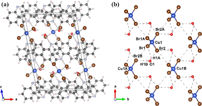
We use coordination chemistry to generate a tuneable family of low-dimensional materials in which $S=1/2$ Cu²⁺ ions are linked magnetically via a superexchange pathway mediated by halide bonds. Previous work shows that by substituting halide ions in the superexchange pathway, differing exchange strengths can be realised Schlueter ; Liu ; thede . The square lattice case is addressed here through pulsed-field magnetization and muon-spin relaxation ($\mu^{+}$SR) measurements of the series (QuinH)₂Cu(Cl_xBr_1-x)${}_{4}\cdot$2H₂O (QuinH=Quinolinium, C₉H₈N⁺) lynch ; Butcher ; landee_new ; si . This combination of techniques is well suited to determining the magnetic ground state of low-dimensional Cu²⁺ complexes Goddard ; Goddard2016 ; landee . Our series is based on 2D antiferromagnetic (AF) layers of Cu$Z_{4}^{2-}$ distorted tetrahedra (where the halide $Z$ = Cl or Br). Tetrahedra are related by C-centering, resulting in a square magnetic lattice, with each $S=1/2$ Cu²⁺ ion having four identical nearest neighbours. Hydrogen bonding to water molecules within the layer generates close $Z$–$Z$ contacts, providing the AF superexchange pathway [Fig. 1(b)]. These 2D AF layers are well isolated owing to the presence of alternating layers of QuinH cations [Fig 1(a)]. The magnetic properties of the $x=0$ compound (QuinH)₂CuBr${}_{4}\cdot$2H₂O suggest it represents a good realization of the 2D QHAF model with intraplane exchange strength $J(x=0)=6.17(3)$ K Butcher . Comparing $x=1$ ($Z$ = Cl) and $x=0$ ($Z$ = Br) materials, there are differences of only 4$\%$ and 0.4$\%$ respectively in the distance between Cu²⁺ ions along the $a$-axis and $b$-axis. However, the change in the interaction strength caused by the varying chemical composition of the superexchange pathways will have a much larger effect than these small differences would suggest. Energy-dispersive X-ray spectroscopy (EDX) measurements si were used to determine $x$ and confirm that there is no macroscopic separation of Br- and Cl-rich structures.

II Results

II.1 Magnetometry

To determine the effective intraplane exchange $J$, low-temperature ($T\approx 0.6$ K) pulsed-field magnetization measurements were made on materials with $0\leq x\leq 1$ (Fig. 2) (see also the Supplemental Material si where the full data set is presented along with further details of the analysis). Magnetization measurements are made at $T\ll J$ where collective behaviour of the spins is expected. The magnetization $M$ as a function of applied field for the $x=0$ and 1 materials [Fig. 2(a)] shows a convex rise to saturation, indicative of 2D magnetic interactions Goddard . Where sufficient correlations (promoted by a narrow distribution in $J$) are present (see below), saturation of $M$ at applied field $H_{\mathrm{sat}}$ occurs via a sharp change in the slope of $M$, giving rise to a minimum in d${}^{2}M/$d$H^{2}$ that allows $H_{\mathrm{sat}}$ to be determined. For $x=0$, this occurs at $\mu_{0}H_{\mathrm{sat}}=16.9(4)$ T, whereas for $x=1$ we find $\mu_{0}H_{\mathrm{sat}}=3.8(3)$ T [Fig. 2(b) and (c)]. The Hamiltonian that describes the two end members of the family is

$${\cal H}=J\sum_{\langle i,j\rangle_{\parallel}}{\bf S}_{i}\cdot{\bf S}_{j}+J_{\perp}\sum_{\langle i,j\rangle_{\perp}}{\bf S}_{i}\cdot{\bf S}_{j}-g\mu_{\rm B}B\sum_{i}S_{i}^{z},$$ (1)

where $J$ is the strength of the exchange coupling within the magnetic planes, $J_{\perp}$ is the coupling between planes, and $J\gg J_{\perp}$. The first two terms on the right hand side refer to summations over unique exchange bonds parallel and perpendicular to the planes, respectively. For $S=1/2$ spins, within a mean-field treatment of this modelGoddard , saturation occurs when $g\mu_{\textsc{B}}\mu_{0}H_{\mathrm{sat}}=zJ$ and $z=4$ is the number of nearest neighbours in the 2D planes. Using the published value of $g=2.15$ for the $x=0$ material Butcher , this gives $J(x=0)=6.1(1)$ K, in good agreement with the previous estimate. Assuming a similar $g$-factor, a value of $J(x=1)=1.4(1)$ K is obtained, in good agreement with the value derived from susceptibility measurementslandee_new and consistent with previous measurements that suggest $J_{\textrm{Br}}\approx 4J_{\textrm{Cl}}$ for Cu²⁺ QHAFs Schlueter .

Figure 2: Low-temperature ($T\approx 0.6$ K) single-crystal magnetization data for (QuinH)₂Cu(Cl_xBr_1-x)₄. (a)-(c) M(H), d$M/$d$H$ and d${}^{2}M/$d$H^{2}$ for $x=0$ and $x=1$. (d) Low and high values of $x$ show a sharp feature in $M(H)$ at $H_{\textrm{sat}}$, but (e) intermediate values do not. Data for (f) $x=0.41$, (g) $x=0.57$, (h) $x=0.605$ and (i) $x=0.74$ showing the smooth approach to saturation in the intermediate values of $x$. Black arrows indicate $H_{\textrm{sat}}$, horizontal black dashed lines correspond to zero values of the derivatives, and orange arrows indicates the low- field kink feature discussed in the text. Data for all samples are provided in the Supplemental Material (si, ).

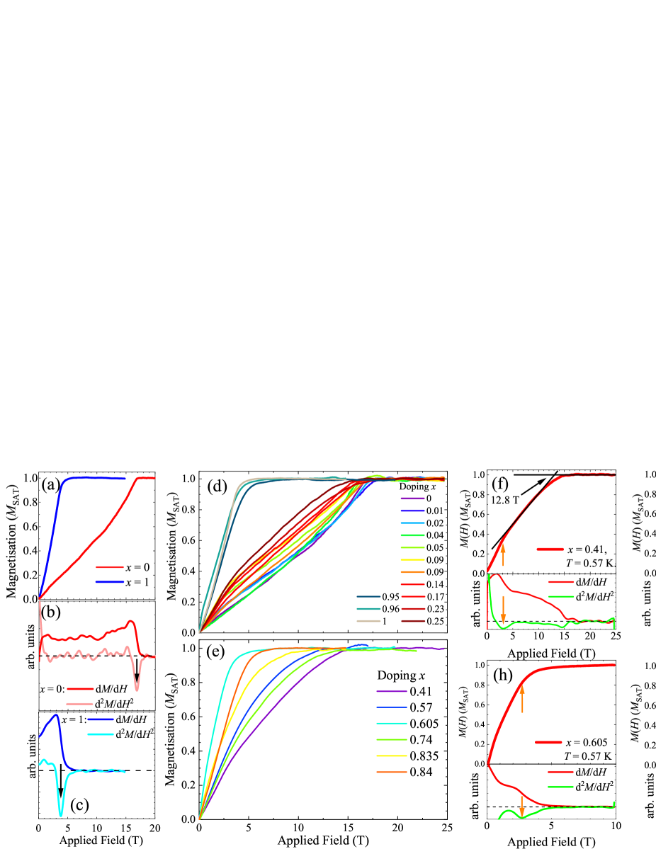
For concentrations with $x\gtrsim 0$ we again measure the characteristic 2D convex rise to saturation, but this becomes less pronounced for $x\geq 0.05$ where the saturation field [and therefore $J(x)$] decreases and the change in the slope of $M(H)$ becomes less sharp [Fig. 2 (d)]. As $x$ is increased further towards $x\approx 0.4$, the approach to saturation broadens, such that the trough in d${}^{2}M/$d$H^{2}$ is hard to discern si . However, a sharp elbow in $M(H)$ is still observed at the saturation field, which can be identified by extrapolation of the data above and below $H_{\mathrm{sat}}$ [Fig. 2(f)]. For $x=0.57,0.74$ and $0.835$ there is no clear feature in the $M(H)$ data si and it is not possible to estimate an effective value for $J$ [Fig. 2(e) and (g–i)]. In this region $M(H)$ no longer exhibits its convex form, but instead rises smoothly with decreasing gradient up to saturation. This behaviour is reminiscent of a disordered system, however the data cannot be fitted to a fully paramagnetic model. This suggests that, while interactions between spins exist, correlations characterized by a single effective exchange energy are not present, or drop below a certain critical length scale. The sharp change in the slope of $M(H)$ at saturation becomes resolvable again for $x\geq 0.84$ and, as the concentration approaches $x=1$, the traces develop the convex shape observed at low $x$. This is consistent with the return to 2D QHAF behavior in the $x=1$ material.

We can assess the coherence length $\xi$ required to give a resolvable transition in $M(H)$ through temperature-dependent pulsed-field measurements of the $x=0$ compound between 0.5 and 15 K, shown in the Supplemental Material si . As $T$ is raised, the saturation point becomes more rounded such that the width of the trough in d${}^{2}M/$d$H^{2}$ increases and the amplitude decreases. For $T\gtrsim 4$ K it is no longer possible to clearly identify $H_{\mathrm{sat}}$. The coherence length in square lattice planes can be estimated using $\xi/d\approx 0.498(1–0.44T/J)$exp$(1.131J/T)$ where $d$ is the magnetic lattice parameter twelve , which holds for $H=0$ and $T\ll J$. Coupling this formula with the limiting value of $T$, above which $H_{\mathrm{sat}}$ is undefined, suggests that the magnitude of exchange can be identified only when $\xi/d\gtrsim 2$ at $H=0$.

In addition to the feature at saturation, the $M(H)$ data for some samples show a kink at fields considerably lower than $H_{\rm sat}$ for the $x=1$ system. The kink is resolvable for several $x$ between 0.05 and 0.61, indicated by an orange arrow in Figs. 2(f) and (h). We attribute this to the presence of isolated clusters of spins (e.g. dimers, trimers, square plaquettes, etc.) coupled by Cl–Cl halide exchange bonds, which are weaker than Br–Br bonds and thus easier to saturate with an applied field. (The effect of these localized units is discussed below.)

II.2 Muon-spin relaxation

Figure 3: Results of ZF $\mu^{+}$SR measurements. (a-f) Top: Example high-temperature spectra; Middle: example low-temperature spectra; Bottom: Example oscillation frequency $\nu$, relaxation rate $\lambda$ or stretching parameter $\delta$ from the function ${\rm e}^{-(\lambda t)^{\delta}}$ (see main text).

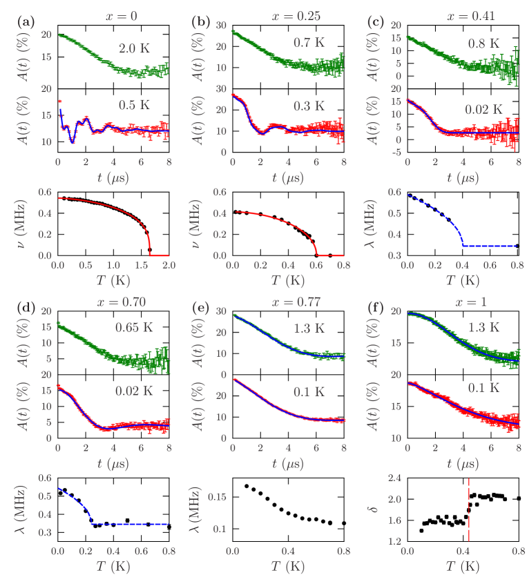
Although the ideal 2D QHAF should only show long-range magnetic order (LRO) at $T=0$, in any realization of the model in a three-dimensional material the presence of interplane exchange $J_{\perp}$ can lead to a transition with $T_{\mathrm{N}}>0$. To determine $T_{\mathrm{N}}$, zero-field (ZF) $\mu^{+}$SR measurements were made steve ; yaouanc . Oscillations in the asymmetry are observed in some members of the series at low $T$ (Fig. 3), providing unambiguous evidence of LRO. For materials with $x\leq 0.25$ oscillations are observed at multiple ($n=2$ or $n=3$) frequencies $\nu_{i}$ [Fig. 3(a,b)] consistent with several magnetically inequivalent muon sites. The oscillatory spectra can be fitted to a function of the form

$$A(t)=\sum_{i=1}^{n}A_{i}e^{-\lambda_{i}t}\cos(2\pi\nu_{i}t+\phi_{i})+A_{\mathrm{bg}}e^{-\lambda_{\mathrm{bg}}t}.$$ (2)

where the last term accounts for muons with their initial spin polarization along the direction of the local magnetic field, along with those muons that stop in the sample holder. The frequencies were held in fixed proportion for the fits (fitting parameters are given in the Supplemental Material si ) From the behaviour of the oscillatory frequency versus temperature, the ordering temperature $T_{\mathrm{N}}$ for each of the compounds can be extracted using the function $\nu_{i}(T)=\nu_{i}(0)\left[1-\left(T/T_{\mathrm{N}}\right)^{\alpha}\right]^{\beta}$, which provides values consistent with discontinuous changes in amplitude that also occur at the ordering transition. We find $T_{\mathrm{N}}(x=0)=1.65(1)$ K, and transition temperatures that decrease smoothly with increasing $x$, such that $T_{\mathrm{N}}(x)$ extrapolates to zero at $x\approx 0.35$. The frequencies $\nu_{i}(T\rightarrow 0)$ are proportional to the moment size on the Cu²⁺ ions and hence to the sublattice magnetization $m$. We measure relatively small frequencies compared to typical 3D systems, reflecting a reduced ordered moment (expected to be 0.33$\mu_{\mathrm{B}}$ for $T\rightarrow 0$ in spin wave theory manou ). These frequencies decrease with increasing $x$ with $m$ dropping by around 24% from $x=0$ to $0.25$.

The behavior is qualitatively different for samples with $0.41\leq x\leq 0.77$ [Fig. 3(c–e)] where no oscillations are resolved down to 0.02 K. Instead, spectra resemble a distorted Kubo-Toyabe (KT) functionyaouanc at low $T$, corresponding to disordered quasistatic moments in the materials, with the distortion of the spectra likely reflecting short-range order along with some limited dynamic fluctuations. As $T$ is increased, the spectra change such that they resemble dynamic, exponential functions above $T\gtrsim 0.5$ K. These data can be parametrized using a stretched-exponential envelope function $e^{-(\lambda t)^{\delta}}$ that accounts for the early time behaviour of the spectra. The transition between the static and dynamic regimes appears abrupt in the $x=0.70$ sample, taking place at a freezing temperature to a glassy configuration around $T_{\mathrm{f}}=0.27$ K, with a similarly rapid variation in relaxation rate seen in the $x=0.41$ material at low temperature, suggesting $T_{\mathrm{f}}\approx 0.41$ K. No such sharp freezing is seen in the $x=0.77$ sample, where the relaxation rate $\lambda$ drops fairly smoothly with increasing $T$ (with a change in slope around $T=0.4$ K, likely related to the freezing seen for other concentrations).

Figure 4: (a) Muon-spin relaxation data for the $x=0.89$ material below (0.1 K) and above (1.2 K) the ordering temperature $T_{\mathrm{N}}$, with a fit shown to a Bessel function relaxation (blue curve, $T<T_{\mathrm{N}}$) and relaxed Kubo-Toyabe function (red curve $T>T_{\mathrm{N}}$). The extracted frequency is plotted in (b), where the line is a guide to the eye. (c) Data for the $x=1$ material below (0.17 K) $T_{\mathrm{N}}$ and above (1.2 K), with a fit to an oscillatory model for the low-temperature data (blue curve) and relaxed Kubo-Toyabe function (red curve $T>T_{\mathrm{N}}$). The extracted frequency is plotted in (d), where the line is a guide to the eye.

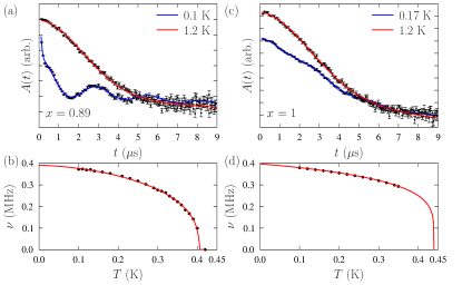
The observed behavior is qualitatively different again in the $x=0.89$ and $x=1$ materials [Fig. 4] where an abrupt transition to LRO takes place with similar $T_{\mathrm{N}}$. Data for the $x=0.89$ material [Fig. 4(a)] can be fitted to a Bessel function, typical of incommensurate magnetic order yaouanc . The presence of incommensurate order might also be consistent with measured data for $0.1\leq x<0.41$ where non-zero phase offsets are observed in the oscillatory components, although the presence of multiple characteristic frequencies complicates the modelling of this feature. The Bessel function results from sampling a distribution of local magnetic fields that varies sinusoidally with position in the material, as expected from an incommensurate spin-density wave. However, depending on the muon sites in a system, there are other field distributions that can lead to relaxation that resembles the Bessel functional form, with its characteristic negative phase shift and damped cosinusoidal temperature dependence. As a result, it is not possible to unambiguously infer the existence of an incommensurate magnetic structure in this composition. In any case, the characteristic frequency decreases smoothly [Fig. 4(b)] allowing $T_{\mathrm{N}}=0.41(1)$ K to be extracted using the same approach as for the materials with $x\leq 0.25$.

Data for the $x=1$ composition show oscillations below the ordering temperature, but at relatively low amplitude compared to other concentrations, as shown in Fig. 4(c). The frequency of these oscillations varies smoothly with temperature [Fig. 4(d)], but cannot be reliably fitted to an oscillatory function close to the transition, where the relaxation rate increases. Such low-amplitude oscillations have been observed previously in similar materials with related structures steele ; lancaster . In this case, the $x=1$ crystallites are notably different in surface colour and form to the other concentrations, and the relatively large ratio of relaxing to oscillatory signal, could reflect the behaviour of muons near the surfaces of these crystallites. However, the transition is via a discontinuous change in the spectra (also seen in the other compositions, where it coincides with the disappearance of the oscillations) and this feature is used to assign $T_{\mathrm{N}}(x=1)=0.44(1)$ K.

For the $x=0$ material, we have $T_{\mathrm{N}}/J=0.27(2)$, which combined with predictions from Quantum Monte Carlo (QMC) simulations 2dformula , suggests $|J_{\perp}/J|\approx 3.2\times 10^{-3}$, indicating well-isolated magnetic layers. At $x=1$ we observe magnetic order with $T_{\mathrm{N}}/J=0.31(2)$ and thus $|J_{\perp}/J|\approx 7.5\times 10^{-3}$. Comparing, we have $J_{\perp}(x=1)=0.014(5)$ K and $J_{\perp}(x=0)=0.011(8)$ K, which is the same within uncertainties, demonstrating that the degree of isolation of the 2D layers is largely unaffected by substitution of Br for Cl ions. This implies that $J_{\perp}(0<x<1)$ is likely close to these values, and that the observed magnetic effects of bond randomness are attributable solely to disorder in the 2D layers.

III Discussion

Figure 5: (a) Fields at which $\mu_{0}H_{\mathrm{sat}}$ (filled symbols) and low-field kink (open symbols) are observed as a function of $x$. (b) Evolution of estimated ordered moment. (c) Notional phase diagram showing antiferromagnetically ordered (AFM), short-range correlated (SRC) and disordered (D) regions. Open triangles show the predicted ordering temperatures from QMC assuming $J_{\perp}=0.011$ K (and no disorder effects aside from a renormalized effective $J$). Dotted line described in main text.

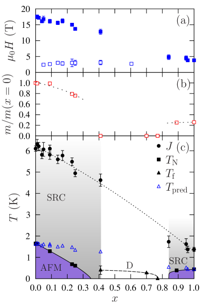
A notional phase diagram for the system is shown in Fig. 5. The parameter $x$ represents the fraction of Cl in a square 2D unit cell with intermediate values corresponding to more exchange-bond disorder. Since halide bonds are formed from two $Z$ ions, the presence of Cl can create a Cl–Cl exchange bond [expected to be around 4 times weaker than Br–Br bond exchange based on the size of $J(x)$] or a mixed Cl–Br bond. The effective exchange strength $J$ extracted from $M(H)$ data provides the energy scale below which we expect short-range AF correlations in 2D planes to dominate the magnetic behaviour for $T_{\mathrm{N}}\ll T\ll J$. The phase diagram is not symmetrical about $x=0.5$ because $x$ does not merely lead to random substitution but also decreases the effective value of $J$ across the series.

We expect the effective exchange $J$ through halide-halide contacts to reflect the size and shape of the orbitals. Structurally, the exchange strength $J$ via the two-halide pathway depends on the identity of the halide ion for two reasons. The first is the shape of the orbitals which leads to better overlap between bromides than between chlorides. The second is that the inter-halide distance is shorter for Cl. By substituting Cl for Br at low levels of doping, the cell constants will still be similar to the $x=0$ compound, so that not only is the Cl ion smaller leading to poor overlap, but the distance between the Cl and Br may be greater than observed in the pure Br material, leading to a still smaller value of $J$. At low concentrations of Br the lattice is similar to the $x=1$ material and the opposite trend might be expected, with Br ions in small spaces causing distortion, and therefore with shorter than expected halide-halide distances, leading to a larger value of $J$.

The extracted values of $J(x)$ [Fig. 5(c)] show a gradual decrease up to $x=0.41$. This is also the region where LRO is observed, with $T_{\mathrm{N}}$ showing a similar gradient to $J(x)$. Combining the measured $J(x)$ with our estimated $J_{\perp}$ we can use the QMC results 2dformula to predict values of $T_{\mathrm{N}}$ assuming disorder leads only to a renormalized effective $J$ (open triangles in Fig. 5). The measured $T_{\mathrm{N}}$ are seen to depart significantly from these predictions, showing that disorder does have a strong effect in suppressing $T_{\mathrm{N}}$ beyond simply the gradual reduction in effective $J$. The ordered moment is seen to decrease as shown in Fig. 5(b). The behaviour in this part of the phase diagram is reminiscent of that for substitutional disorder in La₂Cu_1-z(Zn,Mg)_zO₄ one . A fairly linear decrease was observed in $T_{\mathrm{N}}$ and the ordered moment, along with the disappearance of LRO around $x=0.41$. There is also resemblance to the 1D molecular case in Ref. thede, where $J$ values change approximately linearly across the phase diagram, while $T_{\mathrm{N}}$ and ordered moments drop rapidly on the Br-rich side of the phase diagram. In our case, the energy scales close to $x=1$ are all lower owing to a smaller $J$ mediated by the Cl ions. In the region $0.84\leq x\leq 1$ there is a sufficient correlation length to identify $J$ from the $M(H)$ data and LRO is restored above $x=0.89$. However, $T_{\mathrm{N}}$ close to $x=1$ does not show the rapid decrease seen on the other side of the phase diagram when moving away from the pristine composition, likely because enhanced disorder is also accompanied by an increase in effective $J$.

For $0.41\leq x\leq 0.84$ the magnetic behaviour is more complicated. No LRO can be identified from the $\mu^{+}$SR data across the entire region. The lack of a sharp feature in $M(H)$ at saturation implies that collective behaviour characterized by a single effective exchange $J$ is no longer straightforwardly applicable and that there is therefore a highly magnetically disordered region. Here we see evidence from $\mu^{+}$SR for slow fluctuations of spins for $T\gtrsim 0.5$ K with these becoming more static at the lowest measured temperature, although still not long-range ordered down to 0.02 K. The lack of muon oscillations in the static regime pointsyaouanc to a coherence length $\xi/d\ll 10$. Non-zero $M$ at small applied field implies that this disordered phase is not characterized by an energy gap. For samples with $0.41\leq x\leq 0.7$ there is also evidence for freezing of spins at low $T$. This would appear to suggest freezing of glassy behaviour in this region, as might be expected for a system forming clusters of strongly interacting spins surrounded by disordered moments binder , and seems to be distinct from the spin-liquid-like state predicted for random interactions sandvik2 .

Figure 6: Lower ($x_{c1}$, black solid line) and upper ($x_{c2}$, red solid line) critical substitution levels calculated from the bond-energetics criterion for magnetic-order collapse detailed in the main text as a function of the ratio $J_{\text{Br--Cl}}/J_{\text{Br--Br}}$. (The equations determining these substitution levels are identical when $J_{\text{Br--Cl}}$ vanishes, resulting in a single critical value.) The measured ratio $J_{\text{Cl--Cl}}/J_{\text{Br--Br}}=0.206(15)$ is assumed. Experimentally-observed critical substitution levels $x_{c1}$ and $x_{c2}$ are indicated by horizontal dashed lines with one-sigma shaded regions around them. The green shaded region highlights the range of ratios $J_{\text{Br--Cl}}/J_{\text{Br--Br}}$ compatible with $x_{\mathrm{c}1}$ and $x_{\mathrm{c}2}$ within one sigma. The simple guess $J_{\text{Br--Cl}}/J_{\text{Br--Br}}\approx\sqrt{J_{\text{Cl--Cl}}/J_{\text{Br--Br}}}$ is shown as a grey vertical dashed line and lies outside the experimentally-allowed green region, while the actual value of $J_{\text{Br--Cl}}/J_{\text{Br--Br}}$ extracted from the best fit of the average exchange $J(x)$ [dashed line in Fig. 5(c)] is shown by a blue vertical line and is compatible with experimental $x_{\mathrm{c}1}$ and $x_{\mathrm{c}2}$. One-sigma uncertainty intervals for both of these values are shown by horizontal error bars on the bottom axis.

We consider here three potential effects driving the form of the phase diagram: (i) percolation; (ii) bond energetics and (iii) quantum fluctuations. The bond percolation threshold for a square lattice is stauffer $p_{\mathrm{c}}=1/2$. However, for our materials a single exchange bond comprises two possible substitution sites. If a single substitution per bond suffices to destabilize magnetic order then we should equate the percolation threshold $p_{\mathrm{c}}$ to the probability that one or more substitutions occurs on a single exchange bond $p_{\mathrm{c}}=1-(1-x_{\mathrm{c}1})^{2}$, which gives a lower critical substitution level $x_{\mathrm{c}1}=0.29$, while at high $x$, we should have $p_{\mathrm{c}}=1-x_{\mathrm{c}2}^{2}$, which gives an upper critical substitution level $x_{\mathrm{c}2}=1-x_{\mathrm{c}1}=0.71$. This could be compatible with the data for $x<0.41$, but fails to describe the large-$x$ behavior. Furthermore, it is unlikely that percolation is the sole driver of the observed behaviour since we are changing the strengths of random bonds, rather than removing exchange pathways. More sophisticated correlated percolation models including lattice-dependent grouping of substituted bonds also fail to describe the measured phase diagram. The possibility of such clusters forming, their size and the effect of correlated substitutions are discussed in Appendix A.

An approximate criterion for the collapse of magnetic order (which could be short range) might be when the total exchange energy of substituted bonds becomes larger than that of unsubstituted bonds. We would expect a lower critical substitution level $x=x_{\mathrm{c}1}$ to be determined by Br–Cl and Cl–Cl bonds acting as disorder in a Br–Br ordered background such that $(1-x_{\mathrm{c}1})^{2}J_{\mathrm{Br}-\mathrm{Br}}=2x_{\mathrm{c}1}(1-x_{\mathrm{c}1})J_{\mathrm{Br}-\mathrm{Cl}}+x_{\mathrm{c}1}^{2}J_{\mathrm{Cl}-\mathrm{Cl}}$. The upper critical substitution level $x=x_{\mathrm{c}2}$ is then determined by Br–Cl and Br–Br bonds acting as disorder in a Cl–Cl ordered background giving $x_{\mathrm{c}2}^{2}J_{\mathrm{Cl}-\mathrm{Cl}}=2x_{\mathrm{c}2}(1-x_{\mathrm{c}2})J_{\mathrm{Br}-\mathrm{Cl}}+(1-x_{\mathrm{c}2})^{2}J_{\mathrm{Br}-\mathrm{Br}}$. The unknown exchange strength in these expressions, $J_{\text{Br--Cl}}$, can be determined by fitting the measured $J(x)$ with $J(x)=(1-x)^{2}J_{\text{Br--Br}}+2x(1-x)J_{\text{Br--Cl}}+x^{2}J_{\text{Cl--Cl}}$, which describes the data well [dotted line, Fig. 5(c)] and gives estimates $J_{\text{Br--Br}}=6.2(1)~{}\mathrm{K}$, $J_{\text{Br--Cl}}=4.3(3)~{}\mathrm{K}$, and $J_{\text{Cl--Cl}}=1.3(1)~{}\mathrm{K}$. These yield the critical substitution levels $x_{\mathrm{c1}}=0.40(2)$ and $x_{\mathrm{c2}}=0.88(2)$, both of which agree well with the observed location of the collapse of magnetic order.

In fact, values of $x_{\mathrm{c}}$ compatible with experiment result from only a limited range of choices for the ratio $J_{\text{Br--Cl}}/J_{\text{Br--Br}}$. We can express the expected lower and upper critical substitution levels $x_{c1}$ and $x_{c2}$, respectively, as a function of the two exchange-strength ratios $J_{\text{Br--Cl}}/J_{\text{Br--Br}}$ and $J_{\text{Cl--Cl}}/J_{\text{Br--Br}}$. Fixing the known pristine-system exchange-strength ratio $J_{\text{Cl--Cl}}/J_{\text{Br--Br}}=0.206(15)$, the observed critical substitution levels $x_{c1}=0.32(9)$ and $x_{c2}=0.83(6)$ put stringent limits on the range of experimentally allowed ratios $J_{\text{Br--Cl}}/J_{\text{Br--Br}}=0.65\text{--}0.78$ (Fig. 6). This is incompatible with the most simple assumption that each substitution of a Br with a Cl ion weakens the exchange bond (which consists of two Br/Cl sites) by the same factor, which would yield $J_{\text{Br--Cl}}/J_{\text{Br--Br}}\approx\sqrt{J_{\text{Cl--Cl}}/J_{\text{Br--Br}}}=0.45(2)$. On the other hand, the enhanced ratio $J_{\text{Br--Cl}}/J_{\text{Br--Br}}=0.69(5)$ extracted from the best fit of the average exchange model to the measured $J(x)$ [Fig. 5(c)] is fully compatible with the observed critical substitution levels via the bond-energetics criterion (Fig. 6). This validates both the bond-energetics criterion for the collapse of magnetic order in the 2D square-lattice QHAF as well as the average-exchange $J(x)$ model described above.

Finally, theory predicts that the disorder-driven introduction of antiferromagnetically-coupled dimers, chains or other clusters acts to enhance quantum fluctuations, destroying long-range magnetic order three ; sandvik2 . This scenario is consistent with our observations: the presence of the low-field kink in our magnetometry data points to high densities of microscopic clusters of Cu moments coupled by Cl bonds, while our EDX measurements showed no evidence for phase separation, suggesting inhomogeneities are limited to a local level. Calculations indeed show (Appendix A) that a random distribution of disordered bonds leads to a large concentration of dimers and trimers around $x=0.2$, where we see $T_{\mathrm{N}}$ being strongly suppressed towards disorder.

IV Conclusion

In summary, the addition of small amounts of disorder to the pristine 2D QHAF causes regions of the sample to remain correlated with a single effective $J$, which decreases as $x$ increases. Simultaneously there is a preponderance for formation of minority clusters (e.g. dimers and trimers) that enhance quantum fluctuations and act to suppress $T_{\rm N}$ more than is predicted from the change in $J$ alone. For $0.41\leq x\leq 0.84$, while spins continue to interact, the correlated regions are no longer apparent, LRO is completely absent and low-temperature spin freezing is evident. Critical substitution levels can be explained by an energetics-based competition between different local magnetic orders. Our result that magnetic order can be destroyed by quantum effects of exchange randomness could have implications for other disordered Q2D AFM systems such as the parent state of the cuprate superconductors, or frustrated square lattices, which are believed to evolve into a spin-liquid state on the introduction of quenched disorder.

Appendix A Calculating the effect of halide substitution on spin clusters

In the main text we described the influence of percolation as a possible driver of the phase diagram of this system. The complication of exchange bonds comprising two possible substitution sites makes this problem more complex than that of a bond being formed from a single substitution sites. We discuss the details of the effects of halide substitutions on spin clusters in this Appendix.

A.1 Formation of spin clusters

Figure 7: A schematic diagram showing a simulation of the two-dimensional lattice in (QuinH)₂Cu(Cl_xBr_1-x)${}_{4}\cdot 2$H₂O for different values of $x$. The coloring of the bonds is black for Br–Br, yellow for Br–Cl, red for Cl–Cl.

Increasing $x$ in (QuinH)₂Cu(Cl_xBr_1-x)${}_{4}\cdot 2$H₂O has the result of replacing Br linkages with Cl linkages in superexchange pathways. Since bonds are formed with two halide ions, the connections between magnetic Cu²⁺ ions change from being all Br–Br links at $x=0$ (colored black in Fig. 7) to all Cl–Cl links at $x=1$ (colored red). However, at intermediate $x$ there are many Br–Cl links (colored yellow). This is shown schematically in Fig. 7 in which the bonds are chosen randomly according to the value of $x$ indicated on the vertical axis. This figure illustrates that intermediate values of $x$ give a range of mixtures of different linkages which, as explained in the main text, have different exchange strengths.

Figure 8: The probability of isolated clusters of Cl-containing bonds [dimers (blue), trimers (red) or tetramers (green), corresponding to $s=1$, $2$ and $3$ bond clusters] surrounded by only Br–Br bonds. The dotted line tangent to the $s=1$ curve is described in the text. The percolation threshold for impurity bonds with at least one substitution $x_{\rm c}$ is indicated by the short vertical dotted line. The dashed curves show the effect of including $\pm 30$% additional inhomogeneous clustering of Br- or Cl-rich regions.

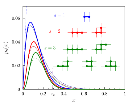
Another way of looking at this problem is shown in Fig. 8 which plots the probability of finding an isolated dimer, trimer or tetramer of spins connected by Cl-containing bonds (either Br–Cl or Cl–Cl) and surrounded by only Br–Br bonds that dominate at low $x$. The probability that a randomly chosen bond contains at least one Cl is $1-(1-x)^{2}=x(2-x)$. Furthermore, we denote by $p_{s}(x)$ the probability that a randomly chosen bond is part of an isolated cluster of Cl-containing bonds of size $s$ (so a spin dimer has $s=1$ because it represents two Cu²⁺ spins connected by a single Cl-containing bond, a spin trimer has $s=2$ because it involves two Cl-containing bonds, etc.). These probabilities are given by $p_{1}(x)=x(2-x)(1-x)^{12}$ for spin dimers [the power of 12 reflecting the six double-bromide bonds that must be present at the boundary of a dimer, a double Br bond having probability $(1-x)^{2}$], $p_{2}(x)=6x^{2}(2-x)^{2}(1-x)^{16}$ for spin trimers (both straight and bent, involving eight double-bromide bonds at the boundary) and $p_{3}=3x^{3}(2-x)^{3}(1-x)^{18}(9(1-x)^{2}+2)$ for tetramers (where various shapes are possible, as shown in Fig. 8). For very small $x$ these values depend mostly on the probability of finding enough Cl-containing bonds (so for dimers, this factor is $1-(1-x)^{2}=x(2-x)$, the dotted blue line in Fig. 8) but this becomes reduced at higher $x$ due to the probability of finding pure Br–Br bonds surrounding the cluster falling substantially below unity. The result is that these isolated species are only reasonably probable below the ideal percolation threshold for impurity bonds with at least one Cl substitution, which is $x=x_{\rm c}=1-1/\sqrt{2}\approx 0.29$ [a value obtainedstauffer from the exact bond percolation threshold for a square lattice in terms of the single bond occupation probability $p_{\mathrm{c}}=1/2=x_{\mathrm{c}}(2-x_{\mathrm{c}})$ ]. Beyond this value clusters start to link up, and these species are practically absent above $x\approx 0.4$. This concentration is roughly consistent with the lower value of $x=x_{\mathrm{c}1}$ at which both the AFM and SRC phases collapse, although this likely reflects the fact that $x\approx 0.4$ lies well above the percolation threshold. This is explored in more detail below.

A.2 Size of spin clusters

The effect of $x$ on these isolated clusters is seen even more clearly in Fig. 9(a) which shows the form of $p_{s}(x)$ as a function of both $x$ and cluster size $s$. These probabilities were computed numerically on the line graph (i.e. graph of bonds) of an $L\times L$ patch of a square lattice with $L=4001$. An $O(L)$ space-complexity algorithm inspired by the modified Hoshen–Kopelman algorithm hoshen1976percolation ; tiggemann2006percolation and generalized to arbitrary lattices was used for this, as described in Ref. gomilsek2019kondo, . Note that $\sum_{s=1}^{\infty}p_{s}(x)=x(2-x)$, the probability that one or more substitutions occurs on a single bond, since the sum over $s$ of probabilities that a randomly chosen bond is a member of a cluster of size $s$ necessarily accounts for all substituted bonds (at least below the percolation threshold). We note that the probabilities of Br-rich bond clusters in a Cl–Cl bond background (which dominate for $x$ near 1) are the same as the ones presented on Figs. 8 and 9 under the duality $x\rightarrow 1-x$ that exchanges the roles of Br and Cl.

Figure 9: (a) A density plot of the cluster probabilities $p_{s}(x)$. (b) The mean size $S$ of bond clusters as a function of $x$. The percolation threshold $x_{\mathrm{c}}$ for impurity bonds with at least one substitution is indicated by a vertical dashed line.

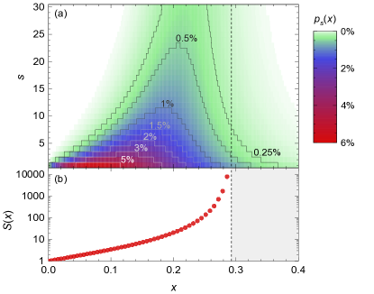
Dividing $p_{s}(x)$ by $x(2-x)$ gives the conditional probability that a randomly-chosen Cl-substituted bond is part of a cluster of size $s$ and allows us to estimate the mean cluster size $S(x)$. This quantity is therefore defined asstauffer $S(x)=\sum_{s=1}^{\infty}sp_{s}(x)/[x(2-x)]$ and answers the question: given a randomly chosen bond with one or more substitutions, what is the mean size of the cluster that this bond is a part of? This is plotted in Fig. 9(b), showing that the mean cluster size increases rapidly as $x$ increases, and diverges as $x\to x_{\rm c}$. Given the sharpness of this percolation transition we conclude that uncorrelated percolation on its own is likely not the sole driver behind the collapse of AFM and SRC order in the material studied in this paper. Namely, the lower critical concentration $x_{c1}=0.40(2)$ is not close enough to the sharp percolation threshold of Cl-rich bond clusters, which occurs at a substantially lower $x_{\mathrm{c}}=1-1/\sqrt{2}\approx 0.29$. The discrepancy is even more acute for the upper critical concentration $x_{\mathrm{c}2}=0.88(2)$, which is substantially higher than the predicted percolation threshold of Br-rich bond clusters $1-x_{\mathrm{c}}=1/\sqrt{2}\approx 0.71$ under the Cl–Br duality. Uncorrelated percolation thus cannot explain the observed critical concentrations for the collapse of AFM and SRC order in these systems.

A.3 Effect of correlated substitutions

Going beyond uncorrelated percolation, we first consider the effect of locally-correlated substitution on individual bonds due to structural consequences of changing the size of the halide ion (the ionic radius of Br^- is ${\approx}~{}8\%$ larger than that of Cl^-). Denoting the probabilities that a randomly chosen bond is a Br–Br bond, a Cl–Cl bond or a mixed Br–Cl bond, by $p_{\text{Br--Br}}$, $p_{\text{Cl--Cl}}$ and $p_{\text{Br--Cl}}$, respectively, uncorrelated substitutions of Br by Cl on bonds would correspond to the probabilities: $p_{\text{Br--Br}}^{0}=(1-x)^{2}$, $p_{\text{Br--Cl}}^{0}=2x(1-x)$ and $p_{\text{Cl--Cl}}^{0}=x^{2}$ (where the superscript $0$ labels the probability for an uncorrelated substitution). Structural changes might skew these probabilities, but they must obey $p_{\text{Br--Br}}+p_{\text{Br--Cl}}+p_{\text{Cl--Cl}}=1$, and reproduce the observed Cl concentration by obeying $p_{\text{Br--Cl}}/2+p_{\text{Cl--Cl}}=x$. Denoting the $x$-dependent probability difference ${\Delta p}(x)=p_{\text{Br--Cl}}(x)-p_{\text{Br--Cl}}^{0}(x)$ for finding a mixed Br–Cl bond, so that ${\Delta p}=0$ would correspond to locally-uncorrelated substitutions, we get: $p_{\text{Br--Br}}=(1-x)^{2}-{\Delta p}/2$, $p_{\text{Br--Cl}}=2x(1-x)+{\Delta p}$ and $p_{\text{Cl--Cl}}=x^{2}-{\Delta p}/2$. In this model the lower percolation threshold of Cl-rich bond clusters would correspond to the condition: $1-p_{\text{Br--Br}}(x_{\mathrm{c}1})=p_{\mathrm{c}}=1/2$, while the upper percolation threshold for Br-rich bond clusters would correspond to the condition: $1-p_{\text{Cl--Cl}}(x_{\mathrm{c}2})=p_{\mathrm{c}}=1/2$. Solving for the mixed-bond probability shift ${\Delta p}$ assuming locally-correlated bond substitutions we get ${\Delta p}(x_{\mathrm{c}1})=-0.28(5)$ and ${\Delta p}(x_{\mathrm{c}2})=+0.55(7)$, which correspond to a decrease of mixed-bond probabilities by $-58(7)\%$ at $x=x_{\mathrm{c}1}$ and an increase of mixed-bond probabilities by $+260(80)\%$ at $x=x_{\mathrm{c}2}$. The huge shifts in probabilities that this model would require are implausible, allowing us to reject this percolation model with purely bond-local substitutional correlations.

We also tested the effect of including additional clustering effects between different neighbouring bonds (i.e. a scenario of inter-bond correlated percolation) due to the structural consequences of changing the size of the halide ion. This could mean that slightly Br-rich regions and slightly Cl-rich regions could spontaneously form in a crystal prepared with a particular nominal $x$, though we stress that we have no experimental evidence that this effect occurs in our samples. To model this, we considered a sample with an equal mixture of regions with $x(1+\epsilon)$ and with $x(1-\epsilon)$ and illustrate the effect in Fig. 8 for $\epsilon=0.3$. This would be an extremely high level of clustering, but the simulations show that this does not alter the general conclusions stated above. The only effect observed is a small shift of the probability of isolated dimers, trimers and tetramers to larger values of $x$ (due, of course, to regions of the sample in which $x$ is smaller than the nominal value). We conclude that our picture of isolated clusters of Cl-rich bonds growing as $x$ increases, starting to coalesce and essentially disappearing completely above around $x\approx 0.4$ is fairly robust to clustering effects and cannot explain the conflicting experimental values of $x_{\mathrm{c}1}>x_{\mathrm{c}}$ and $x_{\mathrm{c}2}\gg 1-x_{\mathrm{c}}$.

For a quantitative understanding of correlation effects we consider the exact correlated-percolation model of Ref. gomilsek2019kondo, , where a shift of probability that a bond is substituted by Cl if a neighbouring bond is also substituted by Cl by some constant factor $\gamma>0$, where $\gamma=1$ corresponds to uncorrelated percolation, would correspond to an effective rescalinggomilsek2019kondo $p\rightarrow\mathrm{min}(\gamma p_{0},1)$ of the probability that a bond contains at least one Cl, where $p_{0}=x(2-x)$ is the uncorrelated probability. Since the lower experimental critical concentration $x_{\mathrm{c}1}$ is larger than the uncorrelated percolation expectation of $x_{\mathrm{c}}=1-1/\sqrt{2}\approx 0.29$, we would get $\gamma=p_{\mathrm{c}}/p_{0}(x_{\mathrm{c}1})=0.78(3)<1$. This is quite a large deviation from uncorrelated percolation (it corresponds to a Pearson correlation coefficient of $\phi=(\gamma-1)/(p^{-1}_{\mathrm{c}}-1)=-0.22(3)$ at the percolation threshold), and being less than unity means that nearby Cl-substituted bonds are less likely than expected for uncorrelated Cl substitutions. The effect would be that Cl would actually be dispersed more evenly throughout the sample than by pure uncorrelated chance. By extension, in the dual view of rare Br bond substitutions in a Cl–Cl bond background (valid for $x\approx 1$) one should also get less clustering of Br-rich bonds (as clustering of Br-rich bonds would also push Cl-rich bonds closer together, rather than further apart as required by $\gamma<1$), meaning that the dual upper critical concentration $x_{\mathrm{c}2}$ should get pushed to lower values (further away from $x=1$) than the uncorrelated expectation of $1-x_{\mathrm{c}}=1/\sqrt{2}\approx 0.71$, in clear contradiction with experiment where $x_{\mathrm{c}2}=0.88(2)\gg 0.71$.

We therefore conclude that a dual pair of pure percolation transitions of Cl- and Br-rich bond clusters cannot explain the experimentally observed critical concentrations $x_{\mathrm{c}1}$ and $x_{\mathrm{c}2}$ neither via uncorrelated Cl substitutions, via bond-local correlation of Cl substitutions, nor via inter-bond substitutional correlation effect gomilsek2019kondo . In contrast, the experimentally observed critical concentrations are reproduced relatively straightforwardly using a simple position-blind model of substituted-bond energetics (see previous section). We therefore conclude that a lattice-dependent bias towards grouping of substituted bonds must not be particularly significant in the system that we have studied, and is therefore not the primary driver behind the ultimate collapse of AFM and SRC order, which most likely originates from an energetics-based competition between different local magnetic orders. On the other hand, the simple unbiased model confirms the random formation of minority clusters (e.g. dimers and trimers) at low substitution values, as suggested by the magnetisation measurements. We reassert that these clusters will promote quantum fluctuations, and in all likelihood account for the observed suppression of $T_{\mathrm{N}}$ beyond that which would be expected from the reduction in the effective exchange strength alone.

References

- (1) M. Urai, K. Miyagawa, T. Sasaki, H. Taniguchi, and K. Kanoda, Phys. Rev. Lett. 124, 117204 (2020).
- (2) K. W. Plumb, Hitesh J. Changlani, A. Scheie, S. Zhang, J. W. Krizan, J. A. Rodriguez-Rivera, Yiming Qiu, B. Winn, R. J. Cava and C. L. Broholm, Nature Physics 15, 54 (2019).
- (3) I. Kimchi, J.P. Sheckelton, T.M. McQueen and P.A. Lee Nature Communications 9, 4367 (2018).
- (4) O. Mustonen, S. Vasala, E. Sadrollahi, K. P. Schmidt, C. Baines, H. C. Walker, I. Terasaki, F. J. Litterst, E. Baggio-Saitovitch and M. Karppinen, Nature Communications 9, 1085 (2018),
- (5) L. Savary and L. Balents, Phys. Rev. Lett. 118, 087203 (2017)
- (6) A.W. Sandvik, Phys. Rev. B 66, 024418 (2002).
- (7) N. Laflorencie, S. Wessel, A. Läuchli, and H. Rieger, Phys. Rev. B 73, 060403(R) (2006).
- (8) R. Yu, T. Roscilde and S. Haas, Phys. Rev. B 73, 064406 (2006).
- (9) L. Liu, H. Shao, Y.-C. Lin, W. Guo,and A.W. Sandvik, Phys. Rev. X 8, 041040 (2018).
- (10) S. Liu and A. L. Chernyshev, Phys. Rev. B 87, 064415 (2013).
- (11) The distinction between classical and quantum in this context rests on whether the properties of the system can be described using magnetic moments free to point in any direction, or if the quantization of spin components must be considered.
- (12) O. P. Vajk, P. K. Mang, M. Greven, P. M. Gehring, and J. W. Lynn, Science 295, 1691 (2002).
- (13) V. Wagner and U. Kray, Z. Physik B 30, 367 (1978).
- (14) Y. Okuda, Y. Tohi, I. Yamada and T. Haseda, J. Phys. Soc. Jpn. 49, 936 (1980).
- (15) C. Binek and W. Kleemann, Phys. Rev. B 51, 12888 (1995).
- (16) O. Mustonen, S. Vasala, E. Sadrollahi, K. P. Schmidt, C. Baines, H. C. Walker, I. Terasaki, F. J. Litterst, E. Baggio-Saitovitch and M. Karppinen, Nature Commun. 9, 1085 (2018).
- (17) H. Kawamura and K. Uematsu, J. Phys.: Condens. Matter 31, 50 (2019).
- (18) T. Furukawa, K. Miyagawa, T. Itou, M. Ito, H. Taniguchi, M. Saito, S. Iguchi, T. Sasaki, and K. Kanoda, Phys. Rev. Lett. 115, 077001 (2015).
- (19) J.A. Schlueter, H. Park, G.J. Halder, W.R. Armand, C. Dunmars, K.W. Chapman, J.L. Manson, J. Singleton, R. McDonald, A. Plonczak, J. Kang, C. Lee, M.-H. Whangbo, T. Lancaster, A.J. Steele, I. Franke, J.D. Wright, S.J. Blundell, F.L. Pratt, J. deGeorge, M.M. Turnbull, and C.P. Landee, Inorg. Chem. 51, 2121 (2012).
- (20) J. Liu, P. A. Goddard, J. Singleton, J. Brambleby, F. Foronda, S. J. Blundell, T. Lancaster, F. Xiao, R. C. Williams, F. L. Pratt, P. J. Baker, J. S. Möller, Y. Kohama, S. Ghannadzadeh, A. Ardavan, K. Wierschem, S. H. Lapidus, K. H. Stone, P. W. Stephens, J. Bendix, T. J. Woods, K. E. Carreiro, H. E. Tran, C. J. Villa, and J. L. Manson, Inorg. Chem 55, 3515 (2016).
- (21) M. Thede, F. Xiao, Ch. Baines, C. Landee, E. Morenzoni, and A. Zheludev Phys. Rev. B 86, 180407(R) (2012).
- (22) D.E. Lynch and I McClenaghan, Acta. Crystallogr. E 58, m551 (2002).
- (23) R. T. Butcher, M.M. Turnbull, C.P. Landee, A. Shapiro, F. Xiao, D. Garrett, W.T. Robinson and B. Twamley, Inorg. Chem. 49, 427 (2010).
- (24) C.P. Landee, J.C. Monroe, R. Kotarba, M. Polson, J.L. Wikaira and M.M. Turnbull, J. Coord. Chem. 71, 3342 (2018).
- (25) Supplementary Material contains descriptions of the material preparation, experimental methods and further data on each composition measured.
- (26) P. A. Goddard, J. Singleton, P. Sengupta,, R. D. McDonald, T. Lancaster, S. J. Blundell, F. L. Pratt, S. Cox, N. Harrison, J. L. Manson, H. I. Southerland and J. A. Schlueter, New J. Phys. 10, 083025 (2008).
- (27) P. A. Goddard, J. Singleton, I. Franke, J. S. Moller, T. Lancaster, A. J. Steele, C. V. Topping, S. J. Blundell, F. L. Pratt, C. Baines, J. Bendix, R. D. McDonald, J. Brambleby, M. R. Lees, S. H. Lapidus, P. W. Stephens, B. W. Twamley, M. M. Conner, K. Funk, J. F. Corbey, H. E. Tran, J. A. Schlueter, and J. L. Manson, Phys. Rev. B 93, 094430 (2016).
- (28) F. M. Woodward, A. S. Albrecht, C. M. Wynn, C. P. Landee, and M. M. Turnbull, Phys. Rev. B 65, 144412 (2002)
- (29) P. Hasenfratz and F. Niedermayer, Phys. Lett. B 268, 231 (1991); B. B. Beard, R. J. Birgeneau, M. Greven, and U.-J. Wiese, Phys. Rev. Lett. 80, 1742 (1998); M. A. Kastner, R. J. Birgeneau, G. Shirane, and Y. Endoh, Rev. Mod. Phys. 70, 897 (1998).
- (30) S.J. Blundell, Contemp. Phys. 40, 175 (1999).
- (31) A. Yaouanc and P. Dalmas de Reotier Muon Spin Rotation, Relaxation, and Resonance (Oxford: OUP) (2010).
- (32) A.J. Steele, T. Lancaster, S.J. Blundell, P. J. Baker, F.L. Pratt, C. Baines, M.M. Conner, H.I. Southerland, J.L. Manson, and J.A. Schlueter, Phys. Rev. B 84, 064412 (2011).
- (33) T. Lancaster, S.J. Blundell, F.L Pratt, M.L. Brooks, J.L. Manson, E.K. Brechin, C. Cadiou, D. Low, E.J.L. McInnes and R.E.P Winpenny, J. Phys. Condens. Matter 16, S4563 (2004).
- (34) E. Manousakis, Rev. Mod. Phys. 63, 1 (1991).
- (35) C. Yasuda, S. Todo, K. Hukushima, F. Alet, M. Keller, M. Troyer, and H. Takayama, Phys. Rev. Lett. 94, 217201 (2005).
- (36) K. Binder and A.P. Young, Rev. Mod. Phys. 58, 801 (1986).
- (37) D. Stauffer and A. Aharony Introduction to Percolation Theory (Taylor and Francis, London) (1991).
- (38) J. Hoshen and R. Kopelman, Phys. Rev. B 14, 3438 (1976).
- (39) D. Tiggemann, Int. J. Mod. Phys. C 17, 1141 (2006).
- (40) M. Gomilšek, R. Žitko, M. Klanjšek, M. Pregelj, C. Baines, Y. Li, Q.M. Zhang and A. Zorko, Nature Phys. 15, 754 (2019).