A FAST ALGORITHM FOR THE PRODUCT STRUCTURE OF PLANAR GRAPHS

Abstract

Dujmović et al.  (FOCS2019) recently proved that every planar graph $G$ is a subgraph of $H\boxtimes P$, where $\boxtimes$ denotes the strong graph product, $H$ is a graph of treewidth 8 and $P$ is a path. This result has found numerous applications to linear graph layouts, graph colouring, and graph labelling. The proof given by Dujmović et al.  is based on a similar decomposition of Pilipczuk and Siebertz (SODA2019) which is constructive and leads to an $O(n^{2})$ time algorithm for finding $H$ and the mapping from $V(G)$ onto $V(H\boxtimes P)$. In this note, we show that this algorithm can be made to run in $O(n\log n)$ time.

1 Introduction

The strong product $G_{1}\boxtimes G_{2}$ of two graphs $G_{1}$ and $G_{2}$ is the graph whose vertex set is the Cartesian product $V(G_{1})\times V(G_{2})$ in which the vertices $(v,x)$ and $(w,y)$ are adjacent if and only if

• $v=w$ and $xy\in E(G_{2})$;

• $vw\in E(G_{1})$ and $x=y$; or

• $vw\in E(G_{1})$ and $xy\in E(G_{2})$.

Dujmović et al.  [5] recently proved the following product structure theorem for planar graphs:

Theorem 1 (Dujmović et al. 2019).

For any $n$-vertex planar graph $G$, there exists a graph $H$ of treewidth at most 8 and a path $P$ such that $G$ is a subgraph of $G^{+}:=H\boxtimes P$.

Though still very new, Theorem 1 has been used to solve a number of longstanding open problems on planar graphs:

• Theorem 1 has been used to show that the queue-number of every planar graph is upper bounded by a constant. This solves an open problem of Heath, Leighton, and Rosenberg posed in 1992 [10].

• Theorem 1 has been used to show that the nonrepetitive chromatic number of every planar graph is upper bounded by a constant. This solves an open problem of Alon et al.  [1] posed in 2002.

• Theorem 1 has been used to produce (asymptotically) optimal labelling schemes for planar graphs [6]. This (asympotically) resolves a problem of Kannan, Naor, and Rudich posed in 1988 [11, 12].

• Theorem 1 has been used to make significant improvements on the best-known bounds for $p$-centered colourings of planar graphs [2]. This gives the strongest result thus far on a question motivated by the work of Nešetřil and Ossona de Mendez from 2006 [16, 17] and posed explicity by Dvořák in 2016 [14].

The proof of Theorem 1 given by Dujmović et al.  is based on a similar decomposition of Pilipczuk and Siebertz [18] which is constructive and leads to an $O(n^{2})$ time algorithm for finding $H$ and the mapping from $V(G)$ onto $V(H\boxtimes P)$ [5, Section 10]. Given the number of applications of Theorem 1 (and that more are likely to be found), it is natural to ask if this running-time can be improved. In this paper, we provide a faster algorithmic version of Theorem 1:

Theorem 2.

For any $n$-vertex planar graph $G$, there exists a graph $H$ of treewidth at most 8 and a path $P$ such that $G$ is a subgraph of $G^{+}:=H\boxtimes P$.

Furthermore, there exists an algorithm that, given $G$ as input, runs in $O(n\log n)$ time and produces the graph $H$, the path $P$, and an injective function $\varphi:V(G)\to V(G^{+})$ such that, for each edge $vw\in E(G)$, $\varphi(v)\varphi(w)\in E(G^{+})$.

The remainder of this paper is organized as follows. Section 2 reviews the proof of Theorem 1 and the resulting $O(n^{2})$ time algorithm. Section 3 describes the $O(n\log n)$ time algorithm. Section 4 discusses some of the implications and generalizations of this work.

2 The Original Proof/Algorithm

Throughout this paper we use standard graph theory terminology as used in the textbook by Diestel [3]. Every graph $G$ that we consider is finite, simple, and undirected, and has vertex set denoted by $V(G)$ and edge set denoted by $E(G)$.

Let $T$ be a tree rooted at some node $r$ and, for each node $v$ of $T$, let $P_{T}(v)$ denote the path in $T$ from $v$ to $r$. The $T$-depth of a node $v$ in $T$ is the length of $P_{T}(v)$. A path $P$ in $T$ is a vertical path if no two nodes of $P$ have the same $T$-depth. Every node $w$ in $P_{T}(v)$ is a $T$-ancestor of $v$ and $v$ is a $T$-descendant of every node $w$ in $P_{T}(v)$. Note that $v$ is both a $T$-ancestor and $T$-descendant of itself.

For a graph $G$ and a partition $\mathcal{P}$ of $V(G)$, the quotient graph $G/\mathcal{P}$ is the graph whose vertices $V(G/\mathcal{P})$ are the sets in $\mathcal{P}$ and in which an edge $XY\in E(G/\mathcal{P})$ if and only if there exists $x\in X$ and $y\in Y$ with $xy\in E(G)$. Dujmović et al.  [5] prove Theorem 1 by first adding edges to a planar graph $G_{0}$ to complete it to a triangulation $G$, computing a breadth-first search tree $T$ of $G$ and then applying the following result to $G$ and $T$:

Theorem 3.

For any $n$-vertex triangulation $G$ and any spanning tree $T$ of $G$, there exists a partition $\mathcal{P}$ of $V(G)$ such that each $P\in\mathcal{P}$ induces a vertical path in $T$ and the quotient graph $H:=G/\mathcal{P}$ has treewidth at most $8$.

Deriving Theorem 1 from Theorem 3 is just a matter of checking definitions. The graph $H$ in Theorem 1 is the same graph $H$ in Theorem 3. The path $P$ in Theorem 1 is simply the path $0,1,2,\ldots,h$ where $h$ is the maximum depth of any node in $T$. Each vertex $v\in V(G)$ maps to the node $\varphi(v):=(X,y)$ where $X$ is the set in $\mathcal{P}$ that contains $v$ and $y$ is the depth of $v$ in $T$. It is straightforward to check (using the definition of $\boxtimes$ and the fact that $T$ is a breadth-first search tree) that for any edge $vw\in E(G)$, $\varphi(v)\varphi(w)\in E(H\boxtimes P)$.

Therefore, we will focus on giving a fast algorithm for Theorem 3, from which we immediately obtain Theorem 2. We begin by describing the proof of Dujmović et al.  [5], which is inductive, and leads naturally to a recursive algorithm. Refer to Figure 1. The algorithm is initialized with a breadth-first-search tree $T$ of the triangulation $G$. Each recursive invocation of the algorithm is given as input:

1. A cycle $F$ in $G$.

   The subgraph of $G$ that includes the edges and vertices of $F$ and the edges and vertices of $G$ in the interior of $F$ is a near-triangulation, $N$. The following are preconditions on the cycle $F$:

   1. The root $r$ of $T$ is not in the interior of $F$, i.e., $r\not\in\ V(N)\setminus V(F)$.

   2. For every vertex $v\in V(N)\setminus V(F)$, and every $T$-descendant $w$ of $v$, $w\in V(N)\setminus V(F)$.

   3. Prior to this recursive invocation, every vertex of $F$ is already included in some part of the partition $\mathcal{P}$ and no vertex in $V(N)\setminus V(F)$ is included in any part of $\mathcal{P}$.

2. Three edges $e_{1}$, $e_{2}$, and $e_{3}$ of $F$ that we will call portals.

   Removing $e_{1}$, $e_{2}$ and $e_{3}$ from $F$ splits $F$ into three non-empty paths $P_{1}$, $P_{2}$, and $P_{3}$ where, for each $i\in\{1,2,3\}$, neither endpoint of $e_{i}$ is included in $P_{i}$. The portals satisfy the following precondition:

   1. For each $i\in\{1,\ldots,3\}$, $V(P_{i})$ is contained in the union of at most two elements of $\mathcal{P}$.

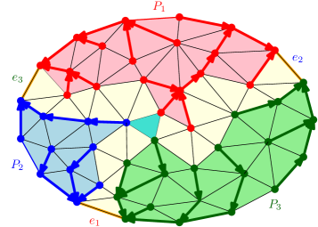
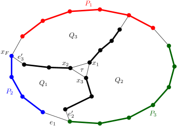
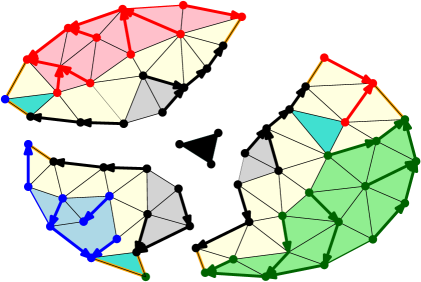
Figure 1: A single recursive step from Dujmović et al.  [5].

By the time the recursive invocation terminates, each vertex of $N-V(F)$ is included in some part of the partition $\mathcal{P}$. Let $f$ denote the number of inner triangular faces of $N$. The base case occurs when $f=1$ so $N$ consists of a single triangle ($F$). In this case (P3) implies that each vertex of $N$ is already included in $\mathcal{P}$ and there is nothing to do so the algorithm returns immediately.

If $f>1$, the paths $P_{1}$, $P_{2}$, and $P_{3}$, along with the breadth-first search tree $T$ are used to partition the vertices of $N$ into three colour classes, as follows. Each vertex $v\in P_{i}$ has colour $c(v)=i$. For each vertex $v\in V(N)\setminus V(F)$, (P1) implies that $P_{T}(v)$ contains some first vertex $v_{F}$ of $F$. The vertex $v$ is assigned the colour $c(v)=c(v_{F})$.

By Sperner’s Lemma, $N$ contains a triangular face $\tau=x_{1}x_{2}x_{3}$ that is trichromatic, i.e., $c(x_{i})=i$ for each $i\in\{1,2,3\}$. (Note that $0$, $1$, $2$, or $3$ vertices of $\tau$ may be in $V(F)$.) The edges of $F$, $\tau$, and the paths in $T$ from each $x_{i}$ to the first vertex of $P_{i}$ define a graph $M$ with at most 4 interior faces, one of which is $\tau$. Each of the other (at most three) interior faces does not contain $x_{i}$ for some $i\in\{1,2,3\}$. For each $i\in\{1,2,3\}$, we let $Q_{i}$ denote the interior face of $M$ that does not contain $x_{i}$. Observe that, for each $i\in\{1,2,3\}$, $Q_{i}$ contains no vertex of $P_{i}$.

For each $i\in\{1,2,3\}$, let $Z_{i}$ be the path, in $T$, from $x_{i}$ up to, but not including, the first vertex in $P_{i}$. Note that $Z_{i}$ may be empty, which occurs when $x_{i}$ is a vertex of $P_{i}$. Let $Y:=V(Z_{1})\cup V(Z_{2})\cup V(Z_{3})$. The algorithm adds $V(Z_{1})$, $V(Z_{2})$ and $V(Z_{3})$ to the partition $\mathcal{P}$ and then recurses on each of $Q_{1}$, $Q_{2}$, and $Q_{3}$.

We now argue that $Q_{1}$ satisifies preconditions (P1)–(P3). The face $Q_{1}$ is a cycle in $G$ that is contained in the cycle $F$, so $Q_{1}$ satisifies precondition (P1). The vertices of $Q_{1}$ are contained in $V(P_{2})\cup V(P_{3})\cup Y$. Therefore every vertex of $Q_{1}$ is contained in some part of $\mathcal{P}$, so $Q_{1}$ satisfies precondition (P3).

Let $v$ be any vertex in the interior of $Q_{1}$ and let $w$ be any $T$-descendant of $v$. In order to show that $Q_{1}$ satisfies precondition (P2) we must show that $w$ is in the interior of $Q_{1}$. If $w$ is not in the interior of $Q_{1}$ then the path in $T$ from $w$ to $v$ contains a vertex $v^{\prime}\in V(Z_{2})\cup V(Z_{3})\cup V(F)$. Since $v^{\prime}$ is a $T$-descendant of $v$, precondition (P2) implies that $v^{\prime}\not\in V(F)$. If $v^{\prime}\in V(Z_{i})$ for some $i\in\{2,3\}$, then the path from $w$ to $v$ in $T$ contains the subpath of $Z_{i}$ beginning at $v^{\prime}$ and continuing to the last vertex $v^{\prime\prime}$ of $Z_{i}$. The path from $w$ to $v$ in $T$ also contains the $T$-parent $v^{\prime\prime\prime}$ of $v^{\prime\prime}$. This again contradicts (P2) because, by definition, $v^{\prime\prime\prime}\in V(F)$ and is a $T$-descendant of $v$. Therefore every $T$-descendant $w$ of $v$ is contained in the interior of $Q_{1}$, so $Q_{1}$ satisfies precondition (P2).

Next we describe the three portals used when recursing on $Q_{1}$. The cycle $Q_{1}$ contains at least one vertex each from $V(P_{2})$ and $V(P_{3})$ and therefore also contains the portal $e_{1}$, which is also used as one of the three portals in the recursive invocation. If $V(Z_{2})\cup V(Z_{3})$ is non-empty, then $Q_{1}$ contains two edges $e_{2}^{\prime}$ and $e_{3}^{\prime}$ where $e_{2}^{\prime}$ has an endpoint in $V(P_{3})$ and an endpoint in $V(Z_{2})\cup V(Z_{3})$ and where $e_{3}^{\prime}$ has an endpoint in $V(P_{2})$ and an endpoint in $V(Z_{2})\cup V(Z_{3})$. In this case, the edges $e_{1}$, $e_{2}^{\prime}$, and $e_{3}^{\prime}$ are used as the three portals in the recursive invocation on $Q_{1}$. Note that $e_{1}$, $e_{2}^{\prime}$ and $e_{3}^{\prime}$ satisfy precondition (P4) since the vertices of $P_{1}^{\prime}$—the path from $e_{2}^{\prime}$ to $e_{3}^{\prime}$ on $Q_{1}$ that does not contain $e_{1}$—are contained in the union of $V(Z_{2})$ and $V(Z_{3})$, which are included in $\mathcal{P}$.

If $(V(Z_{2})\cup V(Z_{3}))$ is empty—because $x_{2}\in V(P_{2})$ and $x_{3}\in V(P_{3})$—then we artifically create two portals $e_{2}^{\prime}$ and $e_{3}^{\prime}$ for the recursive invocation by taking any two edges of $Q_{1}$ other than $e_{1}$. Clearly, this choice of $e_{2}^{\prime}$ and $e_{3}^{\prime}$ also satisfies precondition (P4).

The recursive invocations on $Q_{2}$ and $Q_{3}$ are done similarly, but rotating the values $1,2,3$. After these three recursive invocations, every vertex in $N-V(F)$ is included in some part of $P$, so the recursive invocation is complete.

2.1 Running-Time Analysis

Recall that $f$ denotes the number of inner faces in the near-triangulation $N$. By having each vertex of $G$ store a pointer to its parent in $T$ and storing $G$ using a representation that simultaneously represents $G$ and its dual graph $G^{*}$, the colouring of the vertices of $N$ can be done in $O(f)$ time and then the inner triangular faces of $N$ can be traversed in $O(f)$ time to find the trichromatic triangle $\tau$. The rest of the work (adding $Z_{1}$, $Z_{2}$, and $Z_{3}$ to $P$ and preparing the recursive invocations on $Q_{1}$, $Q_{2}$, and $Q_{3}$) is also easily implemented in $O(f)$ time, so the running time of the algorithm is given by the recurrence

$$T(f)\le\cases{a}&\text{forf\le 1}\\ a\cdot f+T(f_{1})+T(f_{2})+T(f_{3})\text{forf\ge 2}$$

where $a$ is a sufficiently large constant and, for each $i\in\{1,\ldots,3\}$, $f_{i}$ is the number of faces of $G$ contained in the interior of $Q_{i}$. Note that $f_{1}+f_{2}+f_{3}=f-1$ (since $\tau$ is not contained in $Q_{1}$, $Q_{2}$, or $Q_{3}$). An easy inductive proof shows that $T(f)\le a\cdot f\cdot(f+1)/2=O(f^{2})$.

The recursive procedure described above is used to prove Theorem 3 as follows. Given an $n$-vertex triangulation $G$ and a spanning tree $T$ of $G$:

1. Define one of the faces incident to the root $r$ of $T$ to be the outer face of $G$ and let $r$, $x$, and $y$ denote the three vertices on the outer face of $G$.

2. Place $\{r\}$, $\{x\}$, and $\{y\}$ in the partition $\mathcal{P}$ and run the recursive procedure described above on the cycle $F:=rxy$ with the portals $e_{1}=rx$, $e_{2}=xy$ and $e_{3}=yr$.

The first step of this procedure runs in constant time. The second step requires $\Theta(f^{2})=\Theta(n^{2})$ time in the worst case.

2.2 Treewidth Analysis

Dujmović et al. [5] show that the contraction $H:=N/\mathcal{P}$ has treewidth at most 8. Although it is not necessary to repeat their argument here, it is worth doing so because it illustrates that a width-$\le\!8$ tree decomposition of $H$ can be easily computed during the construction of the partition $\mathcal{P}$. (See Diestel [3, Chapter 12] for definitions of treewidth and tree decompositions.)

The argument mirrors the inductive structure of the algorithm used to create $\mathcal{P}$. Specifically, the recursive invocation on $F$ takes as input the set $X$ (guaranteed by (P4)) of at most 6 parts of $\mathcal{P}$ that cover $V(F)$ and produces a tree decomposition of $N/\mathcal{P}$ that has some bag $B$ containing $X$ and in which every bag has size at most $9$.

For each $i\in\{1,2,3\}$, the at most 4 parts in $X$ that cover $V(F-P_{i}))$ (again, guaranteed by (P4)) and the two parts $V(Z_{j})$, $j\in\{1,2,3\}\setminus\{i\}$ are used as the input $X_{i}$ to the recursive call on the cycle $Q_{i}$ that bounds the near-triangulation $N_{i}$. This produces a tree decomposition of $N_{i}/\mathcal{P}$ in which some bag $B_{i}$ contains $X_{i}$ and every bag has size at most $9$.

The three tree decompositions of $N_{1}$, $N_{2}$, and $N_{3}$ are then joined by introducing a bag $B:=X\cup\{V(Z_{1}),V(Z_{2}),V(Z_{3})\}$ and making $B$ adjacent to $B_{i}$ for each $i\in\{1,2,3\}$. It is straightforward to verify that this does indeed give a tree decomposition of $N/\mathcal{P}$. The bag $B$ has size $|X|+3\le 9$ and (inductively) every other bag has size at most 9, thus proving that the treewidth of $N/\mathcal{P}$ is at most 8.

We note that this tree decomposition of $H$ can be computed at the same time as the partition $\mathcal{P}$ without contributing more than $O(|V(H)|)\subseteq O(n)$ to the running time of the algorithm.

3 A Faster Algorithm

To obtain a faster algorithm we will create an algorithm (part of) whose running time satisifies the recurrence:

$$T(f)\le\cases{a}&\text{forf\le 1}\\ a\cdot(1+\min\{f_{1},f_{2},f_{3}\})+T(f_{1})+T(f_{2})+T(f_{3})\text{forf\ge 2}$$

It is straightforward to show, by induction, that $T(f)\le(a/3)f\log_{3}(f)=O(a\cdot f\log f)$. The value of $a$ here depends on the running time of an operation on a certain data structure described next.

Our algorithm makes use of a data structure that preprocesses a $(n+1)$-vertex tree $T$ with root $r$ so that it can maintain a set $S\subseteq V(T)$ that, initially, contains only $r$, and supports the following operations that each take a node $w\in V(T)$ as an argument:

• $\textsc{Mark}(w)$: Add $w$ to the set $S$. A precondition of this operation is that the parent, $v$, of $w$ is already in $S$ but $w$ is not yet in $S$.

• $\textsc{NearestMarkedAncestor}(w)$: Return the first node $v\in S$ that is on the path from $w$ to the root of $T$.

In Appendix A we show how to use standard techniques to obtain the following result:

Lemma 4.

There exists a data structure that preprocesses any $n$-node rooted tree $T$ and supports the $\textsc{Mark}(w)$ and $\textsc{NearestMarkedAncestor}(w)$ operations. Each $\textsc{NearestMarkedAncestor}(w)$ operation takes $O(1)$ time and any sequence of $\textsc{Mark}(w)$ operations takes a total of $O(n\log n)$ time.

In the remainder of this section, we will show how Lemma 4 can be used to achieve the desired running time. It is worth noting that the algorithm we now describe has the same recursion tree and produces exactly the same partition $\mathcal{P}$ as the original algorithm. Therefore $\mathcal{P}$ has all the properties described by Dujmović et al.. [5]. In particular, the quotient graph $H:=G/\mathcal{P}$ has treewidth at most $8$ and a tree decomposition of $H$ of widtch at most $8$ can be computed while computing $\mathcal{P}$.

As before, each recursive step takes as input the cycle $F$ and the three portals $e_{1}$, $e_{2}$, and $e_{3}$. Additionally, the algorithm requires that the vertices of $P_{1}$, $P_{2}$ and $P_{3}$ are coloured with three different colours. More precisely, there are three distinct integers $c_{1}$, $c_{2}$ and $c_{3}$ such that $c(v)=c_{i}$ for each $v\in V(P_{i})$ and each $i\in\{1,2,3\}$. The nearest marked ancestor data structure maintaining $S\subseteq V(T)$ is set up so that $V(F)\subseteq S$ and $(V(N)\setminus V(F))\cap S=\emptyset$. That is, $S$ contains all vertices on the outer face of $N$, but none of the inner vertices.

The algorithm searches for the trichromatic triangle $\tau$ beginning from the portals. Refer to Figure 2. Step 0 of the search begins with $e_{i,0}=e_{i}$ and $t_{i,0}$ as the unique triangular inner face of $N$ with $e_{i}$ on its boundary, for each $i\in\{1,2,3\}$. In Step $j$ of the search, the algorithm has three triangles $t_{i,j}$ and three edges $e_{i,j}$ where $e_{i,j}$ is an edge of $t_{i,j}$ for each $i\in\{1,2,3\}$. Using the data structure for $T$, the algorithm checks, for each $i\in\{1,2,3\}$, the colours of $t_{i,j}$’s three vertices by calling $\textsc{NearestMarkedAncestor}(w)$ for each of $t_{i,j}$’s three vertices. This returns a vertex $v\in V(F)$ whose colour gives the colour of $w$.

If $t_{i,j}$ is trichromatic for at least one $i\in\{1,2,3\}$, then the algorithm has found the necessary trichromatic triangle $\tau$ and this step is complete. Otherwise, for each $i\in\{1,2,3\}$, the triangle $t_{i,j}$ contains another bichromatic edge $e_{i,j+1}\neq e_{i,j}$ and this edge bounds another triangular face $t_{i,j+1}\neq t_{i,j}$ of $N$. The algorithm then continues to Step $(j+1)$ of the search using the triangles $t_{i,j+1}$ and edges $e_{i,j+1}$ for each $i\in\{1,2,3\}$. The fact that this algorithm terminates (and would terminate even if the search were limited to any one of the portals) follows from a classic proof of Sperner’s Lemma in two dimensions.

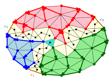
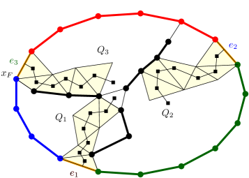
Figure 2: Searching for the trichromatic triangle $\tau$ beginning at the portals $e_{1}$, $e_{2}$, and $e_{3}$. In this example, $\tau=t_{1,6}$ is found after $k+1=7$ steps.

Suppose the search for $\tau$ succeeds when $\tau=t_{i,k}$ in Step $k$. Thus, for each $i\in\{1,2,3\}$, the algorithm has searched the sequence of triangles $t_{i,0},\ldots,t_{i,k}$. Each of the shorter subsequences $S_{i}:=t_{i,0},\ldots,t_{i,k-1}$ consists entirely of bichromatic triangles. Each sequence $S_{i}$ contains $k$ bichromatic triangles whose vertices are coloured with $\{c_{1},c_{2},c_{3}\}\setminus c_{i}$.

Refer to the second part of Figure 2. Consider again the graph $M$ with inner faces $Q_{1}$, $Q_{2}$, $Q_{3}$ and $\tau$. For each $i\in\{1,2,3\}$, each face in $S_{i}$ is contained in $Q_{i}$. Since $f_{i}$ counts the number of triangular faces of $N$ contained in $Q_{i}$, this implies that $f_{i}\ge k$ for each $i\in\{1,2,3\}$. Therefore, $\min\{f_{1},f_{2},f_{3}\}\ge k$. On the other hand, the search for for $\tau$ took $1+k$ steps, each of which performs three $\textsc{NearestMarkedAncestor}(w)$ queries and therefore the entire search runs in time $O(1+k)\subseteq O(1+\min\{f_{1},f_{2},f_{3}\})$.

Next, the algorithm prepares the three subproblems defined by $Q_{1}$, $Q_{2}$, and $Q_{3}$ on which to recurse. To do this it follows the path $Z_{i}$, in $T$, from each vertex $x_{i}$ of $\tau$ to the first vertex of $P_{i}$. It colours each vertex of $z_{i}$ with some colour $c_{4}\not\in\{c_{1},c_{2},c_{3}\}$ and then walks $Z_{i}$ backward, calling $\textsc{Mark}(w)$ for each vertex of $Z_{i}$.

Finally, in preparing each subproblem $Q_{i}$ for the recursive invocation, it may be necessary to change the colour of an already coloured vertex $v$ of $F$ with the colour $c_{4}$ before making the recursive call and then recolouring $v$ with its original colour once the recursion is complete. This corresponds to introducing an artificial portal adjacent to an edge of $\tau$ contained in $F$.

3.1 Running-Time Analysis

We analyze the running time of the preceding algorithm by analyzing two parts separately.

During each recursive invocation, the algorithm does work to find the trichromatic triangle $\tau$. The time associated with this is $O(1+k)$ where $k\ge\min\{f_{1},f_{2},f_{3}\}$. As already described above, this leads to a recurrence of the form $T(f)\le O(\min\{f_{1},f_{2},f_{3}\})+T(f_{1})+T(f_{2})+T(f_{3})$ which resolves to $O(f\log f)$. In the initial call, $f=2n-3$ is the number of inner faces of $G$, so the total running time attributable to this part of the algorithm is $O(n\log n)$.

In addition to this, the algorithm does other work in preparing inputs for recursive calls. Once $\tau$ is identified, the previously uncoloured vertices of $Y$ are coloured. A vertex $v\in V(G)$ appears in $Y$ during exactly one recursive invocation. Thus, colouring the vertices of $Y$ contributes a total of $O(n)$ time to the running time of the entire algorithm.

Finally, the vertices of $Y$ are added to the set $S$ maintained by the nearest marked ancestor data structure using calls to $\textsc{Mark}(w)$. By Lemma 4, this takes a total of $O(n\log n)$ time. This completes the proof of the following theorem:

Theorem 5.

There exists an algorithm that, given any $n$-vertex triangulation $G$ and any breadth-first-search tree $T$ of $G$, runs in $O(n\log n)$ time and finds a partition $\mathcal{P}$ of $V(G)$ such that each $P\in\mathcal{P}$ induces a vertical path in $T$ and the quotient graph $H:=G/\mathcal{P}$ has treewidth at most $8$.

4 Discussion

Another variant of Theorem 3 described by Dujmović et al. gives a partition $\mathcal{P}$ of $V(G)$ such that $G/\mathcal{P}$ has treewidth at most 3 and each part $Y\in\mathcal{P}$ is the union of at most 3 vertical paths in $T$. The algorithm described here also gives an $O(n\log n)$ time algorithm for this variant.

4.1 Other Graph Classes

Theorem 1 has been generalized to a number of graph classes including bounded-genus graphs [5], apex-minor free graphs [5], graphs of bounded-degree from proper-minor closed families [4], and $k$-planar graphs [7]. In all cases, these generalizations ultimately involve decomposing the input graph into a number of planar subgraphs and applying Theorem 1 to each of these planar graphs.

In at least two cases, the extra work done in these generalizations can be done in $O(n\log n)$ time. Combined with Theorem 2, this gives $O(n\log n)$ time algorithms for the corresponding generalizations of Theorem 1.

• For graphs $G$ of fixed Euler genus $g$, the result of Dujmović et al. [5] only requires finding a genus-$g$ embedding of $G$, computing a breadth-first-search tree $T$ of $G$, and computing any spanning-tree $D$ of the dual graph that does not cross edges of $T$. The two spanning trees $T$ and $D$ can be computed in $O(n)$ time using standard algorithms. The genus-$g$ embedding of $G$ can be computed in $O(n)$ time using an algorithm of Mohar [15]

• Given a $k$-plane embedding of a $k$-planar graph $G$, the result of Dujmović, Morin, and Wood [7] applies Theorem 1 directly to the planar graph obtained by adding a dummy vertex at every point where a pair of edges crosses.

  While the problem of testing $k$-planarity of a graph is NP-complete, even for $k=1$ [9, 13, 19], there are a number of graph classes that are $k$-planar and in which an embedding can be found easily. These include (appropriate representations of) map graphs, bounded-degree string graphs, powers of bounded-degree planar graphs, and $k$-nearest-neighbour graphs of points in $\mathbb{R}^{2}$ [7, Section 8].

4.2 Applications

The algorithm presented here applies immediately to the four applications of Theorem 1 discussed in the introduction.

• There exists an algorithm that, given an $n$-vertex planar graph $G$, runs in $O(n\log n)$ time and computes a 49 queue layout of $G$ [5].

• There exists an algorithm that, given an $n$-vertex planar graph $G$, runs in $O(n\log n)$ time and computes a nonrepetitive colouring of $G$ using at most 768 colours [4].

• There exists an algorithm that, given an $n$-vertex planar graph $G$, runs in $O(n\log n)$ time and computes a $(1+o(1))\log n$-bit adjacency labelling of $G$ [6].

• There exists an algorithm that, given an $n$-vertex planar graph $G$ and an integer $p$, runs in $O(p^{3}n\log n)$ time and computes $p$-centered colouring of $G$ using at most $3(p+1)\binom{p+3}{3}$ colours [2].

Prior to this work, the bottleneck in all these algorithms was the $\Theta(n^{2})$ worst-case running time of the algorithm for computing the decomposition of Theorem 1.

4.3 Future Work

The obvious open problem left by our work is that of finding a faster algorithm. Can the running-time in Theorem 2 be improved to $O(n)$?

Appendix A Data Structures

In this appendix we describe the simple data structures used by our algorithm. Devising these data structures is an exercise in the use of two standard techniques (a simple union-find data structure and the interval labelling scheme for rooted trees).

A.1 Interval Splitting

An interval splitting data structure stores an initially-empty subset $S$ of $\{1,\ldots,n\}$ under the following two operations, each of which takes an integer argument $x\in\{1,\ldots,n\}$:

• $\textsc{Add}(x)$: Add $x$ to the set $S$, i.e., $S\leftarrow S\cup\{x\}$. It is a precondition of this operation that $x\not\in S$.

• $\textsc{Interval}(x)$: Return the pair $(i,j)$ where $i=\max\{y\in S\cup\{0\}:y<x\}$ and $j=\min\{y\in S\cup\{n+1\}:y\ge x\}$.

Lemma 6.

There exists a data structure that preprocesses an integer $n$ and supports the $\textsc{Add}(x)$ and $\textsc{Interval}(x)$ operations. The data structures uses $O(n)$ preprocessing time, each $\textsc{Interval}(x)$ operation runs in $O(1)$ time and any sequence of $\textsc{Add}(x)$ operations takes a total of $O(n\log n)$ time.

Proof.

The data structure is essentially the inverse of one of the simplest union-find data structures that represents sets as linked lists in which each node has a pointer to the head of the list.

The data structure contains an array $a_{1},\ldots,a_{n}$ of pointers. For each $x\in\{1,\ldots,n\}$, the array entry $a_{x}$ points to a memory location $m$ storing the interval $(i,j)$ that answers the $\textsc{Interval}(x)$ query. In this way each $\textsc{Interval}(x)$ query operation runs in $O(1)$ time, as required.

The data structure is memory-efficient in the following sense: Suppose that, at some point in time $S=\{x_{1},\ldots,x_{k}\}$ with $x_{1}<\cdots<x_{k}$. and use the convention that $x_{0}:=0$ and $x_{k+1}=n+1$. Then, for each $i\in\{0,\ldots,k\}$, the array locations $a_{x_{i}+1},\ldots,a_{\min\{n,x_{i+1}\}}$ all point the same memory location $m$ that contains the pair $(i,j)$, $i<x\le j$ that answers the $\textsc{Interval}(x)$ query for each value $x\in\{x_{i}+1,\ldots,x_{i+1}\}$. Thus, the number of distinct memory locations $m$ used to store answers to $\textsc{Interval}(x)$ queries is exactly $k+1$.

To perform an $\textsc{Add}(x)$ operation, the data structure first looks at the pair $(i,j)$ stored at the memory location $m$ referenced by $a_{x}$. Observe that the $j-i$ array entries $a_{i+1},\ldots,a_{j}$ all point to the same memory location $m$ and let $k:=x-i$. The data structure allocates a new memory location $m^{\prime}$ containing a pair $(i^{\prime},j^{\prime})$. The algorithm then makes a choice, depending on the value of $k$.

1. If $k\le(j-i)/2$, then it sets $(i^{\prime},j^{\prime})\leftarrow(i,x)$, sets $(i,j)\leftarrow(x,j)$ and sets $a_{i+1},\ldots,a_{x}\leftarrow m^{\prime}$.

2. Otherwise, it sets $(i^{\prime},j^{\prime})\leftarrow(x,j)$, sets $(i,j)\leftarrow(i,x)$ and sets $a_{x+1},\ldots,a_{j}\leftarrow m^{\prime}$.

It is straightforward to verify that these operations are correct.

To analyze total running time of a sequence of $\textsc{Add}(x)$ operations, we use the potential method of amortized analysis. For each $\ell\in\{1,\ldots,n\}$, let $\Phi_{\ell}=c\log_{2}(j-i)$ where $(i,j)$ is the answer to $\textsc{Interval}(\ell)$ and let $\Phi=\sum_{\ell=1}^{n}\Phi_{\ell}$. Observe that $0\le\Phi_{\ell}\le c\log_{2}(n+1)$ for each $\ell\in\{1,\ldots,n\}$, so $0\le\Phi\le cn\log_{2}(n+1)$. Note, furthermore that the $\textsc{Interval}(x)$ operation has no effect on $\Phi$.

When an $\textsc{Add}(x)$ operation runs, it updates some number $z$ of array entries (either $z=k$ or $z=j-i-k$. This takes $O(z)$ time and does not cause $\Phi_{\ell}$ to increase for any $\ell\in\{1,\ldots,n\}$. Furthermore, this operation causes $\Phi_{\ell}$ to decrease by at least $c$ for each array entry $a_{\ell}$ that is modified. Therefore, letting $\Phi$ and $\Phi^{\prime}$ denote the value of $\Phi$ before and after this operation, we have $\Phi^{\prime}-\Phi\le-cz$. The amortized running time of this operation is therefore $O(1+z+\Phi^{\prime}-\Phi)=O(1)$ for a sufficiently large constant $c$.

Therefore each $\textsc{Add}(x)$ operation runs in $O(1)$ amortized time, the minimum potential is $0$ and the maximum potential is $cn\log_{2}(n+1)$, so the total running time of any sequence of $\textsc{Add}(x)$ operations is at most $O(m+n\log n)$. The precondition that $x\not\in S$ ensures that $m\le n$, so the total running time is $O(n\log n)$. ∎

A.2 Nearest Marked Ancestor

Proof of Lemma 4.

The data structure is essentially the interval labelling scheme for trees combined with the interval splitting data structure from the previous section.

Let $T^{\prime}$ be the directed graph obtained by replacing each undirected edge $vw$ of $T$ with two directed edges $vw$ and $wv$. Since every node of $T^{\prime}$ has the same in and out degree, it is Eulerian. Let $v_{1},v_{2},\ldots,v_{2n-1}$ be the sequence of vertices encountered during an Euler tour of $T^{\prime}$ that begins and ends at the root $v_{1}=v_{2n-1}$ of $T$. For each node $v$ of $T$, let $i_{v}:=\min\{i:v_{i}=v\}$ and $j_{v}:=\max\{j:v_{j}=v\}$. Observe that $v_{i_{v}},v_{i_{v}+1},\ldots,v_{j_{v}}$ contains exactly those nodes of $T$ that have $v$ as a $T$-ancestor.

The data structure stores the sequence $v_{0},v_{1},v_{2},\ldots,v_{2n-1}$ in an array and maintains an interval splitting data structure on the set $1,\ldots,2n-1$. The operation of $\textsc{Mark}(w)$ is simple: We simply call $\textsc{Add}(i_{w})$ and $\textsc{Add}(j_{w})$. Note that the precondition that $w\not\in S$ ensures that the precondition $x\not\in S$ of the $\textsc{Add}(x)$ operation is satisified. Thus, any sequence of $\textsc{Mark}(w)$ operations results in a sequence of $\textsc{Add}(x)$ operations on the set $\{1,\ldots,2n-1\}$. By Lemma 6 this takes a total of $O(n\log n)$ time, as required.

The operation of the $\textsc{NearestMarkedAncestor}(v)$ is almost as simple. We call $\textsc{Interval}(i_{w})$ to obtain some pair $(i,j)$ with $i<i_{w}\le j$. There are two cases to consider:

1. If $j=i_{w}$ then this is because $w\in S$, in which case $w$ is the nearest marked ancestor of itself.

2. Otherwise, $i<i_{w}<j$, and $(i,j)=(i_{v},j_{v})$ for some node $v\in S$. Therefore, $v_{i}=v_{j}$ is the nearest marked ancestor of $w$.

Therefore, in either case, we obtain the nearest marked ancestor of $w$ in $O(1)$ time, as required. ∎

References

- [1] Noga Alon, Jarosław Grytczuk, Mariusz Hałuszczak, and Oliver Riordan. Nonrepetitive colorings of graphs. Random Structures Algorithms, 21(3-4):336–346, 2002. doi:10.1002/rsa.10057.
- [2] Michał Dębski, Stefan Felsner, Piotr Micek, and Felix Schröder. Improved bounds for centered colorings. In Shuchi Chawla, editor, Proceedings of the 2020 ACM-SIAM Symposium on Discrete Algorithms, SODA 2020, Salt Lake City, UT, USA, January 5-8, 2020, pages 2212–2226. SIAM, 2020. doi:10.1137/1.9781611975994.136.
- [3] Reinhard Diestel. Graph Theory, Fifth Edition, volume 173 of Graduate texts in mathematics. Springer, 2017. doi:10.1007/978-3-662-53622-3.
- [4] Vida Dujmović, Louis Esperet, Gwenaël Joret, Bartosz Walczak, and David R. Wood. Planar graphs have bounded nonrepetitive chromatic number. Advances in Combinatorics, March 2020. doi:10.19086/aic.12100.
- [5] Vida Dujmovic, Gwenaël Joret, Piotr Micek, Pat Morin, Torsten Ueckerdt, and David R. Wood. Planar graphs have bounded queue-number. J. ACM, 67(4):22:1–22:38, 2020. URL: https://dl.acm.org/doi/10.1145/3385731.
- [6] Vida Dujmović, Louis Esperet, Cyril Gavoille, Gwenaël Joret, Piotr Micek, and Pat Morin. Adjacency labelling for planar graphs (and beyond). CoRR, abs/2003.04280, 2020. URL: https://arxiv.org/abs/2003.04280, arXiv:2003.04280.
- [7] Vida Dujmović, Pat Morin, and David R. Wood. The structure of k-planar graphs. CoRR, abs/1907.05168, 2019. URL: http://arxiv.org/abs/1907.05168, arXiv:1907.05168.
- [8] Harold N. Gabow and Robert Endre Tarjan. A linear-time algorithm for a special case of disjoint set union. J. Comput. Syst. Sci., 30(2):209–221, 1985. doi:10.1016/0022-0000(85)90014-5.
- [9] Alexander Grigoriev and Hans L. Bodlaender. Algorithms for graphs embeddable with few crossings per edge. Algorithmica, 49(1):1–11, 2007. doi:10.1007/s00453-007-0010-x.
- [10] Lenwood S. Heath, F. Thomson Leighton, and Arnold L. Rosenberg. Comparing queues and stacks as mechanisms for laying out graphs. SIAM J. Discrete Math., 5(3):398–412, 1992. doi:10.1137/0405031.
- [11] Sampath Kannan, Moni Naor, and Steven Rudich. Implicit representation of graphs. In Janos Simon, editor, Proceedings of the 20th Annual ACM Symposium on Theory of Computing, May 2-4, 1988, Chicago, Illinois, USA, pages 334–343. ACM, 1988. doi:10.1145/62212.62244.
- [12] Sampath Kannan, Moni Naor, and Steven Rudich. Implicit representation of graphs. SIAM J. Discrete Math., 5(4):596–603, 1992. doi:10.1137/0405049.
- [13] Vladimir P. Korzhik and Bojan Mohar. Minimal obstructions for 1-immersions and hardness of 1-planarity testing. Journal of Graph Theory, 72(1):30–71, 2013. doi:10.1002/jgt.21630.
- [14] Dan Kráľ and Ranko Lazic. Open problems from the workshop on algorithms, logic and structure, December 2016. URL: https://warwick.ac.uk/fac/sci/maths/people/staff/daniel_kral/alglogstr/openproblems.pdf.
- [15] Bojan Mohar. A linear time algorithm for embedding graphs in an arbitrary surface. SIAM J. Discrete Math., 12(1):6–26, 1999. doi:10.1137/S089548019529248X.
- [16] Jaroslav Nešetřil and Patrice Ossona de Mendez. Tree-depth, subgraph coloring and homomorphism bounds. Eur. J. Comb., 27(6):1022–1041, 2006. doi:10.1016/j.ejc.2005.01.010.
- [17] Jaroslav Nešetřil and Patrice Ossona de Mendez. Grad and classes with bounded expansion i. decompositions. Eur. J. Comb., 29(3):760–776, 2008. doi:10.1016/j.ejc.2006.07.013.
- [18] Michał Pilipczuk and Sebastian Siebertz. Polynomial bounds for centered colorings on proper minor-closed graph classes. In Timothy M. Chan, editor, Proceedings of the Thirtieth Annual ACM-SIAM Symposium on Discrete Algorithms, SODA 2019, San Diego, California, USA, January 6-9, 2019, pages 1501–1520. SIAM, 2019. arXiv:1807.03683v2, doi:10.1137/1.9781611975482.91.
- [19] John C. Urschel and Jake Wellens. Testing k-planarity is NP-complete. CoRR, abs/1907.02104, 2020. arXiv:1907.02104.