Helicity form factors for $D_{(s)}\to A\ell\nu$ process in the light-cone QCD sum rules approach

Abstract

The helicity form factors of the $D_{(s)}\to A\ell^{+}\nu$ with $A=a_{1}^{-},a_{1}^{0},b_{1}^{-},b_{1}^{0},K_{1}(1270)$ and $K_{1}(1400)$ are calculated in the light-cone sum rules approach, up to twist-3 distribution amplitudes of the axial vector meson $A$. In the helicity form factors parametrization the unitarity constraints are applied to the fitting parameters. In addition, the effects of the low-lying resonances are included in series expansions of aforementioned form factors. The properties of the $D_{(s)}\to A\ell^{+}\nu$ semileptonic decays are studied by extending the form factors to the whole physical region of $q^{2}$. For a better analysis, a comparison is also made between our results and the predictions obtained using transition form factors via LCSR, 3PSR and CLFQM methods.

I Introduction

The weak semileptonic and hadronic decays of charmed mesons, which occur in the presence of strong interaction, are ideal laboratory candidates to determine the quark mixing parameters and the values of the Cabibbo-Kobayashi-Maskawa (CKM) matrix elements and establish new physics beyond the standard model (SM). These meson category masses are $(\mathcal{O}~{}2~{}\rm{GeV})$, therefore charm decays are helpful to study nonperturbative QCD while, the heavy quark effective theory (HQET) can also be utilized to study $D$ meson decays Artuso .

$D_{(s)}$ meson decays can be classified into two categories. The first one, which occurs via $c\to u~{}\ell^{+}\ell^{-}$ transition at quark level, is named the flavor changing neutral currents (FCNC) decay. The $D\to\pi\ell^{+}\ell^{-}$, $D\to\rho\ell^{+}\ell^{-}$, $D\to\pi\,\gamma$ and $D\to\rho\,\gamma$ from the first group, are studied using QCD factorization Feldmann . The second class, which happens by the semileptonic decay of charm quark $c\to d(s)\ell\nu$ are analyzed via different approaches. Traditionally, semileptonic decays are explained in terms of transition form factors as a function of the invariant mass of the electron-neutrino pair, $q^{2}$. These form factors which parameterize nonperturbative effects, are measured for $D\to K\ell\nu$ decay in Zhang , while, the Light Cone QCD Sum Rule (LCSR) approach is utilized to studying $D\to\pi(K,\rho)\,\ell\,\nu$ decays Khodjamirian ; BallD ; Fu . The form factors of the $D^{+}\to(D^{0},\rho^{0},\omega,\eta,\eta^{\prime})\ell^{+}\nu$ and $D^{+}_{s}\to(D^{0},\phi,K^{0},K^{*0},\eta,\eta^{\prime})\ell^{+}\nu$ semileptonic decays have been calculated in the framework of the covariant confined quark model (CCQM) Soni1 ; Soni2 . The semileptonic decays $D\to(\pi,\rho,K,K^{*})\ell\nu$ have been studied using the (HQET) in Ref. WangD and the lattice QCD (LQCD) results for the $D\to\pi(K,K^{*})\ell\,\nu$ processes are reported in Abada ; Aubin ; Bernard . In Ref. Ignacio ; Aliev ; Ball2 ; Ball3 ; Ovchinnikov ; Dong ; Mao the semileptonic decays $D_{(s)}\to f_{0}(K_{0}^{*})\,\ell\,\nu$, $D_{(s)}\to\pi(K)\,\ell\,\nu$, and $D_{(s)}\to K^{*}(\rho,\phi)\,\ell\,\nu$ have been investigated in the framework of the three-point QCD sum rules (3PSR). The $D\to\,a_{1},f_{1}(1285),f_{1}(1420)$ and $D_{(s)}\to K_{1}\,\ell\,\nu$ transitions as the $D_{(s)}$ decay to the axial vector mesons, have been calculated by the 3PSR method Khosravi ; Zuo .

In this paper, the helicity form factors for the $D_{(s)}$ decays into axial vectors are calculated with the LCSR. The helicity form factors which can be obtained by contracting the $W(\rm{or}~{}Z)$ boson polarization vectors and the transition matrix elements, are also functions of $q^{2}$. The relations among the $D_{(s)}\to A$ transition matrix elements, transition form factors and the helicity ones are presented in Table 1.

Matrix element	Transition form factors	Helicity form factors
$\begin{array}[]{c}\langle A|\bar{s}(\bar{d},\bar{u})~{}\gamma^{\mu}\gamma^{5}c|D_{(s)}\rangle\\ \langle A|\bar{s}(\bar{d},\bar{u})~{}\gamma^{\mu}c|D_{(s)}\rangle\end{array}$	$\begin{array}[]{c}A\\ V_{0},V_{1},V_{2}\end{array}$	$\left\}\begin{array}[]{c}\mathcal{H}_{\mathcal{V},0}\\ \mathcal{H}_{\mathcal{V},1},~{}\mathcal{H}_{\mathcal{V},2}\end{array}\right.$
$\begin{array}[]{c}\langle A|\bar{u}~{}\sigma^{\mu\nu}\gamma^{5}q_{\nu}c|D_{(s)}\rangle\\ \langle A|\bar{u}~{}\sigma^{\mu\nu}q_{\nu}c|D_{(s)}\rangle\end{array}$	$\begin{array}[]{c}T_{1}(q^{2})\\ T_{2}(q^{2}),T_{3}(q^{2})\end{array}$	$\left\}\begin{array}[]{c}\mathcal{H}_{\mathcal{T},0}\\ \mathcal{H}_{\mathcal{T},1},~{}\mathcal{H}_{\mathcal{T},2}\end{array}\right.$

Table 1: The $D_{(s)}\to A$ decay hadronic matrix elements with the corresponding transition and helicity form factors. In this table $\mathcal{V}$ and $\mathcal{T}$ stands for the vector and tensor current, respectively.

There are some advantages in using the helicity form factors:

1) Diagonalizable unitarity relations can be imposed on the coefficients of the helicity form factor parameterization.

2) In the helicity form factors, the contributions from the excited states and the spin-parity quantum numbers are considered by relating the dominant poles in the LCSR predictions to low-lying resonances (for more detailed, see Bharucha2010 ).

The masses and quantum numbers $J^{P}$ of low-lying $D_{(s)}$ resonances with the relations among the helicity form factors are provided in Table 2. These masses will be used in the helicity form factors parameterizations. Notice that the mass values for $D_{s}(1^{-})$ and none of the $(1^{+})$ states predicted in Bardeen2003 have been experimentally confirmed yet.

		$\rm{D\,meson}$	$\rm{Mass(Gev)}$				$\rm{D\,meson}$	$\rm{Mass(Gev)}$
$\begin{array}[]{c}J^{P}=1^{-},\\ \mathcal{H}_{\mathcal{V},1}\\ \end{array}$	$\left\{\begin{array}[]{c}\\ \\ \end{array}\right.$	$\begin{array}[]{c}D^{+}\\ D^{0}\\ D_{s}\end{array}$	$\begin{array}[]{c}2.01\\ 2.00\\ 2.11\end{array}$	$\begin{array}[]{c}J^{P}=1^{+},\\ \mathcal{H}_{\mathcal{V},0},\mathcal{H}_{\mathcal{V},2}\\ \end{array}$	$\left\{\begin{array}[]{c}\\ \\ \end{array}\right.$	$\begin{array}[]{c}\\ \\ \end{array}$	$\begin{array}[]{c}D^{+}\\ D^{0}\\ D_{s}\end{array}$	$\begin{array}[]{c}2.35\\ 2.35\\ 2.46\end{array}$

Table 2: The masses of low-lying $D_{(s)}$ resonances and their relations to the helicity form factors. The masses are taken form PDG values pdg and the heavy-quark chiral symmetry approach Bardeen2003 .

In Cheng2018 , the helicity form factors are calculated via LCSR approach for $B\to\rho$ decay. In this paper, these form factors are evaluated for $D^{0}\to a^{-}_{1}(b^{-}_{1})\ell^{+}\nu$, $D^{+}\to a^{0}_{1}(b^{0}_{1})\ell^{+}\nu$ and $D_{(s)}\to K_{1}\ell^{+}\nu$ decays, which are described by $c\to d~{}\ell\nu$ transition at quark level. The form factors are also estimated for the $c\to s~{}\ell\nu$ transition in $D^{+}\to K_{1}\ell^{+}\nu$ decay. Here the physical states $K_{1}=K_{1}(1270),K_{1}(1400)$ are the mixtures of the $K_{1A}$ and $K_{1B}$ in terms of a mixing angle as Kwei2 :

$$|K_{1}(1270)\rangle = \sin\theta_{K}|K_{1A}\rangle+\cos\theta_{K}|K_{1B}\rangle,$$

$$|K_{1}(1400)\rangle = \cos\theta_{K}|K_{1A}\rangle-\sin\theta_{K}|K_{1B}\rangle,$$ (1)

where $|K_{1A}\rangle$ and $|K_{1B}\rangle$ are not mass eigenstates. The mixing angle $\theta_{K}$ is determined by various experimental analyses. The result $35^{\circ}\leq|\theta_{K}|\leq 55^{\circ}$ was reported in Ref. Burakovsky . Moreover, two possible solutions were obtained as $|\theta_{K}|\approx 33^{\circ}\vee 57^{\circ}$ in Ref. Suzuki and as $|\theta_{K}|\approx 37^{\circ}\vee 58^{\circ}$ in Ref. HYCheng . Using the study of $B\to K_{1}(1270)\gamma$ and $\tau\to K_{1}(1270)\nu_{\tau}$ decays, the value of $\theta_{K}$ is estimated as Hatanaka2

$$\theta_{K}={-(34\pm 13)}^{\circ}.$$ (2)

In this study, the branching ratio values are reported for the $D_{(s)}\to K_{1}\ell^{+}\nu$ decays at $\theta_{K}={-(34\pm 13)}^{\circ}$.

Our paper is organized as follows: In Sec. II by using the LCSR, the form factors of $D_{(s)}\to A$ decays are derived. Section. III, is devoted to the numerical analysis of the form factors and the branching ratios for semileptonic and decays. A comparison of our results for the branching ratios with the other approaches and existing experimental data is also made in this section and the last section is reserved for summary.

II Light cone QCD sum rules for $D^{0}\to a_{1}^{-}\ell\nu$ Helicity form factors

To calculate the helicity form factors of $D^{0}\to a_{1}^{-}\ell\nu$ decay, the following correlation function is considered:

$$\Pi_{\sigma}^{a_{1}}(p_{i},p_{f}) = \sqrt{\frac{q^{2}}{\lambda}}\sum_{\alpha}\varepsilon^{*\mu}_{\sigma}\int d^{4}x\,e^{iqx}\langle a_{1}^{-}(p_{f},\varepsilon_{\alpha})|{\cal{T}}\{\,j_{\mu}^{int}(x)\,j_{D^{0}}^{{\dagger}}(0)\}|0\rangle,$$ (3)

where $p_{i}$, $p_{f}=(p_{f}^{0},0,0,|\vec{p_{f}}|)$ and $q=p_{i}-p_{f}$ are the four-momentum of the $D^{0}$, $a_{1}^{-}$ and $W$-boson, respectively. Moreover, $j_{\mu}^{int}=\bar{d}\gamma_{\mu}(1-\gamma_{5})c$ is the interaction current for $D^{0}\to a_{1}^{-}$ process and $j_{D^{0}}=i{\bar{u}}\,\gamma_{5}\,c$ is the interpolating current for $D^{0}$ meson. In $\Pi_{\sigma}^{a_{1}}$ expression, $\varepsilon_{\alpha}$ and $\varepsilon_{\sigma}$ denote the polarization for $a_{1}$ meson and $W$-boson, respectively as

$$\varepsilon_{{\alpha=0}} = \frac{1}{m_{a_{1}^{-}}}(|\vec{p_{f}}|,0,0,p_{f}^{0}),$$ (4)

$$\varepsilon_{{\alpha=\pm}} = \mp\frac{1}{{\sqrt{2}}}(0,1,\mp i,0),$$ (5)

$$\varepsilon_{{\sigma=0}} = \frac{1}{{\sqrt{q^{2}}}}\,(|\vec{q}|,0,0,-q^{0}),$$ (6)

with $|\vec{p}_{f}|=\sqrt{\lambda}/2m_{D^{0}}$, $p_{f}^{0}={(m_{D^{0}}^{2}+m_{a_{1}^{-}}^{2}-q^{2})}/{2m_{D^{0}}}$, $|\vec{q}|=|\vec{p}_{f}|$ and $q^{0}={(m_{D^{0}}^{2}-m_{a_{1}^{-}}^{2}+q^{2})}/{2m_{D^{0}}}$. Also, $\lambda=(t_{-}-q^{2})(t_{+}-q^{2})$ with $t_{\pm}=(m_{D^{0}}\pm m_{a_{1}^{-}})^{2}$. Moreover, $\varepsilon_{{\sigma=\pm}}$ has similar definition as $\varepsilon_{{\alpha=\pm}}$.

For off-shell $W$-boson, $\varepsilon_{{\sigma=1}}$ and $\varepsilon_{{\sigma=2}}$ are linear combinations of the transverse $(\pm)$ polarization vectors as

$$\varepsilon_{\sigma=1} = \frac{{(\varepsilon_{\sigma=-})-(\varepsilon_{\sigma=+})}}{{\sqrt{2}}}=(0,1,0,0),$$ (7)

$$\varepsilon_{\sigma=2} = \frac{{(\varepsilon_{\sigma=-)}+(\varepsilon_{\sigma=+})}}{{\sqrt{2}}}=(0,0,i,0).$$ (8)

In the Light Cone QCD sum rules approach, the correlation function is given in Eq. (3), should be calculated in phenomenological and theoretical representations. Helicity form factors are found to equate both representations of the correlation function through dispersion relation.

The phenomenological side can be obtained by inserting a complete series of the intermediate hadronic states with the same quantum numbers as the interpolating current $j_{D^{0}}$. After separating the lowest $D^{0}$ meson ground state and applying Fourier transformation, $\Pi_{\sigma}^{a_{1}}$ is obtained as:

$$\Pi_{\sigma}^{a_{1}} = \sqrt{\frac{q^{2}}{\lambda}}\,\sum_{\alpha}{\varepsilon_{\sigma}^{*\mu}}\frac{\langle a_{1}^{-}(p_{f},\varepsilon_{\alpha})|\bar{d}\,\gamma_{\mu}(1-\gamma^{5})\,c|D^{0}\rangle\langle D^{0}|j_{D^{0}}^{{\dagger}}(0)|0\rangle}{(m_{D^{0}}^{2}-p_{i}^{2})}$$ (9)

$$+ \frac{1}{\pi}\sqrt{\frac{q^{2}}{\lambda}}\sum_{\alpha}{\varepsilon_{\sigma}^{*\mu}}\int_{0}^{\infty}\frac{\rho_{\mu}^{h}(s)}{s-p^{2}}\,ds,$$

where, $\rho_{\mu}$ is the density of higher states and continuum which can be approximated using the ansatz of the quark-hadron duality as

$$\rho_{\mu}^{h}(s)=\rho_{\mu}^{QCD}(s)\theta(s-s_{0}),$$ (10)

where, $\rho_{\mu}^{QCD}=\frac{1}{\pi}\rm{Im}(\Pi_{\mu}^{QCD})$ is the perturbative QCD spectral density and $s_{0}$ is the continuum threshold in $D^{0}$ channel. Now, the following definitions are used for the first and second matrix elements in Eq. (9):

$$\sqrt{\frac{q^{2}}{\lambda}}\,\sum_{\alpha}{\varepsilon_{\sigma}^{*\mu}}{\langle a_{1}^{-}(p_{f},\varepsilon_{\alpha})|\bar{d}\,\gamma_{\mu}(1-\gamma^{5})\,c|D^{0}\rangle}=\mathcal{H}_{\sigma}^{a_{1}^{-}},~{}~{}\langle D^{0}|j_{D^{0}}^{{\dagger}}(0)|0\rangle=\frac{f_{D^{0}}\,m_{D^{0}}^{2}}{m_{c}},$$ (11)

where $\mathcal{H}_{\sigma}^{a_{1}^{-}}$, $f_{D^{0}}$ and $m_{D^{0}}$ are the helicity form factor of $D^{0}\to a_{1}^{-}\ell\nu$ decay, the decay constant and mass of the ${D^{0}}$ meson, respectively. The final result for phenomenological part of correlation function is obtained as:

$$\Pi_{\sigma}^{a_{1}} = \frac{f_{D^{0}}\,m_{D^{0}}^{2}}{m_{c}}\frac{\mathcal{H}_{\sigma}^{a_{1}^{-}}}{(m_{D^{0}}^{2}-p_{i}^{2})}+\frac{1}{\pi}\sqrt{\frac{q^{2}}{\lambda}}\sum_{\alpha}{\varepsilon_{\sigma}^{*\mu}}\int_{0}^{\infty}\frac{\rho_{\mu}^{h}(s)}{s-p^{2}}\,ds,$$ (12)

To evaluate the correlation function $\Pi_{\sigma}^{a_{1}}$ in QCD side, the $\mathcal{T}$ product of currents should be expanded near the light cone $x^{2}\simeq 0$. After contracting $c$ quark field,

$$\Pi_{\sigma}^{a_{1}}(p_{i},p_{f}) = -i\sqrt{\frac{q^{2}}{\lambda}}\sum_{\alpha}\varepsilon^{*\mu}_{\sigma}\int d^{4}x\,e^{iqx}\langle a_{1}^{-}(p_{f},\varepsilon_{\alpha})|\bar{d}(x)\gamma_{\mu}\,(1-\gamma_{5})\,S_{c}(x,0)\,c(0)\}|0\rangle,$$ (13)

is obtained. Where $S_{c}(x,0)$ is the full propagator of the $c$ quark. In this paper, the contributions from the gluon contributions have been neglected and only the free propagator is considered as:

$$S_{c}(x,0)=\int\frac{d^{4}l}{(2\pi)^{4}}e^{-il.x}\frac{\not\!l+m_{c}}{l^{2}-m_{c}^{2}}$$ (14)

Replacing Eq. (14) in theoretical part of $\Pi_{\sigma}^{a_{1}}(p_{i},p_{f})$ yields:

$$\Pi_{\sigma}^{a_{1}}(p_{i},p_{f}) = -i\sqrt{\frac{q^{2}}{\lambda}}\sum_{\alpha}\int\frac{d^{4}l}{(2\pi)^{4}}\int d^{4}x\,\frac{e^{i(q-l)x}}{l^{2}-m_{c}^{2}}$$ (15)

$$\times \Bigg{\{}\varepsilon^{*\mu}_{\sigma}\,l^{\nu}\langle a_{1}^{-}(p_{f},\varepsilon_{\alpha})|\bar{d}(x)\gamma_{\mu}\gamma_{\nu}\gamma_{5}c(0)|0\rangle+\varepsilon^{*\mu}_{\sigma}{l^{\nu}}\langle a_{1}^{-}(p_{f},\varepsilon_{\alpha})|\bar{d}(x)\gamma_{\mu}\gamma_{\nu}c(0)\}|0\rangle$$

$$+m_{c}~{}\varepsilon^{*\mu}_{\sigma}\langle a_{1}^{-}(p_{f},\varepsilon_{\alpha})|\bar{d}(x)\gamma_{\mu}\gamma_{5}c(0)\}|0\rangle-m_{c}~{}\varepsilon^{*\mu}_{\sigma}\langle a_{1}^{-}(p_{f},\varepsilon_{\alpha})|\bar{d}(x)\gamma_{\mu}c(0)\}|0\rangle.\Bigg{\}}.$$

As it is clear from Eq. (15), to calculate the theoretical part of the correlation function, the matrix elements of the nonlocal operators between $a_{1}^{-}$ meson and vacuum state are needed. Two- particle distribution amplitudes for the axial vector mesons are given in Kwei , which are put in the Appendix.

In this step, two-particle LCDAs are inserted in Eq. (15), and then integrals over $x$ and $l$ should be evaluated. To estimate these calculations, the following identities are utilized:

$$\gamma_{\mu}\gamma_{\nu} = g_{\mu\nu}-i\sigma_{\mu\nu},$$ (16)

$$\gamma_{\mu}\gamma_{\nu}\gamma_{5} = g_{\mu\nu}\gamma_{5}-\frac{1}{2}\varepsilon_{\mu\nu\rho\beta}\sigma^{\rho\beta},$$ (17)

$$\gamma_{5}\sigma^{\mu\nu} = -\frac{i}{2}\sigma^{\rho\beta}\varepsilon_{\mu\nu\rho\beta},$$ (18)

$$\epsilon_{\kappa\nu\beta\mu}\,\epsilon^{\nu\beta\rho\omega} = 2\,(\delta^{\rho}_{\kappa}\,\delta^{\omega}_{\mu}-\delta^{\omega}_{\kappa}\,\delta^{\rho}_{\mu}).$$ (19)

Now, to get the LCSR calculations for the $D^{0}\to a_{1}^{-}\ell\nu$ helicity form factors, the expressions for $\sigma=0,1,2$ from both phenomenological and theoretical sides of the correlation function are equated and Borel transform is applied with respect to variable $p_{i}^{2}$ as:

$$B_{p_{i}^{2}}(M^{2})\frac{1}{\left(p_{i}^{2}-m_{D^{0}}^{2}\right)^{n}} = \frac{(-1)^{n}}{\Gamma(n)}\frac{e^{-\frac{m_{D^{0}}^{2}}{M^{2}}}}{(M^{2})^{n}},$$ (20)

which eliminates the subtraction term in the dispersion relation and exponentially suppresses the contributions of higher states. Finally, the helicity form factors for $D^{0}\to a_{1}^{-}\ell\nu$, transition are obtained in the LCSR as

$$\mathcal{H}_{0}^{a_{1}^{-}} = \frac{m_{c}f_{a_{1}^{-}}}{f_{D^{0}}m_{D^{0}}^{2}}\Bigg{\{}-\frac{m_{c}}{4}\int_{u_{0}}^{1}du\,\frac{\left.[\Phi_{\perp}^{i}(u)-g_{\perp}^{i,(a)}\right.]~{}\sqrt{\lambda}}{u^{2}\,M^{2}}~{}e^{\frac{s(u)}{M^{2}}}+\frac{m_{c}}{\sqrt{\lambda}}\int_{u_{0}}^{1}du\frac{g_{\perp}^{i,(a)}~{}\theta_{1}(q^{2})}{u}~{}e^{\frac{s(u)}{M^{2}}}$$ (21)

$$+ \frac{m_{a_{1}^{-}}}{4}\int_{u_{0}}^{1}du\,\frac{h_{\parallel}^{(p)}(u)~{}(u+1)~{}\sqrt{\lambda}}{u^{2}\,M^{2}}~{}e^{\frac{s(u)}{M^{2}}}+\frac{~{}f_{a_{1}^{-}}^{\perp}}{m_{a_{1}^{-}}f_{a_{1}^{-}}}\int_{u_{0}}^{1}du\,\frac{\Phi_{\perp}(u)}{u}\left.[\frac{2~{}\theta_{1}(q^{2})~{}\theta_{2}(q^{2},u)+\lambda}{\sqrt{\lambda}}\right.]~{}e^{\frac{s(u)}{M^{2}}}$$

$$+ \frac{4~{}f_{a_{1}^{-}}^{\perp}~{}m_{a_{1}^{-}}}{f_{a_{1}^{-}}}\int_{u_{0}}^{1}du\,\frac{\bar{h}_{\parallel}^{ii,(t)}(u)~{}\sqrt{\lambda}}{u^{2}\,M^{2}}~{}\left.[1+\frac{~{}\theta_{3}(q^{2},u)-\theta_{2}(q^{2},u)}{M^{2}}\right.]~{}e^{\frac{s(u)}{M^{2}}}+\frac{4~{}f_{a_{1}^{-}}^{\perp}~{}m_{a_{1}^{-}}}{f_{a_{1}^{-}}}$$

$$\times \int_{u_{0}}^{1}du\,\frac{\bar{h}_{\parallel}^{ii,(t)}(u)}{u^{2}}~{}\left.[1-\frac{\theta_{2}(q^{2},u)}{M^{2}}\right.]~{}e^{\frac{s(u)}{M^{2}}}\Bigg{\}},$$

$$\mathcal{H}_{1}^{a_{1}^{-}} = -\frac{m_{c}f_{a_{1}^{-}}}{f_{D^{0}}m_{D^{0}}^{2}}\sqrt{\frac{q^{2}}{2}}\Bigg{\{}\frac{m_{c}\,m_{a_{1}^{-}}}{2}\int_{u_{0}}^{1}du\,\left.[\frac{g_{\perp}^{(a)}}{u~{}\sqrt{\lambda}}+\frac{g_{\perp}^{(v)}}{u^{2}~{}M^{2}}\right.]~{}e^{\frac{s(u)}{M^{2}}}-\frac{8~{}f_{a_{1}^{-}}^{\perp}}{f_{a_{1}^{-}}}\int_{u_{0}}^{1}du\,\frac{\Phi_{\perp}(u)}{u}~{}e^{\frac{s(u)}{M^{2}}}$$ (22)

$$- \frac{32~{}f_{a_{1}^{-}}^{\perp}~{}m_{a_{1}^{-}}^{2}}{f_{a_{1}^{-}}}\int_{u_{0}}^{1}du\,\frac{\bar{h}_{\parallel}^{ii,(t)}(u)}{u^{2}~{}M^{2}}~{}e^{\frac{s(u)}{M^{2}}}-\frac{4~{}f_{a_{1}^{-}}^{\perp}}{f_{a_{1}^{-}}}\int_{u_{0}}^{1}du\,\frac{\Phi_{\perp}(u)~{}\theta_{2}(q^{2},u)}{u~{}\sqrt{\lambda}}~{}e^{\frac{s(u)}{M^{2}}}+\frac{4~{}f_{a_{1}^{-}}^{\perp}~{}m_{a_{1}^{-}}^{2}}{f_{a_{1}^{-}}}$$

$$\times \int_{u_{0}}^{1}du\,\frac{\bar{h}_{\parallel}^{ii,(t)}(u)}{u^{2}~{}\sqrt{\lambda}}\left.[1-\frac{\theta_{2}(q^{2},u)}{M^{2}}\right.]~{}e^{\frac{s(u)}{M^{2}}}\Bigg{\}},$$

$$\mathcal{H}_{2}^{a_{1}^{-}} = \frac{m_{c}f_{a_{1}^{-}}}{f_{D^{0}}m_{D^{0}}^{2}}\sqrt{\frac{q^{2}}{2}}\Bigg{\{}\frac{m_{c}\,m_{a_{1}^{-}}}{2}\int_{u_{0}}^{1}du\,\left.[\frac{g_{\perp}^{(a)}}{u~{}\sqrt{\lambda}}-\frac{g_{\perp}^{(v)}}{u^{2}~{}M^{2}}\right.]~{}e^{\frac{s(u)}{M^{2}}}-\frac{8~{}f_{a_{1}^{-}}^{\perp}}{f_{a_{1}^{-}}}\int_{u_{0}}^{1}du\,\frac{\Phi_{\perp}(u)}{u}~{}e^{\frac{s(u)}{M^{2}}}$$ (23)

$$- \frac{32~{}f_{a_{1}^{-}}^{\perp}~{}m_{a_{1}^{-}}^{2}}{f_{a_{1}^{-}}}\int_{u_{0}}^{1}du\,\frac{\bar{h}_{\parallel}^{ii,(t)}(u)}{u^{2}~{}M^{2}}~{}e^{\frac{s(u)}{M^{2}}}+\frac{4~{}f_{a_{1}^{-}}^{\perp}}{f_{a_{1}^{-}}}\int_{u_{0}}^{1}du\,\frac{\Phi_{\perp}(u)~{}\theta_{2}(q^{2},u)}{u~{}\sqrt{\lambda}}~{}e^{\frac{s(u)}{M^{2}}}-\frac{4~{}f_{a_{1}^{-}}^{\perp}~{}m_{a_{1}^{-}}^{2}}{f_{a_{1}^{-}}}$$

$$\times \int_{u_{0}}^{1}du\,\frac{\bar{h}_{\parallel}^{ii,(t)}(u)}{u^{2}~{}\sqrt{\lambda}}\left.[1-\frac{\theta_{2}(q^{2},u)}{M^{2}}\right.]~{}e^{\frac{s(u)}{M^{2}}}\Bigg{\}},$$

where, $\Phi_{\parallel}$, $\Phi_{\perp}$ are twist-2, $g_{\perp}^{(a)}$, $g_{\perp}^{(v)}$, $h_{\parallel}^{(t)}$ and $h_{\parallel}^{(p)}$ are twist-3 functions and $\bar{h}_{\parallel}^{(t)}=h_{\parallel}^{(t)}-\frac{1}{2}\Phi_{\perp}(u)$. Moreover, $f_{a_{1}^{-}}$ and $f_{a_{1}^{-}}^{\perp}$ are scale-independent scale-dependent decay constants of the $a_{1}^{-}$ meson, respectively Kwei . We also have:

$$u_{0}(s_{0}) = \frac{1}{2m^{2}_{a_{1}^{-}}}\left[\sqrt{(s_{0}-m_{a_{1}^{-}}^{2}-q^{2})^{2}+4m_{a_{1}^{-}}^{2}(m_{c}^{2}-q^{2})}-(s_{0}-m_{a_{1}^{-}}^{2}-q^{2})\right],$$

$$s(u) = -\frac{1}{u}\left[m_{c}^{2}+u\,\bar{u}m_{a_{1}^{-}}^{2}-\bar{u}q^{2}-u\,m_{D^{0}}^{2}\right],$$

$$\theta_{1}(q^{2}) = \frac{1}{2}(m_{D^{0}}^{2}-m_{a_{1}^{-}}^{2}-m_{a_{1}^{-}}^{2}\frac{q^{2}}{m_{D^{0}}^{2}}),$$

$$\theta_{2}(q^{2},u) = \frac{1}{u}(3~{}u^{2}~{}m_{a_{1}^{-}}^{2}+q^{2}-m_{c}^{2}),$$

$$\theta_{3}(q^{2},u) = \frac{1}{u}(-2~{}u\,\bar{u}~{}m_{a_{1}^{-}}^{2}+2\bar{u}q^{2}-m_{c}^{2}),$$

$${f}^{(i)}(u) \equiv \int_{0}^{u}f(v)dv,~{}~{}~{}~{}~{}~{}~{}~{}~{}{f}^{(ii)}(u)\equiv\int_{0}^{u}dv\int_{0}^{v}d\omega~{}f(\omega).$$ (24)

The explicit expressions for twist functions are presented in the Appendix.

Following the previous steps in this section, phrases similar to Eqs. (21, 22, 23) can be obtained for the helicity form factors of $D^{0}\to b^{-}_{1}\ell^{+}\nu$, $D^{+}\to a^{0}_{1}(b^{0}_{1})\ell^{+}\nu$, $D^{0}\to K_{1A}\ell^{+}\nu$, $D^{0}\to K_{1B}\ell^{+}\nu$, $D_{s}\to K_{1A}\ell^{+}\nu$ as well as $D_{s}\to K_{1B}\ell^{+}\nu$ decays. For the physical states $K_{1}(1270)$ and $K_{1}(1400)$ the following relations are used:

$$\mathcal{H}_{\sigma}^{K_{1}(1270)} = \sin\theta_{K}~{}\mathcal{H}_{\sigma}^{K_{1A}}+\cos\theta_{K}~{}\mathcal{H}_{\sigma}^{K_{1B}},$$

$$\mathcal{H}_{\sigma}^{K_{1}(1400)} = \cos\theta_{K}~{}\mathcal{H}_{\sigma}^{K_{1A}}-\sin\theta_{K}~{}\mathcal{H}_{\sigma}^{K_{1B}}.$$

III Numerical analysis

Our numerical analysis for the helicity form factors and branching ratio values of the semileptonic $D_{(s)}\to A\ell^{+}\nu$, are presented in two subsections. The helicity form factors of the semileptonic $D^{+}\to a^{0}_{1}(b^{0}_{1},K_{1A}^{0},K_{1B}^{0})\ell^{+}\nu$, $D^{0}\to a^{-}_{1}(b^{-}_{1})\ell^{+}\nu$, and $D^{+}_{s}\to K_{1A}^{0}(K_{1B}^{0})\ell^{+}\nu$ decays are evaluated in the first subsection. In the second ones, using these form factors, the branching ratio values are estimated for considering decays.

In this work, masses are taken in GeV as GeV as $m_{c}=(1.28\pm 0.03)$, $m_{D^{+}(D^{0})}=1.86$, $m_{D_{s}}=1.96$, $m_{a_{1}}=(1.23\pm 0.40)$, $m_{b_{1}}=(1.23\pm 0.32)$ pdg , $m_{K_{1A}}=(1.31\pm 0.06)$ and $m_{K_{1B}}=(1.34\pm 0.08)$ Kwei . The results of the QCD sum rules are used for decay constants of $D$ and $D_{s}$ and axial vector mesons in $\rm{MeV}$, as $f_{D^{+}(D^{0})}=(210\pm{12})$ and $f_{D_{s}}=(246\pm 8)$ Mutuk , $f_{a_{1}}=(238\pm 10)$, $f_{b_{1}}=(180\pm 8)$, $f_{K_{1A}}=(250\pm 13)$ and $f_{K_{1B}}=(190\pm 10)$ Kwei . We can take $f_{A}=f^{\perp}_{A}$ at energy scale $\mu=1\,\rm{GeV}$ Kwei . The values of Gegenbauer moment for the axial vector mesons, can be found in Kwei .

III.1 Analysis of helicity form factors

The formulas of helicity from factors, Eqs. (21, 22, 23), contain two free parameters $s_{0}$ and $M^{2}$, which are the continuum threshold and Borel mass–square, respectively. In this paper the values of continuum threshold are chosen as $s_{0}=(7\pm 0.2)~{}\rm{GeV}^{2}$ Zuo and working region for $M^{2}$ is provided that the contribution of higher states as well as higher twist contributions, be small.

Fig. 1 shows the dependence of the $D^{0}\to a_{1}^{-}$ helicity form factors with respect to $M^{2}$. Since $\mathcal{H}_{\sigma=1,2}$ vanish at $q^{2}=0$, these two form factors are plotted at $q^{2}=0.01~{}\rm{GeV}^{2}$. It is easily seen from Fig. 1, that the form factors $\mathcal{H}^{a_{1}^{-}}_{0}$, $\mathcal{H}^{a_{1}^{-}}_{1}$ and $\mathcal{H}^{a_{1}^{-}}_{2}$ obtained from the sum rules, can be stable within the Borel parameter intervals $5~{}\mbox{GeV}^{2}<M^{2}<8~{}\mbox{GeV}^{2}$.

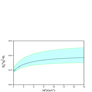
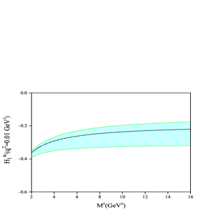
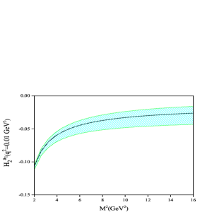
Figure 1: $D^{0}\to a_{1}^{-}$ helicity form factors as functions of $M^{2}$. For $\mathcal{H}_{0}^{a_{1}}$ we take $q^{2}=0$ while, for $\mathcal{H}_{1,2}^{a_{1}}$ the results are plotted at $q^{2}=0.01~{}\rm{GeV}^{2}$. The threshold parameter is taken $s_{0}=(7\pm 0.2)~{}\rm{GeV}^{2}$ for every plot.

The contributions of twist-2 and twist-3 distribution amplitudes and higher states in the $D^{0}\to a_{1}^{-}$ helicity form factors, with respect to $M^{2}$, are displaced in Figs. 2 and 3. It can be observed that at the above-mentioned interval from Borel mass, the higher twist contributions as well as higher states, are suppressed. Our numerical analysis shows, that the contribution of the higher states is smaller than about $8\%$ of the total value.

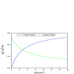
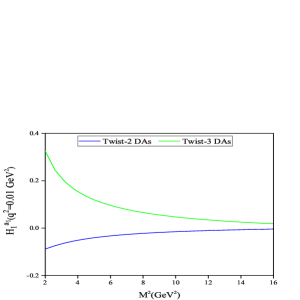
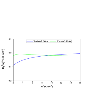
Figure 2: The contributions of twist-2 and twist-3 distribution amplitudes in the $D^{0}\to a_{1}^{-}$ helicity form factors on $M^{2}$ and $s_{0}=7~{}\rm{GeV}^{2}$. The values of $q^{2}$ are taken as Fig. 1.

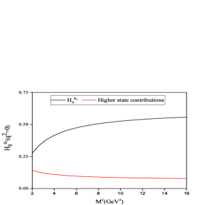
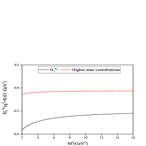
Figure 3: $D^{0}\to a_{1}^{-}$ helicity form factors as a function of $M^{2}$ for $s_{0}=7~{}\rm{GeV}^{2}$ as well as the higher states contributions in these form factors. The values of $q^{2}$ are chosen as Fig. 1.

Using all the input values and parameters, the helicity form factors can be evaluated as a function of $q^{2}$. The values of $\mathcal{H}_{0}$ for aforementioned decays at the zero transferred momentum square $q^{2}=0$ are presented in Table 3. In this table, the contributions of twist-2 distribution amplitudes are also reported. The main uncertainty in ${\mathcal{H}}_{0}(q^{2}=0)$ comes from $c$ quark mass $m_{c}$ and $\Phi_{\perp}$ light cone distribution amplitude.

process	${\mathcal{H}}_{0}(q^{2}=0)$	Twist-2	process	${\mathcal{H}}_{0}(q^{2}=0)$	Twist-2
$D^{0}\to a^{-}_{1}\ell^{+}\nu$	$0.67^{+0.26}_{-0.08}$	$0.56^{+0.21}_{-0.05}$	$D^{0}\to b^{-}_{1}\ell^{+}\nu$	$-0.76^{+0.22}_{-0.19}$	$-0.62^{+0.16}_{-0.10}$
$D^{+}\to a^{0}_{1}\ell^{+}\nu$	$0.46^{+0.18}_{-0.05}$	$0.38^{+0.14}_{-0.03}$	$D^{+}\to b^{0}_{1}\ell^{+}\nu$	$-0.53^{+0.15}_{-0.13}$	$-0.43^{+0.11}_{-0.10}$
$D\to K_{1A}\ell^{+}\nu$	$0.51^{+0.20}_{-0.04}$	$0.40^{+0.15}_{-0.03}$	$D\to K_{1B}\ell^{+}\nu$	$-0.95^{+0.25}_{-0.21}$	$-0.83^{+0.21}_{-0.15}$
$D_{s}\to K_{1A}\ell^{+}\nu$	$0.31^{+0.14}_{-0.12}$	$0.21^{+0.11}_{-0.08}$	$D_{s}\to K_{1B}\ell^{+}\nu$	$-0.40^{+0.15}_{-0.18}$	$-0.32^{+0.11}_{-0.12}$

Table 3: Helicity form factor ${\mathcal{H}}_{0}$ as well as contribution of twist-2 distribution amplitudes of the $D^{+}\to a^{0}_{1}(b^{0}_{1})~{}\ell^{+}\nu$, $D^{0}\to a^{-}_{1}(b^{-}_{1})~{}\ell^{+}\nu$, $D\to K_{1A}(K_{1B})~{}\ell^{+}\nu$ and $D_{s}\to K_{1A}(K_{1B})~{}\ell^{+}\nu$ decays at $q^{2}=0$.

In order to extend LCSR prediction to the whole physical region, $m_{\ell}^{2}\leq q^{2}\leq(m_{D_{(s)}}-m_{A})^{2}$, we use the series expansion given in Bharucha2010 as:

$$\mathcal{H}_{0}^{A}(q^{2}) = \frac{1}{z(q^{2},m_{D_{(s)}^{r}}^{2})\sqrt{z(q^{2},t_{-})}\,\phi(q^{2})}\sum_{k=0,1}a_{k}^{A,0}z^{k}(q^{2},t_{0}),$$ (25)

$$\mathcal{H}_{1}^{A}(q^{2}) = \frac{\sqrt{-z(q^{2},0)}}{z(q^{2},m_{D_{(s)}^{r}}^{2})\,\phi(q^{2})}\sum_{k=0,1}a_{k}^{A,1}z^{k}(q^{2},t_{0}),$$ (26)

$$\mathcal{H}_{2}^{A}(q^{2}) = \frac{\sqrt{-z(q^{2},0)}}{z(q^{2},m_{D_{(s)}^{r}}^{2})\sqrt{z(q^{2},t_{-})}\,\phi(q^{2})}\sum_{k=0,1}a_{k}^{A,2}z^{k}(q^{2},t_{0}),$$ (27)

where

$$z(q^{2},t)=\frac{\sqrt{t_{+}-q^{2}}-\sqrt{t_{+}-t}}{\sqrt{t_{+}-q^{2}}+\sqrt{t_{+}-t}},$$ (28)

$$\sqrt{-z(q^{2},0)}=\sqrt{q^{2}}/m_{D_{(s)}^{r}},$$ (29)

where $t=t_{0},~{}t_{-},~{}m_{D_{(s)}}$ with $t_{\pm}=(m_{D_{(s)}}\pm m_{A})^{2}$ and $t_{0}=t_{+}(1-\sqrt{1-t_{-}/t_{+}})$. Moreover, $D_{(s)}^{r}$ shows the resonance states are given in Table 2. The function $\phi(q^{2})$ is given by Arnesen2005 :

$$\phi(q^{2})=\sqrt{\frac{3t_{+}t_{-}}{32\pi\chi_{0}}}\,\left(\frac{z(q^{2},0)}{-q^{2}}\right)^{2}\,\left(\frac{z(q^{2},t_{0})}{t_{0}-q^{2}}\right)^{-0.5}\,\left(\frac{z(q^{2},t_{-})}{t_{-}-q^{2}}\right)^{-0.25}\,\left(\frac{(t_{+}-q^{2})^{2}}{t_{+}-t_{0}}\right)^{0.25},$$ (30)

where $\chi_{0}$ has been calculated using OPE and is given by Bharucha2010 :

$$\chi_{0}=\frac{1+0.751\alpha_{s}(m_{c})}{8\pi^{2}}$$ (31)

It should be noted that for the functions $\sqrt{z(q^{2},t_{-})}$ and $\phi(q^{2})$ the replacement $m_{D_{(s)}}\to m_{D_{(s)}^{r}}$ must be made. For the series expansion parameterizations 25, 26 and 27, the unitarity constraints are obtained as Bharucha2010 :

$$\sum_{k=0,1}\left\{(a_{k}^{A,0})^{2}+(a_{k}^{A,1})^{2}+(a_{k}^{A,2})^{2}\right\}\leq 1$$ (32)

We use parameter $\Delta$ defined as:

$$\Delta=\frac{\sum_{q^{2}}\left|\mathcal{H}^{A}_{\sigma}(q^{2})-\mathcal{H}^{A,\rm fit}_{\sigma}(q^{2})\right|}{\sum_{q^{2}}\left|\mathcal{H}^{A}_{\sigma}(q^{2})\right|}\times 100,$$ (33)

where $0\leq~{}q^{2}~{}\leq(m_{D_{(s)}}-m_{A})^{2}/2$ to estimate quality of fit for each helicity form factor. Table 4 includes the values of $a_{1}^{\sigma}$, $a_{2}^{\sigma}$ and $\Delta$ for the helicity form factors of the semileptonic decays. For these results all the input parameters are set to be their central values. As it can be seen from the values of $\Delta$ parameters, are reported in 4, the fit functions 25, 26 and 27 cover the LCSR predictions for the helicity form factors.

Table 4: Values of $b_{0}$, $b_{1}$ and $b_{2}$ related to $F^{(1)}(q^{2})$ for the fitted form factors of $D_{(s)}\to a_{1},b_{1},K_{1A}$ and $K_{1B}$ transitions.

Form factor	${a_{1}}$	$a_{2}$	$\Delta$	Form factor	${a_{1}}$	$a_{2}$	$\Delta$
$\mathcal{H}_{0}^{D^{0}\to a^{-}_{1}}$	${0.05}$	$-0.95$	$0.36$	$\mathcal{H}_{0}^{D^{0}\to b^{-}_{1}}$	${-0.10}$	$0.49$	$0.32$
$\mathcal{H}_{1}^{D^{0}\to a^{-}_{1}}$	${-0.07}$	$-0.56$	$0.26$	$\mathcal{H}_{1}^{D^{0}\to b^{-}_{1}}$	${0.12}$	$-0.54$	$0.17$
$\mathcal{H}_{2}^{D^{0}\to a^{-}_{1}}$	${-0.12}$	$0.83$	$0.24$	$\mathcal{H}_{2}^{D^{0}\to b^{-}_{1}}$	${0.10}$	$-0.87$	$0.50$
$\mathcal{H}_{0}^{D^{+}\to a^{0}_{1}}$	${0.03}$	$-0.67$	$0.35$	$\mathcal{H}_{0}^{D^{+}\to b^{0}_{1}}$	${-0.07}$	$0.34$	$0.31$
$\mathcal{H}_{1}^{D^{+}\to a^{0}_{1}}$	${-0.04}$	$-0.39$	$0.26$	$\mathcal{H}_{1}^{D^{+}\to b^{0}_{1}}$	${0.08}$	$-0.38$	$0.16$
$\mathcal{H}_{2}^{D^{+}\to a^{0}_{1}}$	${-0.09}$	$0.59$	$0.24$	$\mathcal{H}_{2}^{D^{+}\to b^{0}_{1}}$	${0.07}$	$-0.61$	$0.48$
$\mathcal{H}_{0}^{D\to K_{1A}}$	${0.12}$	$-0.54$	$0.57$	$\mathcal{H}_{0}^{D\to K_{1B}}$	${-0.04}$	$0.68$	$0.83$
$\mathcal{H}_{1}^{D\to K_{1A}}$	${-0.09}$	$-0.85$	$0.30$	$\mathcal{H}_{1}^{D\to K_{1B}}$	${0.16}$	$-0.71$	$0.57$
$\mathcal{H}_{2}^{D\to K_{1A}}$	${-0.02}$	$0.08$	$0.29$	$\mathcal{H}_{2}^{D\to K_{1B}}$	${0.16}$	$-0.90$	$0.54$
$\mathcal{H}_{0}^{D_{s}\to K_{1A}}$	${0.02}$	$0.85$	$0.17$	$\mathcal{H}_{0}^{D_{s}\to K_{1B}}$	${-0.05}$	$0.72$	$0.22$
$\mathcal{H}_{1}^{D_{s}\to K_{1A}}$	${-0.07}$	$-0.76$	$0.05$	$\mathcal{H}_{1}^{D_{s}\to K_{1B}}$	${0.12}$	$-0.82$	$0.19$
$\mathcal{H}_{2}^{D_{s}\to K_{1A}}$	${-0.01}$	$-0.14$	$0.05$	$\mathcal{H}_{2}^{D_{s}\to K_{1B}}$	${0.04}$	$-0.77$	$0.11$

The dependence of the form factors $\mathcal{H}_{0}$, $\mathcal{H}_{1}$ and $\mathcal{H}_{2}$ for $D^{0}\to a^{-}_{1}$ and $D^{0}\to b^{-}_{1}$ transitions on $q^{2}$ are plotted in Fig. 4. In these plots, the LCSR results and the fitted form factors are displaced with circles and black lines, respectively. Moreover, the shaded regions are obtained using upper and lower values of the input parameters.

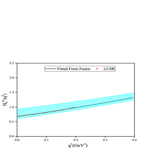
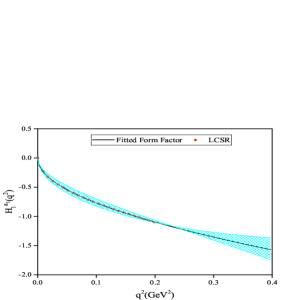
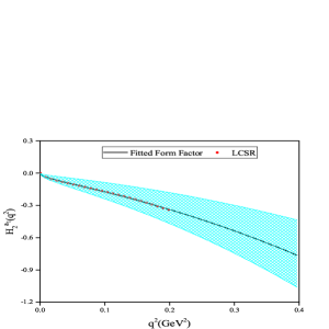
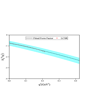
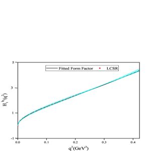
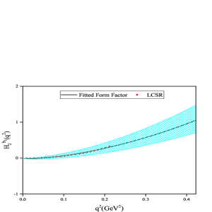
Figure 4: $D^{0}\to a_{1}^{-}$ and $D^{0}\to b_{1}^{-}$ helicity form factors as a function of $q^{2}$. Circles show the results of the LCSR while, black lines show the fitted form factors in the whole physical regions. The shaded bands stand for the results correspond the upper and lower values of the input parameters.

III.2 Analysis of the branching ratios

Now, we are ready to estimate the branching ratio values for the semileptonic $D_{(s)}\to A\ell\nu$ decays. The differential decay width of considered semileptonic decays is evaluated in SM as:

$$\frac{d\Gamma(D_{(s)}\rightarrow A\ell\nu)}{dq^{2}}=\frac{{\sqrt{\lambda}}\,G_{F}^{2}\,\left|V_{cq^{\prime}}\right|^{2}}{192\,\pi^{3}\,m_{D_{(s)}}^{3}}\Bigg{\{}[\mathcal{H}^{A}_{0}(q^{2})]^{2}+[\mathcal{H}^{A}_{1}(q^{2})]^{2}+[\mathcal{H}^{A}_{2}(q^{2})]^{2}\Bigg{\}},$$ (34)

where $V_{cq^{\prime}}=V_{cd}(V_{cs})$ is used for $c\to d(s)\,\ell\nu$ transition. To calculate the branching ratios, the total mean life time $\tau_{D^{0}}=0.41$, $\tau_{D^{+}}=1.04$ and $\tau_{D^{+}_{s}}=0.50$ ps pdg are used for the $D_{(s)}$ states. The differential branching ratios of $D^{0}\to a^{-}_{1}(b^{-}_{1})\ell\nu$ with their uncertainly regions, are plotted with respect to $q^{2}$ in Fig. 5. Moreover, our results for the branching ratio values of the semileptonic decays $D^{0}\to a_{1}^{-}(b_{1}^{-})\ell\nu$ and $D^{+}\to a^{0}_{1}(b^{0}_{1})\ell\nu$ decays as well as the estimations of the other approaches are presented in Fig. 6. The predictions of LCSR, 3PSR and CLFQM are calculated by using transition form factors.

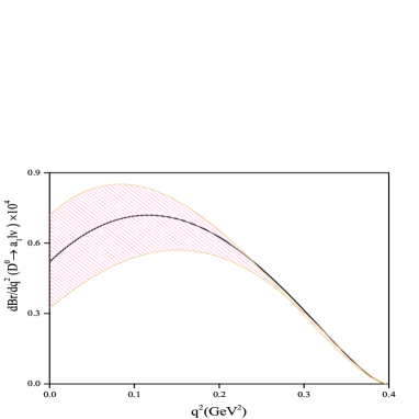
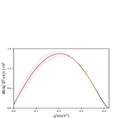
Figure 5: The differential branching ratio of $D^{0}\to a_{1}^{-}$ and $D^{0}\to b_{1}^{-}$ decays as a function of $q^{2}$. The shaded intervals show the results obtained using the upper and lower values of the input parameters.

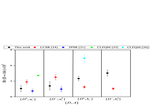
Figure 6: Our predictions for branching ratio values of the semileptonic $D^{0}\to a_{1}^{-}(b_{1}^{-})\ell\nu$ and $D^{+}\to a^{0}_{1}(b^{0}_{1})\ell\nu$ decays. The results of the other methods, estimated using transition form factors, such as LCSR, 3PSR and CLFQM are also reported.

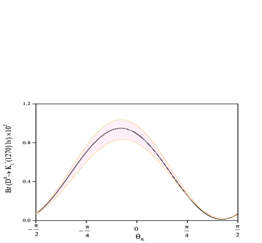
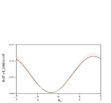
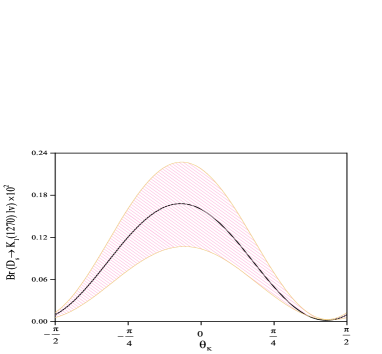
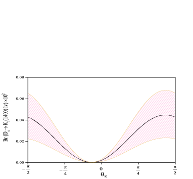
Figure 7: The $\theta_{K}$ dependence of differential branching ratios of the semileptonic $D_{(s)}\to K_{1}(1270)\ell\nu$ and $D_{(s)}\to K_{1}(1400)\ell\nu$ transitions with their uncertainly bands.

The $\theta_{K}$ dependence of the branching ratio values of $D_{(s)}$ decays into the physical states $K_{1}(1270)$ and $K_{1}(1400)$, are displaced in Fig. 7; and comparison between our results and other theoretical technics at $\theta_{K}={-(34\pm 13)}^{\circ}$ are given in Fig. 8. The $D^{+}\to K_{1}^{0}(1270)~{}e^{+}\nu_{e}$ decay is searched at the BEPCII collider and its decay branching fraction is determined to be $\mathcal{B}(D^{+}\to K_{1}^{0}(1270)~{}e^{+}\nu_{e})=(2.30\pm 0.69)$ Ablikim2019 . Our branching ratio of $D^{+}\to K_{1}^{0}(1270)~{}e^{+}\nu_{e}$ agrees with the experimental measurement when $\theta_{K}=-(36.68\pm 6.30)^{\circ}$.

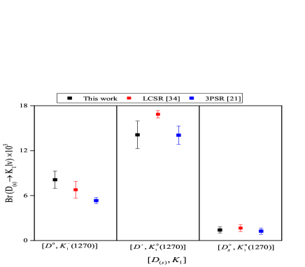
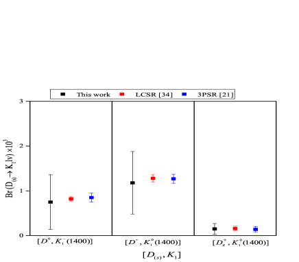
Figure 8: Theatrical values for the branching ratio of the semileptonic $D_{(s)}\to K_{1}$ with $K_{1}=K_{1}(1270),K_{1}(1400)$ at $\theta_{K}={-(34\pm 13)}^{\circ}$.

In summary, we calculate the $D_{(s)}$ to axial vector mesons $a_{1}^{-}$, $a_{1}^{0}$, $b_{1}^{-}$, $b_{1}^{0}$, $K_{1}(1270)$ and $K_{1}(1400)$ helicity form factors using the light cone QCD sum rules. The uncertainties of the helicity form factors come from the borel parameter $M^{2}$, the charm quark mass $m_{c}$ and $\Phi_{\perp}$ twist-2 light cone distribution amplitude of the axial vector meson. To extend the LCSR calculations to the full physical region, the extrapolated series expansions are used and the low-lying $D$ meson resonances with ${1}^{+}$ and $1^{-}$ quantum numbers were utilized as the dominant poles. Based on the fitted form factors, predictions for the branching ratios of relevant semileptonic decays were reported and a comparison was made between our results and other method estimations. Our calculation for branching ratio of $D^{+}\to K_{1}^{0}(1270)~{}e^{+}\nu_{e}$ decay is in good agreement with the BEPCII collider measurement within errors at the mixing angle $\theta_{k}=-(36.68\pm 6.30)^{\circ}$

Appendix: Twist Function Definitions

In this appendix, we present the definitions for the two–parton LCDAs as well as the twist functions. Two–particle chiral–even distribution amplitudes are given by Kwei :

$$\langle 0|\bar{q}_{\alpha}(x)\,q_{\delta}(0)|A(p,\varepsilon)\rangle = -\frac{i}{4}\int_{0}^{1}du~{}e^{-iup^{\prime}.x}\Bigg{\{}f_{A}m_{A}\Bigg{[}\not\!p\gamma_{5}\frac{\varepsilon.x}{p.x}\Phi_{\parallel}(u)+\Bigg{(}\not\!\varepsilon-\not\!p\frac{\varepsilon.x}{p.x}\Bigg{)}\gamma_{5}g_{\perp}^{(a)}(u)$$ (35)

$$- \not\!x\gamma_{5}\frac{\varepsilon.x}{2(p.x)^{2}}m_{A}^{2}\phi_{b}(u)+\epsilon_{\mu\nu\rho\sigma}\varepsilon^{\nu}p^{\rho}x^{\sigma}\gamma^{\mu}\frac{g_{\perp}^{(v)}(u)}{4}\Bigg{]}$$

$$+ \,f^{\perp}_{A}\Bigg{[}\frac{1}{2}(\not\!p\not\!\epsilon-\not\!\epsilon\not\!p)\gamma_{5}\,\Phi_{\perp}(u)-\frac{1}{2}(\not\!p\not\!x-\not\!x\not\!p)\gamma_{5}\frac{\epsilon.x}{(p.x)^{2}}m_{A}^{2}\bar{h}_{\parallel}^{(t)}(u)$$

$$+ i\Big{(}\epsilon.x\Big{)}m_{A}^{2}\gamma_{5}\frac{h^{(p)}_{\parallel}(u)}{2}\Bigg{]}\Bigg{\}}_{\delta\alpha},$$

$$\langle 0|\bar{q}(x)\gamma_{\mu}\gamma_{5}q^{\prime}(0)|A(p,\varepsilon)\rangle = if_{A}m_{A}\int_{0}^{1}du\,e^{-iup.x}\Bigg{\{}p_{\mu}\frac{\varepsilon.x}{p.x}\Phi_{\parallel}(u)+\left(\varepsilon_{\mu}-p_{\mu}\frac{\varepsilon.x}{p.x}\right)g_{\perp}^{(a)}(u)+{\cal O}(x^{2})\Bigg{\}}~{},$$

$$\langle 0|\bar{q}(x)\gamma_{\mu}q^{\prime}(0)|A(p,\varepsilon)\rangle = -if_{A}\,m_{A}~{}\epsilon_{\mu\nu\rho\sigma}\varepsilon^{\nu}p^{\rho}x^{\sigma}\int_{0}^{1}du\,e^{-iu\,p.x}\Bigg{\{}\frac{g_{\perp}^{(v)}(u)}{4}+{\cal O}(x^{2})\Bigg{\}},$$ (36)

also, two–particle chiral–odd distribution amplitudes are defined by:

$$\langle 0|\bar{q}(x)\sigma_{\mu\nu}\gamma_{5}q^{\prime}(0)|A(p,\varepsilon)\rangle = f_{A}^{\perp}\int_{0}^{1}du\,e^{-iup^{\prime}.x}\Bigg{\{}(\varepsilon_{\mu}p_{\nu}-\varepsilon_{\nu}p_{\mu})\Phi_{\perp}(u)+\frac{{m^{2}_{A}}\,\varepsilon.x}{(p.x)^{2}}(p_{\mu}x_{\nu}-p_{\nu}x_{\mu})\bar{h}_{\parallel}^{(t)}+{\cal O}(x^{2})\Bigg{\}},$$

$$\langle 0|\bar{q}(x)\gamma_{5}q^{\prime}(0)|A(p,\varepsilon)\rangle = f_{A}^{\perp}m_{A}^{2}(\varepsilon.x)\int_{0}^{1}du\,e^{-iup.x}\Bigg{\{}\frac{h_{\parallel}^{(p)}(u)}{2}+{\cal O}(x^{2})\Bigg{\}}.$$ (37)

In these expressions, $f_{A}$ and $f_{A}^{\perp}$ are decay constants of the axial vector meson $A$. We set $f_{A}^{\perp}=f_{A}$ in $\mu=1~{}{\rm GeV}$, such that we have

$$\langle 0|\bar{q}(0)\sigma_{\mu\nu}\gamma_{5}q^{\prime}(0)|A(p,\varepsilon)\rangle=a_{0}^{A}\,f_{A}\,(\epsilon_{\mu}p_{\nu}-\epsilon_{\nu}p_{\mu}),$$ (38)

where $a_{0}^{\perp}$ refers to the zeroth Gegenbauer moments of $\Phi_{\perp}$. It should be noted that $f_{A}$ is scale–independent and conserves $G$-parity, but $f_{A}^{\perp}$ is scale–dependent and violates $G$-parity.

We take into account the approximate forms of twist-2 distributions for the $A=a_{1},K_{1A}$ states to be Kwei2

$$\Phi_{\parallel}(u) = 6u\bar{u}\left[1+3a_{1}^{\parallel}\,\xi+a_{2}^{\parallel}\,\frac{3}{2}(5\xi^{2}-1)\right],$$ (39)

$$\Phi_{\perp}(u) = 6u\bar{u}\left[a_{0}^{\perp}+3a_{1}^{\perp}\,\xi+a_{2}^{\perp}\,\frac{3}{2}(5\xi^{2}-1)\right],$$ (40)

and for the $A=b_{1},K_{1B}$ to be

$$\Phi_{\parallel}(u) = 6u\bar{u}\left[a_{0}^{\parallel}+3a_{1}^{\parallel}\,\xi+a_{2}^{\parallel}\,\frac{3}{2}(5\xi^{2}-1)\right],$$ (41)

$$\Phi_{\perp}(u) = 6u\bar{u}\left[1+3a_{1}^{\perp}\,\xi+a_{2}^{\perp}\,\frac{3}{2}(5\xi^{2}-1)\right],$$ (42)

where $\xi=2u-1$.

For the relevant two-parton twist-3 chiral-even LCDAs, we take the approximate expressions up to conformal spin $9/2$ and ${\cal O}(m_{s})$ Kwei2 :

$$g_{\perp}^{(a)}(u) = \frac{3}{4}(1+\xi^{2})+\frac{3}{2}\,a_{1}^{\parallel}\,\xi^{3}+\left(\frac{3}{7}\,a_{2}^{\parallel}+5\zeta_{3,A}^{V}\right)\left(3\xi^{2}-1\right)$$ (43)

$${}+\left(\frac{9}{112}\,a_{2}^{\parallel}+\frac{105}{16}\,\zeta_{3,A}^{A}-\frac{15}{64}\,\zeta_{3,A}^{V}\omega_{A}^{V}\right)\left(35\xi^{4}-30\xi^{2}+3\right)$$

$$+5\Bigg{[}\frac{21}{4}\zeta_{3,A}^{V}\sigma_{A}^{V}+\zeta_{3,A}^{A}\bigg{(}\lambda_{A}^{A}-\frac{3}{16}\sigma_{A}^{A}\Bigg{)}\Bigg{]}\xi(5\xi^{2}-3)$$

$${}-\frac{9}{2}\bar{a}_{1}^{\perp}\,\widetilde{\delta}_{+}\,\left(\frac{3}{2}+\frac{3}{2}\xi^{2}+\ln u+\ln\bar{u}\right)-\frac{9}{2}\bar{a}_{1}^{\perp}\,\widetilde{\delta}_{-}\,(3\xi+\ln\bar{u}-\ln u),$$

$$g_{\perp}^{(v)}(u) = 6u\bar{u}\Bigg{\{}1+\Bigg{(}a_{1}^{\parallel}+\frac{20}{3}\zeta_{3,A}^{A}\lambda_{A}^{A}\Bigg{)}\xi$$ (44)

$$+\Bigg{[}\frac{1}{4}a_{2}^{\parallel}+\frac{5}{3}\,\zeta^{V}_{3,A}\left(1-\frac{3}{16}\,\omega^{V}_{A}\right)+\frac{35}{4}\zeta^{A}_{3,A}\Bigg{]}(5\xi^{2}-1)$$

$$+\frac{35}{4}\Bigg{(}\zeta_{3,A}^{V}\sigma_{A}^{V}-\frac{1}{28}\zeta_{3,A}^{A}\sigma_{A}^{A}\Bigg{)}\xi(7\xi^{2}-3)\Bigg{\}}$$

$${}-18\,\bar{a}_{1}^{\perp}\widetilde{\delta}_{+}\,(3u\bar{u}+\bar{u}\ln\bar{u}+u\ln u)-18\,\bar{a}_{1}^{\perp}\widetilde{\delta}_{-}\,(u\bar{u}\xi+\bar{u}\ln\bar{u}-u\ln u),$$

$$h_{\parallel}^{(t)}(u) = 3a_{0}^{\perp}\xi^{2}+\frac{3}{2}\,a_{1}^{\perp}\,\xi(3\xi^{2}-1)+\frac{3}{2}\Bigg{[}a_{2}^{\perp}\xi+\zeta^{\perp}_{3,A}\Bigg{(}5-\frac{\omega_{A}^{\perp}}{2}\Bigg{)}\Bigg{]}\,\xi\,(5\xi^{2}-3)$$ (45)

$$+\frac{35}{4}\zeta^{\perp}_{3,A}\sigma^{\perp}_{A}(35\xi^{4}-30\xi^{2}+3)+18\bar{a}_{2}^{\parallel}\Bigg{[}\delta_{+}\xi-\frac{5}{8}\delta_{-}(3\xi^{2}-1)\Bigg{]}$$

$$-\frac{3}{2}\,\Bigg{(}\delta_{+}\,\xi[2+\ln(\bar{u}u)]+\,\delta_{-}\,[1+\xi\ln(\bar{u}/u)]\Bigg{)}(1+6\bar{a}_{2}^{\parallel}),$$

$$h_{\parallel}^{(p)}(u) = 6u\bar{u}\Bigg{\{}a_{0}^{\perp}+\Bigg{[}a_{1}^{\perp}+5\zeta^{\perp}_{3,A}\Bigg{(}1-\frac{1}{40}(7\xi^{2}-3)\omega_{A}^{\perp}\Bigg{)}\Bigg{]}\xi$$ (46)

$$\ \ \ \ \ \ \ +\Bigg{(}\frac{1}{4}a_{2}^{\perp}+\frac{35}{6}\zeta^{\perp}_{3,A}\sigma^{\perp}_{A}\Bigg{)}(5\xi^{2}-1)-5\bar{a}_{2}^{\parallel}\Bigg{[}\delta_{+}\xi+\frac{3}{2}\delta_{-}(1-\bar{u}u)\Bigg{]}\Bigg{\}}$$

$${}-3[\,\delta_{+}\,(\bar{u}\ln\bar{u}-u\ln u)+\,\delta_{-}\,(u\bar{u}+\bar{u}\ln\bar{u}+u\ln u)](1+6\bar{a}_{2}^{\parallel}),$$

for $A=a_{1},K_{1A}$ states, and

$$g_{\perp}^{(a)}(u) = \frac{3}{4}a_{0}^{\parallel}(1+\xi^{2})+\frac{3}{2}\,a_{1}^{\parallel}\,\xi^{3}+5\left[\frac{21}{4}\,\zeta_{3,A}^{V}+\zeta_{3,A}^{A}\Bigg{(}1-\frac{3}{16}\omega_{A}^{A}\Bigg{)}\right]\xi\left(5\xi^{2}-3\right)$$ (47)

$${}+\frac{3}{16}\,a_{2}^{\parallel}\left(15\xi^{4}-6\xi^{2}-1\right)+5\,\zeta^{V}_{3,A}\lambda^{V}_{A}\left(3\xi^{2}-1\right)$$

$${}+\frac{105}{16}\left(\zeta^{A}_{3,A}\sigma^{A}_{A}-\frac{1}{28}\zeta^{V}_{A}\sigma^{V}_{A}\right)\left(35\xi^{4}-30\xi^{2}+3\right)$$

$${}-15\bar{a}_{2}^{\perp}\bigg{[}\widetilde{\delta}_{+}\xi^{3}+\frac{1}{2}\widetilde{\delta}_{-}(3\xi^{2}-1)\bigg{]}$$

$${}-\frac{3}{2}\,\bigg{[}\widetilde{\delta}_{+}\,(2\xi+\ln\bar{u}-\ln u)+\,\widetilde{\delta}_{-}\,(2+\ln u+\ln\bar{u})\bigg{]}(1+6\bar{a}_{2}^{\perp}),$$

$$g_{\perp}^{(v)}(u) = 6u\bar{u}\Bigg{\{}a_{0}^{\parallel}+a_{1}^{\parallel}\xi+\Bigg{[}\frac{1}{4}a_{2}^{\parallel}+\frac{5}{3}\zeta^{V}_{3,A}\Bigg{(}\lambda^{V}_{A}-\frac{3}{16}\sigma^{V}_{A}\Bigg{)}+\frac{35}{4}\zeta^{A}_{3,A}\sigma^{A}_{A}\Bigg{]}(5\xi^{2}-1)$$ (48)

$${}+\frac{20}{3}\,\xi\left[\zeta^{A}_{3,A}+\frac{21}{16}\Bigg{(}\zeta^{V}_{3,A}-\frac{1}{28}\,\zeta^{A}_{3,A}\omega^{A}_{A}\Bigg{)}(7\xi^{2}-3)\right]$$

$${}-5\,\bar{a}_{2}^{\perp}[2\widetilde{\delta}_{+}\xi+\widetilde{\delta}_{-}(1+\xi^{2})]\Bigg{\}}$$

$${}-6\bigg{[}\,\widetilde{\delta}_{+}\,(\bar{u}\ln\bar{u}-u\ln u)+\,\widetilde{\delta}_{-}\,(2u\bar{u}+\bar{u}\ln\bar{u}+u\ln u)\bigg{]}(1+6\bar{a}_{2}^{\perp}),$$

$$h_{\parallel}^{(t)}(u) = 3\xi^{2}+\frac{3}{2}\,a_{1}^{\perp}\,\xi(3\xi^{2}-1)+\Bigg{[}\frac{3}{2}a_{2}^{\perp}\,\xi+\frac{15}{2}\zeta^{\perp}_{3,A}\Bigg{(}\lambda^{\perp}_{A}-\frac{1}{10}\sigma^{\perp}_{A}\Bigg{)}\Bigg{]}\,\xi(5\xi^{2}-3)$$ (49)

$${}+\frac{35}{4}\zeta^{\perp}_{3,A}(35\xi^{4}-30\xi^{2}+3)$$

$${}+\frac{9}{2}\bar{a}_{1}^{\parallel}\,\xi\Bigg{[}\delta_{+}\,(\ln u-\ln\bar{u}-3\xi)-\delta_{-}\,\Bigg{(}\ln u+\ln\bar{u}+\frac{8}{3}\Bigg{)}\Bigg{]}\,,$$

$$h_{\parallel}^{(p)}(u) = 6u\bar{u}\Bigg{\{}1+a_{1}^{\perp}\xi+\left(\frac{1}{4}a_{2}^{\perp}+\frac{35}{6}\,\zeta^{\perp}_{3,A}\right)(5\xi^{2}-1)$$ (50)

$${}+5\zeta^{\perp}_{3,A}\Bigg{[}\lambda^{\perp}_{A}-\frac{1}{40}(7\xi^{3}-3)\sigma^{\perp}_{A}\Bigg{]}\,\xi\Bigg{\}}$$

$${}-9\bar{a}_{1}^{\parallel}\,\delta_{+}\,(3u\bar{u}+\bar{u}\ln\bar{u}+u\ln u)-9\bar{a}_{1}^{\parallel}\,\delta_{-}\,\Bigg{(}\frac{2}{3}\xi u\bar{u}+\bar{u}\ln\bar{u}-u\ln u\Bigg{)}\,,$$

for $A=b_{1},K_{1B}$ states. where

$$\widetilde{\delta}_{\pm}={f_{A}^{\perp}\over f_{A}}{m_{q_{2}}\pm m_{q_{1}}\over m_{A}},\qquad\zeta_{3,A}^{V(A)}=\frac{f^{V(A)}_{3A}}{f_{A}m_{A}}.$$ (51)

References

(1)
M. Artuso, B. Meadows and A. A. Petrov, Ann. Rev. Nucl. Part. Sci
58, 249 (2008).
(2)
T. Feldmann, B. Mueller and D. Seidel, JHEP 1708, 105 (2017).
(3)
J. Zhang, C. X. Yue, C. H. Li, Eur. Phys. J. C 78, 695 (2018).
(4)
A. Khodjamirian, R. Ruckl, S. Weinzierl, C. Winhart, and O. I. Yakovlev, Phys.Rev. D 62,
114002 (2000).
(5)
P. Ball, Phys. Lett. B 641, 50 (2006).
(6)
H. B. Fu, X. Yang, R. Lu, L. Zeng, W. Cheng and X. G. Wu,
arXiv:1808.06412 [hep-ph].
(7)
N. R. Soni and J. N. Pandya, Phys. Rev. D 96, 016017 (2017).
(8)
N. R. Soni, M. A. Ivanov, J. G. Korner, J. N. Pandya, P. Santorelli
and C. T. Tran, arXiv:1810.11907 [hep-ph].
(9)
W. Y. Wang, Y. L. Wu, and M. Zhong, Phys. Rev. D 67, 014024 (2003).
(10)
A. Abada et al. (SPQcdR collaboration), Nucl. Phys. Proc. Suppl. 119, 625 (2003).
(11)
C. Aubin et al. (Fermilab Lattice), Phys. Rev. Lett. 94, 011601 (2005).
(12)
C. Bernard et al., Phys. Rev. D 80, 034026 (2009).
(13)
I. Bediaga and M. Nielsen, Phys. Rev. D 68, 036001 (2003).
(14)
T. M. Aliev, V. L. Eletsky, and Ya. I. Kogan, Sov. J. Nucl. Phys.
40, 527 (1984).
(15)
P. Ball, V. M. Braun, and H. G. Dosch, Phys. Rev. D 44, 3567
(1991).
(16)
P. Ball, Phys. Rev. D 48, 3190 (1993).
(17)
A. A. Ovchinnikov and V. A. Slobodenyuk, Z. Phys. C 44, 433
(1989); V. N. Baier and A. Grozin, Z. Phys. C 47, 669 (1990).
(18)
D. S. Du, J. W. Li, and M. Z. Yang, Eur. Phys. J. C 37, 137
(2004).
(19)
M. Z. Yang, Phys. Rev. D 73, 034027 (2006); 73,
079901(E) (2006).
(20)
R. Khosravi, K. Azizi and N. Ghahramany, Phys. Rev. D 79,
036004 (2009).
(21)
Y. Zuo et al, Int. J. Mod. Phys. A 31, 1650116 (2016).
(22)
A. Bharucha, T. Feldmann and M. Wick, JHEP 1009, 090 (2010).
(23)
W. A. Bardeen, E. J. Eichten, and C. T. Hill, Phys. Rev. D 68, 054024 (2003).
(24)
C. Patrignani et al. (Particle Data Group), Chin. Phys. C 40,
100001 (2016).
(25)
W. Cheng, X. G. Wu, R. Y. Zhou and H. B. Fu, Phys. Rev. D 98, 096013 (2018).
(26)
K. Yang, Nucl. Phys. B 776, 187 (2007).
(27)
L. Burakovsky and T. Goldman, Phys. Rev. D 57, 2879 (1998).
(28)
M. Suzuki, Phys. Rev. D 47, 1252 (1993).
(29)
H. Y. Cheng, Phys. Rev. D 67, 094007 (2003).
(30)
H. Hatanaka, K. C. Yang, Phys. Rev. D 77, 094023 (2008).
(31)
K. Yang, Phys. Rev. D 78, 034018 (2008).
(32)
H. Mutuk, Adv. Energy Phys,2018, 8095653 (2018).
(33)
M. C. Arnesen, B. Grinstein, I. Z. Rothstein, and I. W. Stewart, Phys. Rev. Lett., 95, 071802 (2005).
(34)
S. Momeni and R. Khosravi, J . Phys . G 46, 105006 (2019).
(35)
W. Wang and Z. X. Zhao, Eur. Phys. J. C 76, 59 (2016).
(36)
H. Y. Cheng and X. W. Kang, Eur. Phys. J. C 77, 369 (2017); Eur. Phys. J. C 77, 863 (E) (2017).
(37)
M. Ablikim et al. [BESIII Collaboration], arXiv: 1907.11370 [hep-ex].