Strong consistency of the nonparametric local linear regression estimation under censorship model

F. Bouhadjera

Université Badji-Mokhtar, Lab. de Probabilités et Statistique. BP 12, Annaba, 23000, Algérie.

ferielbouhadjera@gmail.com

E. Ould Saïd

Université du Littoral Côte d’Opale, Lab. de Math. Pures et Appliquées, IUT de Calais. 19, rue Louis David. Calais, 62228, France

elias.ould-said@univ-littoral.fr

M. R. Remita

Université Badji-Mokhtar, Lab. de Probabilités et Statistique. BP 12, Annaba, 23000, Algérie.

medriad.remita@univ-annaba.dz

Abstract: We introduce and study a local linear nonparametric regression estimator for censorship model. The main goal of this paper is, to establish the uniform almost sure consistency result with rate over a compact set for the new estimate. To support our theoretical result, a simulation study has been done to make comparison with the classical regression estimator.

Key Words: censored data; local linear estimation; rate of consistency; regression function; survival analysis; uniform almost sure consistency.

1 Introduction

Nonparametric regression is a smoothing method for recovering a regression function from data, which has no restriction on its form. In this context, the modelization of the relationship between two random variables has been studied by many researchers in complete and incomplete data. The most used approaches are kernel methods (see e.g: Guessoum and Ould Saïd (2008)). It is well known that the local linear smoothing procedure has many desirable advantages, for an extensive discussion for what regards the bias and boundary effects in theses issues, we can refer to Fan (1992), Fan and Gijbels (1996) for univariate case and Fan and Yao (2003) for the multivariate case.
In this work, we deal with the problem of the estimation of the regression function under right censorship by using the local linear approach. In this framework, we define a local linear regression estimator by taking in account the synthetic data and establish the uniform almost sure consistency with rate of the resulting estimator. Among the studies dedicated to local linear fit in the case of censored data and without pretending to exhaustivity, we quote Cai (2003) who proposed an estimator of the regression function based on the generalization of the weighted least squares method. We point out that his study does penalize the censoring survival function. Recall that Fan and Gijbels (1994) established the consistency in probability of analogous estimator. Finally, inspired by the works of Beran (1981) and Dabrowska (1987), Kim (1998) used the conditional hazard estimator to define a linear local estimator. We point out that the only result in this framework is the consistency in probability and as far as we know our result is new.
The organization of the article is as follows. In the next section, we give a brief description of nonparametric regression estimates and the proposed methodology. In Section 3, we provide the hypotheses, main results and a sketch of the proof. A comparative study with the classical kernel estimator with different sizes and censoring rates have been done in Section 4. Finally, the proofs are postponed to the Section 5.

2 Model and estimators

Consider $n$ independent and identically distributed replications of a couple $(X_{i},Z_{i})$ having the same distribution as the pair $(X,Z)$ where $Z$ is the interest random variable (r.v.) with unknown distribution function $H$ and $X$ is the corresponding covariate. Under this setting, the purpose of this paper is to consider a regression model $Z=\mu(X)+\varepsilon$ with

$$\mu(x)=\mathbb{E}[Z|X=x]=\frac{\displaystyle\int_{\mathbb{R}}z\;f(z,x)\;dz}{f(x)}=:\frac{S_{0}(x)}{f(x)}$$

where $f(\cdot,\cdot)$, $f(\cdot)$ are the joint density of $(X,Z)$ and marginal density of $X$ respectively and the white noise $\varepsilon$ is assumed to be normally distributed with zero mean and variance $\sigma_{\varepsilon}^{2}$. In the situation of censored data, we do not observe $Z$ but only $Y=\min(Z,C)$ and $\delta=\mathds{1}_{\{Z\leq C\}}$ where $C$ is the censoring variable. In what follows we assume that $Z$ and $C$ are independent. This assumption is required to ensure the identifiability of the model. Under this setting, we consider a specific transformation of the data that take into account the effect of the censoring in the distribution: the so-called synthetic data introduced by Carbonez et al. (1995) and used by Kohler et al.(2002), Guessoum and Ould Saïd (2008) and a large number of authors given, for $1\leq i\leq n$, by

$$Z^{\star}_{i}=\frac{\delta_{i}Y_{i}}{\overline{G}(Y_{i})}.$$ (1)

where $\overline{G}(\cdot)$ denotes the survival function of $C$. In what follows, it is assumed that:

$$(Z_{i},X_{i})_{i}\;\;\text{and}\;\;(C_{i})_{i}\;\;\text{are independent.}$$ (2)

Using the conditional expectation properties and the condition (2), then for all fixed $x$, we have

$$\mathbb{E}[Z^{\star}_{1}|X_{1}=x] =\mathbb{E}\left[\frac{\delta_{1}Y_{1}}{\overline{G}(Y_{1})}\big{|}X_{1}=x\right]$$

$$=\mathbb{E}\left[\mathbb{E}\left[\frac{\mathds{1}_{\{Z_{1}\leq C_{1}\}}Z_{1}}{\overline{G}(Z_{1})}\big{|}Z_{1}\right]\big{|}X_{1}=x\right]$$

$$=\mathbb{E}\left[\frac{Z_{1}}{\overline{G}(Z_{1})}\mathbb{E}\left[\mathds{1}_{\{Z_{1}\leq C_{1}\}}|Z_{1}\right]X_{1}=x\right]$$

$$=\mathbb{E}[Z_{1}|X_{1}=x].$$

Now, assume that the second derivative of $\mu(x)$ exists. Based on the approximation of $\mu(X)\approx\mu(x)+\mu^{\prime}(x)(X-x)\equiv\alpha+\beta(X-x)$ in a neighborhood of a point $x$, we extend the LLR estimator to the censoring case by substituting $Z$ by $Z^{\star}$. The problem of estimating $\mu(x)$ becomes minimizing

$$\arg\min_{\alpha,\beta}\sum_{1\leq i\leq n}\left(Z^{\star}_{i}-\alpha-\beta(X_{i}-x)\right)^{2}K_{i},$$ (3)

with $K_{i}=K\left(h^{-1}(X_{i}-x)\right)$ for all $i=1,\dots,n$ where $K$ is a kernel density, and $h:=h_{n}$ is a sequence of the the strictly positive numbers which goes to zero as $n$ goes to infinity. By a simple algebra computation, solving (3) yields to the ”Pseudo-estimator” defined by

$$\widetilde{\mu}(x)=\frac{\displaystyle\sum_{1\leq i,j\leq n}w_{i,j}(x)Z^{\star}_{j}}{\displaystyle\sum_{1\leq i,j\leq n}w_{i,j}(x)}=:\frac{\widetilde{\mu}_{1}(x)}{\widehat{\mu}_{0}(x)}$$ (4)

where

$$w_{i,j}(x)=(X_{i}-x)\left((X_{i}-x)-(X_{j}-x)\right)K_{i}K_{j}.$$

Of course in data analysis, the survival function $\overline{G}(\cdot)$ is unknown and needs to be estimated. This can be done via the Kaplan and Meier (1958) as an estimator of $\overline{G}$ given by

$$\overline{G}_{n}(t)=\left\{\begin{array}[]{cl}\displaystyle\prod_{i=1}^{n}{\left(1-\frac{1-\delta_{i}}{n-i+1}\right)}^{\mathds{1}_{\{Y_{i}\leq t\}}}&\quad\text{if}\quad t<Y_{(n)},\\ 0&\quad\text{otherwise}\end{array}\right.$$ (5)

where $Y_{(1)}\leq Y_{(2)}\leq\dots\leq Y_{(n)}$ are the order statistics of the $Y_{i}$ and $\delta_{i}$ is a concomitant of $Y_{i}$. The properties of $\overline{G}_{n}(t)$ have been studied by many authors. Hence to get a feasible estimator, we replace (5) in (1), then we get

$$\widehat{Z}^{\star}_{i}=\frac{\delta_{i}Y_{i}}{\overline{G}_{n}(Y_{i})}\quad\quad\text{for}\quad 1\leq i\leq n,$$ (6)

and substituting (6) in (4) we get

$$\widehat{\mu}(x)=\frac{\displaystyle\sum_{1\leq i,j\leq n}w_{i,j}(x)\widehat{Z}^{\star}_{j}}{\displaystyle\sum_{1\leq i,j\leq n}w_{i,j}(x)}=:\frac{\widehat{\mu}_{1}(x)}{\widehat{\mu}_{0}(x)},\quad\quad\quad\left(\frac{0}{0}=:0\right).$$ (7)

The estimator $\widehat{\mu}(\cdot)$ is called the local linear regression (LLR) smoother and it has many desirable statistical properties such as avoiding the edge effects (see:  Fan (1992)).

Remark 1

If $\beta=0$, we obtain the classical regression (CR) estimator given in Guessoum and Ould Saïd (2008) and defined by

$$\mu_{n}(x)=\frac{\displaystyle\sum_{1\leq j\leq n}\widehat{Z}^{\star}_{j}K_{j}}{\displaystyle\sum_{1\leq j\leq n}K_{j}}$$ (8)

3 Assumptions and Main results

Let ${\mathscr{C}}_{0}=\left\{x\in\mathbb{R}/f(x)>0\right\}$ and ${\mathscr{C}}$ be a compact subset of ${\mathscr{C}}_{0}$. Throughout the paper, we assume that for any d.f. $Q$, we have $\tau_{Q}=\sup\{x,Q(x)<1\}$ the upper endpoint of the support. We assume that $\tau_{H}>0$ and $0<\overline{G}(\tau_{H})<\infty$.
When no confusion is possible, we denote by $C$ any generic positive constant. Furthermore, as $Z$ is a lifetime it can be supposed to be bounded. Our assumptions are gathered together for easy references.

• The bandwidth $h$ satisfies $\displaystyle\lim_{n\rightarrow\infty}h=0,\quad\lim_{n\rightarrow\infty}nh=+\infty,\quad\lim_{n\rightarrow\infty}\frac{\log n}{nh}=0$.

• The kernel $K(\cdot)$ is a bounded, symmetric nonnegative function on $\mathscr{C}$.

• The density function $f(\cdot)$ is continuously differentiable and $\displaystyle\sup_{x\in\mathscr{C}}|f^{\prime}(x)|<+\infty$.

• The function $S_{0}(x)$ is continuously differentiable and $\displaystyle\sup_{x\in\mathscr{C}}|S_{0}^{\prime}(x)|<+\infty$.

• The function $\upsilon_{k}(x)=\int z^{k}f_{Z,X}(z,x)dz$, is continuously differentiable and $\displaystyle\sup_{x\in\mathscr{C}}|\upsilon_{k}^{\prime}(x)|<+\infty$.

• There exists $C>0$, $\nu>0$ such that

  $$\forall(x,y)\in\mathbb{R}^{2}\quad\quad\quad|\mu(x)-\mu(y)|\leq C|x-y|^{\nu}.$$

Remarks on the Assumptions.
Notices that the assumptions A1 concerns the bandwidth and is analohous to that is used in Guessoum and Ould Saïd (2008). The assumption A2 deals with the Kernel $K$ and is needed for the convergence of the bias and variance terms. Major standard kernels satisfy these assumptions, for example the Epanechnikov or Gaussian kernels. The Assumptions A3, A4, A5 and A6 are regularity conditions on the density $f(\cdot)$, $S_{0}(\cdot)$, $\mu$ and $\upsilon_{k}(\cdot)$ respectively.
The following theorem gives the almost sure (a.s.) consistency of $\widehat{\mu}$ over a compact set $\mathscr{C}$ with rate.

Theorem 1

Under Assumptions A1–A6, we have

$$\sup_{x\in{\mathscr{C}}}|\widehat{\mu}(x)-\mu(x)|=\text{O}(h^{\nu})+\text{O}_{a.s.}\left(\sqrt{\frac{\log n}{nh}}\right)\quad\quad\quad\text{as}\quad n\rightarrow\infty.$$

The proof is based on the following decomposition:

$$\widehat{\mu}(x)-\mu(x) =:\mathscr{B}_{1}(x)+\frac{1}{\widehat{\mu}_{0}(x)}\left\{-\mathscr{B}_{1}(x)\mathscr{B}_{2}(x)+\mathscr{B}_{3}(x)+\mathscr{B}_{4}(x)-\mu(x)\mathscr{B}_{2}(x)\right\}$$

with

$$\mathscr{B}_{1}(x) := \frac{\mathbb{E}[\widetilde{\mu}_{1}(x)]}{\mathbb{E}[\widehat{\mu}_{0}(x)]}-\mu(x),\quad\mathscr{B}_{2}(x):=\widehat{\mu}_{0}(x)-\mathbb{E}[\widehat{\mu}_{0}(x)],$$

$$\mathscr{B}_{3}(x) := \widehat{\mu}_{1}(x)-\widetilde{\mu}_{1}(x)\quad\mbox{and}\quad\mathscr{B}_{4}(x):=\widetilde{\mu}_{1}(x)-\mathbb{E}[\widetilde{\mu}_{1}(x)].$$

By triangle inequality, we have

$$\sup_{x\in\mathscr{C}}|\widehat{\mu}(x)-\mu(x)| \leq\inf_{x\in\mathscr{C}}|\mathscr{B}_{1}(x)|+\frac{1}{\displaystyle\inf_{x\in\mathscr{C}}|\widehat{\mu}_{0}(x)|}\left\{\sup_{x\in\mathscr{C}}|\mathscr{B}_{1}(x)\mathscr{B}_{2}(x)|\right.$$

$$\left.+\sup_{x\in\mathscr{C}}|\mathscr{B}_{3}(x)|+\sup_{x\in\mathscr{C}}|\mathscr{B}_{4}(x)|+\sup_{x\in\mathscr{C}}|\mu(x)\mathscr{B}_{2}(x)|\right\}.$$

The proof will be achieved with the following propositions:

Proposition 1.1

Under Assumptions A1 and A6, we have

$$\sup_{x\in\mathscr{C}}\left|\mathscr{B}_{1}(x)\right|=\text{O}\left(h^{\nu}\right)\;\;\;\;\text{as}\;\;\;\;n\rightarrow\infty.$$

Proposition 1.2

Under Assumptions A1-A3, we have

$$\sup_{x\in\mathscr{C}}|\mathscr{B}_{2}(x)|=\text{O}_{a.s.}\left(\sqrt{\frac{\log n}{nh}}\right)\;\;\;\;\text{as}\;\;\;\;n\rightarrow\infty.$$

Corollary 1

Under the assumption of Proposition 2, there exists a real number $\Gamma>0$ such that:

$$\sum_{n=1}^{\infty}\mathbb{P}\left(\inf_{x\in\mathscr{C}}\widehat{\mu}_{0}(x)\leq\Gamma\right)<\infty.$$

Proposition 1.3

Under Assumptions A1, A2 and A3, we have

$$\sup_{x\in\mathscr{C}}\left|\mathscr{B}_{3}(x)\right|=\text{O}_{a.s.}\left(\sqrt{\frac{\log\log n}{n}}\right)\;\;\;\;\text{as}\;\;\;\;n\rightarrow\infty.$$

Proposition 1.4

Under Assumptions A1-A5, we have

$$\sup_{x\in\mathscr{C}}\left|\mathscr{B}_{4}(x)\right|=\text{O}_{a.s.}\left(\sqrt{\frac{\log n}{nh}}\right)\;\;\;\;\text{as}\;\;\;\;n\rightarrow\infty.$$

4 Numerical study

Simulations are conducted to assess the finite sample performance of the proposed estimator $\widehat{\mu}(\cdot)$ given in Section 2 and compare its efficiency and robustness over the classical kernel regression estimator defined in (8). In all the presented curves, we take $K$ to be standard normal density function and the optimal bandwidth $h$ is selected by the well known cross validation method. We simulate $n$ points from the following model: $Z_{i}=X_{i}+0.2\,\epsilon_{i}$ where $X_{i}\leadsto\mathscr{N}(0,1)$ and $\epsilon_{i}\leadsto\mathscr{N}(0,1)$. The censoring time is distributed as $C_{i}\leadsto\mathscr{N}(c,1)$ where $c$ is a constant that adjusts the censoring percentage (C.P.). We compute the transformed data obtained via (2) where the K.M. estimator is defined in (5).

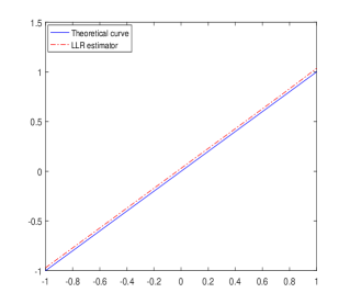
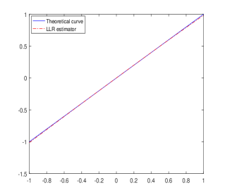
Figure 1: $\quad\mu(\cdot)$, $\widehat{\mu}(\cdot)$ with C.P.$\approx 30\%$ for $n=100,300$ and $500$ respectively.

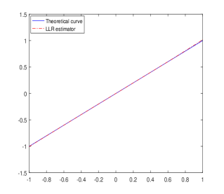
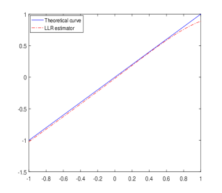
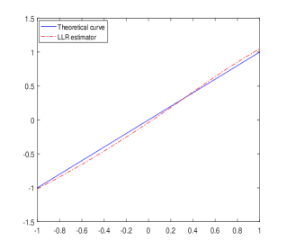
Figure 2: $\quad\mu(\cdot)$, $\widehat{\mu}(\cdot)$ with $n=300$ for C.P.$\approx 8,25$ and $60\%$ respectively.

Figure 3: $\quad\mu(\cdot)$, $\widehat{\mu}(\cdot)$ and $\mu_{n}(\cdot)$ with $n=300$ for C.P.$\approx 10,35$ and $65\%$ respectively.

Table 1: Comparative table of MSE.

C.P.	n	CR	LLR
	100	0.0158	0.0011
10	300	0.0024	0.0003
	500	2.48 $\times 10^{-4}$	2.32 $\times 10^{-6}$
	100	0.0836	0.0025
30	300	0.0473	0.0020
	500	0.0108	8.10 $\times 10^{-4}$
	100	0.0611	0.1181
50	300	0.2321	0.0228
	500	0.0258	0.0064

In Figure 1-3, it can be seen that for $(i)$ the LLR estimator performs better as increasing of the sample size $n$; $(ii)$ the estimator quality is affected by the C.P. but resists and keeps close to the theoretical curve; $(iii)$ the LLR and CR estimators are almost indistinguishable when the censorship rate is low. Notably, the CR estimator is sensitive to the effect of censorship, which is visible on the edges, unlike the LLR estimator, which resists the edge and remains stuck to the theoretical curve. In the Table 1, we take different values of C.P. and report the mean squared error (MSE) of the LLR estimator and CR estimator. We can see that the LLR estimator performs better when the sample size increases and is only slightly affected by the percentage of observed data.

5 Proofs and Auxiliary results

Proof of Proposition 1.3. We retain all the notation from Section 2 and let denote by

$$\widehat{S}_{\ell}(x)=\frac{1}{nh}\sum_{i=1}^{n}\widehat{Z}^{\star}_{i}(X_{i}-x)^{\ell}K_{i},\quad\quad\widetilde{S}_{\ell}(x)=\frac{1}{nh}\sum_{i=1}^{n}{Z}^{\star}_{i}(X_{i}-x)^{\ell}K_{i}\quad\text{for}\quad\ell=0,1,$$

and

$$\widehat{T}_{\ell}(x)=\frac{1}{nh}\sum_{i=1}^{n}(X_{i}-x)^{\ell}K_{i}\quad\text{for}\quad\ell=0,1,2.$$

Consider now the following decomposition:

$$\left|\widehat{\mu}_{1}(x)-\widetilde{\mu}_{1}(x)\right| =\left|\widehat{S}_{0}(x)\widehat{T}_{2}(x)-\widehat{S}_{1}(x)\widehat{T}_{1}(x)-\widetilde{S}_{0}(x)\widehat{T}_{2}(x)+\widetilde{S}_{1}(x)\widehat{T}_{1}(x)\right|$$

$$\leq\left|\widehat{T}_{2}(x)-\mathbb{E}[\widehat{T}_{2}(x)]\right|\times\left|\widehat{S}_{0}(x)-\widetilde{S}_{0}(x)\right|+\left|\mathbb{E}[\widehat{T}_{2}(x)]\left(\widehat{S}_{0}(x)-\widetilde{S}_{0}(x)\right)\right|$$

$$+\left|\widehat{T}_{1}(x)-\mathbb{E}[\widehat{T}_{1}(x)]\right|\times\left|\widehat{S}_{1}(x)-\widetilde{S}_{1}(x)\right|+\left|\mathbb{E}[\widehat{T}_{1}(x)]\left(\widehat{S}_{1}(x)-\widetilde{S}_{1}(x)\right)\right|,$$

We then state and prove Lemma 1-3 which are needed in Proposition 1.3.

Lemma 1

Under Assumptions A2 and A3, we have for $\ell=0,1$

$$\sup_{x\in\mathscr{C}}|\widehat{S}_{\ell}(x)-\widetilde{S}_{\ell}(x)|=\text{O}_{a.s.}\left(\sqrt{\frac{\log\log n}{n}}\right)\;\;\;\text{as}\;\;\;n\rightarrow\infty.$$

Proof of Lemma 1. For $\ell=0,1,$ we have

$$\sup_{x\in\mathscr{C}}\left|\widehat{S}_{\ell}(x)-\widetilde{S}_{\ell}(x)\right| =\sup_{x\in\mathscr{C}}\left|\frac{1}{nh}\sum_{j=1}^{n}\widehat{Z}_{j}^{\star}(X_{j}-x)^{\ell}K_{j}-\frac{1}{nh}\sum_{j=1}^{n}Z_{j}^{\star}(X_{j}-x)^{\ell}K_{j}\right|$$

$$\leq\sup_{x\in\mathscr{C}}\left|\frac{1}{nh}\sum_{j=1}^{n}Z_{j}(X_{j}-x)^{\ell}K_{j}\left(\frac{1}{\bar{G}_{n}(Z_{j})}-\frac{1}{\bar{G}(Z_{j})}\right)\right|$$

$$\leq\frac{1}{\bar{G}^{2}(\tau_{H})}\sup_{t\leq\tau_{H}}\left|\bar{G}_{n}(t)-\bar{G}(t)\right|\times\sup_{x\in\mathscr{C}}\left|\frac{1}{nh}\sum_{j=1}^{n}Z_{j}(X_{j}-x)^{\ell}K_{j}\right|$$

$$=:\sup_{t\leq\tau_{H}}\mathscr{L}_{1}(t)\times\sup_{x\in\mathscr{C}}\left|\mathscr{L}_{2}(x)\right|.$$

For $\mathscr{L}_{1}$, using Lemma 4.2. in Deheuvels and Einmahl (2000), we get

$$\sup_{t\leq\tau_{H}}\mathscr{L}_{1}(t)=\text{O}_{a.s.}\left(\sqrt{\frac{\log\log n}{n}}\right).$$ (9)

For $\mathscr{L}_{2}$, under Assumptions A2 and A3, using the strong large law numbers, change of variable and Taylor expansion around $x$, we have

$$\sup_{x\in\mathscr{C}}\left|\mathscr{L}_{2}(x)\right| \leq C\sup_{x\in\mathscr{C}}\left|\mathbb{E}\left[h^{-1}(X_{1}-x)^{\ell}K_{1}\right]\right|$$ (10)

$$= h^{\ell+1}\sup_{x\in\mathscr{C}}|f^{\prime}(x)|\int v^{\ell+1}K(v)dv.$$

Finally, combining the results in (9) and (10) concludes the proof of Lemma 1.

Lemma 2

Under Assumption A1, A2 and A3, we have for $\ell=0,1,2$

$$\sup_{x\in\mathscr{C}}\left|\widehat{T}_{\ell}(x)-\mathbb{E}[\widehat{T}_{\ell}(x)]\right|=\text{O}_{a.s.}\left(\sqrt{\frac{\log n}{nh}}\right)\;\;\;\text{as}\;\;\;n\rightarrow\infty.$$

Proof of Lemma 2. Let $b_{n}=n^{-1/2\nu}$ for $\nu>0$ and cover the compact set $\mathscr{C}$ by $\displaystyle{\cup_{i=1}^{d_{n}}}(x_{i}-b_{n},x_{i}+b_{n})$ with $d_{n}=\text{O}(n^{1/2\nu})$. Let

$$\mathscr{C}_{n}=\{x_{i}-b_{n};\,x_{i}+b_{n},\;1\leq i\leq d_{n}\},$$

the extremities of the latter subdivision, Then

$$\sup_{x\in\mathscr{C}}|\widehat{T}_{\ell}(x)-\mathbb{E}[\widehat{T}_{\ell}(x)]|\leq\max_{1\leq i\leq d_{n}}\max_{x\in\mathscr{C}_{n}}|\widehat{T}_{\ell}(x)-\mathbb{E}[\widehat{T}_{\ell}(x)]|+2^{\nu}Cb_{n}^{\nu}.$$ (11)

Since $b_{n}=n^{-1/2\nu}$ then

$$b_{n}^{\nu}=\text{O}\left(\sqrt{\frac{\log n}{nh}}\right).$$

Then for all $\varepsilon>0$, we have

$$\mathbb{P}\left(\max_{x\in\mathscr{C}_{n}}|\widehat{T}_{\ell}(x)-\mathbb{E}[\widehat{T}_{\ell}(x)]|>\varepsilon\right)\leq\sum_{x\in\mathscr{C}_{n}}\mathbb{P}\left(|\widehat{T}_{\ell}(x)-\mathbb{E}[\widehat{T}_{\ell}(x)]|>\varepsilon\right).$$

Let us write for $\ell=0,1,2$ and $x\in\mathscr{C}_{n}$

$$\widehat{T}_{\ell}(x)-\mathbb{E}[\widehat{T}_{\ell}(x)] =\frac{1}{n}\sum_{i=1}^{n}\frac{(X_{i}-x)^{\ell}K_{i}-\mathbb{E}\left[(X_{i}-x)^{\ell}K_{i}\right]}{h}$$

$$=:\frac{1}{n}\sum_{i=1}^{n}\mathscr{A}_{\ell,i}(x).$$

Since an almost complete property holds almost surely, we apply Corollary 1. For that, we focus on the absolute moments of $\mathscr{A}_{\ell,i}(x)$

$$\mathbb{E}|\mathscr{A}_{\ell,i}(x)|^{m} =h^{-m}\mathbb{E}\left|\sum_{k=0}^{m}c_{k,m}\left((X_{i}-x)^{\ell}K_{i}\right)^{k}\mathbb{E}\left[(X_{i}-x)^{\ell}K_{i}\right]^{m-k}\right|$$

$$\leq h^{-m}\sum_{k=0}^{m}c_{k,m}\left|\mathbb{E}\left[\left((X_{1}-x)^{\ell}K_{1}\right)^{k}\right]\mathbb{E}\left[(X_{1}-x)^{\ell}K_{1}\right]^{m-k}\right|.$$

On the one hand, using conditional expectation property, A2 and A3, we have

$$\mathbb{E}\left[\left((X_{1}-x)^{\ell}K_{1}\right)^{k}\right] =h^{\ell k+1}\int v^{\ell k}K^{k}(v)f(x+vh)dv$$

and

$$\mathbb{E}\left[(X_{1}-x)^{\ell}K_{1}\right]^{m-k} =\left(h^{\ell+1}\int v^{\ell}K(v)f(x+vh)dv\right)^{m-k}$$

then, for $\ell=0,1,2$ and $\forall m\geq 2$

$$\mathbb{E}|\mathscr{A}_{\ell,1}(x)|^{m} =\text{O}(h^{m\ell-k+1}) =\text{O}(\max_{1\leq k\leq m}h^{-k+1}) =\text{O}(h^{-m+1}).$$

We can now apply Corollary 2. Choosing $a^{2}=h^{-1}$ we get

$$\mathbb{P}\left(\left|\widehat{T}_{\ell}(x)-\mathbb{E}[\widehat{T}_{\ell}(x)]\right|>\varepsilon\right) =\mathbb{P}\left(\left|\sum_{i=1}^{n}\mathscr{A}_{\ell,i}(x)\right|>\varepsilon n\right)$$

$$\leq 2\exp\left(-\frac{\varepsilon^{2}nh}{2(1+\varepsilon)}\right).$$

Hence, for $\varepsilon=\varepsilon_{0}\left(\frac{\log n}{nh}\right)^{1/2}$ and $n$ large enough, we get

$$\mathbb{P}\left(\left|\widehat{T}_{\ell}(x)-\mathbb{E}[\widehat{T}_{\ell}(x)]\right|>\varepsilon\right)\leq 2\exp\left(-\frac{\varepsilon_{0}^{2}}{4}\log n\right)=2n^{-\frac{\varepsilon_{0}^{2}}{4}}.$$

It follows that

$$\sum_{x\in\mathscr{C}_{n}}\mathbb{P}\left(|\widehat{T}_{\ell}(x)-\mathbb{E}[\widehat{T}_{\ell}(x)]|>\varepsilon\right)\leq 4n^{-\frac{\varepsilon_{0}^{2}}{4}+\frac{1}{2\nu}}.$$

Finally, an appropriate choice of $\varepsilon_{0}$ yields an upper bound of order $n^{-3/2}$ which by Borel-Cantelli’s lemma completes the proof of Lemma 2.

Lemma 3

Under Assumptions A1, A2 and A3, we have for $\ell=0,1,2$

$$\mathbb{E}[\widehat{T}_{\ell}(x)]=\text{O}(h^{\ell}).\;\;\;$$

Proof of Lemma 3. For $\ell=0,1,2$, using a change of variable and Taylor expansion for $\xi\in[x,x+hv]$, we have

$$\mathbb{E}[\widehat{T}_{\ell}(x)] =h^{\ell}\int v^{\ell}K(v)f(x+hv)dt$$

$$=h^{\ell}f(x)\int v^{\ell}K(v)dv+h^{\ell+1}\int v^{\ell+1}K(v)f^{\prime}(\xi)dv$$

under Assumptions A1, A2 and A3 we get the result. Then, combining the results in Lemma 1 with Lemma 2 and Lemma 1 with Lemma 3 we get the result of Proposition 1. Proof of Proposition 1.4. By similar reasoning than the Proof of Proposition 1.3, we remark that:

$$\mathscr{B}_{4}(x) =\left\{\widetilde{S}_{0}(x)\widehat{T}_{2}(x)-\mathbb{E}\left[\widetilde{S}_{0}(x)\widehat{T}_{2}(x)\right]\right\}-\left\{\widetilde{S}_{1}(x)\widehat{T}_{1}(x)-\mathbb{E}\left[\widetilde{S}_{1}(x)\widehat{T}_{1}(x)\right]\right\}$$

$$=:\mathscr{B}_{4,1}(x)-\mathscr{B}_{4,2}(x).$$

On the one hand

$$\mathscr{B}_{4,1}(x) = \left(\widetilde{S}_{0}(x)-\mathbb{E}\left[\widetilde{S}_{0}(x)\right]\right)\left(\widehat{T}_{2}(x)-\mathbb{E}\left[\widehat{T}_{2}(x)\right]\right)+\left(\widehat{T}_{2}(x)-\mathbb{E}\left[\widehat{T}_{2}(x)\right]\right)\mathbb{E}\left[\widetilde{S}_{0}(x)\right]$$ (12)

$$+ \left(\widetilde{S}_{0}(x)-\mathbb{E}\left[\widetilde{S}_{0}(x)\right]\right)\mathbb{E}\left[\widehat{T}_{2}(x)\right]+\mathbb{E}\left[\widetilde{S}_{0}(x)\right]\mathbb{E}\left[\widehat{T}_{2}(x)\right]-\mathbb{E}\left[\widetilde{S}_{0}(x)\widehat{T}_{2}(x)\right].$$

On the other hand

$$\mathscr{B}_{4,2}(x) = \left(\widetilde{S}_{1}(x)-\mathbb{E}\left[\widetilde{S}_{1}(x)\right]\right)\left(\widehat{T}_{1}(x)-\mathbb{E}\left[\widehat{T}_{1}(x)\right]\right)+\left(\widehat{T}_{1}(x)-\mathbb{E}\left[\widehat{T}_{1}(x)\right]\right)\mathbb{E}\left[\widetilde{S}_{1}(x)\right]$$ (13)

$$+ \left(\widetilde{S}_{1}(x)-\mathbb{E}\left[\widetilde{S}_{1}(x)\right]\right)\mathbb{E}\left[\widehat{T}_{1}(x)\right]+\mathbb{E}\left[\widetilde{S}_{1}(x)\right]\mathbb{E}\left[\widehat{T}_{1}(x)\right]-\mathbb{E}\left[\widetilde{S}_{1}(x)\widehat{T}_{1}(x)\right].$$

It remains to study each term in the decompositions (12) and (13). For that, let us consider the following Lemmas.

Lemma 4

Under Assumption A1, A2, A4 and A5, we have for $\ell=0,1,$

$$\sup_{x\in\mathscr{C}}\left|\widetilde{S}_{\ell}(x)-\mathbb{E}\left[\widetilde{S}_{\ell}(x)\right]\right|=\text{O}_{a.s.}\left(\sqrt{\frac{\log n}{n\,h}}\right)\quad\quad\quad\text{as}\quad n\rightarrow\infty.$$

Proof of Lemma 4. The proof is very similar to that of Lemma 2. The same notations of Lemma 2 are used.

$$\sup_{x\in\mathscr{C}}|\widetilde{S}_{\ell}(x)-\mathbb{E}[\widetilde{S}_{\ell}(x)]|\leq\max_{1\leq j\leq d_{n}}\max_{x\in\mathscr{C}_{n}}|\widetilde{S}_{\ell}(x)-\mathbb{E}[\widetilde{S}_{\ell}(x)]|+2^{\nu}Cb_{n}^{\nu}.$$

Observe that

$$\mathbb{P}\left(\max_{x\in\mathscr{C}_{n}}|\widetilde{S}_{\ell}(x)-\mathbb{E}[\widetilde{S}_{\ell}(x)]|>\varepsilon\right)\leq\sum_{x\in\mathscr{C}_{n}}\mathbb{P}\left(|\widetilde{S}_{\ell}(x)-\mathbb{E}[\widetilde{S}_{\ell}(x)]|>\varepsilon\right).$$

Let us write for $\ell=0,1$ and $x\in\mathscr{C}_{n}$

$$\widetilde{S}_{\ell}(x)-\mathbb{E}[\widetilde{S}_{\ell}(x)] =\frac{1}{n}\sum_{j=1}^{n}\frac{Z^{\star}_{j}(X_{j}-x)^{\ell}K_{j}-\mathbb{E}\left[Z^{\star}_{j}(X_{j}-x)^{\ell}K_{j}\right]}{h}$$

$$=:\frac{1}{n}\sum_{j=1}^{n}\mathscr{R}_{\ell,j}(x).$$

In order to apply Corollary 2, we focus on the absolute moments of $\mathscr{R}_{\ell,j}(x)$ for $\ell=0,1$

$$\mathbb{E}|\mathscr{R}_{\ell,j}(x)|^{m} \leq h^{-m}\sum_{k=0}^{m}c_{k,m}\left|\mathbb{E}\left[\left(Z^{\star}_{1}(X_{1}-x)^{\ell}K_{1}\right)^{k}\right]\mathbb{E}\left[Z^{\star}_{1}(X_{1}-x)^{\ell}K_{1}\right]^{m-k}\right|.$$

On the one hand, using conditional expectation property, under A5 for $m\geq k$, we get

$$\mathbb{E}\left[\left(Z^{\star}_{1}(X_{1}-x)^{\ell}K_{1}\right)^{k}\right] = \mathbb{E}\left[(X_{1}-x)^{\ell k}K_{1}^{k}\mathbb{E}[Z^{\star,k}_{1}|X_{1}]\right]$$ (14)

$$= \int(u-x)^{\ell k}K^{k}\left(\frac{u-x}{h}\right)\mathbb{E}[Z^{\star,k}_{1}|X_{1}=u]f_{X}(u)du$$

with

$$\mathbb{E}[Z^{\star,k}_{1}|X_{1}=u] = \mathbb{E}\left[\frac{Z_{1}^{k}}{\bar{G}^{k-1}(Y_{1})}\big{|}X_{1}=u\right]$$ (15)

$$\leq \frac{1}{\bar{G}^{k-1}(\tau_{H})}\int z^{k}f_{Z|X}(z|u)dz.$$

We replace (15) in (14), under A5, we get

$$\mathbb{E}\left[\left(Z^{\star}_{1}(X_{1}-x)^{\ell}K_{1}\right)^{k}\right] =\mathbb{E}\left[(X_{1}-x)^{\ell k}K_{1}^{k}\mathbb{E}[Z^{\star,k}_{1}|X_{1}]\right]$$

$$=\int(u-x)^{\ell k}K^{k}\left(\frac{u-x}{h}\right)\mathbb{E}[Z^{\star,k}_{1}|X_{1}=u]f_{X}(u)du$$

$$\leq\frac{1}{\bar{G}^{k-1}(\tau_{H})}\int(u-x)^{\ell k}K^{k}\left(\frac{u-x}{h}\right)\int z^{k}f_{Z|X}(z|u)f_{X}(u)dzdu$$

$$=\frac{1}{\bar{G}^{k-1}(\tau_{H})}\int(u-x)^{\ell k}K^{k}\left(\frac{u-x}{h}\right)\upsilon_{k}(u)du$$

$$=\frac{h^{\ell k+1}}{\bar{G}^{k-1}(\tau_{H})}\int s^{\ell k}K^{k}(s)\upsilon_{k}(x+hs)ds.$$

On the other hand, under (2) and analogously to the previous development, we get

$$\mathbb{E}\left[Z^{\star}_{1}(X_{1}-x)^{\ell}K_{1}\right]^{m-k} =\mathbb{E}\left[(X_{1}-x)^{\ell}K_{1}\mathbb{E}[Z^{\star}_{1}|X_{1}]\right]^{m-k}$$

$$=\mathbb{E}\left[(X_{1}-x)^{\ell}K_{1}\mathbb{E}\left[Z_{1}|X_{1}\right]\right]^{m-k}$$

$$=\left(\int(u-x)^{\ell}K\left(\frac{u-x}{h}\right)\mu(u)f(u)du\right)^{m-k}$$

$$=\left(h^{\ell+1}\int v^{\ell}K(v)S_{0}(x+vh)dv\right)^{m-k}.$$

By A2 and A4, for $\ell=0,1$ and $\forall\;m\geq 2$

$$\mathbb{E}|\mathscr{R}_{\ell,1}(x)|^{m} \leq\text{O}(h^{m\ell-k+1}) =\text{O}(\max_{1\leq k\leq m}h^{-k+1}) =\text{O}(h^{-m+1}).$$

Now, we can apply Corollary 2. By choosing $a^{2}=h^{-1}$, $\varepsilon=\varepsilon_{0}\left(\frac{\log n}{nh}\right)^{1/2}$ and for $n$ large enough, we get

$$\mathbb{P}\left(\left|\widetilde{S}_{\ell}(x)-\mathbb{E}[\widetilde{S}_{\ell}(x)]\right|>\varepsilon\right) =\mathbb{P}\left(\left|\sum_{j=1}^{n}\mathscr{R}_{\ell,j}(x)\right|>n\varepsilon\right)$$

$$\leq 2\exp\left(-\frac{\varepsilon_{0}^{2}}{4}\log n\right)=2n^{-\frac{\varepsilon_{0}^{2}}{4}}.$$

It follows that

$$\sum_{x\in\mathscr{C}_{n}}\mathbb{P}\left(|\widetilde{S}_{\ell}(x)-\mathbb{E}[\widetilde{S}_{\ell}(x)]|>\varepsilon\right)\leq 4n^{-\frac{\varepsilon_{0}^{2}}{4}+\frac{1}{2\nu}}.$$

Finally, an appropriate choice of $\varepsilon_{0}$ yields to an upper bound of order $n^{-3/2}$ which by Borel-Cantelli’s lemma completes the proof of Lemma 4.

Lemma 5

Under Assumptions A1, A2 and A4, we have for $\ell=0,1,$

$$\mathbb{E}[\widetilde{S}_{\ell}(x)]=\text{O}(h^{\ell})\quad\quad\quad\text{as}\quad n\rightarrow\infty.$$

Proof of Lemma 5. For $\ell=0,1$, using a change of variable, Taylor expansion for $\xi\in]x,x+vh[$ and under A1, A2 and A4, we have

$$\mathbb{E}\left[\widetilde{S}_{\ell}(x)\right] =\int(hv)^{\ell}K(v)S_{0}(x+hv)dv$$

$$=h^{\ell}S_{0}(x)\int v^{\ell}K(v)dv+h^{\ell+1}\int v^{\ell+1}K(v)S_{0}^{\prime}(\xi)dv.$$

Now, it remains to study the quantity $\mathbb{E}\left[\widetilde{S}_{0}(x)\right]\mathbb{E}\left[\widehat{T}_{2}(x)\right]-\mathbb{E}\left[\widetilde{S}_{0}(x)\widehat{T}_{2}(x)\right]$. To do that, let consider the following Lemma.

Lemma 6

Under Assumptions A1-A4, we have

$$\text{Cov}(\widetilde{S}_{0}(x),\widehat{T}_{2}(x))=\text{o}\left(\sqrt{\frac{\log n}{nh}}\right)\quad\quad\quad\text{as}\quad n\rightarrow\infty.$$

Proof of Lemma 6. By a change of variable, Taylor expansion and under A1-A4, we have

$$\text{Cov}(\widetilde{S}_{0}(x),\widehat{T}_{2}(x)) =\frac{1}{(nh)^{2}}\sum_{j=1}^{n}\sum_{i=1}^{n}\left[\mathbb{E}\left(Z_{j}^{\star}(X_{i}-x)^{2}K_{i}K_{j}\right)-\mathbb{E}\left(Z_{j}^{\star}K_{j}\right)\mathbb{E}\left((X_{i}-x)^{2}K_{i}\right)\right]$$

$$=\left(\frac{n(n-1)-n^{2}}{(nh)^{2}}\right)\mathbb{E}\left((X_{1}-x)^{2}K_{1}\right)\mathbb{E}\left(Z_{1}^{\star}K_{1}\right)+\frac{n}{(nh)^{2}}\mathbb{E}\left(Z_{1}^{\star}(X_{1}-x)^{2}K_{1}^{2}\right)$$

$$=O\left(\frac{h}{n}\right)$$

which is negligible with respect to $\sqrt{\frac{\log n}{nh}}$.

Lemma 7

Under Assumptions A1-A4, we have

$$\text{Cov}(\widetilde{S}_{1}(x),\widehat{T}_{1}(x))=\text{o}\left(\sqrt{\frac{\log n}{nh}}\right)\quad\quad\quad\text{as}\quad n\rightarrow\infty.$$

Proof of Lemma 7. By a change of variable, Taylor expansion and underA1-A4, we have

$$\text{Cov}(\widetilde{S}_{1}(x),\widehat{T}_{1}(x)) =\frac{1}{(nh)^{2}}\sum_{j=1}^{n}\sum_{i=1}^{n}\left[\mathbb{E}\left(Z_{j}^{\star}(X_{i}-x)(X_{j}-x)K_{i}K_{j}\right)-\mathbb{E}(Z_{j}^{\star}K_{j})\mathbb{E}\left((X_{i}-x)K_{i}\right)\right]$$

$$=\left(\frac{n(n-1)-n^{2}}{(nh)^{2}}\right)\mathbb{E}\left((X_{1}-x)K_{1}\right)\mathbb{E}\left(Z_{1}^{\star}(X_{1}-x)K_{1}\right)+\frac{n}{(nh)^{2}}\mathbb{E}\left(Z_{1}^{\star}(X_{1}-x)^{2}K_{1}^{2}\right)$$

$$=O\left(\frac{h^{2}}{n}\right)$$

which is negligible with respect to $\sqrt{\frac{\log n}{nh}}$. Then combining the results in Lemma 2 and Lemma 4 with Lemma 2 and Lemma 5 with Lemma 3 and Lemma 4 in addition to Lemma 6 and Lemma 7 concludes the proof of the Proposition 1.4.
Proof of Proposition 1.2. This proof is similar to that of Proposition 1.4. We use the same notation used in Lemma 2 and the following decomposition

$$\mathscr{B}_{2}(x) =\widehat{T}_{0}(x)\widehat{T}_{2}(x)-\widehat{T}_{1}^{2}(x)-\mathbb{E}[\widehat{T}_{0}(x)\widehat{T}_{2}(x)-\widehat{T}_{1}^{2}(x)]$$

$$=\left\{\widehat{T}_{0}(x)\widehat{T}_{2}(x)-\mathbb{E}[\widehat{T}_{0}(x)\widehat{T}_{2}(x)]\right\}-\left\{\widehat{T}_{1}^{2}(x)-\mathbb{E}[\widehat{T}_{1}^{2}(x)]\right\}$$

$$=:\mathscr{B}_{2,1}(x)-\mathscr{B}_{2,2}(x).$$

On the one hand

$$\mathscr{B}_{2,1}(x) = (\widehat{T}_{0}(x)-\mathbb{E}[\widehat{T}_{0}(x)])(\widehat{T}_{2}(x)-\mathbb{E}[\widehat{T}_{2}(x)])+\mathbb{E}[\widehat{T}_{0}(x)](\widehat{T}_{2}(x)-\mathbb{E}[\widehat{T}_{2}(x)])$$ (16)

$$+ \mathbb{E}[\widehat{T}_{2}(x)](\widehat{T}_{0}(x)-\mathbb{E}[\widehat{T}_{0}(x)])+\mathbb{E}[\widehat{T}_{2}(x)]\mathbb{E}[\widehat{T}_{0}(x)]-\mathbb{E}[\widehat{T}_{0}(x)\widehat{T}_{2}(x)].$$

On the other hand

$$\mathscr{B}_{2,2}(x)=\widehat{T}_{1}^{2}(x)-\mathbb{E}[\widehat{T}_{1}^{2}(x)]=\text{Var}[\widehat{T}_{1}(x)].$$ (17)

it remains to study each term in (16) and (17). The terms $\mathbb{E}[\widehat{T}_{\ell}(x)]$ and $\widehat{T}_{\ell}(x)-\mathbb{E}[\widehat{T}_{\ell}(x)]$ for $\ell=0,1,2$ were considered in Lemma 3 and Lemma 2 respectively. For the others terms, we consider the following Lemmas.

Lemma 8

Under Assumptions A1, A2 and A3, for $\ell=0,1,2$, we have

$$\text{Var}[\widehat{T}_{\ell}(x)]=\text{o}\left(\sqrt{\frac{\log n}{nh}}\right)\quad\quad\quad\text{as}\quad n\rightarrow\infty.$$

Proof of Lemma 8. For $\ell=0,1,2,$ with a change of variable and Taylor expansion with $\xi\in]x,x+hs[$, we have

$$\mathbb{E}[\widehat{T}_{\ell}^{2}(x)] =\frac{1}{nh^{2}}\int(u-x)^{2\ell}K^{2}\left(\frac{u-x}{h}\right)f(u)du$$

$$=\frac{1}{nh}\int(sh)^{2\ell}K^{2}(s)f(x+hs)ds$$

$$=\frac{1}{nh}\left\{h^{2\ell}f(x)\int s^{2\ell}K^{2}(s)ds+h^{2\ell+1}\int s^{2\ell+1}K^{2}(s)f^{\prime}(\xi)ds\right\}.$$

Under A1, A2 and A3 we get the result. Furthermore the result is $\text{o}\left(\sqrt{\frac{\log n}{nh}}\right)$.

Lemma 9

Under Assumptions A1-A3, we have

$$\text{Cov}(\widehat{T}_{0}(x),\widehat{T}_{2}(x))=\text{o}\left(\sqrt{\frac{\log n}{nh}}\right)\quad\quad\quad\text{as}\quad n\rightarrow\infty.$$

Proof of Lemma 9. By a change of variable and Taylor expansion we have

$$\text{Cov}(\widehat{T}_{0}(x),\widehat{T}_{2}(x)) =\frac{1}{(nh)^{2}}\sum_{j=1}^{n}\sum_{i=1}^{n}\left[\mathbb{E}\left((X_{i}-x)^{2}K_{i}K_{j}\right)-\mathbb{E}\left(K_{j}\right)\mathbb{E}\left((X_{i}-x)^{2}K_{i}\right)\right]$$

$$=\frac{1}{n^{2}h^{2}}\left\{(n(n-1)-n^{2})\mathbb{E}\left[K_{1}\right]\mathbb{E}\left[(X_{1}-x)^{2}K_{1}\right]+\mathbb{E}\left[(X_{1}-x)^{2}K^{2}_{1}\right]\right\}$$

$$=O\left(\frac{h^{2}}{n}\right).$$

Under Assumptions A1-A3, we get the result. Then, combining the results in Lemma 2 and Lemma 2 with Lemma 3 in addition to the results in Lemma 8 and Lemma 9 conclude the proof of the Proposition 1.2.
Proof of corollary 1. There exists $\Gamma>0$, such that for all $x\in\mathscr{C},\;\mathbb{E}[\widehat{\mu}_{0}(x)]\geq\Gamma$. Therefore $\displaystyle\inf_{x\in\mathscr{C}}\widehat{\mu}_{0}(x)\leq\frac{\Gamma}{2}$ implies that there exists $x\in\mathscr{C}$ such that $|\mathbb{E}[\widehat{\mu}_{0}(x)]-\widehat{\mu}_{0}(x)|\geq\frac{\Gamma}{2}$ which gives

$$\sup_{x\in\mathscr{C}}\Big{|}\mathbb{E}[\widehat{\mu}_{0}(x)]-\widehat{\mu}_{0}(x)\Big{|}\geq\frac{\Gamma}{2}.$$

Thus, the result of Proposition 1.2. allows to write that for $\frac{\Gamma}{2}=\Gamma^{\prime}$:

$$\sum_{n}\mathbb{P}\left(\inf_{x\in\mathscr{C}}\widehat{\mu}_{0}(x)\leq\Gamma^{\prime}\right)\leq\sum_{n}\mathbb{P}\left(\sup_{x\in\mathscr{C}}\Big{|}\mathbb{E}[\widehat{\mu}_{0}(x)]-\widehat{\mu}_{0}(x)\Big{|}\leq\Gamma^{\prime}\right)<\infty.$$

Proof of Proposition 1.1. Let consider

$$|\mathscr{B}_{1}(x)|=\left|\frac{\mathbb{E}\left[\widetilde{\mu}_{1}(x)\right]}{\mathbb{E}\left[\widehat{\mu}_{0}(x)\right]}-\mu(x)\right| =\left|\frac{\mathbb{E}\left[\widetilde{\mu}_{1}(x)\right]-\mu(x)\mathbb{E}\left[\widehat{\mu}_{0}(x)\right]}{\mathbb{E}\left[\widehat{\mu}_{0}(x)\right]}\right|$$

$$=\left|\frac{h^{-2}\left\{\mathbb{E}[w_{1,2}(x)Z^{\star}_{2}]-\mu(x)\mathbb{E}\left[w_{1,2}(x)\right]\right\}}{h^{-2}\mathbb{E}\left[w_{1,2}(x)\right]}\right|$$

$$=\left|\frac{\mathbb{E}\left[w_{1,2}(x)\left\{\mathbb{E}[Z^{\star}_{2}|X_{2}]-\mu(x)\right\}\right]}{\mathbb{E}[w_{1,2}(x)]}\right|$$

$$=\left|\frac{\mathbb{E}\left[w_{1,2}(x)\left(\mu(X_{2})-\mu(x)\right)\right]}{\mathbb{E}\left[w_{1,2}(x)\right]}\right|$$

$$=\left|\mu(X_{2})-\mu(x)\right|.$$

Thus, under A6, we have

$$\sup_{x\in\mathscr{C}}|\mathscr{B}_{1}(x)|\leq C|X_{2}-x|^{\nu}\leq Ch^{\nu}.$$

Finally, by summing the results in Proposition 1.1-Proposition 1.4, we get the proof of Theorem 1.

Corollary 2

(A.8. p. 234 in Ferraty and Vieu (2006)) . Let $U_{i}$ be a sequence of independent r.v. with zero mean. If $\forall\;m\geq 2$, $\exists\;C_{m}>0$, $\mathbb{E}[|U_{1}^{m}|]\leq C_{m}a^{2(m-1)}$, we have

$$\forall\varepsilon>0,\;\;\;\mathbb{P}\left(\left|\sum_{i=1}^{n}U_{i}\right|>n\varepsilon\right)\leq 2\exp\left\{-\frac{\varepsilon^{2}n}{2a^{2}(1+\varepsilon)}\right\}.$$

Concluding remarks

In this note, we study a local linear regression function estimator and show that this method has advantages with respect to the classical kernel estimator. On simulated data we show that the LL method is more efficient than the classical kernel method. On the one hand, it mitigates edge effects and on the other hand, it remains efficient when the censoring rate increases substantially. We point out that the method proposed in Cai (2003) with two weights where the first is standard kernel for smoothing and the second which is the Kaplan and Meier (1958) estimator. The resulting estimator is interesting, however the author does not use a weighting in the denominator with the survival law of the censoring random variable. Recall that El Ghouch and Van Keilegom (2008) estimated the regression function by applying polynomial local linear regression techniques using Beran’s estimator. Their conditions need to have a result about conditional law on the censored random variable that in our case we do not use it. Furthermore their uniform result is given only in probability. We point out and to the best of our knowledge, the type of our result has never been obtained.