Realizable Hyperuniform and Nonhyperuniform Particle Configurations with Targeted Spectral Functions via Effective Pair Interactions

Abstract

The capacity to identify realizable many-body configurations associated with targeted functional forms for the pair correlation function $g_{2}(r)$ or its corresponding structure factor $S(k)$ is of great fundamental and practical importance. While there are obvious necessary conditions that a prescribed structure factor at number density $\rho$ must satisfy to be configurationally realizable, sufficient conditions are generally not known due to the infinite degeneracy of configurations with different higher-order correlation functions. A major aim of this paper is to expand our theoretical knowledge of the class of pair correlation functions or structure factors that are realizable by classical disordered ensembles of particle configurations, including exotic “hyperuniform” varieties. We first introduce a theoretical formalism that provides a means to draw classical particle configurations from canonical ensembles with certain pairwise-additive potentials that could correspond to targeted analytical functional forms for the structure factor. This formulation enables us to devise an improved algorithm to construct systematically canonical-ensemble particle configurations with such targeted pair statistics, whenever realizable. As a proof-of-concept, we test the algorithm by targeting several different structure factors across dimensions that are known to be realizable and one hyperuniform target that is known to be nontrivially unrealizable. Our algorithm succeeds for all realizable targets and appropriately fails for the unrealizable target, demonstrating the accuracy and power of the method to numerically investigate the realizability problem. Subsequently, we also target several families of structure-factor functions that meet the known necessary realizability conditions but were heretofore not known to be realizable by disordered hyperuniform point configurations, including $d$-dimensional Gaussian structure factors, $d$-dimensional generalizations of the 2D one-component plasma (OCP), the $d$-dimensional Fourier duals of the previous OCP cases. Moreover, we also explore unusual nonhyperuniform targets, including “hyposurficial” and “anti-hyperuniform” examples. In all of these instances, the targeted structure factors were achieved with high accuracy, suggesting that they are indeed realizable by equilibrium configurations with pairwise interactions at positive temperatures. Remarkably, we also show that the structure factor of nonequilibrium “perfect glass” specified by two-, three-, and four-body interactions, can also be realized by equilibrium pair interactions at positive temperatures. Our findings lead us to the conjecture that any realizable structure factor corresponding to either a translationally invariant equilibrium or nonequilibrium system can be attained by an equilibrium ensemble involving only effective pair interactions. Our investigation not only broadens our knowledge of analytical functional forms for $g_{2}({\bf r})$ and $S({\bf k})$ associated with disordered point configurations across dimensions but also deepens our understanding of many-body physics. Moreover, our work can be applied to the design of materials with desirable physical properties that can be tuned by their pair statistics.

I Introduction

An outstanding problem in condensed matter physics, statistical physics and materials science is the capacity to construct, at will, many-particle configurations with prescribed correlation functions. Solutions to this general problem are of great importance both fundamentally and practically. Advances in this direction will shed light on the unsolved theoretical “realizability” problem, as described below. Practical implications of progress on this problem include the design of material microstructures with novel physical properties.

A classical many-particle system in $d$-dimensional Euclidean space $\mathbb{R}^{d}$ is completely specified by the $n$-particle probability density function $\rho_{n}({\bf r}_{1},\ldots,{\bf r}_{n})$ for all $n\geq 1$, where ${\bf r}_{1},\ldots,{\bf r}_{n}$ are the particle position vectors. In the field of statistical mechanics, the one-particle function $\rho_{1}({\bf r}_{1})$ and the two-particle function $\rho_{2}({\bf r}_{1},{\bf r}_{2})$ are the most important ones. These functions play crucial roles in determining equilibrium and nonequilibrium properties of systems and can be ascertained experimentally from scattering data Hansen and McDonald (2013). In the case of statistically homogeneous systems, which is the focus of this work, $\rho_{1}({\bf r}_{1})=\rho$, where $\rho$ is the number density, and the two-particle function depends only on the pair displacement vector ${\bf r}={\bf r}_{2}-{\bf r}_{1}$ so that $\rho_{2}({\bf r}_{1},{\bf r}_{2})=\rho^{2}g_{2}({\bf r})$, where $g_{2}({\bf r})$ is the pair correlation function. Of course, these two functions alone cannot completely specify the ensemble of configurations, i.e., there is generally a high degeneracy of configurations with the same $\rho$ and $g_{2}({\bf r})$ but different higher-order statistics ($g_{3},g_{4},\ldots$) Torquato and Stillinger (2006a); Jiao et al. (2010).

This degeneracy issue naturally leads to the following version of the realizability problem: Given a prescribed $g_{2}({\bf r})$ with a fixed positive number density $\rho$, are there ensemble configurations of particles that realize such prescribed statistics? This realizability problem has a rich and long history Yamada (1961); Lenard (1973, 1975a, 1975b); Rintoul (1997); Crawford et al. (2003); Costin and Lebowitz (2004); Koralov (2005); Stillinger and Torquato (2005); Uche et al. (2006a); Torquato and Stillinger (2006a); Kuna et al. (2007, 2011), but it is still a wide open area for research. There are obvious necessary conditions for a given pair correlation function to be realizable; for example, $g_{2}(\mathbf{r})$ must be nonnegative function i.e.,

$$g_{2}({\bf r})\geq 0\qquad\mbox{for all}\,{\bf r}.$$ (1)

Moreover, the corresponding ensemble-averaged structure factor

$$S(\mathbf{k})=1+\rho{\tilde{h}}({\bf k})\geq 0,$$ (2)

must be nonnegative for all wave vectors $\bf k$, where ${\tilde{h}}({\bf k})$ is the Fourier transform of the total correlation function $h(\mathbf{r})\equiv g_{2}({\bf r})-1$. Another simple realizability condition is that the number variance $\sigma^{2}(R)$ associated with a randomly placed spherical window of radius $R$, which is entirely determined by $\rho$ and $g_{2}(\mathbf{r})$ [or $S(\mathbf{k})$] Torquato and Stillinger (2003), must satisfy the following lower bound Yamada (1961):

$$\sigma^{2}(R)\geq\theta(1-\theta),$$ (3)

where $\theta$ be the fractional part of $\rho v_{1}(R)$ and

$$v_{1}(R)=\frac{\pi^{d/2}R^{d}}{\Gamma(1+d/2)}$$ (4)

is the volume of a $d$-dimensional sphere of radius $R$. The Yamada condition (3) is relevant only in very low dimensions, often only for $d=1$ Torquato and Stillinger (2006a). Indeed, generally speaking, it is known that the lower the space dimension, the more difficult it is to satisfy realizability conditions Torquato and Stillinger (2006a), a point elaborated in Sec. V.

Conditions for realizability have also been found for special types of many-particle systems Costin and Lebowitz (2004). Moreover, necessary and sufficient conditions for the particular class of point configurations with “hard” cores have been identified Kuna et al. (2011); rey2015regularity , but these conditions are difficult to check in practice. Thus, knowledge of necessary conditions beyond inequalities (1), (2), and (3) that can be applied to determine the realizability of general pair correlation functions are, for the most part, lacking.

This places great importance on the need to formulate algorithms to construct particle configurations that realize targeted hypothetical functional forms of the pair statistics with a certain density. Successful numerical techniques could provide theoretical guidance on attainable pair correlations. Algorithms have been devised in “direct space” to generate particle realizations that correspond to hypothetical pair correlation functions Rintoul (1997); Crawford et al. (2003), but only up to intermediate values of the pair distance $|\bf r|$. This prevents one from accurately constructing the large-scale structural characteristics of the systems.

Therefore, such direct-space methods are not suitable to explore the realizability of hypothetical functional forms of pair correlation functions that could correspond to disordered hyperuniform point configurations with high fidelity. Disordered hyperuniform many-particle systems are exotic amorphous states of matter that are like crystals in the manner in which their large-scale density fluctuations are anomalously suppressed and yet behave like typical liquids or glasses in that they are statistically isotropic without any Bragg peaks. More precisely, hyperuniform point configurations possess a structure factor $S({\bf k})$ that goes to zero as the wavenumber $|\bf k|$ vanishes Torquato and Stillinger (2003); Torquato (2018), i.e.,

$$\lim_{|{\bf k}|\to 0}S({\bf k})=0.$$ (5)

For a large class of ordered and disordered systems, the number variance $\sigma^{2}(R)$ has the following large-$R$ asymptotic behavior Torquato and Stillinger (2003); Torquato (2018):

$$\sigma^{2}(R)=2^{d}\phi\left[A\left(\frac{R}{D}\right)^{d}+B\left(\frac{R}{D}\right)^{d-1}+\ell\left(\frac{R}{D}\right)^{d-1}\right]$$ (6)

where $\phi=\rho v_{1}(D/2)$ is a dimensionless density, $D$ is a characteristic length, $A$ and $B$ are “volume” and “surface-area” coefficients, respectively, while $\ell\left(R/D\right)^{d-1}$ represents terms of lower order than $\left(R/D\right)^{d-1}$. The coefficients $A$ and $B$ can be expressed as:

$$A=\lim_{|\mathbf{k}|\rightarrow 0}S(\mathbf{k})=1+d2^{d}\phi\left<x^{d-1}\right>$$ (7)

and

$$B=-\frac{d^{2}2^{d-1}\Gamma\left(\frac{d}{2}\right)}{\Gamma\left(\frac{d+1}{2}\right)\Gamma\left(\frac{1}{2}\right)}\phi\left<x^{d}\right>$$ (8)

where $\Gamma(x)$ is the gamma function, $x=r/D$, and $<x^{d}>=\int_{0}^{\infty}x^{d}h(x)dx$ is the $d$-th moment of $h(x)$ In a perfectly hyperuniform system Torquato and Stillinger (2003), the non-negative volume coefficient vanishes, i.e., $A=0$. On the other hand, when $A>0$ and $B=0$, the system is hyposurficial; examples include homogeneous Poisson point patterns and hypothetical hard-sphere systems Torquato and Stillinger (2003). Finally, in anti-hyperuniform systems

$$\lim_{|{\bf k}|\to 0}S({\bf k})=+\infty$$ (9)

and $A$ becomes unbounded Torquato (2018). Anti-hyperuniform systems include fractals as well as systems at thermal critical points.

When the structure factor goes to zero in the limit $|{\bf k}|\rightarrow 0$ with the power-law form

$$S({\bf k})\sim|{\bf k}|^{\alpha},$$ (10)

where $\alpha>0$, hyperuniform systems can be categorized into three different classes according to the large-$R$ asymptotic scaling of the number variance Torquato (2018):

$$\sigma^{2}(R)\sim\left\{\begin{array}[]{lr}R^{d-1},\quad\alpha>1\quad\mbox{(CLASS I)}\\ R^{d-1}\ln R,\quad\alpha=1\quad\mbox{(CLASS II)}\\ R^{d-\alpha},\quad 0<\alpha<1\quad\mbox{(CLASS III)}\end{array}\right.$$ (14)

Class I is the strongest form of hyperuniformity in the sense that it is the scaling that provides the greatest suppression of large-scale density fluctuations.

Disordered hyperuniform systems have attracted great attention because of their deep connections to problems that arise in physics, materials science, mathematics and biology Chremos and Douglas (2017); Torquato (2018); Ghosh and Lebowitz (2018); Brauchart et al. (2018); Crowley et al. (2018); Lei et al. (2019); Lacroix-A-Chez-Toine et al. (2019) as well as for their emerging technological importance, including disordered cellular solids that have complete isotropic photonic band gaps Florescu et al. (2009); Ricouvier et al. (2019), surface-enhanced Raman spectroscopy Zito et al. (2015), transparent materials Leseur et al. (2016), terahertz quantum cascade lasers Ma et al. (2016), and certain Smith-Purcell radiation patterns Saavedra et al. (2016). While a variety of equilibrium and nonequilibrium hyperuniform systems have been generated via computer simulations Torquato (2018), current numerical techniques (with the exception of the “collective-coordinate” approach Uche et al. (2006b); Batten et al. (2008)) cannot guarantee perfect hyperuniformity Torquato (2018).

Remarkably, very little is known about analytical forms of two-body and higher-order correlation functions that are exactly realizable by disordered hyperuniform systems. An exception to this dearth of knowledge is the special class of determinantal point processes Soshnikov (2000); Mehta (2004); Costin and Lebowitz (2004); Torquato et al. (2008); Hough et al. (2009); Abreu et al. (2017), examples of which are considered in Sec. III. Furthermore, no one to date has shown the rigorous existence of hyposurficial point configurations, even if they have been shown to arise in computer simulation study of phase transitions involving amorphous ices martelli2017large .

The purpose of the present investigation is to expand our theoretical knowledge of the class of pair correlation functions or, equivalently, structure-factor functions that are realizable by disordered hyperuniform ensembles of statistically homogeneous classical particle configurations at some number density $\rho$, including $d$-dimensional Gaussian structure factors, $d$-dimensional generalizations of the 2D one-component plasma (OCP), the $d$-dimensional Fourier duals of the previous OCP cases. We also demonstrate the realizability of unusual nonhyperuniform point configurations, including “hyposurficial” and “anti-hyperuniform” examples. Our findings lead us to the conjecture that any realizable structure factor corresponding to either an equilibrium or nonequilibrium homogeneous system can be attained by an equilibrium ensemble involving only effective pair interactions in the thermodynamic limit.

We begin by introducing a theoretical formalism that provides a means to draw equilibrium particle configurations from canonical ensembles with certain pairwise-additive potentials that could correspond to targeted analytical functional forms for the structure factor (Sec. II.2). Using this theoretical foundation, we then devise a new algorithm to construct systematically canonical-ensemble particle configurations with such targeted pair statistics whenever realizable (Sec. II.3). We demonstrate the efficacy of our targeting method in two ways. First, as a proof-of-concept, we test it to target several different structure factor functions across dimensions that are known to be realizable by determinantal hyperuniform point processes (Sec. III). We verify that all of these considered targets are indeed realizable. As another proof-of-concept, we also show that this methodology indeed fails on a nontrivial target that is known to be unrealizable, even though the target meets all explicitly known necessary realizability conditions (Sec. IV). Taken together, these benchmark tests demonstrate the accuracy and power of the method to numerically investigate the realizability problem. Finally, we apply the methodology to target several families of structure-factor functions that meet the known necessary realizability conditions but were heretofore not known to be realizable by disordered hyperuniform and nonhyperuniform (hyposurficial and anti-hyperuniform) systems (Sec. V-VI). In all of these instances, we are able to achieve the targeted structure factor with high accuracy, suggesting that these targets are indeed truly realizable by disordered hyperuniform many-particle systems in equilibrium with effective pairwise interactions at positive temperatures. Our results leads to a conjecture that any realizable structure factor can be attained by an equilibrium ensemble involving only effective pair interactions, which is presented in Sec. VII. We further demonstrate the validity of this conjecture by showing that a previously numerically found structure factor of a nonequilibrium state of a two-, three-, and four-body interaction can also be realized by equilibrium pair interactions. Concluding remarks and discussion of our results are presented in Sec. VIII.

II Theoretical Analysis and Novel Algorithm

II.1 Motivation

At first glance, the aforementioned Fourier-based collective-coordinate optimization procedure may seem to be ideally suited to construct possibly realizable hyperuniform configurations, since it enables one to obtain configurations with desired structure factors for wave vectors around the origin with very high accuracy Uche et al. (2006b); Batten et al. (2008); Zachary and Torquato (2011); Zhang et al. (2016). One begins with a single classical configuration of $N$ particles with positions $\mathbf{r}^{N}\equiv{\bf r}_{1},\ldots,{\bf r}_{N}$ in a fundamental cell under periodic boundary conditions. Here, the structure factor of a single configuration, $\mathcal{S}(\mathbf{k})$, is constrained to be equal to a target function $\mathcal{S}_{0}(\mathbf{k})$ for $\mathbf{k}$ in a certain finite set $\mathbb{K}$. These constraints are enforced by minimizing a fictitious potential energy $\Phi(\mathbf{r}^{N})$, defined to be the square of the difference between $\mathcal{S}({\bf k})$ and $\mathcal{S}_{0}({\bf k})$:

$$\Phi(\mathbf{r}^{N})=\sum_{\mathbf{k}\in\mathbb{K}}[\mathcal{S}(\mathbf{k})-\mathcal{S}_{0}(\mathbf{k})]^{2},$$ (15)

where, for a single configuration, the structure factor at a non-zero $\mathbf{k}$ vector is given by

$$\mathcal{S}(\mathbf{k})=\frac{1}{N}\left|{\tilde{\rho}}(\mathbf{k})\right|^{2}\mbox{ ($\mathbf{k}\neq\mathbf{0}$)},$$ (16)

and

$${\tilde{\rho}}(\mathbf{k})=\sum_{j=1}^{N}\exp(-i\mathbf{k}\cdot\mathbf{r}_{j})$$ (17)

is the complex collective density variable. Throughout the paper, we will use $\mathcal{S}$ to denote single-configuration structure factors and $S$ to denote ensemble-averaged structure factors. It was shown that the potential energy given by (15) is equivalent to a certain combination of a long-ranged two-, three-, and four-body interactions Uche et al. (2006b). Therefore, constraining $\mathcal{S}(\bf k)$ to a target function $\mathcal{S}_{0}(\bf k)$ using this method is equivalent to finding a single ground-state configuration with these interactions. One calculates $\mathcal{S}(\mathbf{k})$ from (16) rather than (2) not only because it applies only for a single finite-size configuration (not an ensemble), but (16) allows $\mathbb{K}$ to include $\mathbf{k}$ vectors very close to the origin.

However, this standard collective-coordinate method cannot be used for the realizability problem. It suffers from numerical difficulty if the cardinality of $\mathbb{K}$ is too large, meaning that only a portion of wave vectors can be targeted. Indeed, if the number of independent constraints is larger than the total number of degrees of freedom $dN$, then the system “runs out of degrees of freedom” and the potential energy surface often becomes so complicated that one cannot find an $\Phi=0$ state, even if the target $\mathcal{S}_{0}(\mathbf{k})$ is known to be realizable (Batten et al., 2008). This method also enforces $\mathcal{S}(\mathbf{k})=\mathcal{S}_{0}(\mathbf{k})$ for $\mathbf{k}\in\mathbb{K}$ for a single configuration, while in many cases we only expect the ensemble average $S(\mathbf{k})$ to be equal to $S_{0}(\mathbf{k})$. These drawbacks will be overcome by our new algorithm, as detailed in Sec. II.3.

II.2 Theoretical formalism

The discussion above suggests that targeting an ensemble-averaged structure factor, which would enable the toleration of fluctuations in individual configurations, may be a possible way to bypass the limitations of the standard collective-coordinate procedure for the realizability problem. We now show on theoretical grounds how this is indeed the case. Specifically, we demonstrate that targeting ensemble-averaged structure factors results in an enormous increase in the number of degrees of freedom, which in turn enables one to extend the range of constrained wave vectors over an infinite set, in principle. Moreover, we show that the configurations are sampled from a canonical ensemble with a certain pair potential.

Let us begin by imagining imposing constraints such that the average structure factor for a finite number of configurations $N_{c}$ is equal to a target functional form for $\mathbf{k}\in\mathbb{K}$, i.e.,

$$\langle\mathcal{S}(\mathbf{k})\rangle=S_{0}(\mathbf{k})\mbox{, for any }\mathbf{k}\in\mathbb{K},$$ (18)

where $\langle\mathcal{S}(\mathbf{k})\rangle$ is the average structure factor of these $N_{c}$ configurations. We will assume the $N_{c}\to+\infty$ limit in this theoretical subsection, so that

$$\langle\mathcal{S}(\mathbf{k})\rangle=S(\mathbf{k}),$$ (19)

where $S(\mathbf{k})$ is the ensemble-averaged structure factor defined in (2). In this thermodynamic limit ($N_{c}\to+\infty$), there is an infinite number of degrees of freedom, which enables one to extend the range of constrained wave vectors over all space.

A critical question is what is the behavior of each individual configuration when such constraints are imposed? Although it appears that these configurations interact with each other in some complex manner, we now demonstrate that these configurations follow the canonical-ensemble distribution of a pairwise additive potential energy. To begin with, let us consider constraining the target structure factor at a single point, $\mathbf{k}=\mathbf{q}$:

$$S_{0}(\mathbf{q})=\frac{\mathcal{S}_{1}(\mathbf{q})+\mathcal{S}_{2}(\mathbf{q})+\cdots+\mathcal{S}_{N_{c}}(\mathbf{q})}{N_{c}},$$ (20)

where $\mathcal{S}_{i}(\mathbf{q})$ ($i>0$) is the structure factor of the $i$th configuration at wave vector $\mathbf{k}=\mathbf{q}$. In Eq. (20), we are treating $\mathcal{S}_{1}(\mathbf{q})$, $\mathcal{S}_{2}(\mathbf{q})$, $\cdots,\mathcal{S}_{N_{c}}(\mathbf{q})$ as $N_{c}$ random variables and constrain their arithmetic mean to be equal to $S_{0}(\mathbf{q})$. As we will show later, $\mathcal{S}_{i}(\mathbf{q})$ ($i>0$) is exponentially distributed, which implies that $\mathcal{S}_{i}(\mathbf{q})$ is not self-averaging kirkpatric1989 ; parisi2004scale .

The key idea is that because we allow an arbitrary large number of configurations $N_{c}$ and constrain their arithmetic mean structure factor [right-hand side of Eq. (20)], we can focus on one configuration, which we call the “reference system,” with fictitious energy $E_{R}=\mathcal{S}(\mathbf{q})$ and treat the rest of the $N_{c}-1$ configurations as a heat bath with temperature

$$k_{B}T=\frac{S_{0}(\mathbf{q})}{1-S_{0}(\mathbf{q})},$$ (21)

Relation (21) for the temperature is derived immediately below. Under these conditions, the reference system obeys the distribution function of a canonical ensemble in the limit $N_{c}\to\infty$. Figure 1 schematically describes this scenario.

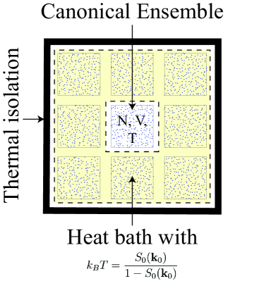
Figure 1: When a large number of systems can exchange heat with each other but not with the environment, one can focus on one system (central one indicated with a white background) and treat the rest as a heat bath (systems having yellow background). The central system with fixed $N$, $V$ and $T$ follows the distribution function of a classical canonical ensemble with a temperature $T$ determined by the total energy of the systems and degeneracy of the heat bath. For the problem at hand, we show that the temperature is determined by the target structure factor $S_{0}({\bf k})$, as specified by the relation $k_{B}T=S_{0}(\mathbf{q})/[1-S_{0}(\mathbf{q})]$.

The probability density function (PDF) of the total energy of any system in the canonical ensemble is given by

$$P(E)=\frac{g(E)\exp(-E/k_{B}T)}{Z},$$ (22)

where $Z$ is the partition function, $g(E)$ is energy degeneracy or density of states, and $T$ is the temperature. To determine the temperature of the heat bath explicitly in terms of $S_{0}(\mathbf{q})$, we make the simple observation that in the high-temperature or ideal-gas limit, the PDF (22) is proportional to the density of states

$$g(E)\propto\lim_{T\to\infty}P(E).$$ (23)

Thus, to determine the heat bath’s density of states and corresponding temperature for general correlated systems, we only need to know the distribution of its total energy, $E_{H}$, assuming the heat bath consists of $N_{c}-1$ uncorrelated (infinite-temperature) systems.

Let us first focus on one system comprising the heat bath, and denote its energy by $E_{1}$. For an ideal gas, each particle’s location is random and independent. Thus, for any particle $j$, $\exp(-i\mathbf{q}\cdot\mathbf{r}_{j})$ is a unit vector of a random orientation in the complex plane. Therefore, the collective density variable (17) is the sum of $N$ random unit vectors in the complex plane. From the theory of random walks, we know that for large $N$, ${\tilde{\rho}}(\mathbf{q})$ in the complex plane follows a Gaussian distribution, and the PDF of $|{\tilde{\rho}}(\mathbf{q})|$ is given by

$$P_{uncorr}(|{\tilde{\rho}}(\mathbf{q})|)=\frac{2|{\tilde{\rho}}(\mathbf{q})|}{N}\exp(-|{\tilde{\rho}}(\mathbf{q})|^{2}/N).$$ (24)

Therefore, the PDF of the energy $E_{1}=\mathcal{S}(\mathbf{q})=|{\tilde{\rho}}(\mathbf{q})|^{2}/N$ is given by

$$\begin{split}P_{uncorr}(E_{1})&=P_{uncorr}(|{\tilde{\rho}}(\mathbf{q})|)\left[\frac{d\mathcal{S}(\mathbf{q})}{d|{\tilde{\rho}}(\mathbf{q})|}\right]^{-1}\\ &=\exp(-E_{1}).\end{split}$$ (25)

Thus, the energy (i.e., the single-configuration structure factor) is exponentially distributed. This combined with (23) implies that the density of states of a single configuration is also an exponential function of the energy

$$g(E_{1})\propto\exp(-E_{1}).$$ (26)

For two uncorrelated configurations, the probability distribution of their total energy $E_{12}=E_{1}+E_{2}$ is

$$P_{uncorr}(E_{12}) =\int_{0}^{E_{12}}P_{uncorr}(E_{1})P_{uncorr}(E_{2})dE_{1}$$ (27)

$$=\int_{0}^{E_{12}}\exp(-E_{1})\exp\left[-(E_{12}-E_{1})\right]dE_{1}$$ (28)

$$=E_{12}\exp(-E_{12}).$$ (29)

The distribution for the total energy of three configurations is then

$$\begin{split}&P_{uncorr}(E_{123}=E_{12}+E_{3})\\ &=\int_{0}^{E_{123}}P_{uncorr}(E_{3})P_{uncorr}(E_{12})dE_{3}\\ &=\frac{E_{123}^{2}}{2}\exp(-E_{123}).\end{split}$$ (30)

Similarly, one can find that the distribution of the total energy of $N_{c}-1$ configuration is

$$P_{uncorr}(E=E_{1}+E_{2}+\cdots+E_{N_{c}-1})=\frac{E^{N_{c}-1}}{(N_{c}-1)!}\exp(-E).$$ (31)

As we detailed before, the density of states of the heat bath, made from $N_{c}-1$ systems, is proportional to the probability distribution function of the total energy of $N_{c}-1$ uncorrelated systems:

$$g(E)\propto P_{uncorr}(E)=\frac{E^{N_{c}-1}}{(N_{c}-1)!}\exp(-E).$$ (32)

The temperature of the heat bath is therefore

$$k_{B}T=\left[\frac{\partial\ln g(E)}{\partial E}\right]^{-1}=\left[\frac{N_{c}-1}{E}-1\right]^{-1},$$ (33)

where $E=E_{H}$ is the energy of the heat bath. On average, each configuration has an energy of $S_{0}(\mathbf{q})$. Therefore, in the $N_{c}\to\infty$ limit, $E_{H}=(N_{c}-1)S_{0}(\mathbf{q})$ and the heat-bath temperature is explicitly given by

$$k_{B}T=\frac{S_{0}(\mathbf{q})}{1-S_{0}(\mathbf{q})},$$ (34)

which is what we set out to prove.

In the $N_{c}\to\infty$ limit, the heat bath is infinitely large, and we can determine the probability density function of the energy of the reference system, $E_{R}$, which is not included in the heat bath, using the canonical distribution function, i.e.,

$$P(E_{R}) =\frac{g(E_{R})\exp(-E_{R}/k_{B}T)}{Z}$$ (35)

$$\propto\exp(-E_{R})\exp(-E_{R}/k_{B}T),$$ (36)

After normalization, one finds

$$P(E_{R})=\frac{\exp(-E_{R})\exp(-E_{R}/k_{B}T)}{S_{0}(\mathbf{q})}=\frac{\exp[-E_{R}/S_{0}(\mathbf{q})]}{S_{0}(\mathbf{q})}.$$ (37)

Since we previously defined $E_{R}=\mathcal{S}(\mathbf{q})$,

$$P[\mathcal{S}(\mathbf{q})]=\frac{\exp[-\mathcal{S}(\mathbf{q})/S_{0}(\mathbf{q})]}{S_{0}(\mathbf{q})}.$$ (38)

By symmetry, this distribution is applicable not only to the reference system, but also to the other $N_{c}-1$ systems as well. This means that for any particular configuration, its structure factor at a constrained $\mathbf{k}$ vector is exponentially distributed. We will numerically verify this conclusion in the Appendix. As in the ideal-gas case, the exponential distribution of $S(\mathbf{q})$ implies that ${\tilde{\rho}}(\mathbf{q})$ is Gaussian distributed.

As we previously showed, if one constrains the ensemble-averaged structure factor $S(\mathbf{q})$ to be equal to $S_{0}(\mathbf{q})$, the resulting configurations follow canonical-ensemble distribution of a system with energy defined as $E=\mathcal{S}(\mathbf{q})$ at temperature $k_{B}T=S_{0}(\mathbf{q})/(1-S_{0}(\mathbf{q}))$. Equivalently, one could also define a rescaled energy as

$$E={\tilde{v}}(\mathbf{q})\mathcal{S}(\mathbf{q}),$$ (39)

where

$${\tilde{v}}(\mathbf{q})=1/S_{0}(\mathbf{q})-1$$ (40)

and set $k_{B}T={\tilde{v}}(\mathbf{q})S_{0}(\mathbf{q})/(1-S_{0}(\mathbf{q}))=1$. As detailed in our earlier papers Fan et al. (1991); Uche et al. (2004); Torquato et al. (2015), such a definition of $E$ is equivalent to a pairwise additive potential. For example, in the thermodynamic limit, the total energy of such a system of particles with pairwise interactions is given by

$$E=\frac{\rho}{2}\int_{\mathbb{R}^{d}}v(\mathbf{r})g_{2}(\mathbf{r})d\mathbf{r},$$ (41)

which can be represented in Fourier space using Parseval’s theorem Torquato et al. (2015):

$$E=\frac{\rho}{2}{\tilde{v}}(\mathbf{k}=\mathbf{0})-\frac{1}{2}v(\mathbf{r}=\mathbf{0})+\frac{\rho}{2(2\pi)^{d}}\int_{\mathbb{R}^{d}}{\tilde{v}}(\mathbf{k})S(\mathbf{k})d\mathbf{k}.$$ (42)

The derivation of (39) and (40) applies to the cases where one constrains $S(\mathbf{k})$ at a single $\mathbf{k}$ vector. Can one generalize it to constraining $S(\mathbf{k})$ at multiple $\mathbf{k}$ vectors? If one constrains $S(\mathbf{k})$ at up to $d$ different orthogonal wave vectors (inner product being zero), formulas (39) and (40) would still apply exactly. This is because such constraints affect particle positions in different, independent directions, and can thus be treated separately. If the $d$ wave vectors are linearly independent but not orthogonal, one could still apply a linear transformation to reduce the problem to the orthogonal case.

To treat cases where the number of $\mathbf{k}$ vectors is larger than $d$, we recall that in Gibbs formalism, the inverse temperature is a Lagrange multiplier of energy. For multiple constrained wave vectors, $\mathbf{k}_{1}$, $\mathbf{k}_{2}$, $\cdots,\mathbf{k}_{N_{k}}$, we can use a separate Lagrange multiplier for each constraint. Consider maximizing the Gibbs entropy of the reference configuration

$$\mathscr{S}=-k_{B}\int P(\mathbf{r}^{N})\ln P(\mathbf{r}^{N})d\mathbf{r}^{N},$$ (43)

where $P(\mathbf{r}^{N})$ is the probability density function of the reference configuration, subject to constraints

$$C_{\mathbf{k}}=\int P(\mathbf{r}^{N})\mathcal{S}(\mathbf{k})d\mathbf{r}^{N}-S_{0}(\mathbf{k})=0$$ (44)

for each constrained $\mathbf{k}$, and

$$D=\int P(\mathbf{r}^{N})d\mathbf{r}^{N}-1=0,$$ (45)

If these constraints are satisfiable, we can find $P(\mathbf{r}^{N})$ by constructing the Lagrangian function

$$L=\mathscr{S}-\sum_{\mathbf{k}}\lambda_{\mathbf{k}}C_{\mathbf{k}}-\lambda_{D}D,$$ (46)

where $\lambda_{\mathbf{k}}$ and $\lambda_{D}$ are Lagrange multipliers. Setting $\delta L/\delta P(\mathbf{r}^{N})=0$, we find

$$P(\mathbf{r}^{N})=\frac{1}{Z}\exp\left[-\sum_{\mathbf{k}}\lambda_{\mathbf{k}}\mathcal{S}(\mathbf{k})\right],$$ (47)

where $Z=\int\exp\left[-\sum_{\mathbf{k}}\lambda_{\mathbf{k}}\mathcal{S}(\mathbf{k}_{j})\right]d\mathbf{r}^{N}$ is the partition function of the reference system. We see that if we define the fictitious energy as

$$E=\sum_{\mathbf{k}}\lambda_{\mathbf{k}}\mathcal{S}(\mathbf{k}),$$ (48)

which is still a pair potential Fan et al. (1991); Uche et al. (2004); Torquato et al. (2015), then $P(\mathbf{r}^{N})$ follows the equilibrium distribution at $k_{B}T=1$. However, we could not find an explicit expression for $\lambda_{\mathbf{k}}$. Theoretically, $\lambda_{\mathbf{k}}$ is completely determined by the target structure factor. However, the dependency is nontrivial due to the correlation between $S(\mathbf{k})$ at different $\mathbf{k}$ vectors. We proved that $S(\mathbf{k})$ is exponentially distributed in the single-constraint or independent-constraint cases. While we cannot prove that when multiple non-independent wave vectors are constrained, we do provide numerical evidence for such behavior in Appendix A.

To summarize, we have proved that if one constrains the ensemble-averaged structure factor at one or multiple $\mathbf{k}$ vectors, and if the constraints are satisfiable, then the resulting configurations are drawn from the canonical ensemble with a pairwise additive interaction (39) or (48). Thus, when we constrain $S(\mathbf{k})$ for all $\mathbf{k}$ vectors to be equal to a structure factor realized by some $n$-body interactions, our method finds an effective pair interaction that mimics the configurations produced by such $n$-body interactions. For the single-constraint case, we showed that the structure factor for a single configuration at the constrained $\mathbf{k}$ vector is exponentially distributed. For the multiple-constraint case, we will also show strong numerical evidence in Appendix A that the exponential distribution still holds. If the structure factor at the constrained $\mathbf{k}$ vectors are independent from one another, then the interaction is given by Eqs. (39)-(40), and the temperature is $k_{B}T=1$. However, if the structure factor at these $\mathbf{k}$ vectors are correlated, then (40) is inexact. We numerically test and verify these conclusions in Appendix A for specific examples.

II.3 Ensemble-Average Algorithm

Based on this theoretical formalism, we can now straightforwardly devise a new algorithm to construct a canonical ensemble of a finite but large number of configurations, $N_{c}$, targeting a particular functional form for the structure factor. Specifically, we minimize the squared difference for $N_{c}$ configurations but simultaneously, i.e.,

$$\mbox{minimize }\Phi(\mathbf{r}^{\cal{N}})=\sum_{\mathbf{k}\in\mathbb{K}}[\langle\mathcal{S}(\mathbf{k})\rangle-S_{0}(\mathbf{k})]^{2},$$ (49)

where ${\cal N}=NN_{c}$. Thus, compared to the standard collective-coordinate procedure Uche et al. (2006b); Batten et al. (2008); Zachary and Torquato (2011); Zhang et al. (2016), which has available $dN$ number of degrees of freedom, the canonical-ensemble-average generalization, enables us to substantially increase the number of degrees of freedom to $dNN_{c}$. Thus, in practice, the range of wave vectors over which we can constrain the structure factor to have a prescribed functional form can be made to be larger and larger by increasing the number of configurations.

Our algorithm involves minimizing a target function that is a sum over all $\mathbf{k}$ vectors within a wavenumber $K$ from the origin. The number of such $\mathbf{k}$ vectors scales as $K^{d}V$, where $V=N/\rho$ is the volume of the system. For each such $\mathbf{k}$ vector, we need to calculate $N_{c}$ structure factor values, each involves a summation over $N$ particles. Thus, the computational cost scales as $K^{d}VNN_{c}=K^{d}\rho^{-1}N^{2}N_{c}$. As $N$ grows, the computational cost grows quadratically and can become very large. However, the calculations for different $\mathbf{k}$ vectors can be carried out in parallel, and we can thus employ multiple GPUs to overcome the high computational cost. GPUs generally perform single-precision calculations faster than double-precision calculations, but we discovered that double precision is necessary for large system sizes ($N>1000$).

For cases in which $N>2000$, we found that the number of iterations needed to minimize the target function becomes computationally costly. By inspecting the intermediate configurations during minimization, we discovered that $S(\mathbf{k})$ near the origin ($\mathbf{k}=\mathbf{0}$) converges to $S_{0}(\mathbf{k})$ at much slower rate than that of $S(\mathbf{k})$ at other wave vectors. It is reasonable to assume that this slow-up is caused by the fact that changing $S(\mathbf{k})$ at $\mathbf{k}\approx\mathbf{0}$ requires long-range particle motions. To improve the convergence speed for small $k$ when $N>2000$, we introduce a weight of $w(k)=1/k$ in the previous objective function and then carry out the following minimization:

$$\mbox{minimize }\Phi(\mathbf{r}^{\cal{N}})=\sum_{\mathbf{k}\in\mathbb{K}}w(k)[\langle\mathcal{S}(\mathbf{k})\rangle-S_{0}(\mathbf{k})]^{2},$$ (50)

As a proof of concept of these modifications, we were able to generate $N_{c}=100$ configurations, each consisting of $N=20000$ particles, targeting the 1D fermionic target structure factor (58), after five days of computation using four NVIDIA Tesla P100 GPUs, as reported in Sec. III.1. Minimizing the objective function usually requires $\sim 10^{4}$ iterations in 1D but only $10^{2}-10^{3}$ iterations in 2D and 3D. Thus, we can generate higher-dimensional configurations with $N=20000$ particles much faster (about 30 times faster with our hardware).

In subsequent sections, we present results using $N_{c}=100$, which is large but still computationally manageable. Unless otherwise stated, each configuration consists of $N=400$ particles in a linear (1D), square(2D), or cubic (3D) simulation boxes with periodic boundary conditions. As we will show in Fig. 3, $N=400$ is large enough to produce pair statistics indistinguishable from $N=20000$ ones. The pair statistics are averaged over $5000$ configurations to reduce statistical fluctuations. Since the weight $w(k)=1/k$ is necessary only for sufficiently large configurations ($N>2000$), we omit it for simplicity. The set $\mathbb{K}$ contain half of all $\mathbf{k}$ vectors such that $0<|\mathbf{k}|<K$, where $K$ is a constant cutoff. We can omit one half of the $\mathbf{k}$ vectors within the range due to the inversion symmetry of the structure factor: $S(-\mathbf{k})=S(\mathbf{k})$. Unless otherwise stated, we use $K=30$ in 1D and $K=15$ in 2D and 3D. We use the low-storage BFGS algorithm Nocedal (1980); Liu and Nocedal (1989); Johnson to minimize $\Phi$, starting from random initial configurations. After the minimization, $\Phi$ is on the order of $10^{-4}-10^{-6}$. Considering that $\Phi$ is a sum over contributions from $N_{k}=10^{3}-10^{4}$ wave vectors, the difference between $S(\mathbf{k})$ and $S_{0}(\mathbf{k})$ at a particular wave vector is about $\sqrt{\Phi/N_{k}}=10^{-3.5}-10^{-5}$. The efficiency and accuracy of this algorithm is verified by applying to a variety of target structure factors described in Secs. III-VII. We present justifications of this algorithm and parameter choices in Appendix A.

III Proof of Concept: Targeting known realizable $S(k)$

As a proof-of-concept, we test our ensemble-average algorithm here by targeting several different structure factor functions across dimensions that are known to be exactly realizable. All of these examples are special cases of determinantal point processes, which are those whose $n$-point correlation functions are completely characterized by the determinant of some function Soshnikov (2000); Mehta (2004); Costin and Lebowitz (2004); Torquato et al. (2008); Hough et al. (2009).

III.1 Dyson’s One-Dimensional Log Coulomb Gases

Figure 2: (a): The structure factor obtained by sampling ensembles of 1D configurations in which the target function $S_{0}(k)$ is taken to be Eq. (54) at $\rho=1$. (b): The corresponding pair correlation function sampled from simulations and the analytical formula (63). Here it turns out that our usual reciprocal-space cutoff of $K=30$ is not large enough, and so we use $K=50$ instead.

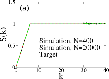
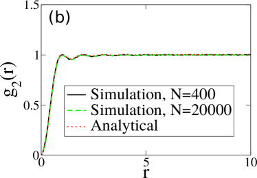
Figure 3: (a): The structure factor obtained by sampling ensembles of 1D configurations in which the target function $S_{0}(k)$ is taken to be Eq. (58) at $\rho=1$. We use two different system sizes, and show here that their pair statistics are indistinguishable. For $N=20000$, we generate 100 configurations instead of the usual 5000 configurations. (b): The corresponding pair correlation function sampled from simulations and the analytical formula (64).

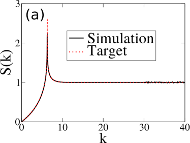
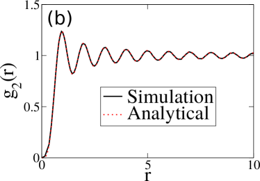
Figure 4: (a): The structure factor obtained by sampling ensembles of 1D configurations in which the target function $S_{0}(k)$ is taken to be Eq. (62) at $\rho=1$. (b): The corresponding pair correlation function sampled from simulations and the analytical formula (65).

Circular ensembles in the theory of random matrices Mehta (2004) are measures on spaces of unitary matrices introduced by Dyson as modifications of Gaussian matrix ensembles. These different ensembles are equivalent to one another when the matrix size tends to infinity. Dyson showed that the distribution of eigenvalues can be mapped to systems of particles on a circle interacting with a two-dimensional Coulomb potential (logarithmic function) at positive temperatures. These systems in turn can be mapped to logarithmically interacting particles in $\mathbb{R}$ with an appropriately confining potential.

The structure factors that correspond to those of the circular orthogonal ensemble (COE), circular unitary ensemble (CUE), and circular symplectic ensemble (CSE), respectively Mehta (2004); Torquato et al. (2008); Scardicchio et al. (2009); Forrester (2016) at unit density ($\rho=1$) in the thermodynamic limit are:

$$S(k)=\left\{\begin{array}[]{lr}{\displaystyle\frac{k}{\pi}-\frac{k}{2\pi}\ln(k/\pi+1)},\quad 0\leq k\leq 2\pi\\ \\ \displaystyle{2-\frac{k}{2\pi}\ln\left(\frac{k/\pi+1}{k/\pi-1}\right)},\quad k>2\pi,\end{array}\right.$$ (54)

$$S(k)=\left\{\begin{array}[]{lr}{\displaystyle\frac{k}{2\pi}},\quad 0\leq k\leq 2\pi\\ \\ \displaystyle{1},\quad k>2\pi,\end{array}\right.$$ (58)

and

$$S(k)=\left\{\begin{array}[]{lr}{\displaystyle\frac{k}{4\pi}-\frac{k}{8\pi}\ln\Big{|}1-k/(2\pi)\Big{|}},\quad 0\leq k\leq 4\pi\\ \\ \displaystyle{1},\quad k>4\pi.\end{array}\right.$$ (62)

These ensembles correspond to the following values of the inverse temperature $\beta=(k_{B}T)^{-1}$: $\beta=1$ (COE), $\beta=2$ (CUE), and $\beta=4$ (CSE). In all cases, we see that the structure factor $S(k)$ tends to zero linearly in $k$ in the limit $k\to 0$ and hence, according to (10) and (14), are hyperuniform of class II Torquato (2018). The case $\beta=2$ has been generalized to higher dimensions (detailed below) and found to possess identical distribution with a spin-polarized fermionic system Torquato et al. (2008).

The corresponding pair correlations of the COE, CUE and CSE are respectively

$$\begin{split}g_{2}(r)=&1-\frac{\sin^{2}(\pi r)}{(\pi r)^{2}}\\ &+\frac{\Big{(}\pi r\cos(\pi r)-\sin(\pi r)\Big{)}\Big{(}2\,\mbox{Si}(\pi r)-\pi\Big{)}}{2(\pi r)^{2}},\ \end{split}$$ (63)

$$g_{2}(r)=1-\frac{\sin^{2}(\pi r)}{(\pi r)^{2}},$$ (64)

and

$$\begin{split}g_{2}(r)=&1-\frac{\sin^{2}(2\pi r)}{(2\pi r)^{2}}\\ &+\frac{\Big{(}2\pi r\cos(2\pi r)-\sin(2\pi r)\Big{)}\,\mbox{Si}(2\pi r)}{4(\pi r)^{2}},\end{split}$$ (65)

We now apply our algorithm by targeting these three structure factors for systems with $N=400$. The target analytical forms for the structure factor for $\beta=1$, $\beta=2$, and $\beta=4$ and the corresponding simulation data are plotted in Figs.  2,  3,  and  4, respectively. We include in these figures the corresponding pair correlation functions, both the analytical forms and the simulation data, as obtained by sampling the generated configurations. From all of these figures, we see that our targeting algorithm enables us to realize these ensembles with high accuracy, validating its utility and applicability. For the $\beta=2$ case, we also carried out the simulation results for a much larger system with $N=20,000$. We see from Fig. 3 that the results for $N=400$ are indistinguishable from those for $N=20000$.

By a theorem of Henderson Henderson (1974), a pair potential that gives rise to a given pair correlation function is unique up to a constant shift, although this cannot apply at $T=0$ foo ; Cohn and Kumar (2007); Cohn et al. (2019). The fact that our methodology yields ensembles of configurations with targeted pair statistics (whenever realizable) that are determined by effective pair potentials means that those interactions in the case of Dyson’s one-dimensional COE, CUE and CSE must exactly be given by the two-dimensional Coulombic potential.

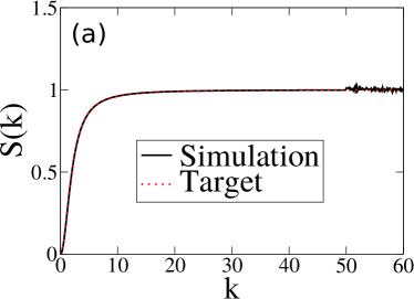
Figure 5: (a): The structure factor obtained by sampling ensembles of 1D configurations in which the target function $S_{0}(k)$ is taken to be Eq. (67) with $\lambda=2$ at $\rho=1$. (b): The corresponding pair correlation function sampled from simulations and the analytical formula as obtained from (66) [$g_{2}(r)=1-\exp(-2r)$]. Here it turns out that our usual reciprocal-space cutoff of $K=30$ is not large enough, and so we use $K=50$ instead.

III.2 One-dimensional Lorentzian target

Costin and Lebowitz Costin and Lebowitz (2004) showed that there exists a one-dimensional determinantal point process at unit density in which the total correlation function is the following simple exponential function:

$$h(r)=-\exp(-\lambda r),$$ (66)

where $\lambda\geq 2$. This corresponds to a structure factor with a Lorentzian form:

$$S(k)=\frac{\lambda(\lambda-2)+k^{2}}{k^{2}+\lambda^{2}}.$$ (67)

This result implies that the system is hyperuniform at the “borderline” case of $\lambda=2$, since the structure factor $S(k)=k^{2}/(4+k^{2})$ tends to zero quadratically in $k$ in the limit $k\to 0$ and hence, according to (10) and (14), are hyperuniform of class I Torquato (2018). We have targeted the $\lambda=2$ target, and successfully realize it. The results for the pair correlation function and the structure factor are presented in Fig. 5.

III.3 Fermi-sphere targets in higher dimensions

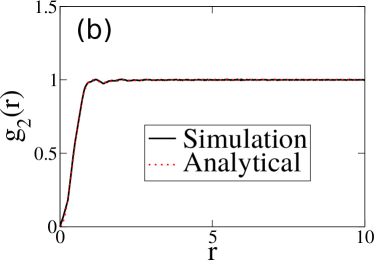
Figure 6: (a): The structure factor obtained by sampling ensembles of 2D configurations in which the target function $S_{0}(k)$ is taken to be Eq. (68) at $\rho=1$. (b): The corresponding pair correlation function sampled from simulations and the analytical formula (69).

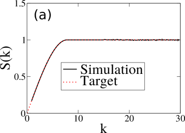
Figure 7: (a): The structure factor obtained by sampling ensembles of 3D configurations in which the target function $S_{0}(k)$ is taken to be Eq. (68) at $\rho=1$. (b): The corresponding pair correlation function sampled from simulations and the analytical formula (69).

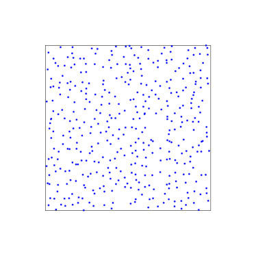
Figure 8: A two-dimensional, 400-particle “fermi-sphere” configuration drawn from ensembles in which the target function $S_{0}(k)$ is taken to be Eq. (68) at $\rho=1$.

The 1D CUE point process with a structure factor given by Eq. (58) has been generalized to so-called “Fermi-sphere” point processes in $d$-dimensional Euclidean space $\mathbb{R}^{d}$ Torquato et al. (2008). Specifically, such disordered hyperuniform point processes correspond to the spatial distribution of spin-polarized free fermions in $\mathbb{R}^{d}$, which are special cases of determinantal processes. In particular, the structure factor in $\mathbb{R}$ at unit density is given by

$$S(k)=1-\alpha(k,\kappa),$$ (68)

where $\alpha(k,\kappa)$ is the volume common to two spherical windows of radius $\kappa$ whose centers are separated by a distance $k$ divided by $v_{1}(\kappa)$, the volume of a spherical window of radius $\kappa=2\sqrt{\pi}[\Gamma(1+d/2)]^{1/d}$, which is known analytically in any dimension Torquato and Stillinger (2006a). This result implies that the structure factor $S(k)$ tends to zero linearly in $k$ in the limit $k\to 0$ and hence are hyperuniform of class II Torquato (2018). The corresponding pair correlation function of such a point process is given by

$$g_{2}(r)=1-2^{d}\Gamma(1+d/2)^{2}\frac{J^{2}_{d/2}(\kappa r)}{(\kappa r)^{d}},$$ (69)

where $J_{\nu}(x)$ is the Bessel function of the first kind of order $\nu$.

We have applied our algorithm to target the structure factor (68) in two and three dimensions using $K=15$. The results are presented in Figs. 6 and 7 along with the corresponding pair correlation functions sampled from the generated configurations as well as the analytical forms obtained from (69). Consistent with the known realizability of these targets, we see excellent agreement between the targeted structure factors and those obtained from our ensemble-average formulation. A two-dimensional configuration is shown in Fig. 8.

Unlike the one-dimensional COE, CUE, and CSE determinantal point configurations, the interaction potential for general determinantal point processes must contain at least up to three-body potentials; see the Appendix of Ref. Torquato et al., 2008. Thus, for the 2D and 3D fermi-sphere targets as well as the 1D Lorentzian target (Sec. III.2), we show for the first time that there exists effective pair interactions that mimic the higher-order $n$-body interactions corresponding to these determinantal point processes.

III.4 Gaussian target in two dimensions

An example of a 2D determinantal point process that exhibits hyperuniform behavior is generated by the Ginibre ensemble Jancovici (1981), which is a special case of the two-dimensional one-component plasma Jancovici (1981). A one-component plasma (OCP) is an equilibrium system of identical point particles of charge $e$ interacting via the log Coulomb potential and immersed in a rigid, uniform background of opposite charge to ensure overall charge neutrality. For $\beta=2$, the total correlation function for the OCP (Ginibre ensemble) in the thermodynamic limit was found exactly by Jancovici Jancovici (1981):

$$h(r)=-\exp\left(-\rho\pi r^{2}\right).$$ (70)

The corresponding structure factor is given by

$$S(k)=1-\exp\left(-\frac{k^{2}}{4\pi\rho}\right).$$ (71)

This result implies that the structure factor $S(k)$ tends to zero quadratically in $k$ in the limit $k\to 0$ and hence are hyperuniform of class II Torquato (2018).

Using our method, we targeted the OCP structure factor (71) using $K=15$. As shown in Fig. 9, it is seen that the algorithm is able to realize this target with very high accuracy. The corresponding pair correlation function obtained by sampling the resulting configurations agrees very well with the exact $g_{2}(r)$ obtained from (70), as shown in Fig. 9. One configuration is shown in Fig. 10. It it noteworthy that we had previously employed a completely different algorithm to generate these configurations as well as other determinantal point processes Scardicchio et al. (2009), but the maximum attainable system sizes were substantially much smaller ($N\approx 100$) in that study.

Figure 9: (a): The structure factor obtained by sampling ensembles of 2D configurations in which the target function $S_{0}(k)$ is taken to be Eq. (71) at $\rho=1$. (b): The corresponding pair correlation function sampled from simulations and the analytical formula (70).

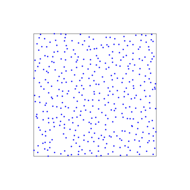
Figure 10: A two-dimensional, 400-particle OCP configuration drawn from ensembles in which the target function $S_{0}(k)$ is taken to be Eq. (71) at $\rho=1$.

IV Another proof of concept: Targeting a known unrealizable $S(k)$

A severe test of our algorithm and another proof of concept would be its application to hypothetical functional forms for pair statistics that meet the explicitly known necessary realizability conditions (1)-(3), i.e., nonnegativity conditions on $g_{2}(r)$ and $S(k)$ as well as the Yamada condition, but is known not be realizable. Such examples are rare. One particular two-dimensional example was identified by Torquato and Stillinger Torquato and Stillinger (2006a) in which the point configuration would putatively correspond to a packing of identical hard circular disks of unit diameter with a pair correlation function given by

$$g_{2}(r)=\Theta(r-\sigma)+\frac{Z}{2\pi\rho}\delta(r-1),$$ (72)

where $\Theta(x)$ is the unit step function, $\delta(r)$ is a radial Dirac delta function, $\sigma=1.2946$ and $Z=4.0148$. The corresponding structure is given by

$$S(k)=1-\frac{8\phi\sigma^{2}}{(k\sigma)}J_{1}(k\sigma)+ZJ_{0}(k),$$ (73)

where $\phi=0.74803$ is the packing fraction. It turns out that both $g_{2}(r)$ and $S(k)$ are nonnegative functions and the Yamada condition is satisfied. However, Torquato and Stillinger Torquato and Stillinger (2006a) observed that the test function (72) cannot correspond to a packing because it violates local geometric constraints specified by a distance $\sigma$ and average contact number (per particle) $Z$. Specifically, for $Z=4.0148$, there must be particles that are in contact with at least five others. But no arrangement of the five exists that is consistent with the assumed pair correlation function (step plus delta function with a gap from 1 to 1.2946).

We use our standard procedure described in Sec. II.3 to target the structure factor (73), but we change three parameters. We take $N_{c}=1000$ (rather than $N_{c}=100$) to ensure that any failure is not due to lacking degrees of freedom and use $N=100$ (rather than $N=400$) to compensate for the increase in simulation time caused by the previous change. Finally, we experimented with several values of $K$ values (shown in Fig. 11), instead of the standard usage of $K=15$ in 2D.

We present results for three different reciprocal-space cutoff values: $K=10,15,20$. For $K=10$, the structure factor can match the target inside the constrained region. Importantly, for the two larger $K$ values, the optimizer finds local minima, and the final structure factors (at the end of the minimization) does not match the target, even inside the constrained region. Therefore, we conclude that the structure factor (73) is not realizable, which speaks to the power of our algorithm.

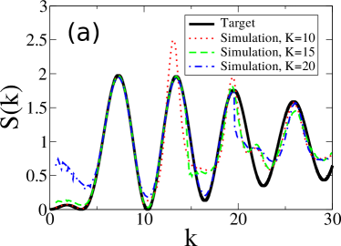
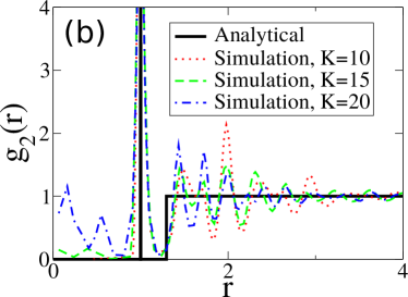
Figure 11: (a): The structure factor obtained by sampling ensembles of 1D configurations in which the target function $S_{0}(k)$ is taken to be Eq. (73) at $\rho=1$. (b): The corresponding pair correlation function sampled from simulations and the analytical formula (72).

V Targeting hyperuniform structure factors with unknown realizability

In this section, we apply our ensemble-average algorithm to target several different hyperuniform functional forms for structures factors across dimensions that satisfy the explicitly known necessary conditions (1)-(3), but are not known to be realizable. We show that all of these $d$-dimensional targets are indeed realizable.

Before presenting these results, it is instructive to comment on the effect of space dimensionality on realizing a prescribed structure factor. It is generally known that the lower the space dimension, the more difficult it is to satisfy realizability conditions Torquato and Stillinger (2006a). This is consistent with decorrelation principle Torquato and Stillinger (2006a), which states that unconstrained correlations in disordered many-particle systems vanish asymptotically in high dimensions and that the $n$-particle correlation function $g_{n}$ for any $n\geq 3$ can be inferred entirely from a knowledge of $\rho$ and $g_{2}$. This in turn implies that the nonnegativity of $g_{2}(r)$ and $S(k)$ are sufficient conditions for realizability. It was also shown that the decorrelation principle applies more generally to lattices in high dimensions Andreanov et al. (2016).

V.1 Gaussian Structure Factor Across Dimensions

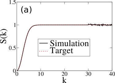
Figure 12: (a): The structure factor obtained by sampling ensembles of 1D configurations in which the target function $S_{0}(k)$ is taken to be Eq. (75) with $a=1/\sqrt{\pi}$ at $\rho=1$. (b): The corresponding pair correlation function sampled from simulations and the analytical formula (74).

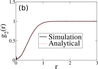
Figure 13: (a): The structure factor obtained by sampling ensembles of 3D configurations in which the target function $S_{0}(k)$ is taken to be Eq. (75) with $a=1/\sqrt{\pi}$ at $\rho=1$. (b): The corresponding pair correlation function sampled from simulations and the analytical formula (74). Here it turns out that our usual reciprocal-space cutoff of $K=15$ is not large enough, and so we use $K=25$ instead.

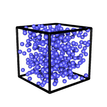
Figure 14: A three-dimensional, 400-particle configuration drawn from ensembles in which the target function $S_{0}(k)$ is taken to be Eq. (75) at $\rho=1$.

To begin, we ask whether a total correlation function with the following Gaussian form is realizable as a hyperuniform system across dimensions:

$$h(r)=-\exp\left(-(r/a)^{2}\right),$$ (74)

where $a$ is a positive constant. The corresponding structure factor is given by

$$S(k)=1-\rho a^{d}\pi^{d/2}\exp\left(-\frac{k^{2}}{4\pi\rho}\right),$$ (75)

which implies that $S(k)$ tends to zero quadratically as $k\to 0$ for all $d$. The hyperuniformity condition requires the unique density to be given by $\rho=(a\sqrt{\pi})^{-d}$. Note that the case $d=2$ is exactly the same as the two-dimensional OCP system in which $h(r)$ and $S(k)$ are given by (70) and (71), respectively.

We target such structure factors in one and three dimensions and find that they are realizable as hyperuniform systems at unit density. For $d=1$, we find excellent agreement between the simulated and target structure factors are obtained, as shown in Fig. 12. This strongly suggests that such systems are realizable in one dimension, the most difficult dimensionality case. Indeed, we also find the same excellent agreement between the simulated and target structure factors in three dimensions, as illustrated in Fig. 13. We conclude that such targets are realizable as disordered hyperuniform systems of class I Torquato (2018) in any space dimension whenever $\rho=(a\sqrt{\pi})^{-d}$. A 3D configuration is shown in Fig. 14.

V.2 $d$-dimensional generalization of the OCP pair correlation function

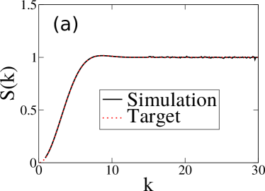
Figure 15: (a): The structure factor obtained by sampling ensembles of 3D configurations in which the target function $S_{0}(k)$ is taken to be Eq. (77) at $\rho=1$. (b): The corresponding pair correlation function sampled from simulations and the analytical formula (76).

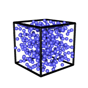
Figure 16: A three-dimensional, 400-particle configuration drawn from ensembles in which the target function $S_{0}(k)$ is taken to be Eq. (77) at $\rho=1$.

Consider the following $d$-dimensional generalization of the total correlation function of the OCP:

$$h(r)=-\exp[-\rho v_{1}(r)],$$ (76)

where $v_{1}(r)$ is the volume of a sphere of radius $r$ [cf. (4)]. It is noteworthy that such a total correlation function automatically satisfies the hyperuniformity requirement for any positive density and any $d$, since ${\tilde{h}}(k=0)=\int_{\mathbb{R^{d}}}h(r)d{\bf r}=-1/\rho$ [cf. (2) and (5)]. Note that when $d=1$, this is identical to the realizable total correlation function (66) with $\lambda=2\rho$. Moreover, when $d=2$, this is identical to the realizable OCP function (70).

It is not known whether configurations corresponding to (76) for $d\geq 3$ are realizable. We target the structure factor in this case in three dimensions:

$$\begin{split}S(k)=&1-\frac{1}{1080\rho^{4/3}\pi^{2/3}\Gamma(2/3)}\bigg{\{}\\ &2^{1/3}3^{5/6}\pi^{1/3}{}_{0}F_{3}\left[-;\frac{4}{3},\frac{3}{2},\frac{11}{6};a(k)\right]k^{4}\\ &-30(6\rho)^{2/3}\Gamma\left(\frac{2}{3}\right)^{2}{}_{0}F_{3}\left[-;\frac{2}{3},\frac{7}{6},\frac{3}{2};a(k)\right]k^{2}\\ &+1080\Gamma\left(\frac{2}{3}\right)\pi^{2/3}\rho^{4/3}{}_{1}F_{4}\left[1;\frac{1}{3},\frac{2}{3},\frac{5}{6},\frac{7}{6};a(k)\right]\bigg{\}},\end{split}$$ (77)

where $\Gamma(x)$ is the gamma function, ${}_{p}F_{q}(a_{1},\cdots,a_{p};b_{1},\cdots,b_{q};z)$ is the generalized hypergeometric function, and

$$a(k)=\frac{k^{6}}{20736\pi^{2}\rho^{2}}.$$ (78)

For small wavenumbers, this 3D structure factor as well as those for any other values of $d$ goes to zero quadratically in $k$ as $k$ tends to zero; specifically,

$$S(k)\sim k^{2}\qquad(k\to 0).$$ (79)

This means that $S(k)$ is analytic at the origin, which in turn implies that $h(r)$ decays to zero exponentially fast or faster Torquato (2018). We find that this 3D structure factor is indeed realizable for $\rho=1$. The results depicted in Fig. 15 show excellent agreement between the simulated and target structure factors. One such configuration is shown in Fig. 16. Since (76) is realizable for $d=3$, it should be realizable in higher dimensions and hence such systems in $\mathbb{R}^{d}$ for any $d$ are hyperuniform of class I Torquato (2018).

V.3 Fourier dual of relation (76)

Here we consider the Fourier dual of the function (76) in $d$ dimensions, namely,

$$\rho{\tilde{h}}(k)=-\exp[-v_{1}(k)/(2\pi)^{d}\rho],$$ (80)

which implies

$$S(k)=1-\exp[-v_{1}(k)/(2\pi)^{d}\rho].$$ (81)

Thus, the structure factor has the following asymptotic power-law behavior for any $d$:

$$S(k)\sim k^{d}\qquad(k\to 0).$$ (82)

The realizability of such structure factors, which would be hyperuniform for any density and $d$, has heretofore not been studied in any space dimension, except for $d=2$, where it has the same form as the OCP structure factor (71). It is crucial to note that unlike the structure factor corresponding to (76), which is analytic at the origin [cf. (79)], the structure factor (81) is nonanalytic at the origin for any odd dimension. This attribute in odd dimensions results in pair correlation functions that for large $r$ are controlled by a power-law decay $1/r^{2d}$; see Ref. Torquato (2018) for a general analysis of such asymptotics. The corresponding total correlation functions in the first three space dimensions are given respectively by

$$h(r)=\frac{-1}{(\pi\rho r)^{2}+1},$$ (83)

$$h(r)=-\exp(-\pi\rho r^{2}),$$ (84)

$$h(r)=f(r)-1,$$ (85)

where

$$f(r)=S(k=2\pi\rho^{2/3}r)$$ (86)

and $S(k)$ is the structure factor for the 3D generalization of OCP, given in Eq. (77).

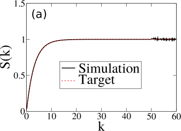
Figure 17: (a): The structure factor obtained by sampling ensembles of 1D configurations in which the target function $S_{0}(k)$ is taken to be Eq. (81) at $\rho=1$. (b): The corresponding pair correlation function sampled from simulations and the analytical formula (83). Here it turns out that our usual reciprocal-space cutoff of $K=30$ is not large enough, and so we use $K=50$ instead.

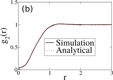
Figure 18: (a): The structure factor obtained by sampling ensembles of 3D configurations in which the target function $S_{0}(k)$ is taken to be Eq. (81) at $\rho=1$. (b): The corresponding pair correlation function sampled from simulations and the analytical formula (85).

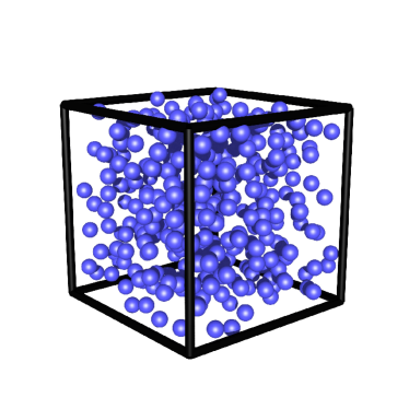
Figure 19: A three-dimensional, 400-particle configuration drawn from ensembles in which the target function $S_{0}(k)$ is taken to be Eq. (81) at $\rho=1$.

We target such structure factors in one and three dimensions and find that they are realizable as hyperuniform systems at unit density. Excellent agreement between the simulated and target structure factors are obtained, as shown in Figs. 17 and 18. A three-dimensional configuration is shown in Fig. 19. For aforementioned reasons, this means that the function (81) is realizable for higher dimensions ($d\geq 4$) and hence for all positive dimensions. Therefore, we see from (10), (14) and (82) that such systems are hyperuniform of class II for $d=1$ and of class I for $d\geq 2$.

VI Targeting nonhyperuniform structure factors with unknown realizability

In this section, we apply our ensemble-average algorithm to target two different nonhyperuniform functional forms for the structure factor in 2D and 3D. As before, they both satisfy the explicitly known necessary conditions (1)-(3), but are not known to be realizable. We show that all of these targets are indeed realizable.

VI.1 Hyposurficial structure factors in two and three dimensions

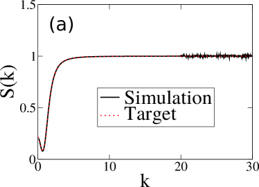
Figure 20: (a): The structure factor obtained by sampling ensembles of 2D configurations, in which the target function $S_{0}(k)$ is numerically computed from Eq. (2) and (87), at $\rho=0.5$. (b): The corresponding pair correlation function sampled from simulations and the analytical formula (87).

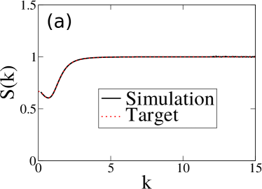
Figure 21: (a): The structure factor obtained by sampling ensembles of 3D configurations, in which the target function $S_{0}(k)$ is taken to be Eq. (89), at $\rho=\frac{1}{4\pi}$. (b): The corresponding pair correlation function sampled from simulations and the analytical formula (88).

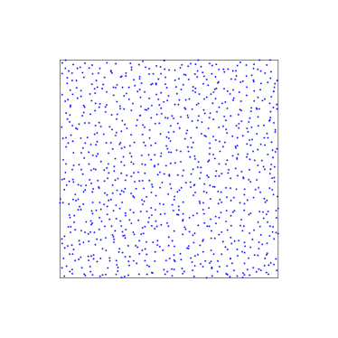
Figure 22: A two-dimensional, 1000-particle hyposurficial configuration drawn from ensembles in which the target function $S_{0}(k)$ is numerically computed from Eq. (2) and (87), at $\rho=0.5$.

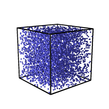
Figure 23: A three-dimensional, 4000-particle hyposurficial configuration drawn from ensembles in which the target function $S_{0}(k)$ is taken to be Eq. (89) at $\rho=\frac{1}{4\pi}$.

As we have discussed in the introduction, a hyposurficial state of matter has $A>0$ and $B=0$ in Eq. (6). Hyposurficiality may be considered the opposite of hyperuniformity because the latter implies $A=0$ and $B>0$. Although there is numerical evidence of $B$ vanishing at a particular pressure in a model amorphous ice martelli2017large , a rigorous proof of the existence of hyposurficial point configurations has heretofore not been found.

Here we design and realize hyposurficial structure factors in 2D and 3D. Since $B$ is proportional to the $d$-th moment of $h(r)$ [see Eq. (8)], we designed the following well-behaved hyposurficial $h(r)$ targets

$$h(r)=\frac{\exp(-r)}{4}-\frac{\exp(-r)\sin(r)}{r},$$ (87)

$$h(r)=\frac{\exp(-r)}{4\pi}-\frac{\exp(-r)\sin(r)}{r},$$ (88)

in 2D and 3D respectively. We choose realizable densities $\rho=\frac{1}{2}$ in 2D and $\rho=\frac{1}{4\pi}$ in 3D. The 3D target can be analytically transformed into an $S(k)$ target

$$S(k)=\frac{6k^{8}+12k^{6}+19k^{4}+24k^{2}+16}{6(k^{2}+1)^{2}(k^{2}-2k+2)(k^{2}+2k+2)}$$ (89)

but the 2D $h(r)$ target has no corresponding analytical $S(k)$. We target a numerically obtained tabulated $S(k)$ instead.

We have successfully realized these targets with tuned parameters: $N=1000$, $N_{c}=200$, and $K=20$ in 2D; and $N=4000$, $N_{c}=1000$, and $K=12$ in 3D. We increase the system size $N$ because in both cases, $S(k)$ possesses a small kink near the origin, and we need large systems to access smaller $k$ values. Our success in realizing these targets demonstrates, for the first time, that hyposurficial point configurations indeed exist.

Reference martelli2017large, observed that hyposurficiality appears to be associated with spacial heterogeneities, and so it is interesting to see if our configurations also exhibit such characteristics. We present these configurations in Figs. 22 and 23, which indeed show spatial heterogeneities that are manifested by significant clustering of the particles.

VI.2 Antihyperuniform structure factors in two dimensions

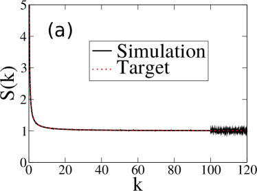
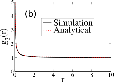
Figure 24: (a): The structure factor obtained by sampling ensembles of 2D configurations, in which the target function $S_{0}(k)$ is taken to be Eq. (90) at $\rho=1$ and $\kappa=0$. (b): The corresponding pair correlation function sampled from simulations and the analytical formula (91).

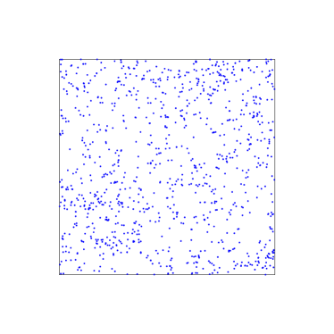
Figure 25: A two-dimensional, 1000-particle antihyperuniform configuration drawn from ensembles in which the target function $S_{0}(k)$ is taken to be Eq. (90) at $\rho=1$ and $\kappa=0$.

As discussed in the Introduction, an antihyperuniform configuration is one for which $S(k)$ diverges at $k=0$. Although this behavior has been observed at various critical points, it is still interesting to challenge our algorithm to generate such configurations. We designed the following target structure factor in 2D:

$$S(k)=1+\frac{1}{\sqrt{k^{2}+\kappa^{2}}}.$$ (90)

Such a system, if realizable, would achieve antihyperuniformity at $\kappa=0$. The corresponding pair correlation function is

$$g_{2}(r)=1+\frac{\exp(-\kappa r)}{2\pi r}.$$ (91)

We have indeed successfully realized this target at $\rho=1$, $\kappa=0$, 0.3, and 1. We show the antihyperuniform case, $\kappa=0$, in Figs. 24 and 25. In realizing this target, we used parameters $N=1000$, $N_{c}=3000$, and $K=100$. We use a large value of $N$ to provide sufficient resolution to determine $S(k)$ at small $k$, and an extremely large value of $K$, since this target $S_{0}(k)$ decays very slowly to unity as $k$ increases. Since $K$ is large, we also need a sufficiently large value of $N_{c}$ to provide ample degrees of freedom.

VII Conjecture regarding the realizability of equilibrium and nonequilibrium configurations via effective pair interactions

Our equilibrium ensemble-average formalism to solve the realizability problem in $\mathbb{R}^{d}$ raises a profound fundamental theoretical question: Can any realizable $g_{2}({\bf r})$ or $S({\bf k})$ associated with either an equlibriium or nonequilibrium ensemble be attained by an equilibrium systems with effective pairwise interaction? Currently, there is no rigorous proof that the answer to this question is in the affirmative in the implied thermodynamic limit. However, there are sound arguments and reasons to conjecture that such an effective pair interaction can always be found, perhaps under some mild conditions. First, our theoretical formalism strongly supports this conjecture, since it exploits the fact that an equilibrium ensemble of configurations in $\mathbb{R}^{d}$ offers an infinite number of degrees of freedom to attain a realizable $g_{2}({\bf r})$ or, equivalently, $S({\bf k})$ in the thermodynamic limit with an associated pair potential $v({\bf r})$ at positive temperatures. While our procedure is not suited for ground states ($T=0$), such targeted structures are even easier to achieve by pair interactions in light of the high degeneracy of pair potentials consistent with a ground-state structure foo . Second, for finite-sized systems of particles that are restricted to lie on lattice sites in $\mathbb{R}^{d}$, it has been proved, under rather general conditions, that any realizable $g_{2}({\bf r})$ can be achieved by a pair potential $v({\bf r})$ at positive temperatures Kuna et al. (2011). Third, the success of our algorithm in all of the known realizable targets cases with nonadditive interactions supports this conjecture, even if the simulations were necessarily carried out on finite systems under periodic boundary conditions.

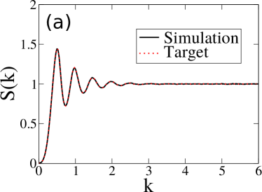
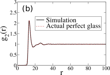
Figure 26: (a): The structure factor obtained by sampling ensembles of 2D configurations in which the target function $S_{0}(k)$ is taken to be equal to the numerically measured $S(k)$ of a perfect-glass system at $\rho=0.00390625$. (b): The corresponding pair correlation function sampled from targeted configurations, compared with that of an actual perfect glass.

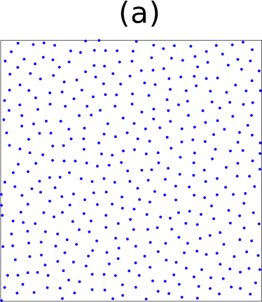
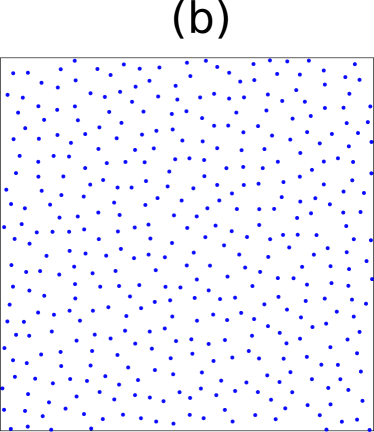
Figure 27: (a): A two-dimensional configuration of 400 particles drawn from ensembles in which the target function $S_{0}(k)$ is taken to be equal to the numerically measured $S(k)$ of a perfect-glass system at $\rho=0.00390625$. (b): An actual perfect-glass configuration with the same pair statistics $g_{2}(r)$ and $S(k)$.

As a highly stringent test of our affirmative answer, we now target nonequilibrium “perfect-glass” structure factors Zhang et al. (2016), which are glassy, nonequilibrium state of a many-particle system interacting with two-, three-, and four-body potentials. Counterintuitively, the classical ground state of this many-body interaction is unique and disordered zhang2017classical . By construction, it banishes crystals and quasicrystals from the ground-state manifold. We have previously investigated the quenched states from infinite temperature to zero temperature for this model with various parameter choices, and numerically computed their structure factors. Here we target the numerically-measured structure factor of a perfect glass model with parameters $d=2$, $\rho=0.00390625$, $\chi=5.10$, $\alpha=2$, and $\gamma=3$ (see Ref. Zhang et al., 2016 for the definition of the last three parameters). We use targeting parameters $N_{c}=1000$ and $K=5$. This seemingly small value of $K$ is actually relatively large considering that $\rho$ is much smaller than unity, since real-space length scale is inversely proportional to the $k$-space length scale. Figures 26 shows the excellent agreement between the targeted and simulated structure factors and pair correlation functions. This is a remarkable suggestion that the answer to our question above is affirmative because a perfect glass is a nonequilibrium system with two-, three-, and four-body interactions while our reconstructed system is an equilibrium state of a pair potential.

It is interesting to compare configurations produced by the actual perfect glass interaction and the effective pair interaction visually, as is done in Fig. 27. Although these pair of configurations look strikingly similar to one another, we know that since one system involves three- and four-body interactions and the other does not, that their higher-order statistics ($g_{3}$, $g_{4}$, $\cdots$) must be different Torquato and Stillinger (2006a); Jiao et al. (2010); stillinger2019structural , even if such distinctions cannot be detected visually.

The realizability of a perfect glass using our formalism as well as the findings reported in Secs. III-VI lead us to the following conjecture:

Given the pair correlation function $g_{2}({\bf r})$ of any realizable statistically homogeneous many-particle ensemble (equilibrium or not) in $\mathbb{R}^{d}$ at number density $\rho$, there is an equilibrium ensemble (Gibbs measure) involving only an effective pair potential $v({\bf r})$ that gives rise to such a $g_{2}({\bf r})$.

Note that statistical homogeneity implies that thermodynamic limit has been taken. The rigorous validity of this conjecture is an outstanding open problem.

VIII Conclusions and Discussion

To address the realizability problem, we introduced a theoretical formalism that provides a means to draw disordered particle configurations at positive temperatures from canonical ensembles with certain pairwise-additive potentials that could correspond to disordered targeted analytical functional forms for the structure factor. This theoretical foundation enabled us to devise an efficient algorithm to construct systematically canonical-ensemble particle configurations with such targeted pair statistics whenever realizable. As a proof-of-concept, we tested this algorithm to target several different structure factor functions across dimensions that are known to be realizable and one hyperuniform target that meets all explicitly known necessary realizability conditions but is known to be nontrivially unrealizable. Our algorithm succeeded for all realizable targets and appropriately failed for the unrealizable target, demonstrating the accuracy and power of the method to numerically investigate the realizability problem. Having established the prowess of the methodology, we targeted several families of structure-factor functions that meet the known necessary realizability conditions but were heretofore not known to be realizable, including $d$-dimensional Gaussian structure factors, $d$-dimensional generalizations of the 2D one-component plasma, the $d$-dimensional Fourier duals of the previous OCP cases, a hyposurficial target in 2D and 3D, and an antihyperuniform target in 2D. In all of these instances, we were able to achieve the targeted structure factors with high accuracy, suggesting that these targets are indeed truly realizable by equilibrium many-particle systems with pair interactions at positive temperatures. This expands our knowledge of analytical functional forms for $g_{2}(r)$ and $S(k)$ associated with disordered point configurations across dimensions. When targeting hyposurficial structure factors, we confirm a previous observation that hyposurficiality is associated with spatial heterogeneities that are manifested by significant clustering of the particles martelli2017large . Our results, especially perfect-glass realizability, led to the conjecture that any realizable structure factor corresponding to either an equilibrium or nonequilibrium system can be attained by an equilibrium ensemble involving only effective pair interactions in the thermodynamic limit.

It is worth stressing that we only constrain $S(k)$ in a finite range ($0<|k|<K$) numerically for $K$ as large as feasibly possible, but do not enforce explicit constraints on $g_{2}(r)$. Since $g_{2}(r)$ for small $r$ is related to $S(k)$ for large $k$, there is no guarantee that the numerically sampled $g_{2}(r)$ matches its analytical counterpart at very small pair distances (i.e., $r<2\pi/K$). Nevertheless, we always find impressive consistency between the simulated and analytical pair correlation functions corresponding to the target $S(k)$, which further demonstrates the success of our algorithm.

Realizable particle configurations generated with a targeted pair correlation function using our algorithm are equilibrium states of pairwise additive interactions at positive temperatures. Such a pair potential is unique up to a constant shift Henderson (1974). In the case of realizable hyperuniform targets with the smooth pair correlation functions considered here, such interactions must be long-ranged Torquato (2018), which is a consequence of the well-known fluctuation-compressibility relation:

$$\lim_{k\to 0}S(k)=\rho k_{B}T\kappa_{T},$$ (92)

where $\kappa_{T}$ is the isothermal compressibility. Since $\lim_{k\to 0}S(k)=0$ and $\rho k_{B}T>0$, one must have $\kappa_{T}=0$. Using the analysis that relates the large-$r$ behavior of the direct correlation function to that of the pair potential function $v(r)$ presented in Ref. Torquato, 2018, it immediately follows that the asymptotic behavior of $v(r)$ is Coulombic for the Gaussian S(k) [cf. (47)] for $d\geq 3$, i.e.,

$$\beta v(r)\sim 1/r^{d-2}\qquad r\to\infty,$$ (93)

which, of course, is a long-ranged interaction. The same asymptotic Coulombic form for the pair potential for $d\geq 3$ arises in the $d$-dimensional generalization of the OCP pair correlation function (76). It would be an interesting future research direction to find the specific functional forms of such pair interactions. For general determinantal point processes, these would be effective pair interactions that mimic the two-body, three-body, and higher-order intrinsic interactions Torquato et al. (2008).

Our study is also a step forward in being able to devise inverse methods torquato2009inverse ; zhang2013probing to design materials with desirable physical properties that can be tuned by their pair statistics. Pair statistics combined with effective pair interactions, which in principle can be obtained using inverse techniques lindquist2016inverse ; jadrich2017probabilistic , can then be used to compute all of the thermodynamic properties, such as compressibility and energy and its derivatives (e.g., pressure or heat capacity) Hansen and McDonald (2013). In instances in which the bulk physical properties are primarily determined by the pair statistics, such as the frequency dependent dielectric constant Re08 and transport properties of two-phase random media To02 , our results are immediately applicable.

While applications of our ensemble-average methodology were directed toward the realizability of target structure factor functions that putatively could correspond to disordered hyperuniform and nonhyperuniform (e.g., hyposurficial and anti-hyperuniform) many-particle configurations, the technique is entirely general and hence not limited to these systems. In future work, we will apply the algorithm to discover realizable families of pair correlation functions associated with other novel configurations. Another interesting future direction is to analytically study how the single-configuration structure factor at a particular $\mathbf{k}$ vector is distributed. We have proved in the present work that it is exponentially distributed when there is a single constraint, or when there are up to $d$ independent constraints. When the number of $\mathbf{k}$ vectors is higher than $d$, we provided strong numerical evidence that the exponential distribution still holds (see Appendix A). Whether such behavior can be proved remains a fascinating open problem.

Appendix A Numerical Tests on the Theoretical Formalism and Justification of the Algorithm

In this Appendix, we numerically verify the major conclusions and outcomes of our theoretical canonical-ensemble formalism and justify our algorithm using the 1D fermionic target structure factor (58) as an example. Specifically, we show/verify: (1) to constrain the ensemble-average structure factor at a single $\mathbf{k}$ vector, one can alternatively perform canonical-ensemble simulations at temperature $k_{B}T=1$ with energy given in Eq. (40) via the molecular dynamics algorithm; (2) to constrain $S(\mathbf{k})$ at multiple wave vectors in 1D, simply performing canonical-ensemble simulations using (40) is inexact; (3) our algorithm given in Sec. II.3 outputs configurations drawn from the canonical ensemble of a pairwise additive interaction; and (4) when employing our algorithm to reconstruct configurations in 1D, $K=30$ is a reasonable cutoff value for the constrained region. We proved that the single-configuration structure factors $\mathcal{S}(\mathbf{k})$ at a single constrained wave vector is exponentially distributed when there is one constraint. However, here we provide strong numerical evidence that the same distribution holds even for the multiple-constraint cases.

If we only need to constrain the structure factor at a single wave vector, then (40) is exact, and one can perform molecular-dynamics simulations [with energy defined in (39) at temperature $k_{B}T=1$] to meet this constraint. We performed such a simulation and collected 5000 snapshots. The simulation is performed on a 1D system with $N=400$ particles. We let $S_{0}=0.5$, and choose $q$ to be the smallest $k$ vector. The resulting structure factor is presented in Fig. 28. Indeed, the structure factor at $q$ averages to $S_{0}$.

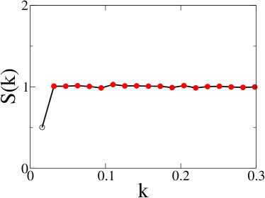
Figure 28: Structure factor for the 1D system with energy $E=S(q)\cdot(1/S_{0}-1)$, where $q$ is the smallest wave vector and $S_{0}=0.5$, at temperature $k_{B}T=1$. As discussed in the text, the effect of this energy is to constrain the structure factor at $q$ to $S_{0}=0.5$ (unfilled circle), and leave the structure factor at other wave vectors unconstrained (solid red circles).

We now move on to constraining the structure factor at multiple, non-independent wave vectors in order to realize the structure factor of the 1D “fermionic” system. Since the structure factor at multiple wave vectors are constrained, Eq. (40) is inexact due to correlations between structure-factor values at different wave vectors. To find out how inexact it is, we again performed molecular dynamics simulations. We define the energy

$$E=\sum_{|\mathbf{k}|<2\pi}{\tilde{v}}(\mathbf{k})\mathcal{S}(\mathbf{k}),$$ (94)

where ${\tilde{v}}(\mathbf{k})$ is given in (40). Here the summation beyond $|\mathbf{k}|=2\pi$ is unnecessary because for such $\mathbf{k}$ vectors, $S_{0}(\mathbf{k})=1$ and ${\tilde{v}}(\mathbf{k})$ vanishes. As previously discussed, we performed a molecular dynamics simulation with with $N=400$ particles at $k_{B}T=1$. The resulting structure factor, shown in Fig. 29, exhibits a noticeable deviation from its target $S_{0}(\mathbf{k})$.

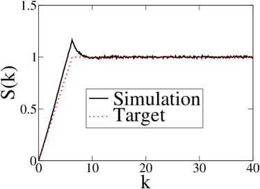
Figure 29: Structure factor for the 1D system with energy given in Eq. (94), in which $S_{0}(\mathbf{k})$ is given in Eq. (58), at temperature $k_{B}T=1$.

Since we were not able to derive an appropriate ${\tilde{v}}(\mathbf{k})$ for the general case of multiple non-independent $\mathbf{k}$ vectors, we could not meet these constraints by simply performing molecular dynamics simulations. We must therefore use the method presented in Sec. II.3 [minimizing $\Phi$ in Eq. (49) for $N_{c}=100$ configurations simultaneously].

One conclusion of our theoretical formalism is that our reconstructed configurations are drawn from the canonical ensemble of a pairwise additive interaction at some positive temperature. We can test this conclusion because the fermionic systems in one dimension also correspond to an equilibrium state of a logarithmic pairwise-additive potential with $\beta=2$. By Henderson’s theorem Henderson (1974), our targeted system and the fermionic system are both equilibrium states of the same pair potential, and thus the two systems should have the same higher-order statistics ($g_{3}$, $g_{4}$, $\cdots$). To check this conclusion, we computed the three-body correlation functions of our targeted system and compare with the analytical result of the fermionic system in Fig. 30. In general, $g_{3}$ is a function of three vectors: $\mathbf{r}_{12}$, $\mathbf{r}_{13}$, and $\mathbf{r}_{23}$. However, in 1D, we can set $\mathbf{r}_{12}=r_{1}$, $\mathbf{r}_{13}=r_{2}$, and $\mathbf{r}_{23}=r_{1}+r_{2}$, and then $g_{3}$ becomes a function of two scalars, $r_{1}$ and $r_{2}$. The difference between the numerically found $g_{3}(r_{1},r_{2})$ of the targeted system and the analytical $g_{3}(r_{1},r_{2})$ of the fermi-sphere system is two orders of magnitudes smaller than unity, and appears completely random with no systematic trend, consistent with our reasoning.

By contrast, the one-dimensional Lorentzian $S(k)$ target is also realized by a determinantal point process with an analytically known $g_{3}$ Costin and Lebowitz (2004), but it is not an equilibrium state of a pairwise additive potential Torquato et al. (2008). Therefore, the difference between the analytic $g_{3}$ for the determinantal point process and the numerical $g_{3}$ of the reconstructed system exhibits a peak much stronger than statistical noise at around $r_{1}=r_{2}=0.3$. The statistically significant difference is consistent with our theory that the reconstructed configurations are drawn from an equilibrium state of a pair potential, and therefore must be different from determinantal point processes not realizable by pair potentials. We have similarly verified that the exact analytical expression for $g_{3}$ of the 2D fermionic system differs from the numerically determined $g_{3}$ of the reconstructed system with the same pair statistics, which is expected since 2D fermionic systems also involve $n$-particle interactions with $n\geq 3$ Torquato et al. (2008).

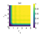
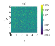
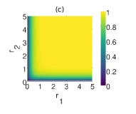
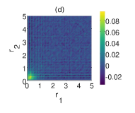
Figure 30: (a): Analytical three-body correlation function, $g_{3}(r_{1},r_{2})$, of the 1D fermi-sphere system. (b): The difference in $g_{3}$ between the targeted system and the 1D fermi-sphere system, $\Delta g_{3}(r_{1},r_{2})=g_{3}^{\mbox{fermionic}}(r_{1},r_{2})-g_{3}^{\mbox{targeted}}(r_{1},r_{2})$. (c) and (d): Same as (a) and (b), except for 1D Lorentzian target.

We now show numerical evidence that the structure factor at a constrained $\mathbf{k}$ vector is exponentially distributed. In Fig. 31, we plot the distribution of single-configuration structure factors at two different wave vectors for four different targets. After normalizing $S(\mathbf{k})$ by its mean, $S_{0}(\mathbf{k})$, all results collapse onto a single straight line in a semi-logarithmic plot, demonstrating that $S(\mathbf{k})$ is indeed exponentially distributed in all cases.

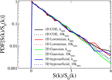
Figure 31: Probability density function (PDF) of the structure factor, normalized by the target, at two different wave vectors for four different targets. The two wave vectors are $k_{\mbox{min}}$, the minimum wave vector in the $x$ direction, and $10k_{\mbox{min}}$. The targets are 1D COE [Eq. (54)], 1D Lorentzian [Eq. (67)], 2D Gaussian [Eq. (71)], and 3D hyposurficial [Eq. (89)]. Since the structure factor is always exponentially distributed, the normalized plot for different cases falls on a single strait line on a plot on a semi-logarithmic scale.

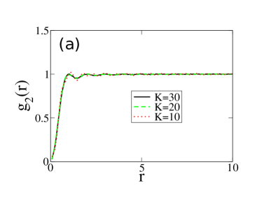
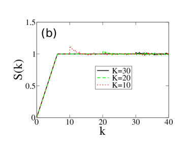
Figure 32: Pair correlation function and structure factor obtained by targeting Eq. (58) at various $K$’s.

Lastly, we explore the effect of changing the cutoff value $K$. The results are presented in Fig. 32. With $K=10$, the structure factor develops a discontinuity at the cutoff. However, as we increase $K$ to 30, the discontinuity diminishes. We have also explored many other targets, detailed in the rest of the paper, and always find that when $K$ is sufficiently large, the structure factor is continuous at the cutoff. In summary, except for some special cases discussed in the paper, the cutoff value of $K=30$ is generally suitable for one-dimensional targets that we examined, and $K=15$ is generally suitable for two- and three-dimensional targets reported here.

References

- Hansen and McDonald (2013) J. P. Hansen and I. R. McDonald, Theory of Simple Liquids, 4th ed. (Academic Press, New York, 2013).
- Torquato and Stillinger (2006a) S. Torquato and F. H. Stillinger, “New conjectural lower bounds on the optimal density of sphere packings,” Exp. Math. 15, 307–331 (2006a).
- Jiao et al. (2010) Y. Jiao, F. H. Stillinger, and S. Torquato, “Geometrical ambiguity of pair statistics: Point configurations,” Phys. Rev. E 81, 011105 (2010).
- Yamada (1961) M. Yamada, “Geometrical study of the pair distribution function in the many-body problem,” Prog. Theor. Phys. 25, 579–594 (1961).
- Lenard (1973) A. Lenard, “Correlation functions and the uniqueness of the state in classical statistical mechanics,” Commun. Math. Phys. 30, 35–44 (1973).
- Lenard (1975a) A. Lenard, “States of classical statistical mechanical systems of infinitely many particles I,” Arch. Rational Mech. Anal. 59, 219–239 (1975a).
- Lenard (1975b) A. Lenard, “States of classical statistical mechanical systems of infinitely many particles II. Characterization of correlation measures,” Arch. Rational Mech. Anal. 59, 241–256 (1975b).
- Rintoul (1997) S. Rintoul, M. D.and Torquato, “Reconstruction of the structure of dispersions,” J. Colloid Interface Sci. 186, 467–476 (1997).
- Crawford et al. (2003) J. Crawford, S. Torquato, and F. H. Stillinger, “Aspects of correlation function realizability,” J. Chem. Phys. 119, 7065–7074 (2003).
- Costin and Lebowitz (2004) O. Costin and J. L. Lebowitz, “On the construction of particle distributions with specified single and pair densities,” J. Phys. Chem. B 108, 19614–19618 (2004).
- Koralov (2005) L. Koralov, “Existence of pair potential corresponding to specified density and pair correlation,” Lett. Math. Phys. 71, 135–148 (2005).
- Stillinger and Torquato (2005) F. H. Stillinger and S. Torquato, “Realizability issues for iso-g (2) processes,” Mol. Phys. 103, 2943–2949 (2005).
- Uche et al. (2006a) O. U. Uche, F. H. Stillinger, and S. Torquato, “On the realizability of pair correlation functions,” Physica A 360, 21–36 (2006a).
- Kuna et al. (2007) T. Kuna, J. L. Lebowitz, and E. R. Speer, “Realizability of point processes,” J. Stat. Phys. 129, 417–439 (2007). These authors also report the interesting result that given a sufficiently low and a realizable , can be perturbed arbitrarily.
- Kuna et al. (2011) T. Kuna, J. L. Lebowitz, and E. R. Speer, “Necessary and sufficient conditions for realizability of point processes,” Ann. Appl. Probab. 21, 1253–1281 (2011).
- (16) R. Lachieze-Rey and I. Molchanov, “Regularity conditions in the realisability problem with applications to point processes and random closed sets,” Ann. Appl. Probab. 25, 116–149 (2015).
- Torquato and Stillinger (2003) S. Torquato and F. H. Stillinger, “Local density fluctuations, hyperuniformity, and order metrics,” Phys. Rev. E 68, 041113 (2003).
- Torquato (2018) S. Torquato, “Hyperuniform states of matter,” Physics Reports 745, 1–95 (2018).
- Chremos and Douglas (2017) A. Chremos and J. F. Douglas, “Particle localization and hyperuniformity of polymer-grafted nanoparticle materials,” Annalen der Physik 529, 1600342 (2017).
- Ghosh and Lebowitz (2018) S. Ghosh and J. L. Lebowitz, “Generalized stealthy hyperuniform processes: Maximal rigidity and the bounded holes conjecture,” Commun. Math. Phys. 363, 97–110 (2018).
- Brauchart et al. (2018) J. S. Brauchart, P. J. Grabner, W. B. Kusner, and J. Ziefle, “Hyperuniform point sets on the sphere: Probabilistic aspects,” arXiv preprint arXiv:1809.02645 (2018).
- Crowley et al. (2018) P. J. Crowley, C. R. Laumann, and S. Gopalakrishnan, “Quantum criticality in Ising chains with random hyperuniform couplings,” arXiv preprint arXiv:1809.04595 (2018).
- Lei et al. (2019) Q.-L. Lei, M. P. Ciamarra, and R. Ni, “Nonequilibrium strongly hyperuniform fluids of circle active particles with large local density fluctuations,” Sci. Adv. 5, eaau7423 (2019).
- Lacroix-A-Chez-Toine et al. (2019) B. Lacroix-A-Chez-Toine, J. A. M. Garzón, C. S. H. Calva, I. P. Castillo, A. Kundu, S. N. Majumdar, and G. Schehr, “Intermediate deviation regime for the full eigenvalue statistics in the complex Ginibre ensemble,” Phys. Rev. E 100, 012137 (2019).
- Florescu et al. (2009) M. Florescu, S. Torquato, and P. J. Steinhardt, “Designer disordered materials with large complete photonic band gaps,” Proc. Nat. Acad. Sci. 106, 20658–20663 (2009).
- Ricouvier et al. (2019) J. Ricouvier, P. Tabeling, and P. Yazhgur, “Foam as a self-assembling amorphous photonic band gap material,” Proc. Nat. Acad. Sci. 116, 9202–9207 (2019).
- Zito et al. (2015) G. Zito, G. Rusciano, G. Pesce, A. Dochshanov, and A. Sasso, “Surface-enhanced raman imaging of cell membrane by a highly homogeneous and isotropic silver nanostructure,” Nanoscale 7, 8593–8606 (2015).
- Leseur et al. (2016) O. Leseur, R. Pierrat, and R. Carminati, “High-density hyperuniform materials can be transparent,” Optica 3, 763–767 (2016).
- Ma et al. (2016) T. Ma, H. Guerboukha, M. Girard, A. D. Squires, R. A. Lewis, and M. Skorobogatiy, “3D printed hollow-core terahertz optical waveguides with hyperuniform disordered dielectric reflectors,” Adv. Opt. Mater. 4, 2085–2094 (2016).
- Saavedra et al. (2016) J. R. M. Saavedra, D. Castells-Graells, and F. J. G. de Abajo, “Smith-purcell radiation emission in aperiodic arrays,” Phys. Rev. B 94, 035418 (2016).
- Uche et al. (2006b) O. U. Uche, S. Torquato, and F. H. Stillinger, “Collective coordinate control of density distributions,” Phys. Rev. E 74, 031104 (2006b).
- Batten et al. (2008) R. D. Batten, F. H. Stillinger, and S. Torquato, “Classical disordered ground states: Super-ideal gases and stealth and equi-luminous materials,” J. Appl. Phys. 104, 033504–033504 (2008).
- Soshnikov (2000) A. Soshnikov, “Determinantal random point fields,” Russian Mathematical Surveys 55, 923–975 (2000).
- Mehta (2004) M. L. Mehta, Random matrices, Vol. 142 (Academic press, Cambridge, MA, USA, 2004).
- Torquato et al. (2008) S. Torquato, A. Scardicchio, and C. E. Zachary, “Point processes in arbitrary dimension from fermionic gases, random matrix theory, and number theory,” J. Stat. Mech. Theor. Exp. , P11019 (2008).
- Hough et al. (2009) J. B. Hough, M. Krishnapur, Y. Peres, and B. Virág, Zeros of Gaussian analytic functions and determinantal point processes, Vol. 51 (American Mathematical Society, Providence, RI, 2009).
- Abreu et al. (2017) L. D. Abreu, J. M. Pereira, J. L. Romero, and S. Torquato, “The Weyl-Heisenberg ensemble: Hyperuniformity and higher landau levels,” J. Stat. Mech.: Th. and Exper. 2017, 043103 (2017).
- (38) F. Martelli, S. Torquato, N. Giovambattista, and R. Car, “Large-Scale Structure and Hyperuniformity of Amorphous Ices,” Phys. Rev. Lett. 119, 136002 (2017).
- Zachary and Torquato (2011) C. E. Zachary and S. Torquato, “Anomalous local coordination, density fluctuations, and void statistics in disordered hyperuniform many-particle ground states,” Phys. Rev. E 83, 051133 (2011).
- Zhang et al. (2016) G. Zhang, F. H. Stillinger, and S. Torquato, “The perfect glass paradigm: Disordered hyperuniform glasses down to absolute zero,” Sci. Rep. 6 (2016).
- (41) T. R. Kirkpatrick, D. Thirumalai, and P. G. Wolynes, “Scaling concepts for the dynamics of viscous liquids near an ideal glassy state,” Phys. Rev. A 40, 1045 (1989).
- (42) G. Parisi, M. Picco, and N. Sourlas, “Scale invariance and self-averaging in disordered systems,” Europhys. Lett. 66, 4 (2004).
- Fan et al. (1991) Y. Fan, J. K Percus, D. K Stillinger, and F. H. Stillinger, “Constraints on collective density variables: One dimension,” Phys. Rev. A 44, 2394 (1991).
- Uche et al. (2004) O. U. Uche, F. H. Stillinger, and S. Torquato, “Constraints on collective density variables: Two dimensions,” Phys. Rev. E 70, 046122 (2004).
- Torquato et al. (2015) S. Torquato, G. Zhang, and F. H. Stillinger, “Ensemble theory for stealthy hyperuniform disordered ground states,” Phys. Rev. X 5, 021020 (2015).
- Nocedal (1980) J. Nocedal, “Updating quasi-newton matrices with limited storage,” Math. Comp. 35, 773–782 (1980).
- Liu and Nocedal (1989) D. C. Liu and J. Nocedal, “On the limited memory bfgs method for large scale optimization,” Math. Programming 45, 503–528 (1989).
- (48) S. G. Johnson, “The nlopt nonlinear-optimization package,” Http://ab-initio.mit.edu/nlopt.
- Scardicchio et al. (2009) A. Scardicchio, C. E. Zachary, and S. Torquato, “Statistical properties of determinantal point processes in high-dimensional Euclidean spaces,” Phys. Rev. E 79, 041108 (2009).
- Forrester (2016) P. J. Forrester, “Analogies between random matrix ensembles and the one-component plasma in two-dimensions,” Nucl. Phys. B 904, 253–281 (2016).
- Henderson (1974) R. L. Henderson, “A uniqueness theorem for fluid pair correlation functions,” Phys. Lett. A 49, 197–198 (1974).
- (52) Henderson claimed that a modification of his proof for positive temperature () can be used to prove the same uniqueness theorem for a system in its ground state (). However, this cannot be generally true for a classical statistical mechanical system at , since there are generally an infinite number of different pair potential functions consistent with a particular ground-state structure. Indeed, the existence of “universally optimal” solutions for certain ground-state structures, as described in Refs. Cohn and Kumar (2007) and Cohn et al. (2019), rigorously supports this conclusion.
- Cohn and Kumar (2007) H. Cohn and A. Kumar, “Universally optimal distribution of points on spheres,” J. Am. Math. Soc. 20, 99–148 (2007).
- Cohn et al. (2019) H. Cohn, A. Kumar, S. D. Miller, D. Radchenko, and M. Viazovska, “Universal optimality of the and leech lattices and interpolation formulas,” arXiv preprint arXiv:1902.05438 (2019).
- Jancovici (1981) B. Jancovici, “Exact results for the two-dimensional one-component plasma,” Phys. Rev. Lett. 46, 386 (1981).
- (56) G. Zhang, F. Stillinger, and S. Torquato, “Classical Many-Particle Systems with Unique Disordered Ground States,” Phys. Rev. E, 96, 042146 (2017).
- Andreanov et al. (2016) A. Andreanov, A. Scardicchio, and S. Torquato, “Extreme lattices: Symmetries and decorrelation,” J. Stat. Mech.: Th. & Exper. 2016, 113301 (2016).
- (58) F. H. Stillinger and S. Torquato, “Structural Degeneracy in Pair Distance Distributions,” J. Chem. Phys., 150, 204125 (2019).
- (59) S. Torquato, “Inverse Optimization Techniques for Targeted Self-Assembly,” Soft Matter 5, 1157 (2009).
- (60) G. Zhang, F. H. Stillinger, and S. Torquato, “Probing the Limitations of Isotropic Pair Potentials to Produce Ground-State Structural Extremes via Inverse Statistical Mechanics,” Phys. Rev. E, 88, 042309 (2013).
- (61) B. A. Lindquist, R. B. Jadrich, and T. M. Truskett, “Inverse design for self-assembly via on-the-fly optimization,” J. Chem. Phys. 145, 111101 (2016).
- (62) R. B. Jadrich, B. A. Lindquist, and T. M. Truskett, “Probabilistic inverse design for self-assembling materials,” J. Chem. Phys. 146, 184103 (2017).
- (63) M. C. Rechtsman and S. Torquato, “Effective Dielectric Tensor for Electromagnetic Wave Propagation in Random Media,” J. Appl. Phys., 103, 084901 (2008).
- (64) S. Torquato, Random Heterogeneous Materials: Microstructure and Macroscopic Properties. (Springer-Verlag, Berlin, 2002).