TaPas: Weakly Supervised Table Parsing via Pre-training

Abstract

Answering natural language questions over tables is usually seen as a semantic parsing task. To alleviate the collection cost of full logical forms, one popular approach focuses on weak supervision consisting of denotations instead of logical forms. However, training semantic parsers from weak supervision poses difficulties, and in addition, the generated logical forms are only used as an intermediate step prior to retrieving the denotation. In this paper, we present TaPas, an approach to question answering over tables without generating logical forms. TaPas trains from weak supervision, and predicts the denotation by selecting table cells and optionally applying a corresponding aggregation operator to such selection. TaPas extends BERT’s architecture to encode tables as input, initializes from an effective joint pre-training of text segments and tables crawled from Wikipedia, and is trained end-to-end. We experiment with three different semantic parsing datasets, and find that TaPas outperforms or rivals semantic parsing models by improving state-of-the-art accuracy on SQA from $55.1$ to $67.2$ and performing on par with the state-of-the-art on WikiSQL and WikiTQ, but with a simpler model architecture. We additionally find that transfer learning, which is trivial in our setting, from WikiSQL to WikiTQ, yields $48.7$ accuracy, $4.2$ points above the state-of-the-art.

1 Introduction

Question answering from semi-structured tables is usually seen as a semantic parsing task where the question is translated to a logical form that can be executed against the table to retrieve the correct denotation Pasupat and Liang (2015); Zhong et al. (2017); Dasigi et al. (2019); Agarwal et al. (2019). Semantic parsers rely on supervised training data that pairs natural language questions with logical forms, but such data is expensive to annotate.

In recent years, many attempts aim to reduce the burden of data collection for semantic parsing, including paraphrasing Wang et al. (2015), human in the loop Iyer et al. (2017); Lawrence and Riezler (2018) and training on examples from other domains Herzig and Berant (2017); Su and Yan (2017). One prominent data collection approach focuses on weak supervision where a training example consists of a question and its denotation instead of the full logical form Clarke et al. (2010); Liang et al. (2011); Artzi and Zettlemoyer (2013). Although appealing, training semantic parsers from this input is often difficult due to the abundance of spurious logical forms Berant et al. (2013); Guu et al. (2017) and reward sparsity Agarwal et al. (2019); Muhlgay et al. (2019).

In addition, semantic parsing applications only utilize the generated logical form as an intermediate step in retrieving the answer. Generating logical forms, however, introduces difficulties such as maintaining a logical formalism with sufficient expressivity, obeying decoding constraints (e.g. well-formedness), and the label bias problem Andor et al. (2016); Lafferty et al. (2001).

In this paper we present TaPas (for Table Parser), a weakly supervised question answering model that reasons over tables without generating logical forms. TaPas predicts a minimal program by selecting a subset of the table cells and a possible aggregation operation to be executed on top of them. Consequently, TaPas can learn operations from natural language, without the need to specify them in some formalism. This is implemented by extending BERT’s architecture Devlin et al. (2019) with additional embeddings that capture tabular structure, and with two classification layers for selecting cells and predicting a corresponding aggregation operator.

Importantly, we introduce a pre-training method for TaPas, crucial for its success on the end task. We extend BERT’s masked language model objective to structured data, and pre-train the model over millions of tables and related text segments crawled from Wikipedia. During pre-training, the model masks some tokens from the text segment and from the table itself, where the objective is to predict the original masked token based on the textual and tabular context.

Finally, we present an end-to-end differentiable training recipe that allows TaPas to train from weak supervision. For examples that only involve selecting a subset of the table cells, we directly train the model to select the gold subset. For examples that involve aggregation, the relevant cells and the aggregation operation are not known from the denotation. In this case, we calculate an expected soft scalar outcome over all aggregation operators given the current model, and train the model with a regression loss against the gold denotation.

In comparison to prior attempts to reason over tables without generating logical forms Neelakantan et al. (2015); Yin et al. (2016); Müller et al. (2019), TaPas achieves better accuracy, and holds several advantages: its architecture is simpler as it includes a single encoder with no auto-regressive decoding, it enjoys pre-training, tackles more question types such as those that involve aggregation, and directly handles a conversational setting.

We find that on three different semantic parsing datasets, TaPas performs better or on par in comparison to other semantic parsing and question answering models. On the conversational SQA Iyyer et al. (2017), TaPas improves state-of-the-art accuracy from $55.1$ to $67.2$, and achieves on par performance on WikiSQL Zhong et al. (2017) and WikiTQ Pasupat and Liang (2015). Transfer learning, which is simple in TaPas, from WikiSQL to WikiTQ achieves 48.7 accuracy, $4.2$ points higher than state-of-the-art. Our code and pre-trained model are publicly available at https://github.com/google-research/tapas.

2 TaPas Model

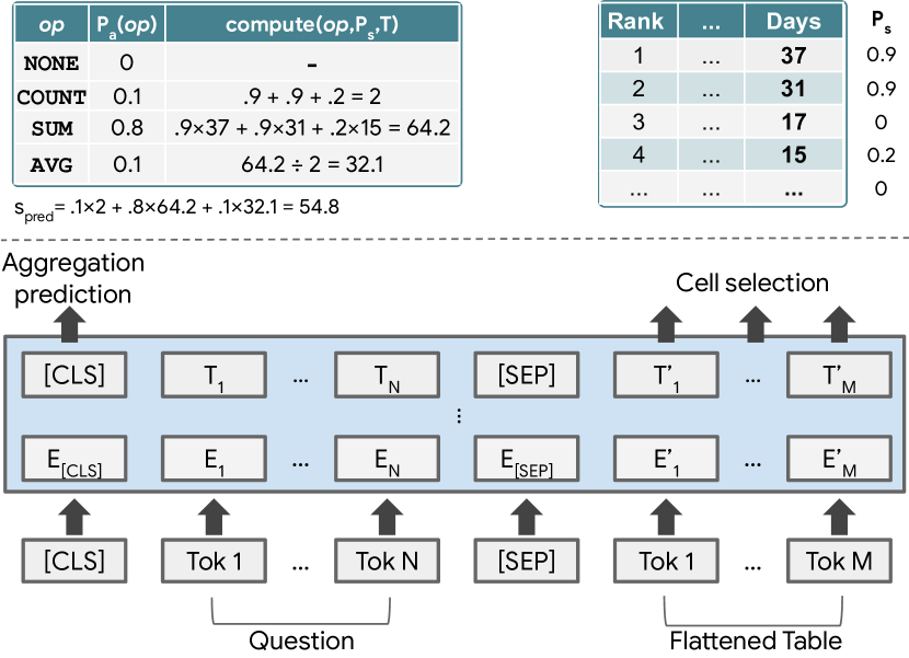
Figure 1: TaPas model (bottom) with example model outputs for the question: “Total number of days for the top two”. Cell prediction (top right) is given for the selected column’s table cells in bold (zero for others) along with aggregation prediction (top left).

Our model’s architecture (Figure 1) is based on BERT’s encoder with additional positional embeddings used to encode tabular structure (visualized in Figure 2). We flatten the table into a sequence of words, split words into word pieces (tokens) and concatenate the question tokens before the table tokens. We additionally add two classification layers for selecting table cells and aggregation operators that operate on the cells. We now describe these modifications and how inference is performed.

Additional embeddings

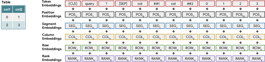
Figure 2: Encoding of the question “query?” and a simple table using the special embeddings of TaPas. The previous answer embeddings are omitted for brevity.

We add a separator token between the question and the table, but unlike Hwang et al. (2019) not between cells or rows. Instead, the token embeddings are combined with table-aware positional embeddings before feeding them to the model. We use different kinds of positional embeddings:

• Position ID is the index of the token in the flattened sequence (same as in BERT).

• Segment ID takes two possible values: 0 for the question, and 1 for the table header and cells.

• Column / Row ID is the index of the column/row that this token appears in, or 0 if the token is a part of the question.

• Rank ID if column values can be parsed as floats or dates, we sort them accordingly and assign an embedding based on their numeric rank (0 for not comparable, 1 for the smallest item, $i+1$ for an item with rank $i$). This can assist the model when processing questions that involve superlatives, as word pieces may not represent numbers informatively Wallace et al. (2019).

• Previous Answer given a conversational setup where the current question might refer to the previous question or its answers (e.g., question 5 in Figure 3), we add a special embedding that marks whether a cell token was the answer to the previous question (1 if the token’s cell was an answer, or 0 otherwise).

Cell selection

This classification layer selects a subset of the table cells. Depending on the selected aggregation operator, these cells can be the final answer or the input used to compute the final answer. Cells are modelled as independent Bernoulli variables. First, we compute the logit for a token using a linear layer on top of its last hidden vector. Cell logits are then computed as the average over logits of tokens in that cell. The output of the layer is the probability $p^{(c)}_{\text{s}}$ to select cell $c$. We additionally found it useful to add an inductive bias to select cells within a single column. We achieve this by introducing a categorical variable to select the correct column. The model computes the logit for a given column by applying a new linear layer to the average embedding for cells appearing in that column. We add an additional column logit that corresponds to selecting no column or cells. We treat this as an extra column with no cells. The output of the layer is the probability $p_{\mathrm{col}}^{(co)}$ to select column $co$ computed using softmax over the column logits. We set cell probabilities $p_{s}^{(c)}$ outside the selected column to $0$.

Aggregation operator prediction

Semantic parsing tasks require discrete reasoning over the table, such as summing numbers or counting cells. To handle these cases without producing logical forms, TaPas outputs a subset of the table cells together with an optional aggregation operator. The aggregation operator describes an operation to be applied to the selected cells, such as SUM, COUNT, AVERAGE or NONE. The operator is selected by a linear layer followed by a softmax on top of the final hidden vector of the first token (the special [CLS] token). We denote this layer as $p_{a}(op)$, where $op$ is some aggregation operator.

Inference

We predict the most likely aggregation operator together with a subset of the cells (using the cell selection layer). To predict a discrete cell selection we select all table cells for which their probability is larger than $0.5$. These predictions are then executed against the table to retrieve the answer, by applying the predicted aggregation over the selected cells.

3 Pre-training

Following the recent success of pre-training models on textual data for natural language understanding tasks, we wish to extend this procedure to structured data, as an initialization for our table parsing task. To this end, we pre-train TaPas on a large number of tables from Wikipedia. This allows the model to learn many interesting correlations between text and the table, and between the cells of a columns and their header.

We create pre-training inputs by extracting text-table pairs from Wikipedia. We extract 6.2M tables: 3.3M of class Infobox and 2.9M of class WikiTable. We consider tables with at most 500 cells. All of the end task datasets we experiment with only contain horizontal tables with a header row with column names. Therefore, we only extract Wiki tables of this form using the <th> tag to identify headers. We furthermore, transpose Infoboxes into a table with a single header and a single data row. The tables, created from Infoboxes, are arguably not very typical, but we found them to improve performance on the end tasks.

As a proxy for questions that appear in the end tasks, we extract the table caption, article title, article description, segment title and text of the segment the table occurs in as relevant text snippets. In this way we extract 21.3M snippets.

We convert the extracted text-table pairs to pre-training examples as follows: Following Devlin et al. (2019), we use a masked language model pre-training objective. We also experimented with adding a second objective of predicting whether the table belongs to the text or is a random table but did not find this to improve the performance on the end tasks. This is aligned with Liu et al. (2019) that similarly did not benefit from a next sentence prediction task.

For pre-training to be efficient, we restrict our word piece sequence length to a certain budget (e.g., we use 128 in our final experiments). That is, the combined length of tokenized text and table cells has to fit into this budget. To achieve this, we randomly select a snippet of $8$ to $16$ word pieces from the associated text. To fit the table, we start by only adding the first word of each column name and cell. We then keep adding words turn-wise until we reach the word piece budget. For every table we generate 10 different snippets in this way.

We follow the masking procedure introduced by BERT. We use whole word masking for the text, and we find it beneficial to apply whole cell masking (masking all the word pieces of the cell if any of its pieces is masked) to the table as well.

We note that we additionally experimented with data augmentation, which shares a similar goal to pre-training. We generated synthetic pairs of questions and denotations over real tables via a grammar, and augmented these to the end tasks training data. As this did not improve end task performance significantly, we omit these results.

4 Fine-tuning

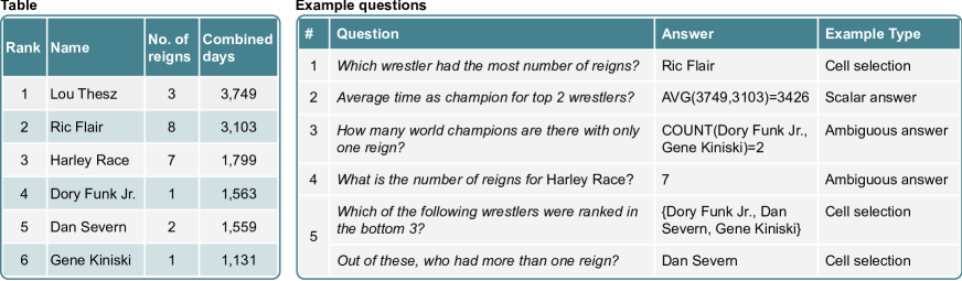
Figure 3: A table (left) with corresponding example questions (right). The last example is conversational.

Overview

We formally define table parsing in a weakly supervised setup as follows. Given a training set of $N$ examples $\{(x_{i},T_{i},y_{i})\}_{i=1}^{N}$, where $x_{i}$ is an utterance, $T_{i}$ is a table and $y_{i}$ is a corresponding set of denotations, our goal is to learn a model that maps a new utterance $x$ to a program $z$, such that when $z$ is executed against the corresponding table $T$, it yields the correct denotation $y$. The program $z$ comprises a subset of the table cells and an optional aggregation operator. The table $T$ maps a table cell to its value.

As a pre-processing step described in Section 5.1, we translate the set of denotations $y$ for each example to a tuple $(C,s)$ of cell coordinates $C$ and a scalar $s$, which is only populated when $y$ is a single scalar. We then guide training according to the content of $(C,s)$. For cell selection examples, for which $s$ is not populated, we train the model to select the cells in $C$. For scalar answer examples, where $s$ is populated but $C$ is empty, we train the model to predict an aggregation over the table cells that amounts to $s$. We now describe each of these cases in detail.

Cell selection

In this case $y$ is mapped to a subset of the table cell coordinates $C$ (e.g., question 1 in Figure 3). For this type of examples, we use a hierarchical model that first selects a single column and then cells from within that column only.

We directly train the model to select the column col which has the highest number of cells in $C$. For our datasets cells $C$ are contained in a single column and so this restriction on the model provides a useful inductive bias. If $C$ is empty we select the additional empty column corresponding to empty cell selection. The model is then trained to select cells $C\cap\textrm{col}$ and not select $(T\setminus C)\cap\textrm{col}$. The loss is composed of three components: (1) the average binary cross-entropy loss over column selections:

$$\mathcal{J}_{\text{columns}} =\frac{1}{\mathopen{|}\mathrm{Columns}\mathclose{|}}\sum_{\mathrm{co}\in\mathrm{Columns}}\mathrm{CE}(p_{\textrm{col}}^{(\textrm{co})},\mathbbm{1}_{\textrm{co}=\textrm{col}})$$

where the set of columns Columns includes the additional empty column, $\mathrm{CE}(\cdot)$ is the cross entropy loss, $\mathbbm{1}$ is the indicator function. (2) the average binary cross-entropy loss over column cell selections:

$$\mathcal{J}_{\text{cells}} =\frac{1}{\mathopen{|}\textrm{Cells}(\textrm{col})\mathclose{|}}\sum_{c\in\textrm{Cells}(\textrm{col})}\mathrm{CE}(p^{(c)}_{\text{s}},\mathbbm{1}_{c\in C}),$$

where $\textrm{Cells}(\textrm{col})$ is the set of cells in the chosen column. (3) As for cell selection examples no aggregation occurs, we define the aggregation supervision to be NONE (assigned to $op_{0}$), and the aggregation loss is:

$$\mathcal{J}_{\text{aggr}}=-\log p_{\text{a}}(op_{0}).$$

The total loss is then $\mathcal{J}_{\text{CS}}=\mathcal{J}_{\text{columns}}+\mathcal{J}_{\text{cells}}+\alpha\mathcal{J}_{\text{aggr}}$, where $\alpha$ is a scaling hyperparameter.

Scalar answer

In this case $y$ is a single scalar $s$ which does not appear in the table (i.e. $C=\emptyset$, e.g., question 2 in Figure 3). This usually corresponds to examples that involve an aggregation over one or more table cells. In this work we handle aggregation operators that correspond to SQL, namely COUNT, AVERAGE and SUM, however our model is not restricted to these.

For these examples, the table cells that should be selected and the aggregation operator type are not known, as these cannot be directly inferred from the scalar answer $s$. To train the model given this form of supervision one could search offline Dua et al. (2019); Andor et al. (2019) or online Berant et al. (2013); Liang et al. (2018) for programs (table cells and aggregation) that execute to $s$. In our table parsing setting, the number of spurious programs that execute to the gold scalar answer can grow quickly with the number of table cells (e.g., when $s=5$, each COUNT over any five cells is potentially correct). As with this approach learning can easily fail, we avoid it.

Instead, we make use of a training recipe where no search for correct programs is needed. Our approach results in an end-to-end differentiable training, similar in spirit to Neelakantan et al. (2015). We implement a fully differentiable layer that latently learns the weights for the aggregation prediction layer $p_{\text{a}}(\cdot)$, without explicit supervision for the aggregation type.

Specifically, we recognize that the result of executing each of the supported aggregation operators is a scalar. We then implement a soft differentiable estimation for each operator (Table 1), given the token selection probabilities and the table values: $\mbox{compute}(op,p_{\text{s}},T)$. Given the results for all aggregation operators we then calculate the expected result according to the current model:

$$s_{\text{pred}}=\sum_{i=1}\hat{p}_{\text{a}}(op_{i})\cdot\mbox{compute}(op_{i},p_{\text{s}},T),$$

where $\hat{p}_{\text{a}}(op_{i})=\frac{p_{\text{a}}(op_{i})}{\sum_{i=1}p_{\text{a}}(op_{i})}$ is a probability distribution normalized over aggregation operators excluding NONE.

$op$	$\mbox{compute}(op,p_{\text{s}},T)$
COUNT	$\sum_{c\in T}p^{(c)}_{\text{s}}$
SUM	$\sum_{c\in T}p^{(c)}_{\text{s}}\cdot T[c]$
AVERAGE	$\frac{\mbox{compute}(\texttt{SUM},p_{\text{s}},T)}{\mbox{compute}(\texttt{COUNT},p_{\text{s}},T)}$

Table 1: Aggregation operators soft implementation. AVERAGE approximation is discussed in Appendix D. Note that probabilities $p_{s}^{(c)}$ outside of the column selected by the model are set to 0.

We then calculate the scalar answer loss with Huber loss Huber (1964) given by:

$$\mathcal{J}_{\text{scalar}}=\begin{cases}0.5\cdot a^{2}&a\leq\delta\\ \delta\cdot a-0.5\cdot\delta^{2}&\text{otherwise}\end{cases}$$

where $a=\mathopen{|}s_{\text{pred}}-s\mathclose{|}$, and $\delta$ is a hyperparameter. Like Neelakantan et al. (2015), we find this loss is more stable than the squared loss. In addition, since a scalar answer implies some aggregation operation, we also define an aggregation loss that penalizes the model for assigning probability mass to the NONE class:

$$\mathcal{J}_{\text{aggr}}=-\log(\sum_{i=1}p_{\text{a}}(op_{i}))$$

The total loss is then $\mathcal{J}_{\text{SA}}=\mathcal{J}_{\text{aggr}}+\beta\mathcal{J}_{\text{scalar}}$, where $\beta$ is a scaling hyperparameter. As for some examples $\mathcal{J}_{\text{scalar}}$ can be very large, which leads to unstable model updates, we introduce a cutoff hyperparameter. Then, for a training example where $\mathcal{J}_{\text{scalar}}>\textit{cutoff}$, we set $\mathcal{J}=0$ to ignore the example entirely, as we noticed this behaviour correlates with outliers. In addition, as computation done during training is continuous, while that being done during inference is discrete, we further add a temperature that scales token logits such that $p_{\text{s}}$ would output values closer to binary ones.

Ambiguous answer

A scalar answer $s$ that also appears in the table (thus $C\neq\emptyset$) is ambiguous, as in some cases the question implies aggregation (question 3 in Figure 3), while in other cases a table cell should be predicted (question 4 in Figure 3). Thus, in this case we dynamically let the model choose the supervision (cell selection or scalar answer) according to its current policy. Concretely, we set the supervision to be of cell selection if $p_{\text{a}}(op_{0})\geq S$, where $0<S<1$ is a threshold hyperparameter, and the scalar answer supervision otherwise. This follows hard EM Min et al. (2019), as for spurious programs we pick the most probable one according to the current model.

5 Experiments

5.1 Datasets

We experiment with the following semantic parsing datasets that reason over single tables (see Table 2).

	WikiSQL	WikiTQ	SQA
Logical Form	✓	✗	✗
Conversational	✗	✗	✓
Aggregation	✓	✓	✗
Examples	80654	22033	17553
Tables	24241	2108	982

Table 2: Dataset statistics.

WikiTQ Pasupat and Liang (2015)

This dataset consists of complex questions on Wikipedia tables. Crowd workers were asked, given a table, to compose a series of complex questions that include comparisons, superlatives, aggregation or arithmetic operation. The questions were then verified by other crowd workers.

SQA Iyyer et al. (2017)

This dataset was constructed by asking crowd workers to decompose a subset of highly compositional questions from WikiTQ, where each resulting decomposed question can be answered by one or more table cells. The final set consists of $6,066$ question sequences ($2.9$ question per sequence on average).

WikiSQL Zhong et al. (2017)

This dataset focuses on translating text to SQL. It was constructed by asking crowd workers to paraphrase a template-based question in natural language. Two other crowd workers were asked to verify the quality of the proposed paraphrases.

As our model predicts cell selection or scalar answers, we convert the denotations for each dataset to $\langle$question, cell coordinates, scalar answer$\rangle$ triples. SQA already provides this information (gold cells for each question). For WikiSQL and WikiTQ, we only use the denotations. Therefore, we derive cell coordinates by matching the denotations against the table contents. We fill scalar answer information if the denotation contains a single element that can be interpreted as a float, otherwise we set its value to NaN. We drop examples if there is no scalar answer and the denotation can not be found in the table, or if some denotation matches multiple cells.

5.2 Experimental Setup

We apply the standard BERT tokenizer on questions, table cells and headers, using the same vocabulary of 32k word pieces. Numbers and dates are parsed in a similar way as in the Neural Programmer Neelakantan et al. (2017).

The official evaluation script of WikiTQ and SQA is used to report the denotation accuracy for these datasets. For WikiSQL, we generate the reference answer, aggregation operator and cell coordinates from the reference SQL provided using our own SQL implementation running on the JSON tables. However, we find that the answer produced by the official WikiSQL evaluation script is incorrect for approx. $2\%$ of the examples. Throughout this paper we report accuracies against our reference answers, but we explain the differences and also provide accuracies compared to the official reference answers in Appendix A.

We start pre-training from BERT-Large (see Appendix B for hyper-parameters). We find it beneficial to start the pre-training from a pre-trained standard text BERT model (while randomly initializing our additional embeddings), as this enhances convergence on the held-out set.

We run both pre-training and fine-tuning on a setup of 32 Cloud TPU v3 cores with maximum sequence length 512. In this setup pre-training takes around 3 days and fine-tuning around 10 hours for WikiSQL and WikiTQ and 20 hours for SQA (with the batch sizes from table 12). The resource requirements of our model are essentially the same as BERT-large.

For fine-tuning, we choose hyper-parameters using a black box Bayesian optimizer similar to Google Vizier Golovin et al. (2017) for WikiSQL and WikiTQ. For SQA we use grid-search. We discuss the details in Appendix B.

5.3 Results

All results report the denotation accuracy for models trained from weak supervision. We follow Niven and Kao (2019) and report the median for 5 independent runs, as BERT-based models can degenerate. We present our results for WikiSQL and WikiTQ in Tables 5 and 4 respectively. Table 5 shows that TaPas, trained in the weakly supervised setting, achieves close to state-of-the-art performance for WikiSQL ($83.6$ vs $83.9$ Min et al. (2019)). If given the gold aggregation operators and selected cell as supervision (extracted from the reference SQL), which accounts as full supervision to TaPas, the model achieves $86.4$. Unlike the full SQL queries, this supervision can be annotated by non-experts.

For WikiTQ the model trained only from the original training data reaches $42.6$ which surpass similar approaches Neelakantan et al. (2015). When we pre-train the model on WikiSQL or SQA (which is straight-forward in our setup, as we do not rely on a logical formalism), TaPas achieves $48.7$ and $48.8$, respectively.

Model	Dev	Test
Liang et al. (2018)	71.8	72.4
Agarwal et al. (2019)	74.9	74.8
Wang et al. (2019)	79.4	79.3
Min et al. (2019)	84.4	83.9
TaPas	85.1	83.6
TaPas (fully-supervised)	88.0	86.4

Table 3: WikiSQL denotation accuracy.

Model	Test
Pasupat and Liang (2015)	37.1
Neelakantan et al. (2017)	34.2
Haug et al. (2018)	34.8
Zhang et al. (2017)	43.7
Liang et al. (2018)	43.1
Dasigi et al. (2019)	43.9
Agarwal et al. (2019)	44.1
Wang et al. (2019)	44.5
TaPas	42.6
TaPas (pre-trained on WikiSQL)	48.7
TaPas (pre-trained on SQA)	48.8

Table 4: WikiTQ denotation accuracy.

For SQA, Table 5 shows that TaPas leads to substantial improvements on all metrics: Improving all metrics by at least $11$ points, sequence accuracy from $28.1$ to $40.4$ and average question accuracy from $55.1$ to $67.2$.

Model	ALL	SEQ	Q1	Q2	Q3
Pasupat and Liang (2015)	33.2	7.7	51.4	22.2	22.3
Neelakantan et al. (2017)	40.2	11.8	60.0	35.9	25.5
Iyyer et al. (2017)	44.7	12.8	70.4	41.1	23.6
Sun et al. (2018)	45.6	13.2	70.3	42.6	24.8
Müller et al. (2019)	55.1	28.1	67.2	52.7	46.8
TaPas	67.2	40.4	78.2	66.0	59.7

Table 5: SQA test results. ALL is the average question accuracy, SEQ the sequence accuracy, and QX, the accuracy of the X’th question in a sequence.

	SQA (SEQ)		WikiSQL		WikiTQ
all	39.0		84.7		29.0
-pos	36.7	-2.3	82.9	-1.8	25.3	-3.7
-ranks	34.4	-4.6	84.1	-0.6	30.7	+1.8
-{cols,rows}	19.6	-19.4	74.1	-10.6	17.3	-11.6
-table pre-training	26.5	-12.5	80.8	-3.9	17.9	-11.1
-aggregation	-		82.6	-2.1	23.1	-5.9

Table 6: Dev accuracy with different embeddings removed from the full model: positional (pos), numeric ranks (ranks), column (cols) and row (rows). The model without table pre-training was initialized from the original BERT model pre-trained on text only. The model without aggregation is only trained with the cell selection loss.

Model ablations

Table 6 shows an ablation study on our different embeddings. To this end we pre-train and fine-tune models with different features. As pre-training is expensive we limit it to $200,000$ steps. For all datasets we see that pre-training on tables and column and row embeddings are the most important. Positional and rank embeddings are also improving the quality but to a lesser extent.

We additionally find that when removing the scalar answer and aggregation losses (i.e., setting $\mathcal{J}_{\text{SA}=0}$) from TaPas, accuracy drops for both datasets. For WikiTQ, we observe a substantial drop in performance from $29.0$ to $23.1$ when removing aggregation. For WikiSQL performance drops from $84.7$ to $82.6$. The relatively small decrease for WikiSQL can be explained by the fact that most examples do not need aggregation to be answered. In principle, $17\%$ of the examples of the dev set have an aggregation (SUM, AVERAGE or COUNT), however, for all types we find that for more than $98\%$ of the examples the aggregation is only applied to one or no cells. In the case of SUM and AVERAGE, this means that most examples can be answered by selecting one or no cells from the table. For COUNT the model without aggregation operators achieves $28.2$ accuracy (by selecting $0$ or $1$ from the table) vs. $66.5$ for the model with aggregation. Note that $0$ and $1$ are often found in a special index column. These properties of WikiSQL make it challenging for the model to decide whether to apply aggregation or not. For WikiTQ on the other hand, we observe a substantial drop in performance from $29.0$ to $23.1$ when removing aggregation.

Qualitative Analysis on WikiTQ

We manually analyze $200$ dev set predictions made by TaPas on WikiTQ. For correct predictions via an aggregation, we inspect the selected cells to see if they match the ground truth. We find that $96\%$ of the correct aggregation predictions where also correct in terms of the cells selected. We further find that $14\%$ of the correct aggregation predictions had only one cell, and could potentially be achieved by cell selection, with no aggregation.

We also perform an error analysis and identify the following exclusive salient phenomena: (i) $12\%$are ambiguous (“Name at least two labels that released the group’s albums.”), have wrong labels or missing information ; (ii) $10\%$of the cases require complex temporal comparisons which could also not be parsed with a rich formalism such as SQL (“what country had the most cities founded in the 1830’s?”) ; (iii) in $16\%$ of the cases the gold denotation has a textual value that does not appear in the table, thus it could not be predicted without performing string operations over cell values ; (iv) on $10\%$, the table is too big to fit in $512$ tokens ; (v) on $13\%$ of the cases TaPas selected no cells, which suggests introducing penalties for this behaviour ; (vi) on $2\%$ of the cases, the answer is the difference between scalars, so it is outside of the model capabilities (“how long did anne churchill/spencer live?”) ; (vii) the other $37\%$ of the cases could not be classified to a particular phenomenon.

Pre-training Analysis

In order to understand what TaPas learns during pre-training we analyze its performance on 10,000 held-out examples. We split the data such that the tables in the held-out data do not occur in the training data.

	all	text	header	cell
all	71.4	68.8	96.6	63.4
word	74.1	69.7	96.9	66.6
number	53.9	51.7	83.6	53.2

Table 7: Mask LM accuracy on held-out data, when the target word piece is located in the text, table header, cell or anywhere (all) and the target is anything, a word or number.

Table 7 shows the accuracy of masked word pieces of different types and in different locations. We find that average accuracy across position is relatively high (71.4). Predicting tokens in the header of the table is easiest (96.6), probably because many Wikipedia articles use instances of the same kind of table. Predicting word pieces in cells is a bit harder (63.4) than predicting pieces in the text (68.8). The biggest differences can be observed when comparing predicting words (74.1) and numbers (53.9). This is expected since numbers are very specific and often hard to generalize. The soft-accuracy metric and example (Appendix C) demonstrate, however, that the model is relatively good at predicting numbers that are at least close to the target.

Limitations

TaPas handles single tables as context, which are able to fit in memory. Thus, our model would fail to capture very large tables, or databases that contain multiple tables. In this case, the table(s) could be compressed or filtered, such that only relevant content would be encoded, which we leave for future work.

In addition, although TaPas can parse compositional structures (e.g., question 2 in Figure 3), its expressivity is limited to a form of an aggregation over a subset of table cells. Thus, structures with multiple aggregations such as “number of actors with an average rating higher than 4” could not be handled correctly. Despite this limitation, TaPas succeeds in parsing three different datasets, and we did not encounter this kind of errors in Section 5.3. This suggests that the majority of examples in semantic parsing datasets are limited in their compositionality.

6 Related Work

Semantic parsing models are mostly trained to produce gold logical forms using an encoder-decoder approach Jia and Liang (2016); Dong and Lapata (2016). To reduce the burden in collecting full logical forms, models are typically trained from weak supervision in the form of denotations. These are used to guide the search for correct logical forms Clarke et al. (2010); Liang et al. (2011).

Other works suggested end-to-end differentiable models that train from weak supervision, but do not explicitly generate logical forms. Neelakantan et al. (2015) proposed a complex model that sequentially predicts symbolic operations over table segments that are all explicitly predefined by the authors, while Yin et al. (2016) proposed a similar model where the operations themselves are learned during training. Müller et al. (2019) proposed a model that selects table cells, where the table and question are represented as a Graph Neural Network, however their model can not predict aggregations over table cells. Cho et al. (2018) proposed a supervised model that predicts the relevant rows, column and aggregation operation sequentially. In our work, we propose a model that follow this line of work, with a simpler architecture than past models (as the model is a single encoder that performs computation for many operations implicitly) and more coverage (as we support aggregation operators over selected cells).

Finally, pre-training methods have been designed with different training objectives, including language modeling Dai and Le (2015); Peters et al. (2018); Radford et al. (2018) and masked language modeling Devlin et al. (2019); Lample and Conneau (2019). These methods dramatically boost the performance of natural language understanding models (Peters et al., 2018, inter alia). Recently, several works extended BERT for visual question answering, by pre-training over text-image pairs while masking different regions in the image Tan and Bansal (2019); Lu et al. (2019). As for tables, Chen et al. (2019) experimented with rendering a table into natural language so that it can be handled with a pre-trained BERT model. In our work we extend masked language modeling for table representations, by masking table cells or text segments.

7 Conclusion

In this paper we presented TaPas, a model for question answering over tables that avoids generating logical forms. We showed that TaPas effectively pre-trains over large scale data of text-table pairs and successfully restores masked words and table cells. We additionally showed that the model can fine-tune on semantic parsing datasets, only using weak supervision, with an end-to-end differentiable recipe. Results show that TaPas achieves better or competitive results in comparison to state-of-the-art semantic parsers.

In future work we aim to extend the model to represent a database with multiple tables as context, and to effectively handle large tables.

8 Acknowledgments

We would like to thank Yasemin Altun, Srini Narayanan, Slav Petrov, William Cohen, Massimo Nicosia, Syrine Krichene, Jordan Boyd-Graber and the anonymous reviewers for their constructive feedback, useful comments and suggestions. This work was completed in partial fulfillment for the PhD degree of the first author, which was also supported by a Google PhD fellowship.

Appendix A WikiSQL Execution Errors

col0	col1	col2	col3	col4	col5
Home team	Home team score	Away team	Away team score	Venue	Crowd
geelong	18.17 (125)	hawthorn	6.7 (43)	corio oval	9,000
footscray	8.18 (66)	south melbourne	11.18 (84)	western oval	12,500
fitzroy	11.5 (71)	richmond	8.12 (60)	brunswick street oval	14,000
north melbourne	6.12 (48)	essendon	14.11 (95)	arden street oval	8,000
st kilda	14.7 (91)	collingwood	17.13 (115)	junction oval	16,000
melbourne	12.11 (83)	carlton	11.11 (77)	mcg	31,481

Question	What was the away team’s score when the crowd at Arden Street Oval was larger than 31,481?
SQL Query	SELECT col3 AS result FROM table_2_10767641_15
	WHERE col5 > 31481.0 AND col4 = "arden street oval"
WikiSQL answer	["14.11 (95)"]
Our answer	[]
Question	What was the sum of the crowds at Western Oval?
SQL Query	SELECT SUM(col5) AS result FROM table_2_10767641_15
	WHERE col4 = "western oval"
WikiSQL answer	[12.0]
Our answer	[12500.0]

Table 8: Table “2-10767641-15” from WikiSQL. “col6” was removed. The “Crowd” column is of type “REAL” but the cell values are actually stored as “TEXT”. Below we have two questions from the training set with the answer that is produced by the WikiSQL evaluation script and the answer we derive.

In some tables, WikiSQL contains “REAL” numbers stored in “TEXT” format. This leads to incorrect results for some of the comparison and aggregation examples. These errors in the WikiSQL execution accuracy penalize systems that do their own execution (rather then producing an SQL query). Table 8 shows two examples where our result derivation and the one used by WikiSQL differ because the numbers in the “Crowd” (col5) column are not represented as numbers in the respective SQL table. Table 9 and 10 contain accuracies compared against the official and our answers.

Model	WikiSQL	TaPas
TaPas (no answer loss)	81.2	82.5
TaPas	83.9	85.1
TaPas (supervised)	86.6	88.0

Table 9: WikiSQL development denotation accuracy.

Model	WikiSQL	TaPas
TaPas (no answer loss)	80.1	81.2
TaPas	82.4	83.6
TaPas (supervised)	85.2	86.4

Table 10: WikiSQL test denotation accuracy.

Appendix B Hyperparameters

Parameter	Values	Scale
Learning rate	(1e-5, 3e-3)	Log
Warmup ratio	(0.0, 0.2)	Linear
Temperature	(0.1, 1)	Linear
Answer loss cutoff	(0.1, 10,000)	Log
Huber loss delta	(0.1, 10,000)	Log
Cell selection preference	(0, 1)	Linear
Reset cell selection weights	[0, 1]	Discrete

Table 11: Hyper-parameters for WikiSQL and WikiTQ. Values are constrained to either a range $(a,b)$ or a list $[a,b,c,\ldots]$.

Parameter	PRETRAIN	SQA	WikiSQL	WikiTQ
Training Steps	1,000,000	200,000	50,000	50,000
Learning rate	5e-5	1.25e-5	6.17164e-5	1.93581e-5
Warmup ratio	0.01	0.2	0.142400	0.128960
Temperature		1.0	0.107515	0.0352513
Answer loss cutoff			0.185567	0.664694
Huber loss delta			1265.74	0.121194
Cell selection preference			0.611754	0.207951
Batch size	512	128	512	512
Gradient clipping			10	10
Select one column		1	0	1
Reset cell selection weights		0	0	1

Table 12: Optimal hyper-parameters found for pretraining (PRETRAIN), SQA, WikiSQL and WikiTQ.

Appendix C Pre-training Example

In order to better understand how well the model predicts numbers, we relax our accuracy measure to a soft form of accuracy:

$$acc(x,y)=\begin{cases}1&\mbox{if }x=y\\ 0&\mbox{if $x$ or $y$ is not a number}\\ 1.0-\frac{|x-y|}{\max(x,y)}&\mbox{else}\end{cases}$$

With this soft metric we get an overall accuracy of 74.5 (instead of 71.4) and an accuracy of 80.5 (instead of 53.9) for numbers. Showing that the model is pretty good at guessing numbers that are at least close to the target. The following example demonstrates this:

Team	Pld	W	D	L	PF	PA	PD	Pts
South Korea	2	1	1	0	33	22	11	5
Spain	2	1	$\langle$1$\rangle$	$\langle$0$\rangle$	31	24	7	5
Zimbabwe	2	0	0	2	22	$\langle$43,40$\rangle$	- $\langle$19,18$\rangle$	2

Table 13: Table example from the Wikipedia page describing the 1997 Rugby World Cup Sevens. $\langle$x$\rangle$ marks a correct prediction and $\langle$x,y$\rangle$ an incorrect prediction.

In the example, the model correctly restores the Draw (D) and Loss (L) numbers for Spain. It fails to restore the Points For (PF) and Points Against (PA) for Zimbabwe, but gives close estimates. Note that the model also does not produce completely consistent results for each row we should have $\operatorname{PA}+\operatorname{PD}=\operatorname{PF}$ and the column sums of PF and PA should equal.

Appendix D The average of stochastic sets

Our approach to estimate aggregates of cells in the table operates directly on latent conditionally independent Bernoulli variables $G_{c}\sim\text{Bern}(p_{c})$ that indicate whether each cell is included in the aggregation and a latent categorical variable that indicates the chosen aggregation operation op: AVERAGE, SUM or COUNT. Given $G_{c}$ and the table values $T$ we can define a random subset $S\subseteq T$ where $p_{c}=P(c\in S)$ for each cell $c\in T$.

The expected value of $\texttt{COUNT}(S)=\sum_{c}G_{c}$ can be computed as $\sum_{c}p_{c}$ and $\texttt{SUM}(S)=\sum_{c}G_{c}T_{c}$ as $\sum_{c}p_{c}T_{c}$ as described in Table 1. For the average however, this is not straight-forward. We will see in what follows that the quotient of the expected sum and the count, which equals the weighed average of $T$ by $p_{c}$ in general is not the true expected value, which can be written as:

$$\mathbb{E}\left[\frac{\sum G_{c}T_{c}}{\sum G_{c}}\right]$$

This quantity differs from the weighted average, a key difference being that the weighted average is not sensitive to constants scaling all the output probabilities, which could in theory find optima where all the $p_{c}$ are below $0.5$ for example. By the linearity of the expectation we can write:

$$\sum_{c}T_{c}\mathbb{E}\left[\frac{G_{c}}{\sum_{j}G_{j}}\right]=\sum_{c}T_{c}p_{c}\mathbb{E}\left[\frac{1}{1+\sum_{j\neq c}G_{j}}\right]$$

So it comes down to computing that quantity $Q_{c}=\mathbb{E}\left[\frac{1}{X_{c}}\right]=\mathbb{E}\left[\frac{1}{1+\sum_{j\neq c}G_{j}}\right]$. The key observation is that this is the expectation of a reciprocal of a Poisson Binomial Distribution (a sum of Bernoulli variables) in the special case where one of the probabilities is $1$.

By using the Jensen inequality we get a lower bound on $Q_{c}$ as $\frac{1}{\mathbb{E}\left[X_{c}\right]}=\frac{1}{1+\sum_{j\neq c}p_{j}}$. Note that if instead we used $\frac{1}{\sum_{j}p_{j}}$ then we recover the weighted average, which is strictly bigger than the lower bound and in general not an upper or lower bound. We can get better approximations by computing the Taylor expansion using the moments of $X_{c}$ of order $k$:

$$Q_{c}=\mathbb{E}\left[\frac{1}{X_{c}}\right]\simeq \frac{1}{\mathbb{E}\left[X_{c}\right]}+\frac{\text{var}\left[X_{c}\right]}{\mathbb{E}\left[X_{c}\right]^{3}}+\cdots+$$

$$(-1)^{k}\frac{\mathbb{E}\left[\left(X_{c}-\mathbb{E}\left[X_{c}\right]\right)^{k}\right]}{\mathbb{E}\left[X_{c}\right]^{k+1}}$$

where $\text{var}\left[X_{c}\right]=\sum_{j\neq c}p_{j}(1-p_{j})$.

The full form for the zero and second order Taylor approximations are:

$$\texttt{AVERAGE}_{0}(T,p) =\sum_{c}T_{c}\frac{p_{c}}{1+\sum_{j\neq c}p_{j}}$$

$$\texttt{AVERAGE}_{2}(T,p) =\sum_{c}T_{c}\frac{p_{c}(1+\epsilon_{c})}{1+\sum_{j\neq c}p_{j}}$$

$$\text{with}\>\epsilon_{c} =\frac{\sum_{j\neq c}p_{j}(1-p_{j})}{(1+\sum_{j\neq c}p_{j})^{2}}$$

The approximations are then easy to write in any tensor computation language and will be differentiable. In this work we experimented with the zero and second order approximations and found small improvements over the weighted average baseline. It’s worth noting that in the dataset the proportion of average examples is very low. We expect this method to be more relevant in the more general setting.

References

- Agarwal et al. (2019) R. Agarwal, C. Liang, D. Schuurmans, and M. Norouzi. 2019. Learning to generalize from sparse and underspecified rewards. arXiv preprint arXiv:1902.07198.
- Andor et al. (2016) D. Andor, C. Alberti, D. Weiss, A. Severyn, A. Presta, K. Ganchev, S. Petrov, and M. Collins. 2016. Globally normalized transition-based neural networks. arXiv preprint arXiv:1603.06042.
- Andor et al. (2019) Daniel Andor, Luheng He, Kenton Lee, and Emily Pitler. 2019. Giving bert a calculator: Finding operations and arguments with reading comprehension. arXiv preprint arXiv:1909.00109.
- Artzi and Zettlemoyer (2013) Y. Artzi and L. Zettlemoyer. 2013. Weakly supervised learning of semantic parsers for mapping instructions to actions. Transactions of the Association for Computational Linguistics (TACL), 1:49–62.
- Berant et al. (2013) J. Berant, A. Chou, R. Frostig, and P. Liang. 2013. Semantic parsing on Freebase from question-answer pairs. In Empirical Methods in Natural Language Processing (EMNLP).
- Chen et al. (2019) Wenhu Chen, Hongmin Wang, Jianshu Chen, Yunkai Zhang, Hong Wang, Shiyang Li, Xiyou Zhou, and William Yang Wang. 2019. Tabfact: A large-scale dataset for table-based fact verification. ArXiv, abs/1909.02164.
- Cho et al. (2018) Minseok Cho, Reinald Kim Amplayo, Seung won Hwang, and Jonghyuck Park. 2018. Adversarial tableqa: Attention supervision for question answering on tables. In ACML.
- Clarke et al. (2010) J. Clarke, D. Goldwasser, M. Chang, and D. Roth. 2010. Driving semantic parsing from the world’s response. In Computational Natural Language Learning (CoNLL), pages 18–27.
- Dai and Le (2015) A. M. Dai and Q. V. Le. 2015. Semi-supervised sequence learning. In Advances in Neural Information Processing Systems (NeurIPS).
- Dasigi et al. (2019) Pradeep Dasigi, Matt Gardner, Shikhar Murty, Luke Zettlemoyer, and Eduard Hovy. 2019. Iterative search for weakly supervised semantic parsing. In Proceedings of the 2019 Conference of the North American Chapter of the Association for Computational Linguistics: Human Language Technologies, Volume 1 (Long and Short Papers), pages 2669–2680.
- Devlin et al. (2019) Jacob Devlin, Ming-Wei Chang, Kenton Lee, and Kristina Toutanova. 2019. BERT: Pre-training of deep bidirectional transformers for language understanding. In Proceedings of the 2019 Conference of the North American Chapter of the Association for Computational Linguistics: Human Language Technologies, Volume 1 (Long and Short Papers), pages 4171–4186, Minneapolis, Minnesota. Association for Computational Linguistics.
- Dong and Lapata (2016) L. Dong and M. Lapata. 2016. Language to logical form with neural attention. In Association for Computational Linguistics (ACL).
- Dua et al. (2019) D. Dua, Y. Wang, P. Dasigi, G. Stanovsky, S. Singh, and M. Gardner. 2019. DROP: A reading comprehension benchmark requiring discrete reasoning over paragraphs. In North American Association for Computational Linguistics (NAACL).
- Golovin et al. (2017) Daniel Golovin, Benjamin Solnik, Subhodeep Moitra, Greg Kochanski, John Elliot Karro, and D. Sculley, editors. 2017. Google Vizier: A Service for Black-Box Optimization.
- Guu et al. (2017) K. Guu, P. Pasupat, E. Z. Liu, and P. Liang. 2017. From language to programs: Bridging reinforcement learning and maximum marginal likelihood. In Association for Computational Linguistics (ACL).
- Haug et al. (2018) T. Haug, O. Ganea, and P. Grnarova. 2018. Neural multi-step reasoning for question answering on semi-structured tables. In European Conference on Information Retrieval.
- Herzig and Berant (2017) J. Herzig and J. Berant. 2017. Neural semantic parsing over multiple knowledge-bases. In Association for Computational Linguistics (ACL).
- Huber (1964) P. J. Huber. 1964. Robust estimation of a location parameter. The Annals of Mathematical Statistics, 35(1):73–101.
- Hwang et al. (2019) Wonseok Hwang, Jinyeung Yim, Seunghyun Park, and Minjoon Seo. 2019. A comprehensive exploration on wikisql with table-aware word contextualization. arXiv preprint arXiv:1902.01069.
- Iyer et al. (2017) S. Iyer, I. Konstas, A. Cheung, J. Krishnamurthy, and L. Zettlemoyer. 2017. Learning a neural semantic parser from user feedback. In Association for Computational Linguistics (ACL).
- Iyyer et al. (2017) M. Iyyer, W. Yih, and M. Chang. 2017. Search-based neural structured learning for sequential question answering. In Association for Computational Linguistics (ACL).
- Jia and Liang (2016) R. Jia and P. Liang. 2016. Data recombination for neural semantic parsing. In Association for Computational Linguistics (ACL).
- Lafferty et al. (2001) J. Lafferty, A. McCallum, and F. Pereira. 2001. Conditional random fields: Probabilistic models for segmenting and labeling data. In International Conference on Machine Learning (ICML), pages 282–289.
- Lample and Conneau (2019) Guillaume Lample and Alexis Conneau. 2019. Cross-lingual language model pretraining. arXiv preprint arXiv:1901.07291.
- Lawrence and Riezler (2018) Carolin Lawrence and Stefan Riezler. 2018. Improving a neural semantic parser by counterfactual learning from human bandit feedback. In Proceedings of the 56th Annual Meeting of the Association for Computational Linguistics (Volume 1: Long Papers), pages 1820–1830, Melbourne, Australia. Association for Computational Linguistics.
- Liang et al. (2018) C. Liang, M. Norouzi, J. Berant, Q. Le, and N. Lao. 2018. Memory augmented policy optimization for program synthesis with generalization. In Advances in Neural Information Processing Systems (NeurIPS).
- Liang et al. (2011) P. Liang, M. I. Jordan, and D. Klein. 2011. Learning dependency-based compositional semantics. In Association for Computational Linguistics (ACL), pages 590–599.
- Liu et al. (2019) Yinhan Liu, Myle Ott, Naman Goyal, Jingfei Du, Mandar Joshi, Danqi Chen, Omer Levy, Mike Lewis, Luke Zettlemoyer, and Veselin Stoyanov. 2019. Roberta: A robustly optimized BERT pretraining approach. CoRR, abs/1907.11692.
- Lu et al. (2019) Jiasen Lu, Dhruv Batra, Devi Parikh, and Stefan Lee. 2019. Vilbert: Pretraining task-agnostic visiolinguistic representations for vision-and-language tasks. arXiv preprint arXiv:1908.02265.
- Min et al. (2019) Sewon Min, Danqi Chen, Hannaneh Hajishirzi, and Luke Zettlemoyer. 2019. A discrete hard EM approach for weakly supervised question answering. In Proceedings of the 2019 Conference on Empirical Methods in Natural Language Processing and the 9th International Joint Conference on Natural Language Processing (EMNLP-IJCNLP), pages 2851–2864, Hong Kong, China. Association for Computational Linguistics.
- Muhlgay et al. (2019) D. Muhlgay, J. Herzig, and J. Berant. 2019. Value-based search in execution space for mapping instructions to programs. In North American Association for Computational Linguistics (NAACL).
- Müller et al. (2019) Thomas Müller, Francesco Piccinno, Massimo Nicosia, Peter Shaw, and Yasemin Altun. 2019. Answering conversational questions on structured data without logical forms. arXiv preprint arXiv:1908.11787.
- Neelakantan et al. (2017) A. Neelakantan, Q. V. Le, M. Abadi, A. McCallum, and D. Amodei. 2017. Learning a natural language interface with neural programmer. In International Conference on Learning Representations (ICLR).
- Neelakantan et al. (2015) Arvind Neelakantan, Quoc V. Le, and Ilya Sutskever. 2015. Neural programmer: Inducing latent programs with gradient descent. CoRR, abs/1511.04834.
- Niven and Kao (2019) Timothy Niven and Hung-Yu Kao. 2019. Probing neural network comprehension of natural language arguments. In Proceedings of the 57th Annual Meeting of the Association for Computational Linguistics, pages 4658–4664, Florence, Italy. Association for Computational Linguistics.
- Pasupat and Liang (2015) Panupong Pasupat and Percy Liang. 2015. Compositional semantic parsing on semi-structured tables. In Proceedings of the 53rd Annual Meeting of the Association for Computational Linguistics and the 7th International Joint Conference on Natural Language Processing (Volume 1: Long Papers), pages 1470–1480, Beijing, China. Association for Computational Linguistics.
- Peters et al. (2018) M. E. Peters, M. Neumann, M. Iyyer, M. Gardner, C. Clark, K. Lee, and L. Zettlemoyer. 2018. Deep contextualized word representations. In North American Association for Computational Linguistics (NAACL).
- Radford et al. (2018) A. Radford, K. Narasimhan, T. Salimans, and I. Sutskever. 2018. Improving language understanding by generative pre-training. Technical report, OpenAI.
- Su and Yan (2017) Y. Su and X. Yan. 2017. Cross-domain semantic parsing via paraphrasing. In Empirical Methods in Natural Language Processing (EMNLP).
- Sun et al. (2018) Yibo Sun, Duyu Tang, Nan Duan, Jingjing Xu, Xiaocheng Feng, and Bing Qin. 2018. Knowledge-aware conversational semantic parsing over web tables. arXiv preprint arXiv:1809.04271.
- Tan and Bansal (2019) Hao Tan and Mohit Bansal. 2019. Lxmert: Learning cross-modality encoder representations from transformers. In Proceedings of the 2019 Conference on Empirical Methods in Natural Language Processing.
- Wallace et al. (2019) Eric Wallace, Yizhong Wang, Sujian Li, Sameer Singh, and Matt Gardner. 2019. Do nlp models know numbers? probing numeracy in embeddings. arXiv preprint arXiv:1909.07940.
- Wang et al. (2019) Bailin Wang, Ivan Titov, and Mirella Lapata. 2019. Learning semantic parsers from denotations with latent structured alignments and abstract programs. In Proceedings of the 2019 Conference on Empirical Methods in Natural Language Processing and the 9th International Joint Conference on Natural Language Processing (EMNLP-IJCNLP), pages 3772–3783, Hong Kong, China. Association for Computational Linguistics.
- Wang et al. (2015) Y. Wang, J. Berant, and P. Liang. 2015. Building a semantic parser overnight. In Association for Computational Linguistics (ACL).
- Yin et al. (2016) Pengcheng Yin, Zhengdong Lu, Hang Li, and Kao Ben. 2016. Neural enquirer: Learning to query tables in natural language. In Proceedings of the Workshop on Human-Computer Question Answering, pages 29–35, San Diego, California. Association for Computational Linguistics.
- Zhang et al. (2017) Y. Zhang, P. Pasupat, and P. Liang. 2017. Macro grammars and holistic triggering for efficient semantic parsing. In Empirical Methods in Natural Language Processing (EMNLP).
- Zhong et al. (2017) Victor Zhong, Caiming Xiong, and Richard Socher. 2017. Seq2sql: Generating structured queries from natural language using reinforcement learning. CoRR, abs/1709.00103.