Domain-based Latent Personal Analysis and its use for impersonation detection in social media

Abstract

Zipf’s law defines an inverse proportion between a word’s ranking in a given corpus and its frequency in it, roughly dividing the vocabulary into frequent words and infrequent ones. Here, we stipulate that within a domain an author’s signature can be derived from, in loose terms, the author’s missing popular words and frequently used infrequent-words. We devise a method, termed Latent Personal Analysis (LPA), for finding domain-based attributes for entities in a domain: their distance from the domain and their signature, which determines how they most differ from a domain. We identify the most suitable distance metric for the method among several and construct the distances and personal signatures for authors, the domain’s entities. The signature consists of both over-used terms (compared to the average) and missing popular terms. We validate the correctness and power of the signatures in identifying users and set existence conditions. We test LPA in several domains, both textual and non-textual. We then demonstrate the use of the method in explainable authorship attribution: we define algorithms that utilize LPA  to identify two types of impersonation in social media: (1) authors with sockpuppets (multiple) accounts; (2) front users accounts, operated by several authors. We validate the algorithms and employ them over a large-scale dataset obtained from a social media site with over 4000 users. We corroborate these results using temporal rate analysis. LPA  can further be used to devise personal attributes in a wide range of scientific domains in which the constituents have a long-tail distribution of elements.

1 Introduction

The near-Zipfian nature of word frequencies is a well known and highly researched universal law. A communicative optimization explanation for its origin builds upon the principle of least effort (Zipf, 1949; Ferrer-i Cancho and Solé, 2003). The principle is rooted in a trade-off arising from the use of words. Frequent words (as reflected by their count in large corpora) are easier to choose, produce, and use (Brown and McNeill, 1966; Akmajian et al., 2017). On the other hand, the more frequent a word is the more meanings it has, and the more ambiguous it is, resulting in a need to enrich the communication with uncommon, contextual words (Ferrer-i Cancho and Vitevitch, 2018; Hahn et al., 2020).

Semantics strongly influences word popularity, as meaning is a substantial determinant of frequency (Piantadosi, 2014; Calude and Pagel, 2011). Across domains, popular words may vary in meaning, and hence in frequency. This variance in word frequency was utilized as an underlying factor in topic modeling and latent semantic analysis (Blei et al., 2003; Dumais, 2004). Within a domain, then, words’ distribution can be described as having a head, consisting of popular domain words, and a long tail of a supporting vocabulary of infrequently used words. Personal language usage, however, varies between and within categories. As such, it has been frequently used for authorship attribution and verification. People vary in the richness of their vocabulary, choice of words, and style (Brinegar, 1963; Argamon et al., 2009; Schwartz et al., 2013a). Often overlooked, though, is the question of which words they do not choose.

The missing, not conveyed, is an integral part of the whole. ”Music is the silence between the notes”, described Debussy;  Freud (1925) coined negation as the dual process to affirmation, an expulsion from one’s perception of reality. The part that is present, yet not recognized: ”It is now no longer a question of whether something perceived (a thing) shall be taken into the ego or not, but of whether something which is present in the ego as an image can also be re-discovered in perception (that is, in reality)”. In language, we claim, style is the silence between the words. Domain-popular words that are not used should contribute to personal characterization. We maintain that considering the words users choose to use and those they do not use would help identify their style. A choice to omit a domain-popular term is just as characteristic of personal style as a choice to include a domain-infrequent one.

Building on the above observation, we hypothesize that personal signatures in a domain can be derived by defining how a person’s vocabulary differs most from the domain’s vocabulary. But how does one determine this difference? If we negatively assume that there are no personal differences, then a personal vocabulary could be considered a random sample from the domain vocabulary. This would yield a minimal information loss when measured by a relative entropy distance, e.g., Kullback-Leibler Divergence (Kullback and Leibler, 1951). By contradiction, then, personal differences are the elements that contribute most to the distance measured between a personal vocabulary and the domain.

To find the distance metric best suited for the task, we compare the resulting distance distributions from four chosen distance metrics over a very large corpus. The examined metrics are drawn from different worlds: The first two are used to measure the similarities between texts indefinite ranked lists. Both are then adapted to measure distance; The other two are the Euclidean distance and an epsilon-padded Kullback-Leibler ($\textit{KLD}_{\varepsilon}$ ) distance. We apply three selection criteria that distinguish quantitatively between the four distance metrics, yielding $\textit{KLD}_{\varepsilon}$  as the chosen distance metric.

Using $\textit{KLD}_{\varepsilon}$, we construct two attributes for each entity: (1) its distance from the domain, which is a measure of its uniqueness in the domain. (2) its domain-signature, a vector representation with the word-elements contributing most to the entity’s distance from the domain. The signature is a vector representation of what most separates an entity from the domain.

We then demonstrate the uses of both attributes for exploring entities’ characteristics in a textual domain. Here, we term each entity ’a writing’, and the elements are words.

When the domain consists of a single author’s writings, we show that each writing (entity) distance should be relatively small. Hence, distant writings could be suspected as unoriginal. Similarly, when the domain consists of various authors, each author’s typical distance (entity) is relatively large. We then show that the text of entities with a small distance to the domain is written by several authors. We use this finding to uncover this type of impersonation, which we term front users, a user account operated by several authors, in a social media site.

The signature is a short vector representation of the entity, summarizing how it is different from the domain. We demonstrate that it contains contextual information and validate that similarity between signatures indicates similarity in style. We show how this can be used in different settings for authorship attribution.

The method is easy to compute as it is distance-based and does not require learning while offering explainability. Hence, we explore its applicability for online social media sites.

In recent years, social media and User Generated Content (UGC) have revolutionized our lives and habits (Kaplan and Haenlein, 2010). Users are no longer passive consumers of content but active and contributing participants. They create, share, and engage with online content  (Kaplan and Haenlein, 2010; Van Dijck, 2009). Strangers’ opinions are considered, at times, more important and influential than those obtained from close friends and appreciated sources (Kietzmann et al., 2011). The coupling of this tendency with online platforms’ anonymity has led to the rise of false and fake information, promoted by bots, fake accounts, and impersonation (Ferrara et al., 2016; Vosoughi et al., 2018).

We identify two types of impersonations in social media. One form of impersonation is the prevalent case of multiple accounts belonging to a single author, allowing users to have multiple online identities (”sockpuppets”). The second one is what we term front-users. Front-users are online accounts used by a group of users that utilize the account as a front user persona. Front-users accounts were found in the case of political and influence groups, for example. We obtain over a million reviews of roughly 4000 users from IMDb, a movie review platform, and identify several hundreds of sockpuppets and front-user accounts. The list of sockpuppets accounts was sampled and validated qualitatively; Accounts suspected of being front-users were analyzed for their temporal activity patterns for validation. Analytical and visual results are given that corroborate our findings, and we compare the performance of LPA exploration in social media for identifying authors of multiple accounts with a vector-based baseline.

We further demonstrate how LPA can be used in a non-textual context by exploring countries’ song listenings using a dataset obtained from Spotify. LPA can be used in various fields in which the constituting entities have a long-tail distribution of elements, such that a clear separation of a head that contains domain-popular elements a tail of less frequent elements is constructed as the domain-frequency ranked list. The domain-based signatures can be used to model entities for content-analysis, recommender systems, and other modeling tasks.

2 Data used in this research

To validate and test our method, we need large corpora of written texts. These corpora, our domains, must be large enough for statistical tests and must be composed of many people’s writings. We use two such datasets: 1) the Books dataset, consisting of 30 English language books, and 2) the Social media dataset, composed of the collected reviews of 3,969 IMDb users. The Books dataset is a set of labeled data that we will use to validate our method. It contains 30 English language books, taken from the Gutenberg project’s most popular books list. The IMDb dataset is an example of the kind of data our method was designed to handle, and we will use it to demonstrate its applicability. It contains 1,406,000 movie reviews, spanning the period of July 1998 - June 2016. Each review contains a text, a timestamp, and an author ID. The original obtained IMDb dataset contained $467,961$ users. To have a large enough text sample for each user, we extracted only users who published at least 30 reviews. $3,969$ users met this criterion. Appendix A details the characteristics of the datasets.

Table 9 lists relevant statistics for the IMDb dataset. Figure 1(a) details the distribution of written reviews per author (user). Figure 1(b) shows the distribution of vocabulary sizes, with the dashed vertical line denoting the average vocabulary size. The contribution of the number of reviews per user is right-skewed, with the majority of users writing less than 200 reviews.

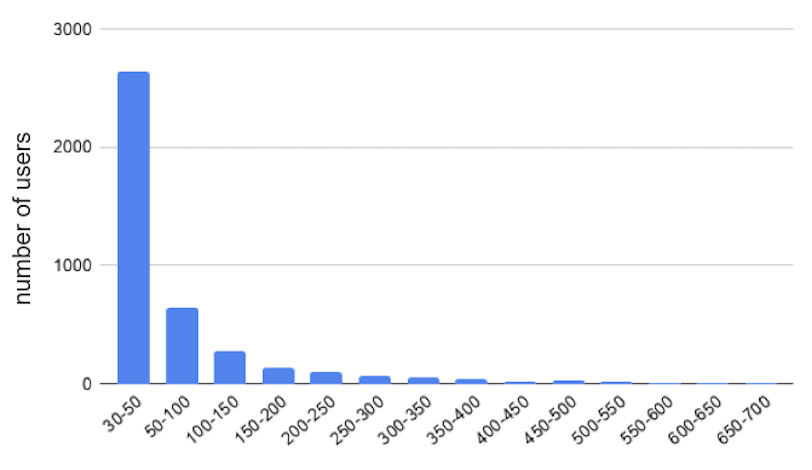
(a) Reviews per user

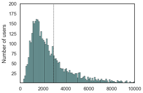
(b) Users’ vocabulary size

Figure 1: IMDb dataset statistics: (a) Distribution of the number of reviews per user. (b) Distribution of users’ vocabulary sizes. The vertical dashed line denotes the average vocabulary size

2.1 Missing popular terms

Our method would also consider popular terms that are missing from a user’s vocabulary. To motivate the use of missing terms, we detail here relevant statistics per user over the IMDb film domain. Figure 2(a) shows the distribution of missing domain popular terms from the vocabulary of review authors. The figure was calculated for users authoring more than 30 reviews, and it depicts the distribution of the number of popular terms, out of the most popular 1000 terms in the domain, that is missing from their vocabulary. Figure 2(b) shows the percentage of missing terms, normalized by the vocabulary size. The vast majority of users do not use terms that are among the top 1000 in the domain. The number of missing popular terms decreases as the vocabulary of the user is bigger. However, there is no linear relationship between them, and most users with 2000 and more terms in their vocabulary miss only 25% of the popular terms or less. This indicates that popular terms are prevalent in the use of most users. Hence, the lack of such use of a prevalent term should be indicative and distinct.

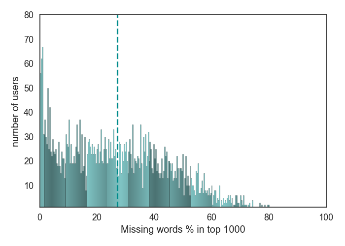
(a) Percentage of missing terms from top 1000

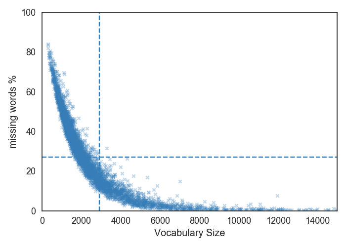
(b) Percentage of missing terms normalized by vocabulary size

Figure 2: IMDb dataset: missing terms in users’ vocabulary. (a) Distribution of missing top 1000 domain terms from users vocabularies. (b) Distribution of missing top 1000 domain terms normalized by the users’ vocabulary size.

3 Domain-based Latent Personal Analysis method

For a set of entities that constitute a domain, LPA intends to find the entities’ signatures, defined as the elements that make the entities unique and set them apart from the domain. In language, that would be the words that set authors apart from the domain. In music, signatures can be the songs that set a user apart; if the entities considered are countries, their signatures would consist of the songs that set countries’ listening habits apart. As the method’s insight arrives from languages’ characteristics, we describe it here using text and authors. To find how a person’s vocabulary differs most from the domain’s vocabulary, we need to establish which distance metric is best suited for the task.

Here, we will (1) explain the setup; (2) Devise criteria for choosing a distant metric for the method and explore which metric, out of four chosen candidates, is most suitable for our needs; (3) Demonstrate that the resulted entities’ distances from the domain’s vector are not an artifact of them being part of the domain but are significant, and also encode important information that can be utilized; (4) Devise a criterion for choosing signature lengths and construct LPA-signatures; (5) Give examples of the construction process for the Books and Social Media datasets, and also an example for non-text domains taken from the music industry.

3.1 LPA  setup

Here, we use the following definitions. Considering the used datasets, described in Section 2: Each book, chapter, or user’s reviews are entities in a domain. When referring to the Books dataset, an entity is either a book or a chapter, according to need. For the social media dataset IMDb, hereto referred to as Social Media dataset, an entity is a user, and the corresponding entity’s text is the aggregation of all the reviews written using a single user account. The collection of all the texts by all authors in each dataset is termed a domain document. Each entity’s text is termed an entity’s document. We take a Bag of Words (BoW) approach to deal with the unstructured text: tokenization, case folding and normalization, punctuation and stop-words removal, part of speech tagging. (We omit stop-words since we want the signatures to characterize the entities for explanatory and content-based characterization). We create a weighted vector for the domain and each entity’s document. The weighted domain vector is termed Domain Vector Rates (DVR). Each weighted entity’s vector is termed Personal Vector Rates (PVR). For the construction demonstration and definition we use the noun-terms.

3.1.1 DVR  construction

The weighted collection vector, DVR, is constructed out of the entire collection, the aggregation of all the domain entities. In the case of a book, the collection is the entire aggregated text of all the chapters. In the Social Media dataset, it is the entire text written in all reviews by all users considered in the domain.

To construct the DVR, we compute each word’s relative weight as its relative frequency out of all the domain words. For example, a word that took up 10% of all users’ BoW is assigned a weight of $0.1$. In the following toy example, we take a small part of the Social Media dataset to demonstrate the method setup. Table 1 depicts the elements, their global frequency in the collection, and their corresponding DVR  weights. The most popular word is ranked first in this list, etc.

Table 1: Toy example of a domain vector construction

Noun	Global frequency	Global probability
term	in collection	in collection
Film	1276332	0.0212
Movi	1117427	0.0184
Charact	406469	0.0067
Time	379878	0.0062
Stori	339747	0.0056

3.1.2 PVR  construction

Similarly, we construct a weighted frequency vector per entity. It should be noted that each entity uses a smaller vocabulary than the entire set of entities in the corpus. For example, if a book is a domain, and each chapter is an entity, the number of different words at each of the chapters is probably smaller than the number of distinct words in the book. Similarly, each user’s number of words in all of their reviews in the Social Media dataset is probably much smaller than the number of different words used by all of them together in what we term the domain. That is, most authors do not use every word in the DVR. However, we would like to compare their vectors with that of the domain. Therefore, we construct entities’ vectors as sparse vectors, containing null coordinates for words existing in the corpus but not in the entity’s writings. An entity’s PVR, therefore, is usually very sparse. An example of a few such random rows for our Toy example is shown in Table 2.

Table 2: Toy example of an entity vector construction

Word	Probability
favorite	0.546
drama	0.318
film	0.136
boat	Null (0)
brother	Null (0)

3.2 Distance metric selection

The choice of a distance metric is central to the method. If chosen correctly, then the elements most contributing to the distance of an entity from its domain are the ones that distinguish this entity. Per our discussion, these elements are elements that the entity contains much less relative to the domain and much more. Here, we use the Social Media dataset.

3.2.1 Distance metrics considered

Distance metrics attempt to formalize the natural properties of spatial distance. They are generally used to introduce a geometric structure to more abstract sets. For this research, however, we are not interested in such a geometric structure. Specifically, as we are always interested in the distance between two distinct points, and not in the shortest way to reach one from the other, we are willing to consider functions which do not satisfy the Triangle inequality. Such functions are called semi-metrics. However, here, we will informally use the term metric. We define here the distance metrics we chose. In Appendix B, we prove that each of our selected metrics is indeed a distance metric. Reviewing past research in the subject and related areas, we selected four candidates to serve as our metrics. In Appendix B, we show that each is a distance metric, i.e., fulfills the following criteria: non-negativity, symmetry, and identity of indiscernibles (proofs omitted from here for lack of space).

Rank Biased Overlap Distance (RBD)

Rank Biased Overlap, or RBO (Webber et al., 2010), assigns a similarity value to non-conjoint lists, i.e., lists which do not necessarily have the same items. RBO assigns a similarity value to two such lists by calculating their overlap over various segments of the lists. It is rank-biased because overlapping at the head of the lists contributes to the similarity value more than overlap at the tail. RBO itself is not a metric but a similarity measure. However, we can derive a distance metric from it, termed RBD, by defining $RBD=1-RBO$.

To calculate the RBO value of two lists $V_{1},V_{2}$, we first consider the intersection size between the lists over the first $d$ terms, i.e., how many elements appear in the first $d$ terms of both lists. We call this value $X_{d}$. We then define $A_{d}$, the agreement between the two lists over the first $d$ terms, as $A_{d}=\frac{X_{d}}{d}$. Note that $X_{d}\leq d$ and therefore $A_{d}\leq 1$. Then the RBO similarity measure of the two lists $V_{1},V_{2}$ is defined as follows:

$$RBO(V_{1},V_{2},p)=(1-p)\sum_{d=1}^{\infty}p^{d-1}\cdot A_{d}$$ (1)

Where $p$ is a parameter in the range $0<p<1$ which determines the weight given to the head of the lists - the closer $p$ is to zero, the greater the bias towards the head. The distance between the two lists is then $RBD=1-RBO$.

Cosine Similarity

Cosine similarity between two vectors $V_{1},V_{2}$ is defined as follows:

$$D(V_{1},V_{2})=\frac{V_{1}\cdot V_{2}}{\|V_{1}\|\times\|V_{2}\|}$$ (2)

Where $\cdot$ is the standard dot product, $\times$ is the standard multiplication and $\|v\|$ is the standard $L^{2}$ Euclidean norm.

$L1-Norm$

The $L1-Norm$  has been in use since at least 1757 when Roger Joseph Boscovitch used it for regression analysis. Since then, it has often been used in assessing the difference between discrete frequency distributions, making it a good candidate for our needs. For $V_{1}(x)$, $V_{2}(x)$ frequency vectors, we used a modified version of $L1-Norm$  distance such that the maximal distance between the lists is 1. Let $V_{1}$ and $V_{2}$ be non-conjoint lists, then

$$L_{1}(V_{1},V_{2})=\frac{1}{2}\sum_{x\in X}\arrowvert V_{1}(X)-V_{2}(X)\arrowvert$$ (3)

Kullback-Leibler Divergence (KLD) with a back-off

The Kullback-Leibler Divergence (KLD) (Kullback and Leibler, 1951) is a familiar statistical method for measuring the difference between two distributions $V_{1}$ and $V_{2}$. For two distributions, $V_{1},V2$, of a set of elements $X$, KLD is calculated by:

$$D([V_{1}\Arrowvert V_{2}])=\sum_{x\in X}\Bigg{[}\big{[}V_{1}(x)-V_{2}(x)\big{]}log\Big{[}\frac{V_{1}(x)}{V_{2}(x)}\Big{]}\Bigg{]}$$ (4)

KLD was designed for two distributions of the same set of elements, as it assumes that for every $X$, both $V_{1}(x),V_{2}(x)$ are non-zero. In our case, however, most users (entities) do not use the domain’s entire vocabulary. That is, for some elements $x\in X$ we have $V_{1}(x)=0$.

To account for the large variance in vector lengths and counterbalance the domain’s long-tail of rare words, we use a variant, the KLD with a back-off model, defined in Bigi (2003). This variant assigns missing words a constant value $\epsilon$. This value is chosen to fulfill two requirements: it must be less than the frequency of a single word in the entire domain (corpus), and it must be large enough so that KLD still gives results in the range $[0,1]$. In effect, we expand the user’s (entity’s) vector from a sparse vector to one containing a positive value in every coordinate. This, however, also means that the extended vector, $V_{e}$, is no longer a probability vector - the sum of all coordinates is now larger than 1. We correct this by multiplying all non-$\epsilon$ frequencies by a normalization coefficient $\beta$. This normalization coefficient is given by the formula $\beta=1-N\epsilon$, where N is the number of words missing in one vector compared to the other.

Thus, an extended frequency vector $V_{e}$ is defined by:

$$V_{e}(t_{k}\|d_{j})=\left\{\begin{array}[]{lr}\beta V_{1}(t_{k}\|d_{j})&t_{k}\in d_{j}\\ \epsilon&\quad\textit{otherwise}\\ \end{array}\right\}$$ (5)

Where $d_{j}$ is the original vector before the extension, not containing missing words.

We can verify that this is indeed a frequency vector: let $X$ be the set of all indices in the vector, $K\subset X$ the set of all non-$\epsilon$ indices, i.e. those that had non-zero value in the original vector and $N$ the number of missing words, i.e. how many coordinates have an $\epsilon$ value. We then have

$$\sum_{x\in X}V_{e}(x)=\sum_{x\in K}V_{e}(x)+\sum_{x\not\in K}V_{e}(x)=\sum_{x\in K}\beta V_{1}(t_{k}\|d_{j})+\sum_{x\not\in K}\epsilon$$

but since $V_{1}$ is a frequency vector, $\sum_{x\in K}V_{1}(t_{k}\|d_{j})=1$ and we therefore have

$$\sum_{x\in X}V_{e}(x)=\beta\sum_{x\in K}V_{1}(t_{k}\|d_{j})+N\epsilon=1-(N\epsilon)\times 1+N\epsilon=1$$

We refer hence-forth to the (Bigi, 2003) version as $\textit{KLD}_{\varepsilon}$.

3.2.2 Selection criteria

We compare here the performance of the distance metrics according to four criteria. A distance metric used in our method should:

1. Provide wide distribution of results when calculating entities’ distance from the domain, indicating that the metric is sensitive enough to small differences between entities. We used Kurtosis as an indicator of the distribution’s width. Kurtosis is a statistical measure that defines how the tails of a given distribution differ from the tails of a normal distribution. A wide distribution should have relatively small Kurtosis Excess.

2. Missing popular words should contribute to the distance.

3. The distance function should be more sensitive to differences at the head of the vector (the relatively few, more popular words) than at its tail. Vocabularies tend to have a long-tail distribution, and this criterion ensures that many minor differences in the tail would not overshadow the few, more significant, differences at the head.

3.2.3 Criterion 1: small kurtosis excess of distances from the DVR

We calculate each entity’s distance from the DVR  in each of the four proposed metrics.

Table 3: Criterion 1 results: distance distribution statistics including Kurtosis Excess for each of the distance metrics used

Metric	Min	Max	Average	Std.	Median	kurtosis Exc.
RBD	4.49E-08	02.05E-06	8.481E-08	2.819E-08	7.95E-08	6.51
1- cos.-sim.	0.00034	0.04561	0.003039	0.00246	0.00249	2.8
$L_{1}$	0.237383	0.775756	0.435991	0.069562	0.433481	-1.2
$\textit{KLD}_{\varepsilon}$	0.035	0.861	0.223	0.114	0.203	1.48

Table 3 depicts the distance distribution statistics for each of the distance metrics. The distribution is the distribution of users’ vectors’ distances from the DVR. Of the four, RBD (recall that $RBD=1-RBO$) has the highest kurtosis excess and the narrowest distance distribution. Therefore, we reject RBD and continue with the other three: $1-\textit{Cosine similarity}$, $L1-Norm$ and $\textit{KLD}_{\varepsilon}$.

3.2.4 Criterion 2: contribution of missing popular items to the distance

To measure the contribution of missing popular words, we select the most popular 1,000 terms in the domain. We then calculate each entity’s distance from the domain, based on these 1,000 terms, and determine the contribution of each user’s missing words to that distance, as calculated by the three remaining distance metrics. $1-\textit{Cosine similarity}$  fails to measure this contribution, as only terms that appear in both vectors with values greater than zero add to the distance. Hence, we reject the use of $1-\textit{Cosine similarity}$, and are left with $L1-Norm$  and $\textit{KLD}_{\varepsilon}$.

3.2.5 Criterion 3: distance function sensitive to differences in the head and less sensitive to differences in the tail

To test the compatibility of the remaining metrics to this criterion, we took the complement of the vectors from the previous one - here, we only considered the terms after the $1,000$ most popular. Figure 3 depicts the distributions for this criterion.

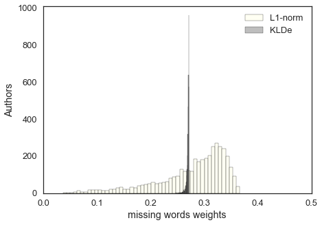
Figure 3: Criterion 3: the contribution of missing words in the tail to overall distance under $\textit{KLD}_{\varepsilon}$  and $L1-Norm$.

The results show that $L1-Norm$  is biased to the right (larger distance). This is consistent with the fact that it correlates with the entity’s vocabulary size - an author with a large vocabulary will have fewer missing words and, therefore, be closer to the DVR. As $L1-Norm$  assigns a high value to rare missing terms, it fails this criterion, and therefore $\textit{KLD}_{\varepsilon}$, which provides a wide distribution and a balanced average, is our chosen metric. We then wrap-up the method construction by utilizing $\textit{KLD}_{\varepsilon}$  as the chosen metric.

3.3 Validity of the $\textit{KLD}_{\varepsilon}$ distance as an attribute of an entity

We continue to validate that an entity’s distance from the DVR is not merely an artifact of the entity being a sample from the domain. We choose 210 users from the Social Media dataset; each contributed 100 to 120 film reviews of different lengths. We term them ’authentic’ users. We then create 210 virtual users, whose text was chosen randomly from the dataset. We select randomly for each virtual user between 100 to 120 reviews at random from the dataset. We then create signatures for both authentic and virtual users and compute the distances. Let $f_{n}$ be the distribution of distances of normal users from the DVR. Let $f_{v}$ be the distribution of distances of virtual users from the DVR. Then, we hypothesize that there is a significant difference between $f_{n}$ and $f_{v}$. We use an independent-sample t-test to compare the two distributions and find a significant (t(418)=-59.05, p=0.00) difference between the authentic users (M=0.459, SD=0.11) and the virtual users (M=0.919, SD=0.14). This allows us to reject the null hypothesis and confirm that authentic authors’ distance distribution is significantly different from that of a randomly selected text of similar size.

In summary, LPA distances are a newly found attribute of the entities. An entity’s LPA distance is a measure of how similar is its distribution to that of the domain’s. Our criteria require that entities with a similar head of distribution to that of the domains’ are closer to the domain (short distance) than entities that differ substantially in the elements constituting the head of their distribution. When the entities are users and the elements are terms, users who use the popular domain terms have a shorter distance to the domain than those who do not. We will discuss the outcomes of this observation in Section 4.2.

3.3.1 Constructing LPA signatures

We have established a distance measure based on how an entity is different from the domain. However, as we will show here, for many purposes, entities can be represented by their signature, a vector representation constructed of the top N terms most contributing to the entity’s LPA distance from the domain. That is, what makes entities unique, and sets them apart from the domain. Utilizing the entity’s PVR  distance from the DVR, we continue to form an entity’s signature as the N-words which contribute most to this distance. Two points should be noted regarding this definition: i) A signature is not a trait of a particular text, but a text relative to another text. A signature is a vector representation constructed out of the N-words, which most differentiate a given text from a given domain. So while we will use the term signature here, it should always be considered relative to a specific domain. ii) A signature might contain elements that do not exist for the entity; in our case, words that are not in the author’s vocabulary. If a specific word is prevalent in the domain but absent from an author’s writings, that tells as much about the author as if a word was very infrequent in the collection but very popular in the author’s writings.

Working set size

Works using word frequency vectors share a common difficulty in determining the working set’s size. Bigi (2003), in her KLD back-off model work, used a working set of 500 terms for text categorization. Baker and McCallum (1998), likewise working on text classification, have achieved 66% accuracy with the top 500 words per text. Researching corpus similarity measures,  Kilgarriff and Rose (1998) have achieved the best results when using the 320-640 most popular terms.  Ntoulas et al. (2006) used the most frequent 500 words to detect spam webpages. They Found that 500 words were enough to extract 75% of the relevant information. By the very definition of a signature, the N-words which contribute most to the user’s distance from the DVR, each additional word should have a diminishing return on the distance. Therefore, we want to use as few words as possible while still retaining the essential characteristics reflected by the distance. We proceed to show that $N=500$ indeed justifies these claims.

We analyzed the two datasets, Books and Social Media. Table 4 details the average calculated contribution of the top furthest 50, 100, 500, and 1,000 words to the distance in two datasets. In both datasets, the top 500 words contribute around 50% of the distance. A further increase to the top 1,000 words yields an increase of only 10% of the total distance. When considering the diminishing return of additional words, we find that the diminishing return was less than one percent around the $100_{th}$ word. The exact length of the signature is then a trade-off between computing effort and precision. Based on the above-described findings, we also set the signature size to 500, i.e., $N=500$.

Table 4: The average contribution of the top 50, 100, 500 and 1,000 words to a user’s vector distance from the DVR

Dataset	50	100	500	1,000
Social Media	16.32%	22.70%	45.84%	55.11%
Books	19.87%	29.28%	56.80%	66.20%

We further see that the first $N=500$ terms contribute to the distance differently to different entities. For some, the top N words contribute 70% and more of the measured distance. To others, the top N words contribute less than 50% of their $\textit{KLD}_{\varepsilon}$  distance. Specifically, we find that the top N words contribute less to entities closer to the DVR  and more to distant entities. In other words, the more distinct a user’s style is, the more their signature is representative of that style. This result implies that taking the top N terms gives a robust result across all users.

Latent terms contribution to the signatures

Using our Books dataset, we create signatures for 1,118 chapters relative to the entire dataset. We measure the distance of these signatures from the DVR  and examine what percentage of each signature’s distance is contributed by words existing in the user’s vocabulary and what percentage is contributed by words missing from it. Figure 4 shows the correlation.

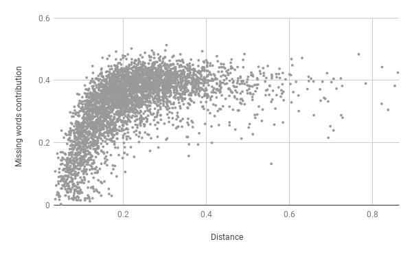
Figure 4: Correlation between entity’s distance from the DVR and the contribution of missing terms to the distance

As expected, the results show a clear trend. That is, for distant entities, a larger percentage of the distance was contributed by missing words.

3.4 An entity’s LPA signature: the essence of an entity’s difference from the domain

We demonstrate LPA-signatures  construction with Daniel Defoe’s novel Robinson Crusoe (1719) and the Social Media dataset. We also give a brief example of how LPA  can be used in various domains using a dataset of song popularity per country released by Spotify in 2017.

The story of Robinson Crusoe is of an Englishman, castaway on a deserted island for 28 years, later saved to return to civilization. He returns accompanied by Friday, an escaped prisoner he rescued.

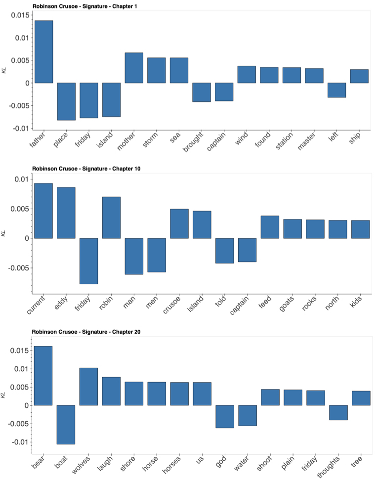
(a) Top terms in the signatures of Chapters 1, 10, and 20, corresponding to the first chapter, half-way, and the last one.

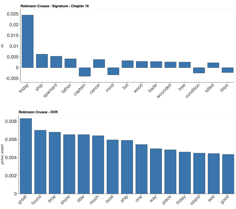
(b) The lower panel depicts the novel’s top DVR terms. On the upper panel, the top terms from Chapter 16’s signature. In this chapter, Friday and Robin rescue Friday’s father and plan to leave the island.

Figure 5: Daniel Defoe’s novel Robinson Crusoe: DVR, LPA-signatures

In the construction of this novel with LPA, the entities are the chapters, and the domain is the book. Thus, the DVR shows the novel’s term frequency, while the LPA-signature of each chapter depicts the terms that most set the chapter apart from the novel. Figures 5a, 5b, show the domain’s top DVR terms and the top terms of the LPA-signatures  of chapters 1 (the first), 10, 16, and 20 (the last). The novel’s top twenty terms consist of prominent plot-related terms such as shore, boat, ship, island, sea, Robinson’s companion Friday, and God. In chapter one, the parents play a central role, as well as the sea. In chapter ten, other people (man, men) are discussed much less. Instead, the parrot echoing Robin’s name is prominent, as is Robin’s mishap in the stream. Chapter 16 is dominated by Friday, the Spaniard, and the term ”mind” is underused. The final chapter, 20, concentrates on a fight on the shore with a bear. The prominent missing terms are boat, God, water, thoughts. The term laugh, however, appears much more than in the rest of the book.

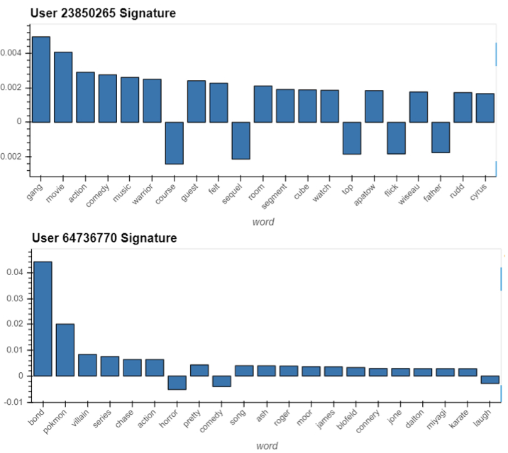
Figure 6: LPA-signatures  of two users from the Social Media dataset, a film review platform. Signatures contain both overused and underused terms.

For the Social Media dataset, we give the LPA-signatures of two randomly selected users. Figure 6 Shows their signatures. We see on the upper panel a user discussing movies, thoughts, and how the user ’felt’. They talk less about cast, script, and horror films than is common. On the lower panel, we see a Bond films’ reviewer who avoids horror and comedy and mentions the word ’laugh’ less than is common.

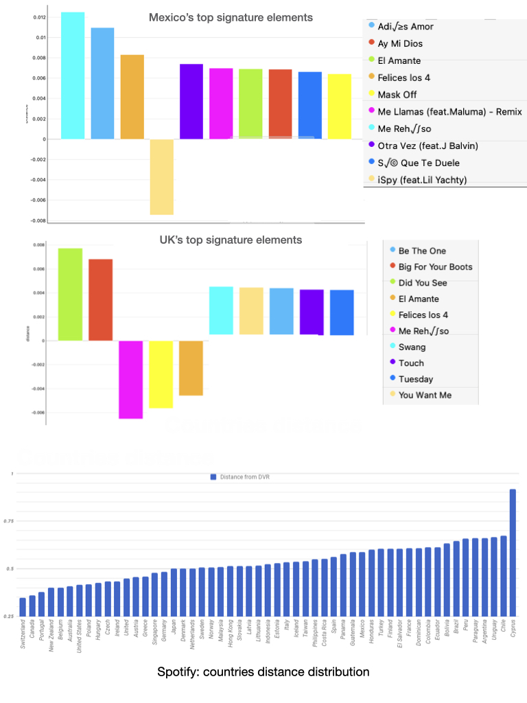
Figure 7: LPA-signatures for the music domain: an example over a Spotify dataset from 2018. The lower panel gives the distances of countries from the DVR. The upper panel details the top elements in the LPA-signatures for Mexico (left upper panel) and the UK (right upper panel). The UK is closer to the DVR, and the head of its distribution is similar to the top world view; hence its signature contains subtler changes. In Mexico, local music is more favored; hence Mexico is more distant, and its signature weights are larger than the UK’s.

To demonstrate how LPA can be used in non-textual domains, we take as an example a dataset of songs from Spotify from 2017. The dataset contains all songs streamed in that year and their listening frequency in each country. To create the DVR, we created a vector frequency of the aggregated countries’ lists, obtaining a world frequency view of songs’ popularity. We then create the LPA-signaturesfor the countries. Figure 7 shows The results. The lower panel depicts the distance from the DVR  and relative stream size for each country. Countries that listen more to popular music are closer to the DVR. Examples of these are Canada, Switzerland, and Australia. These countries’ signatures are characterized by small differences in listening habits to hit songs. Countries distant from the DVR are these in which local music is preferred, for example, Turkey or Uruguay. On the upper panel, we see the signatures of two countries with a roughly equal volume of listened tracks, Mexico and the UK. Mexico, the distant one, has a signature that is dominated by popular local music tracks. The UK is closer in distance to the world and has a signature that is dominated by subtle differences from the DVR.

3.5 LPA calculation: a fast and slim process

Let N be the total number of terms, or elements, in the domain, and Q the total number of entities in a domain.

Memory considerations: To construct LPA-signatures, the algorithm requires that entities’ vector lengths be identical to that of the DVR’s. The total memory size for this phase is $3\cdot N\cdot Q$, considering each element has a corresponding weight, and after calculating the $\textit{KLD}_{\varepsilon}$ distance, a sign. However, the working set size consists of 500 terms (signature size) per entity, and thus the memory requirement for the LPA-signatures  is merely $500\cdot Q$.

Execution time considerations: There are two phases of computations for the LPA-signatures construction. In the setup phase, the $\textit{KLD}_{\varepsilon}$ distance between each entity and the DVR is computed. The distance between each entity’s vector and the DVR is given by Equation 4, and requires one pass over the vectors’ length while computing a log function. Hence, computing the distances is of O(N) complexity. In the second phase, the LPA-signatures are computed by choosing the top 500 terms.

Similarity time considerations: Computing the similarity between any two entities’ signatures requires an $L_{1}$ computation over 500 elements. That is, it is $O(Q^{2})$. When used as a similarity measure, that is, finding similar signatures, LPA requires computation power of the order of the number of entities considered to the power of 2 (that is $Q^{2}$).

4 LPA’s uses

LPA  creates two representations for each entity in a specific domain: the entity’s distance from the domain and its signature (vector representation) in the domain.

Here, we show that an entity’s distance from the domain is a measure of its uniqueness. In the case of text, it is a measure of style. When the domain consists of a single author’s writings, each sample’s distance (that is, an LPA entity) from the domain is small. However, when the domain consists of various authors’ writings, a relatively small distance of a sample text (and LPA entity) is an indication that multiple authors are responsible for that text, perhaps pretending to be a single author.

The signatures are a vector representation of an entity in a domain. Hence, in the case of text and authorship, when two entities’ vectors’ representations are very similar, it is an indication that a single author wrote both text samples (entities). We further show that the representations of two chapters of the same book are closer to each other than to chapters’ representations of other books by the same author. Further, when the domain consists of various authors’ writings, the similarity between books’ vector representations (LPA-signatures) is a measure of styles’ closeness.

We conclude this section by considering the amount of information needed to produce reliable signatures by comparing sampled chapters’ signatures to complete chapters’ signatures.

Here, we will mostly use the Books dataset since this is a fully labeled dataset: each chapter is part of a book written by a single author. As will be discussed, we consider each book both as a domain and an entity, dependent on the context. Thus, conditional on the experiment, either the book is an entity, or a chapter is an entity. When the chapters are entities, the experiments can contain hundreds of entities.

4.1 LPA  entities’ distances as a measure of authorship

Here we show that the LPA’s entities distances can identify authorship. We show that book chapter entities are closer to their book’s DVR than to arbitrary books’ DVR’s. We create arbitrary books, which we term ’virtual’ books, by randomly choosing chapters from various books written by different authors. We construct each book as a DVR  and its sample chapters as PVR’s. We further create virtual books’ DVR’s and the randomly selected chapters as PVR’s. Hence, we hypothesize that the mean distance between the chapters’ PVR  and the authentic book DVR is significantly smaller than that of chapters’ PVR  and virtual books’ DVR. We perform a sequence of three experiments, controlling first for the book and chapter lengths, and with each experiment, we relax length restrictions to see the validity of the method for texts of different sizes, adding a sensitivity test. Table 5 depicts our results. The results are averaged over 30 real books and 30 virtual books. Each real book contains between 7 to 61 chapters. Virtual books were created with a randomly chosen number of chapters from the pool of real books. Each virtual book contains 19 to 31 chapters.

Table 5: Distance as a measure of authorship: validation and sensitivity

Experiment	Description	Average	Median	Std.
Normalized baseline	Distance of a 1,000 words chapter from a 10-chapter authentic book	0.306	0.304	0.057
	Distance of a 1,000 words chapter from a 10-chapter virtual book	0.717	0.511	0.398
Normalized chapters	Distance of a 1,000-words chapter from an authentic book	0.369	0.379	0.061
	Distance of a 1,000-words chapter from a virtual book	0.78	0.654	0.162
No normalization	Distance of a chapter from an authentic book	0.474	0.453	0.121
	Distance of a chapter from a virtual book	0.667	0.654	0.162

The corresponding values of independent two-sided t-tests are the following: Normalized baseline: T(18)=3.2326, p=0.0046; Normalized chapters: T(58)=13.004, p=0.0001; No Normalization: T(58)=5.228, p=0.0001. Hence, we can reject the null hypothesis. Hence, the distance of chapters’ PVR  from their authentic books DVR is significantly smaller ($p<0.005$) than that from their distance to the virtual books. This also holds when text length is not normalized.

4.2 Using LPA’s entities distances to detect that multiple authors wrote a single piece of text

Recall that at the heart of the LPA construction method lies the assumption that a domain’s long tail distribution is the sum of individual language usage patterns manifested in personal vocabulary distributions. The head of the DVR then can be seen as a superposition of the heads of the entities’ vocabularies distributions. As discussed in the Introduction, this is an underlying, sometimes latent, assumption in many language models that identify topics using prominent terms’ frequencies.

Building on this motivation, we hypothesize that text’s vocabulary frequencies written by multiple authors will resemble the DVR’s frequencies, especially in the head, as both vectors result from a superposition of individual terms’ usage patterns. Recall that the head of the DVR reflects the typical use of popular terms in the domain. LPA identified the personal differences of an individual as their style. Hence, we can assume that when the head of an entity’s distribution is very similar to that of the domain, it results from a superposition of several authors’ styles. Hence, the hypothesis is that entities’ text, when the entities are very close to the domain, is written by multiple individuals.

How do we show it? To that end, we return to the process we have used before of creating virtual books. Recall that a virtual book is a collection of chapters randomly chosen from other authentic books and collected together as a collection we term ’virtual book’. Thus, taken together, we have a collection of authentic books and virtual books. Thus, our domain is the entire Books dataset, and each authentic book and virtual book is an entity. When constructing the DVR, we consider only the authentic books (As the DVR is constructed in a bag-of-words approach and the virtual books are composed of chapters from the authentic books, both DVR’s, for the virtual books and the authentic books, are identical).

We then compare the distances of authentic books from the DVR  to that of the virtual books. Figure 8 shows the distribution of distances from the DVR  for both virtual and authentic books.

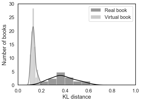
Figure 8: Distances from the DVR  for both authentic books and virtual books computed over the Books dataset

We find that the virtual books are both much closer to the DVR  and present a much narrower distribution. This indicates that distance can be a good indicator of whether a specific text was written by multiple authors and is thus a superposition.

4.3 Similarity between LPA-signatures as a measure of context-based authorship attribution

Here, we define a domain as ’19th century-novels’ and create a subset of the Books dataset as a domain. The subset contains nine books authored by different authors. Three of the books were authored by Jane Austen, and two books by the Bronte sisters, each a book. The other novels were authored by Lewis Carol, Charles Dickens, Mark Twain, and Arthur Conan Doyle. We create the DVR of all nine books and the corresponding LPA-signatures for each novel. We then compute the similarity between the signatures.

Computing the similarity is not trivial once missing or underused elements are included in the signatures. LPA-signatures  have both weights and signs. A term missing from the entity’s vector but frequent in the domain can be highly important in the user’s signature, resulting in a high absolute weight, but with a negative sign, indicating that it is missing. When comparing signatures, we would like to take into account the sign. Consider two entities with the same term in a high place in their signature; One uses it more than the typical domain usage, and the other never uses it; This difference should contribute significantly to their distance. Hence, to compare, we add one to all the absolute weights that reference a term with a positive sign in the signature and subtract one from the absolute weight of terms that have a negative sign in the signatures, and then compute the distances using a simple $L1-Norm$ metric.

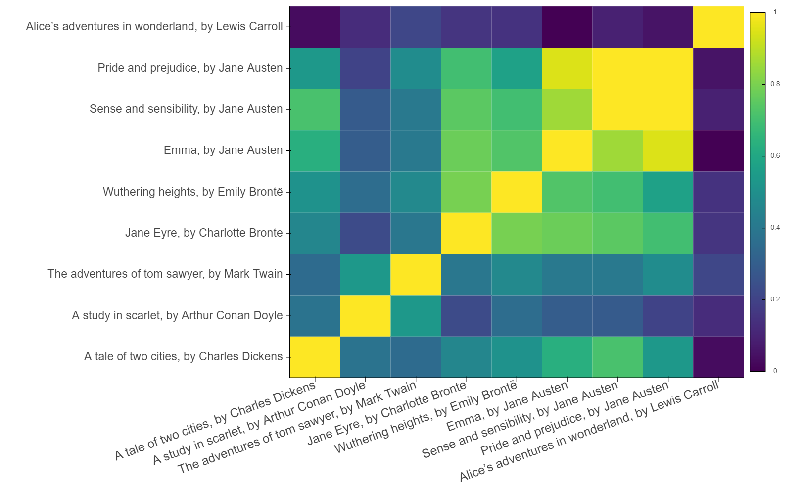
Figure 9: A similarity heatmap (1-distance) between nine 19th century-novels’ signatures.

Figure 9 depicts a similarity heatmap (1-distance) between the novels’ signatures. that is, two novels’ signatures are very close if the corresponding similarity is one. All three Jane Austen books have similar LPA-signatures, with Pride and Prejudice and Sense and Sensibility closer to each other than to Emma. The novels by the sisters Bronte have more similar signatures than any other two novelists; however, their signatures are also relatively close to those of Jane Austen’s novels. Interestingly, the signatures of the novels Sense and Sensibility and A tale of two cities by Dickens are also somewhat close. The most different signature is that of the novel Alice’s adventure in wonderland by Lewis Carrol.

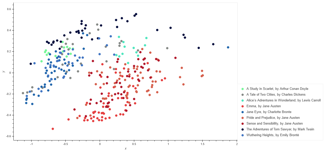
Figure 10: A PCA of the distance matrix table of all 19th-century novels’ chapters. The first dimension accounting for 28% of the variance, the second for 8%.

To identify the differences between personal styles more clearly, we increased the resolution by treating each chapter of the 19th century-novels as an entity. Each chapter out of the 360 considered is a sample of its authors’ writing, and we, therefore, wanted to test to what extent LPA  would identify and differentiate individual authors’ writings when the chapters are the entities. We created a distance matrix table of all chapters LPA-signatures. A PCA of these distances, depicted in Figure 10 accounted for 36% of the variance in its first three dimensions, with the first dimension accounting for 28%. Here, we find that the writings of Jane Austen diverge from the rest, as are the styles of the Bronte sisters and Dickens in a Tale of two cities.

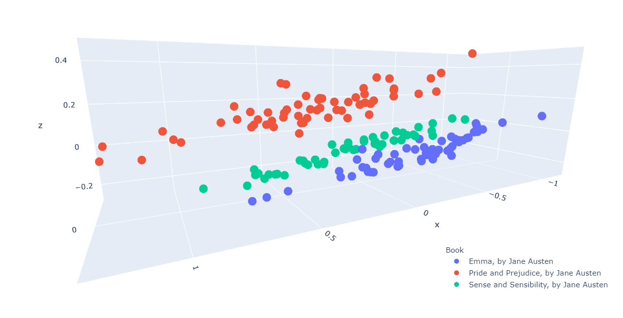
Figure 11: A PCA of the distance matrix table of Jane Austen’s three novels’ chapters. The first dimension accounts for 25.6% of the variance, and two more dimensions added together 7% to a total of 32.5% of the explained variance

Jane Austen’s novels show high similarity. To further drill down into it, we created a DVR and LPA-signatures out of the three novels’ chapters and created a corresponding distance matrix. Figure 11 depicts the PCA of the distance matrix. The first dimension accounts for 25.6% of the variance, and two more dimensions added together 7% to a total of 32.5% of the explained variance. There is a clear separation between the three novels, with Pride and Prejudice diverging from the other two novels.

Thus, while LPA  captures a personal style and can be used as an authorship-attribution method, its content-based approach enables it to differ between the same author’s writings. That is, LPA enables a context-based author attribution.

4.4 Entities required sample size

To understand the limitations of LPA, we conduct the following experiment to identify the minimal amount of text needed to identify a signature correctly. We consider each book as a domain and each chapter as an entity in the domain. The optimal chapters’ signatures are obtained when the entire chapter is considered. However, it could be that the prominent terms that set a chapter apart from the domain can be determined using less information. We term the signatures obtained with entire chapters optimal signatures and conduct a set of experiments to find the minimal amount of information needed to obtain a close-to-optimal signature.

For each book $i\in$ the Books dataset, we find the average length of a chapter in a book, $X_{i}$, and vary a sample length, $j$ in the range $L={0.1X,0.2X,\ldots 1.2X}$. As $X_{i}$ is an average chapter length, some chapters will be shorter than $X_{i}$ and some longer. For each sample length $j\in L$, we create a DVR and signatures for book $i_{j}$, that is, the sampled book $i_{j}$ that consists of chapters of length $j$. For example, assume $j=0.1X$. Each entity (chapter) is a frequency vector formed from the chapter sampled with the first 10% terms (10% of the average chapter length). The DVR is the aggregated frequency vector of the combined entities, and the signatures consist of the terms most distancing the entities (sampled chapters’ vectors) from the DVR. We then compute for each entity’s signature its $L_{1}$ distance from the corresponding chapter’s optimal signature. The number of terms in each book corresponds to the number of nouns and adjectives.

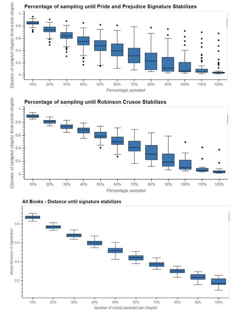
Figure 12: Sample size that yields a signature close to the one received with full information. Upper panel: Pride and Prejudice; Middle panel: Robinson Crusoe; Lower panel: Average over the entire dataset. Each Box plot corresponds to the average over the 30 books, a total of 943 chapters.

Figure 12 shows the Box plot of the distances of the sampled chapters per the Novels Pride and Prejudice, Robinson Crusoe, and for the entire Books dataset. The novel Pride and prejudice consists of 61 chapters with an average chapter length of 780 terms. The life and adventures of Robinson Crusoe contains 20 chapters with an average length of 2060 terms. The upper two panels show the average distance between the sampled chapters’ signatures and the optimal signatures for each sample length. The signatures are close to the optimal signatures for both books when we get to a sampling that corresponds to 0.8 of an average chapter’s length. The lower panel depicts the average result over all the books, i.e., an average of averages. There are thirty books and a total of 943 chapters. In each experiment, we sample the chapters ten times on different lengths and compute the distances’ average for all sampled chapters. Thus, each point is an average of 30 averages, each taken roughly over 31. 4 chapters. Books differ in their number of chapters and chapters’ length. However, on average, the signatures become close enough to the optimal when we take 0.8 of the average chapter length. In summary, the signatures are more accurate the more information is used.

5 LPA in a social media domain

We continue to evaluate LPA’s performance over a large-scale real-world social media dataset in the movies’ domain. Here, we use the data from the IMDb review-platform site. It offers an opportunity to evaluate the performance of LPA  on a domain-based online free short text, and in particular, to identify two types of impersonation.

We identify two types of inauthentic users in a social media domain. One is multiple virtual personas (recently referred to as Sockpuppets when the accounts are used for various goals  (Kumar et al., 2017)), which are multiple user accounts operated by the same person. The other is what we term front-users, a single virtual persona operated by multiple people. LPA  lends itself to find front-users. Its definition comes from finding the DVR as the superposition of different styles. Hence, as we have shown in Section 4.2, accounts that are also a superposition of several styles will be typically closer and similar to the DVR.

We start by evaluating the capabilities of LPA  to identify the first type of impersonation, two user-accounts with the same author. Recall that LPA  is an unsupervised method that creates vector presentations (signatures) for entities (users) in a domain, unlike current learning-based methods for authorship attribution in the wild (Abbasi and Chen, 2008; Koppel and Winter, 2014). We randomly choose 1000 users, each having between $4000$ to $7300$ words in all of their reviews combined from IMDb. The text of 10 randomly chosen users out of 1000 is halved, and two users are created from it, resulting in 1010 users. In the baseline method, we create the TFIDF  vectors for all 1010 users and compute the cosine similarity between all the vectors.

In our method, we create a DVR from the text of the 1010 users and compute their signatures. We then compare the signatures of all the users to each other ($510050$ comparisons). In Section 4.3, we have established that texts written by the same author have relatively closer signatures than to other arbitrary texts and described how we compute the distance taking into account that the same term can be either missing or over-used by two users. Recall that in LPA, signatures have both weights and signs. A popular term missing from the user’s vocabulary can be highly important in the user’s signature, resulting in a high absolute weight, but with a negative sign, indicating that it is missing. We use for comparisons the algorithm described in Section 4.3. To determine what relatively close means, we define a threshold as follows. We compute the average distance between all pairs, $\sigma$, with $\mu$ corresponding to the standard deviation. We then set the threshold to $\sigma+r\cdot\mu$, where $r=1\ldots 4$ in the different experiments. We determine that two user accounts have the same author if the distance between the accounts’ signatures is lower than the threshold. We can expect that a lower threshold increases the precision but decreases the recall.

Table 6: Authorship Attribution: LPA vs. baseline

Threshold	Baseline			Our method
	Prec.	Recall	F1	Prec.	Recall	F1
Avg - 1 std.	0.96	0.5	0.65	0.87	1	0.93
Avg - 2 std.	0.98	0.68	0.8	0.96	1	0.98
Avg - 3 std.	0.98	0.77	0.86	0.99	1	0.99
Avg - 4 std.	0.99	0.83	0.9	0.99	1	0.99

Table 6 details the results of the comparisons for both the baseline method and our method for the four threshold values. Our method outperforms the baseline in all cases. It always determines correctly the users that their text was halved as being the same author, with very low false-positive values, i.e., users that are mistakenly considered the same author.

5.1 Finding multiple personas (Sockpuppets) in big-data

Multiple virtual personas are several accounts operated by the same author, also termed Sockpuppets. As such, we expect them to have relatively close signatures in the domain. Continuing from above, we employ the method here over the entire Social Media dataset to find multiple users that belong to the same author on the Social media dataset. Our dataset contains $N=3969$ users, yielding $N^{2}=7,874,496$ comparisons. Our method computes the $L_{1}$ distance between them, and hence computation-wise takes $O(N^{2})$ time complexity over a memory requirement of $O(k\cdot N)$, $k=500$ terms. Table 7 details the number and percent of users our method identifies as multiple personas - i.e., their signatures are close to each other. We compute signatures as close using four different thresholds: one std, two std, and up to four std. ’s below the average.

Table 7: Social media dataset Sockpuppets results

Threshold	User pairs suspected as Sockpuppets	Percent
Avg - 1 std.	1,180,261	14.988%
Avg - 2 std.	336,173	4.269%
Avg - 3 std.	86,975	1.104%
Avg - 4 std.	21,996	0.279%

We conducted manual verification for a randomly chosen number of suspected users from this group (Avg - 4 std.). We found corroborating evidence from their personal information that the same person operates the accounts. For details and the full list of sockpuppets see https://www.scan.haifa.ac.il/post/domain-based-latent-personal-analysis-lpa-and-its-uses.

5.2 Finding front-users in big-data

The second kind of impersonation we are trying to identify is front-users, one virtual persona operated by multiple people.

Similar to our finding in Section 4.2, we find here front-users in a real-life dataset, our Social media dataset. To identify front-users, we compare the distance of the $3970$ users to the DVR. We expect a front-user’s vector to be relatively close to the DVR. We define the threshold as follows. We calculate all users’ distance from the DVRand find the average and standard deviation. We then define a lower threshold, e.g., a standard deviation under the mean. Any author whose vector’s distance is lower than this threshold is considered a possible front-user. We find that the average distance is 0.223 (Median: 0.203), with a standard deviation of 0.114 (the distance distribution is right-skewed). We consider users whose distance is not more than one standard deviation below the average, that is, their distance is below $0.109$, as suspected front-users. In our sample, $532$ users fit this criterion. Figure 13 shows the distribution of the users’ distances.

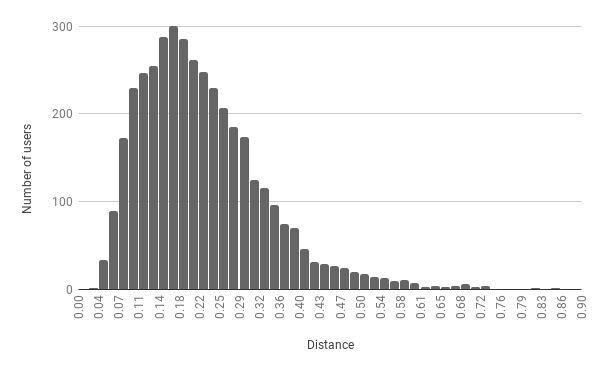
Figure 13: Distribution of Social media users’ distances from the DVR

To find evidence supporting our findings, we explore these users’ temporal rates utilizing visual temporal analysis and temporal measures. We are particularly interested in two parameters: i) the number of active days, and ii) maximum posts per day. To find a non-normal activity pattern, we disregard periods of inactivity. This allows us to depart from a timeline view and present a view that concentrates on periods of activity. We can thus easily detect peaks of extreme activity, which indicate inauthentic usage. Imagine, for example, that we find on the Social media dataset a user who has not been active for two months and then posted 60 reviews in one day. While the average would be one review per day, which is not suspicious in itself, it is evident that the user had not watched and reviewed 60 movies in one day. Alternatively, imagine a user who has been active entirely consistently every day, posting precisely one review every day. That, too, is inconsistent with normal human behavior, characterized by bursts of activity (Barabasi, 2005). We find these two patterns visually with Activemap (Ben-Shoshan and Mokryn, 2018), a Treemap visualization designed to highlight two types of outliers on social media: contributing users with a substantial amount of contributions or with extreme activity peaks. We Visualize the $532$ suspected front-users with Activemap, allowing us to quickly identify that many show a larger than normal activity volume either over the entire period or during specific days. Considering these are reviews for films, it is improbable, for example, for one user to write fifty such reviews during a single day, as is the case for some.

We continue with the temporal validation to quantify deviations from normal behavior patterns. We are particularly interested in two parameters: i) the number of active days, and ii) maximum posts per day. As we are interested only in days of activity, we disregard periods of inactivity. This allows us to depart from a timeline view and present a view that concentrates on periods of activity. We can thus easily detect peaks of extreme activity, which indicate inauthentic usage. Imagine, for example, that we find on the Social media dataset a user who has not been active for two months and then posted 60 reviews in one day. While the average would be one review per day, which is not suspicious in itself, it is clear that the user had not watched and reviewed 60 movies in one day. Alternatively, imagine a user who has been active consistently every day, posting precisely one review every day. That is inconsistent with normal human behavior, which is characterized by bursts of activity (Barabasi, 2005). Therefore, we are interested in two kinds of users - those who consistently post a large number of reviews or those with extreme peak activity.

We visualize the suspected front-users activity utilizing Activemap (Ben-Shoshan and Mokryn, 2018), a Treemap visualization designed to highlight two types of outliers on social media: contributing users with a substantial amount of contributions or with extreme activity peaks. This would translate to users that are either consistently posting a large number of reviews or with an extreme peak of activity.

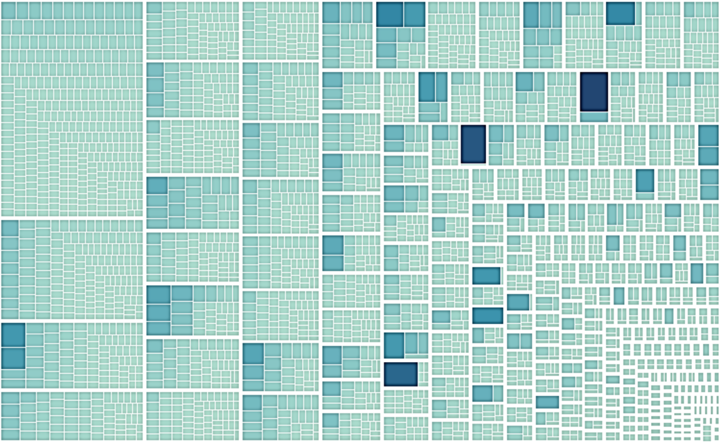
Figure 14: ActiveMap of the 532 Social media users identified as potential front-users

Figure 14 depicts the temporal activity of the above found $532$ Social media users as suspect front users, with a distance of less than $1.09$ from the DVR. The visualization includes only days in which users are active and post at least five different posts. Users are separated with thick white lines, and their days of activity are separated with internal thin white lines. Each Activemap branch of the tree denotes a user, and each leaf is a single day. The leaves show a double mapping of both size and color - days with high activity are larger and darker. Users are arranged in order of the number of active days, with users with the least active days at the bottom-right corner and users with most active days in the upper left. This visualization allows us to quickly identify that many of these users show either a larger than normal activity volume over the entire period or during specific days. Taking into account these are reviews for films, it is highly unlikely, for example, for one user to write fifty such reviews during a single day, as is the case for some.

In summary, we see that LPA can easily find suspected front-users in a social media domain.

6 Related Work

Power law distributions are prevalent in nature, and more so in empirical data (Newman, 2005). Power-law distributions were found in a wide-area of situations, among them allometric scaling in animals (West et al., 1997), number of citations received by scientific papers (Price, 1965), frequency of personal names (Zanette and Manrubia, 2001), and population of US cities as recorded in 2000 (Newman, 2005). In a power-law distribution, extreme values are more likely than they would be in a Gaussian distribution, for example. While the latter distributions are centered around a typical value, long-tail distributions do not peak at an expected value and may vary over many orders of magnitudes.

In languages, it was Zipf (1949) who demonstrated that this type of decaying relationship exists between a rank of a word and its frequency. We speak to convey meaning, and indeed, ”word meaning is a substantial determinant of frequency, and it is perhaps intuitively the best causal force in shaping frequency” (Piantadosi, 2014). In that sense, the Zipf distribution can be seen as a ’need’ distribution, related to how often we need to convey each meaning. Interestingly, popular words tend to have multiple meanings (Ferrer-i Cancho and Solé, 2003), yet they are also easier to produce (Brown and McNeill, 1966; Traxler and Gernsbacher, 2011). Zipf’s Least effort explanation relates to a lexical tradeoff between the speaker’s utility of resorting to the easy to produce, popular words and the hearer utility, which requires clarity and hence longer sentences (Zipf, 1949; Ferrer-i Cancho and Vitevitch, 2018; Hahn et al., 2020).

Vast literature supports the assumption we make here, that in each domain, there is a subset of the frequent, popular words. The Swadesh list contains universal, cultural independent available words, including ”I”, ”one”, ”many”, and ”water”, for example. An examination of frequencies of words on the lists across 17 languages found a high correlation, suggesting that these words are predictable from their meaning (Calude and Pagel, 2011). Similar findings were obtained for numbers (Piantadosi, 2014) and taboo words (Piantadosi, 2014). The same words may carry different meanings in different topics, therefore having various frequencies per various topics (Griffiths and Steyvers, 2002; Hofmann, 2013; Blei et al., 2003). Hence, our method applies within a domain where words have a specific meaning and a corresponding frequency and popularity.

In this work, we showed how LPA  creates domain-based vector representation (signature) and distance for each entity in the domain. We demonstrated that both could be used for explorations in domains and aiding in user modeling problems. Specifically, we show that it lends itself to authorship attribution and impersonation detection problems. As LPA’s entities’ attributes are slim and compact, we found it especially suitable for exploring online social media sites’ impersonations.

6.1 Social media

The prevalent anonymity within the cyber world enables unethical behaviors such as impersonation, the utilization of multiple online identities, and the spread of false information. Malicious behavior in crowdsourcing platforms is widespread and used for both fun and profit (Wang et al., 2012). The problem of online anonymity in the cyber world is addressed by employing authorship analysis and attribution techniques  (Zheng et al., 2006; Abbasi and Chen, 2008; Stein et al., 2011; Iqbal et al., 2013). For example, Barbon et al. (2017) suggest to extract baseline style features for an account and compare the style of new content in the account to determine if the account was compromised. However, social media text introduces specific challenges as it is often short, unstructured, and informal (Krippendorff, 2018).

Our primary interest is in identifying impersonations of the following types: authors that maintain multiple accounts, also termed sockpuppets (Kumar et al., 2017), and front users, a term for single accounts that are each maintained by several authors. While the latter has gained little attention, the former, i.e., detecting sockpuppets, has attracted much attention, especially from the authorship attribution community.

6.1.1 Social media authorship attribution

Authorship attribution is the science of inferring characteristics of the author from the characteristics of documents written by that author (Juola et al., 2008). Authorship attribution methods famously brought quandaries to a conclusion: they distinguished the different authors of the Federalist papers (Mosteller and Wallace, 1964) and established that the Chinese history book ’Dream of the Red Chamber’, originally thought to be written by a single author, was the product of a collaborative work (Hu et al., 2014).

Authorship analysis, rooted in stylometry, is the process of examining the characteristics of a piece of writing to conclude its authorship. Authorship identification determines the likelihood that a particular author produced a piece of writing by examining other writings by that author (Zheng et al., 2006). Until the late 1990s, authorship analysis research was dominated by attempts to define stylometry writing style features. Holmes (1998) explored the use of text length and vocabulary richness to identify a unique writing style per author. Burrows (1987) found that the 100 most frequent words can represent an author’s style.

The modern analysis methods turn to classifiers. According to a predefined feature-set, classification-based authorship attribution methods learn each author’s style and determine the author of a new text accordingly.  Narayanan et al. (2012) show that traditional classification methods for authorship analysis do not perform well over large real-world corpora of small texts. For example, Linear Discriminant Analysis does not perform well due to the data’s sparsity, while simple classifiers perform better. They further demonstrate that it is challenging to scale classification beyond a few hundred authors. However, this is the setting in ’the wild’ - large real-life corpora with a large open candidate set (Koppel et al., 2011). They further identify that the large candidate-set introduces a scalability problem. A single classifier cannot be trained to classify to $N>>1$ (10,000 authors in their case) classes, even with a small feature set. A one vs. all solution with $N$ binary classifiers is also not feasible. Instead, they repeatedly choose a fraction of the feature-set and find top matching candidates using cosine similarity. The chosen candidate, most times as a top match, is selected as the author of the anonymous text.  Koppel and Winter (2014) explore the use of similarity methods. They claim that naive similarity approaches do not work well when the text is short and the candidate set is large. Instead, they suggest to add impostors from the same domain and repeat the similarity test over a different subset of the features. The writer that scores highest on the majority of the tests is chosen as the author. Rocha et al. (2016) review authorship analysis methods for detecting online deceptions and impersonations in open source coding authorship, social networks, and social media, and discuss the limitations of classification-based methods. Current state-of-the-art works consider, among other attributes, character-grams, and used symbols such as preferred punctuation marks or emojis (Koppel et al., 2009; Schwartz et al., 2013b; Shrestha et al., 2017; Neal et al., 2018).

LPA creates, for each entity, a distance and a slim vector representation with respect to a domain, and can thus be applied to distinguish between thousands of authors. We conducted an all vs. all experiment for over 4000 authors, yielding 16 million comparisons, to detect authors of multiple social media accounts. However, while the works above considered any online text and included an extensive set of supporting features, we merely work with used text frequencies and require that all text samples relate to a specific domain. In this sense, our work is closer to Plagiarism, which measures the distance between texts to establish whether a single author has written them, but makes no attempt to identify or characterize the author (Clough, 2000; Vani and Gupta, 2018). Another field in which prominent works utilize similar methods is text categorization. Bigi (2003) used a back-off probability model to categorize texts in large corpora by measuring the KLD distance between the probability distribution of a document and the probability distribution of each category. Latent Semantic Indexing (LSI) analysis algorithm (Deerwester et al., 1990) is a document indexing method to optimize search engines. The method considers synonyms that do not appear in the text yet might appear in other texts. LSI aggregates all the synonyms under the same term with the idea of reducing dimensions in the search process. In our method, we do not aggregate synonyms, as we see the use of a specific term and not another as a signature usage.

The problem of high dimensionality in social media was also addressed by Zhang et al. (2014). They designed a framework that analyzes the text to find features and then reduces dimensions before performing the classification. They found that simple distance cosine-metric over a TFIDF vector representations of the text can attribute over 56% of the samples to the correct author. They were able to improve the result by utilizing meta-learning methods. In this work, we do not use a large set of different features to describe an author. We further showed that LPAoutperforms TFIDF in identifying authorship of multiple social-media accounts.

6.2 Temporal analysis

One of the application suggested in our work is identifying front-users, a social media account operated by multiple authors. We then corroborate our findings by looking at their online temporal activity. In the following, we give a short review of online temporal activity patterns and anomalies.

6.2.1 Normal activity patterns

Users are not expected to be consistently active. Barabási and Albert (1999) found increasing evidence that a wide range of human activities shows bursts of extensive activity, separated by long periods of inactivity. Hence, we will consider suspicious a user with a very consistent activity pattern. Ferraz Costa et al. (2015) characterized the distribution of postings inter-arrival times of users postings and find four categories of behaviors that show repetitive patterns. They suggested a Rest-Sleep-and-Comment (RSC) generative model that accommodates these categories to model users’ online behavior on social media sites. Viswanath et al. (2014) studied the behavior of black-market activity in social media networks (purchase of Facebook likes). Their study found that the granularity of a single day gave the best results. While they considered the number of likes per day, they also remarked that the same could be applied to any other user behavior. We use the number of published reviews per day as our user activity baseline for our temporal method.

6.2.2 Analytic visualization

Social media data visualization has become a conventional method to analyze and summarize information  (Schreck and Keim, 2013). Visualizations exist for information flow  (Chen et al., 2016), sentiment divergence  (Cao et al., 2015) and early flood detection  (Johnson and Shneiderman, 1991). Visual techniques are used for anomaly detection in a variety of settings: Internet security utilizing Border Gateway Protocol data  (Steiger and Schmitz, 2014), GPS data  (Kietzmann et al., 2011), Local events on Twitter and Sensor networks  (Snijders, 2001). Here, we present and employ a tree-map visualization specifically designed to highlight the characteristics we are interested in - consistency and intensity of posting periods.

7 Discussion

In this work, we have presented LPA, a method for finding latent personal signatures of entities in a domain. In a domain comprised of a collection of entities’ elements, LPA  creates two representations for each entity: its relative distance from the domain and its relative signature. The relative signature is a vector representation determining which elements most separate the entity from the domain. Created initially for text, we considered here specific textual domains, in which each entity is a text sample (a book, a chapter, or a social media user account), and the elements are the terms. We explore the different characteristics and uses of the entities’ distances and signatures for context-based authorship attribution and two types of impersonations in a social media domain: authoring different user accounts while maintaining different online personas for each, and front-users, which are accounts maintained by several authors pretending to be a single author.

We demonstrated that LPA creates signatures that are meaningful in several domains. In Section 3.4 we demonstrated the construction of LPA distances and signatures for countries Spotify songs listening habits. Countries with a smaller distance to the domain had similar listening habits to that of the domain (mostly listened to popular songs). Countries more distant from the domain tend to listen more to local music (while still listening to popular music). Two similarly distant countries may have very different listening habits, as is determined by their domain-relative signatures. To illustrate which countries have similar listening habits, we computed the distances between all countries’ signatures. Figure 15 shows the PCA computed over the resulted distance matrix. The first dimension accounts for 47.7% of the variance, and the second for 16.8%. Some of the results are intuitive. Spanish-speaking countries like Spain, Guatemala, and Mexico are closer together in the lower right corner. Paraguay and Panama are very close together while being relatively close to the Spanish cluster. On the periphery of this cluster are El Salvador, Bolivia, and Honduras. Interestingly, Cyprus and Greece are very close to Estonia, Lithuania, Latvia, and Slovakia. Another intriguing cluster in the middle left consists of Denmark, Sweden, the USA, Germany, Indonesia, Malaysia, and Hong Kong.

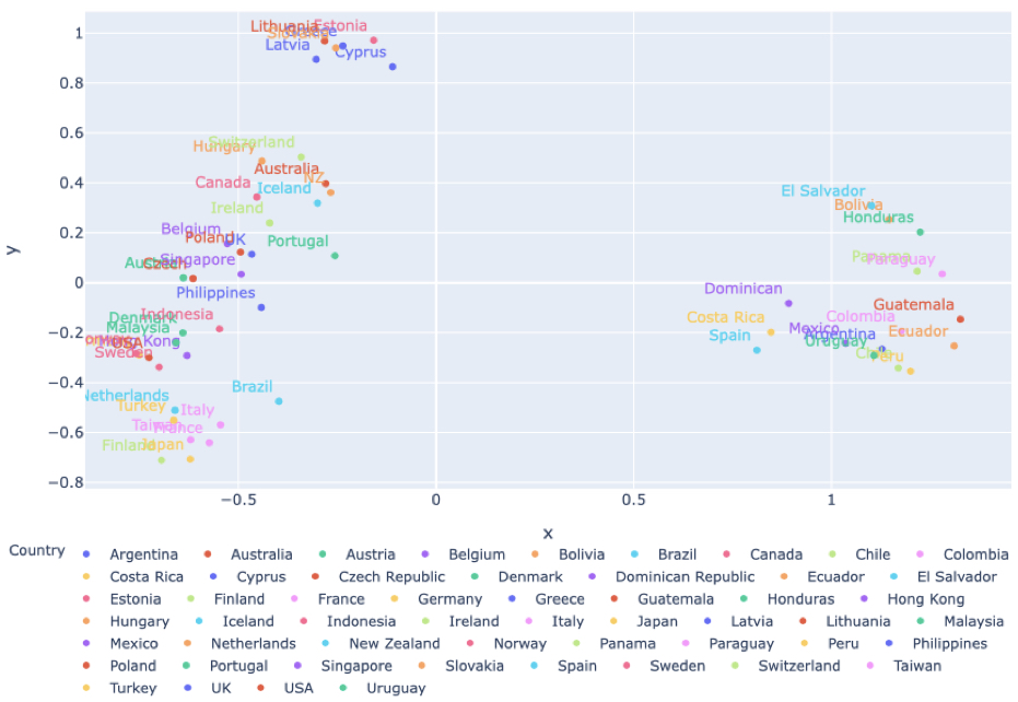
Figure 15: A PCA of the distance matrix table of Countries Spotify music LPA-signatures. The first dimension accounts for 47.7% of the variance, and the second for 16.8%.

LPA  has several limitations. As computed in Section 4.4, the sample size required to preserve a book’s chapter’s distance from a domain is of the order of the size of the average book chapter’s length. LPA also has limitations when used in social media and short text. Short-text written online contains typical typos and symbols. Therefore, the state-of-the-art methods for authorship attribution ’in the wild’ (Koppel et al., 2013) are the ones identifying these styling differences (Schwartz et al., 2013b; Shrestha et al., 2017). LPA, on the other hand, offers an unsupervised yet quick and practical method for determining vector representations for users, and is not equipped to work with unseen text. Instead, LPA-signature representations may be used as additional features in learning-based authorship attribution methods.

LPA Python code is available from Alon et al. (2021) in https://github.com/ScanLab-ossi/LPA.

8 Conclusions

We have demonstrated a method for finding how users differ in their language usage from a domain. We considered four different distance metrics for establishing this difference and, based on several defined criteria, found $\textit{KLD}_{\varepsilon}$ the best suited. Building on this finding, we devised personal signatures for users within a domain, termed LPA, and determined users’ distance from the domain. LPA  finds a domain-related distance and signature for users, or entities, in a domain. We showed that these could be used for unsupervised exploration within a domain for authorship attribution and impersonation detection. In social media, LPA can be used for identifying sockpuppets and front-user accounts. In future work, we intend to explore the use of LPA-signatures as features in learning-based attribution tasks and user modeling in recommender systems.

Declarations

Funding: The research was partially funded by the Magnet Infomedia Consortium, Israel. Conflict of interest: The authors declare that they have no conflict of interest. Availability of code, data and material: Code and data are available from http://scan.haifa.ac.il/data.

Appendix A - Distance Metrics

A distance metric $d$ on a set $X$ is a function $d:X\times X\rightarrow[0,\infty)$. I.e., it receives two elements in the set and gives the distance between them as a real, non-negative number. To be a true metric, such a function needs to fulfill the following four criteria:

•

Non-negativity: $d(x,y)\geq 0$. The distance between any two elements is greater or equal to zero.

•

symmetry: $d(x,y)=d(y,x)$. Distance is independent of starting point - for any two elements x,y in the set, the distance from x to y is the same as the distance from y to x.

•

Identity of indiscernibles: $d(x,y)=0\leftrightarrow x=y$. Two elements have a zero distance from each other if and only if they are the same element.

•

Triangle inequality: $d(x,z)\leq d(x,y)+d(y,z)$. The shortest path is a direct one - given two elements, x,z in the set, it is never shorter to go through a third one, y.

We show here that each of our selected metrics, as described in Section 3.2.1, is a distance metric by the definition given in Section Appendix A - Distance Metrics. Specifically, we show that the discussed distance metrics in  3.2.1 all satisfy the following three properties: Non negativity, Symmetry and Identity of indiscernibles.

RBD distance metric

Non negativity: We first notice that $\sum_{d=1}^{\infty}p^{d-1}$ is the sum of the geometric progression $p^{d-1}$ and is therefore equal to $\frac{1}{1-p}$. since $A_{d}\leq 1$, we get

$$\sum_{d=1}^{\infty}p^{d-1}\cdot A_{d}\leq\frac{1}{1-p}$$

and therefore

$$(1-p)\sum_{d=1}^{\infty}p^{d-1}\cdot A_{d}\leq(1-p)\frac{1}{1-p}=1$$

As $p$ is in the range $[0,1]$ and $A_{d}$ is non-negative we also get

$$(1-p)\sum_{d=1}^{\infty}p^{d-1}\cdot A_{d}\geq 0$$

Hence RBO is always in the range $[0,1]$. As $RBD=1-RBO$ it is also in that range.

Symmetry: For two lists, $V_{1},V_{2}$, $A_{d}$ is defined by the intersection of the lists over the first $d$ terms. This is a symmetrical property - the intersection of $S$ with $T$ is the same as the intersection of $T$ with $S$. $p$ is an independent parameter, and we therefore have $RBO(V_{1},V_{2},p)=RBO(V_{2},V_{1},p)$, and hence this also holds for RBD.

Identity of indiscernibles: Let us consider $V_{1}=V_{2}$, that is for every term $d$, $V_{1}(d),V_{2}(d)$. Then $\forall d,X_{d}=d$ and $A_{d}=1$. We then have

$$\sum_{d=1}^{\infty}p^{d-1}\cdot A_{d}=\sum_{d=1}^{\infty}p^{d-1}$$

As before, this is the sum of the geometric progression $p^{d-1}$ and is equal $\frac{1}{1-p}$. Therefore, for $V_{1}=V_{2}$ we get $RBO(V_{1},V_{2},p)=1$ and $RBD(V_{1},V_{2},p)=0$.
Now, consider two distinct lists. that is, for some term d, $V_{1}(d)\neq V_{2}(d)$. For that term we have $X_{d}<d$ and $A_{d}<1$. We therefore have

$$\sum_{d=1}^{\infty}p^{d-1}\cdot A_{d}<\frac{1}{1-p}$$

and therefore $RBO(V_{1},V_{2},p)<1$ and $RBD(V_{1},V_{2},p)>0$.

Cosine Similarity

As we are dealing with frequency vectors all coordinates are non negative. All vectors are therefore in the first orthant and the angles between them are in the range $[0,\pi/2]$ radians and therefore $cos\theta$ is in the range $[0,1]$ and so is $1-cos\theta$.
Symmetry: Both the dot product and the standard multiplication are commutative operations and therefore $D(V_{1},V_{2})=\frac{V_{1}\cdot V_{2}}{\|V_{1}\|\times\|V_{2}\|}=\frac{V_{2}\cdot V_{1}}{\|V_{2}\|\times\|V_{1}\|}=D(V_{2},V_{1})$, and therefore also $1-D(V_{1},V_{2})=1-D(V_{2},V_{1})$.
Identity of Indiscernibles: First, we note that for vectors of length n, the standard dot product $V_{1}\cdot V_{2}$ is defined as $\sum_{i=1}^{n}V_{1_{i}}\times V_{2_{i}}$ and the standard euclidean norm is defined as $\sqrt{\sum_{i=1}^{n}(V_{i})^{2}}$. Assume $V_{1}=V_{2}$, i.e. for every i $V_{1}(i)=V_{2}(i)$. We then have $V_{1}\cdot V_{2}=\sum_{i=1}^{n}V_{1}(i)\times V_{2}(i)=\sum_{i=1}^{n}V_{1}(i)\times V_{1}(i)=\sum_{i=1}^{n}V_{1}(i)^{2}$. We also have $\|V_{1}\|=\|V_{2}\|$ and therefore $\|V_{1}\|\times\|V_{2}\|=\|V_{1}\|^{2}=\sqrt{\sum_{i=1}^{n}V_{1}(i)^{2}}^{2}=\sum_{i=1}^{n}V_{1}(i)^{2}$. Therefore for $V_{1}=V_{2}$ we have $D(V_{1},V_{2})=\frac{V_{1}\cdot V_{2}}{\|V_{1}\|\times\|V_{2}\|}=\frac{\sum_{i=1}^{n}V_{1}(i)^{2}}{\sum_{i=1}^{n}V_{1}(i)^{2}}=1$ and $1-D(V_{1},V_{2})=0$.

Assume $1-D(V_{1},V_{2})=0$, that is $D(V_{1},V_{2})=1$. As we’ve seen when proving non-negativity, this implies that the angle $\theta$ between $V_{1}$ and $V_{2}$ is zero. Since both vectors are frequency vectors, i.e. $\|V_{1}\|=\|V_{2}\|=1$ this means they are the same vector.

L1 Norm

Non negativity: It’s enough to prove non negativity for each element of the sum, but that is assured by the absolute value.
Symmetry: Again, it’s enough to show symmetry for each element of the sum. We note that $(V_{1}(x)-V_{2}(x))=-(V_{2}(x)-V_{1}(x))$ and therefore $\arrowvert(V_{1}(x)-V_{2}(x))\arrowvert=\arrowvert(V_{2}(x)-V_{1}(x))\arrowvert$
Identity of indiscernibles: Assume $V_{1}=V_{2}$, i.e for every $x\in X$ we have $V_{1}(x)=V_{2}(x)$. Then $V_{1}(x)-V_{2}(x)=0$ and we have $L1(V_{1},V_{2})=0$.
Assume $V_{1}\neq V_{2}$ i.e. for some $x\in X$ we have $V_{1}(x)\neq V_{2}(x)$. For that $x$ we have $\big{[}V_{1}(x)-V_{2}(x)\big{]}>0$ and as all elements in the sum are non negative we have $L1(V_{1},V_{2})>0$.

KL divergence

Non negativity: It is enough to show that each element in the sum is non negative. For every $x\in X$ either $V_{1}(x)<V_{2}(x)$, $V_{1}(x)V_{2}(x)$ or $V_{1}(x)=V_{2}(x)$. If $V_{1}(x)<V_{2}(x)$ then $V_{1}(x)-V_{2}(x)<0$ and $log\frac{V_{1}(x)}{V_{2}(x)}<0$. Therefore $\big{[}V_{1}(x)-V_{2}(x)\big{]}log\frac{V_{1}(x)}{V_{2}(x)}>0$. If $V_{1}(x)>V_{2}(x)$ then $V_{1}(x)-V_{2}(x)>0$ and $log\frac{V_{1}(x)}{V_{2}(x)}>0$ and again $\big{[}V_{1}(x)-V_{2}(x)\big{]}log\frac{V_{1}(x)}{V_{2}(x)}>0$. Lastly, if $V_{1}(x)=V_{2}(x)$ then $V_{1}(x)-V_{2}(x)=0$ and $log\frac{V_{1}(x)}{V_{2}(x)}=0$ and we have $\big{[}V_{1}(x)-V_{2}(x)\big{]}log\frac{V_{1}(x)}{V_{2}(x)}=0$
Symmetry: We note that $(V_{1}(x)-V_{2}(x))=-(V_{2}(x)-V_{1}(x))$ and likewise $log\frac{V_{1}(x)}{V_{2}(x)}=-log\frac{V_{2}(x)}{V_{1}(x)}$ and therefore $(V_{1}(x)-V_{2}(x))log\frac{V_{1}(x)}{V_{2}(x)}=(V_{2}(x)-V_{1}(x))log\frac{V_{2}(x)}{V_{1}(x)}$. Again, this is true for each element in the sum and therefore holds for the entire sum.
Identity of indiscernibles: Assume $V_{1}=V_{2}$, i.e for every $x\in X$ we have $V_{1}(x)=V_{2}(x)$. Then $V_{1}(x)-V_{2}(x)=0$ and $log\frac{V_{1}(x)}{V_{2}(x)}=1$ and we have $\big{[}V_{1}(x)-V_{2}(x)\big{]}log\frac{V_{1}(x)}{V_{2}(x)}=0$.
Assume $V_{1}\neq V_{2}$ i.e. for some $x\in X$ we have $V_{1}(x)\neq V_{2}(x)$. For that $x$ we have $\big{[}V_{1}(x)-V_{2}(x)\big{]}log\frac{V_{1}(x)}{V_{2}(x)}>0$ and as all elements in the sum are non negative we have $D([V_{1}\Arrowvert V_{2}]=\sum_{x\in X}\Bigg{[}\big{[}V_{1}(x)-V_{2}(x)\big{]}log\Big{[}\frac{V_{1}(x)}{V_{2}(x)}\Big{]}\Bigg{]}>0$

Appendix A Datasets details

Books dataset:

The Books dataset is comprised of 30 English language books, taken from the Gutenberg project’s most popular books list. Each book is divided into chapters, varying from 7 to 61 chapters per book. We included only chapters that contain more than 150 words in the text and omitted words that appear less than five times in the book to avoid the extreme consequences of a very long tail. Each text snippet is labeled with an author’s name, and belongs to a book, and more specifically to a chapter in the book. In the Validation section, we use this subdivision to validate whether our method is able to distinguish between two texts written by the same person and two texts written by different people. We also test its ability to distinguish between a text written by one person and a text written by several, by collecting a number of chapters from different books to one virtual book. Table 8in Appendix A lists the book names and relevant statistics.

IMDb reviews dataset:

IMDb (Internet Movie Database) is among the world’s most popular and authoritative sources for movie, TV and celebrity content. It offers a searchable database of more than 185 million data items, including more than 3.5 million films. This dataset contains 1,406,000 movie reviews, spanning the period of July 1998 - June 2016. We use their movie reviews text as our dataset for demonstrating the applications of our method. We define a user/author (contributor) as a registered person who published a movie review on IMDb. Each author is identified by a unique user id and alias. Each review contains a text, a timestamp, and an author ID. The original obtained IMDb dataset contained $467,961$ users. To have a large enough sample of text for each user, we extracted only users who published at least 30 reviews. 3,969 users met this criterion. We defined $n=30$ (number of different reviews per user) as our lower threshold to achieve statistical inference. The choice of $n=30$ for a boundary between small and large samples is already used as a rule of thumb in many research areas: ”The number 30 seems to have arisen from the understanding that with fewer than 30 cases, you were dealing with small samples that required specialized handling with small-sample statistics instead of the critical-ratio approach we have been taught” (Cohen, 1990).

Table 8: Books datasets characteristics

#	Book Name	Unique	Chapters
		Terms	(Avergae)
1	A Study in Scarlet , Doyle, Arthur Conan	16,388	14
2	A Tale of Two Cities , Dickens, Charles	51,519	39
3	Adventures of Huckleberry Finn ,Twain, Mark	39,066	43
4	Alice’s Adventures in Wonderland , Carroll, Lewis	9,066	12
5	Anne of Green Gables,Montgomery, L. M. (Lucy Maud)	41,005	38
6	Emma , Austen, Jane	57,185	55
7	Great Expectations ,Dickens, Charles	68,069	59
8	Grey Town ,Baldwin ,Gerald	22,934	24
9	Gulliver Of Mars ,Arnold ,Edwin	25,898	27
10	Gulliver’s Travels, Swift, Jonathan	39,117	39
11	Jane Eyre: An Autobiography ,Bront$\ddot{e}$, Charlotte	76,612	39
12	Little Women ,Alcott, Louisa May	73,266	47
13	Notes from the underground, Dostoevsky, Fyodor	13,501	14
14	Oliver Twist ,Dickens, Charles	61,895	53
15	Peter Pan ,Barrie, J. M. (James Matthew)	17,095	17
16	Poll (The Lively), Ballantyne, R.M.	12,240	13
17	Pride and Prejudice, Austen, Jane	43,722	61
18	Sense and Sensibility, Austen, Jane	42,478	50
19	The Adventures of Sherlock Holmes, Doyle, Arthur Conan	34,559	7
20	The Adventures of Tom Sawyer , Twain, Mark	27,077	35
21	The Devil-Tree of El Dorado, Aubrey, Frank	39,409	40
22	The Following of the Star, Barclay ,Florence	31,335	32
23	The King in Yellow, Chambers, Robert W. (Robert William)	30,425	28
24	The Life and Adventures of Robinson Crusoe, Defoe, Daniel	41,598	20
25	The Picture of Dorian Gray ,Wilde, Oscar	29,947	20
26	The Time Machine ,Wells, H. G. (Herbert George)	13,068	12
27	The Souls of Black Folk, DuBois, W.E.Burghardt	27,046	29
28	Treasure Island ,Stevenson, Robert Louis	25,451	32
29	Wuthering Heights ,Bront$\ddot{e}$, Emily	47,183	34
30	Frey and His Wife, Hewlett, Maurice Henry	9278	10
Total		1,067,432	943

Table 9: IMDb dataset characteristics

IMDb dataset property	Value
Start date	July 1998
End date	June 2016
Number of unique movies	7,696
Users with more than 30 reviews	3,969
Reviews	474,961
Unique Nouns	273,025
Avg unique nouns per user	2,925
Avg number of reviews per movie	61.7
Stdev number of reviews per movie	71
Avg number of reviews per author	119.6
Stdev number of reviews per author	205

References

- Abbasi and Chen (2008) Abbasi A, Chen H (2008) Writeprints: A stylometric approach to identity-level identification and similarity detection in cyberspace. ACM Transactions on Information Systems (TOIS) 26(2)
- Akmajian et al. (2017) Akmajian A, Farmer AK, Bickmore L, Demers RA, Harnish RM (2017) Linguistics: An introduction to language and communication. MIT press
- Alon et al. (2021) Alon U, Mokryn O, Hershberg U (2021) Using domain based latent personal analysis of b cell clone diversity patterns to identify novel relationships between the b cell clone populations in different tissues. Frontiers in immunology 12
- Argamon et al. (2009) Argamon S, Koppel M, Pennebaker JW, Schler J (2009) Automatically profiling the author of an anonymous text. Commun ACM 52(2):119–123
- Baker and McCallum (1998) Baker LD, McCallum AK (1998) Distributional clustering of words for text classification. In: Proceedings of the 21st annual international ACM SIGIR conference on Research and development in information retrieval, pp 96–103
- Barabasi (2005) Barabasi AL (2005) The origin of bursts and heavy tails in human dynamics. Nature 435(7039):207
- Barabási and Albert (1999) Barabási AL, Albert R (1999) Emergence of scaling in random networks. SCIENCE 286:509 – 512
- Barbon et al. (2017) Barbon S, Igawa RA, Zarpelão BB (2017) Authorship verification applied to detection of compromised accounts on online social networks. Multimedia Tools and Applications 76(3):3213–3233
- Ben-Shoshan and Mokryn (2018) Ben-Shoshan H, Mokryn O (2018) Activemap: Visual analysis of temporal activity in social media sites. In: Proceedings of the 23rd International Conference on Intelligent User Interfaces Companion, pp 1–2
- Ben-Tovim (2008) Ben-Tovim R (2008) Robinson crusoe, wittgenstein, and the return to society. Philosophy and Literature 32(2):278–292
- Bigi (2003) Bigi B (2003) Using kullback-leibler distance for text categorization. In: European Conference on Information Retrieval, Springer, pp 305–319
- Blei et al. (2003) Blei DM, Ng AY, Jordan MI (2003) Latent dirichlet allocation. Journal of machine Learning research 3(Jan):993–1022
- Brinegar (1963) Brinegar CS (1963) Mark twain and the quintus curtius snodgrass letters: A statistical test of authorship. Journal of the American statistical Association 58(301):85–96
- Brown and McNeill (1966) Brown R, McNeill D (1966) The “tip of the tongue” phenomenon. Journal of verbal learning and verbal behavior 5(4):325–337
- Burrows (1987) Burrows JF (1987) Word-patterns and story-shapes: The statistical analysis of narrative style. Literary and Linguistic Computing 2(2):61–70
- Calude and Pagel (2011) Calude AS, Pagel M (2011) How do we use language? shared patterns in the frequency of word use across 17 world languages. Philosophical Transactions of the Royal Society B: Biological Sciences 366(1567):1101–1107
- Ferrer-i Cancho and Solé (2003) Ferrer-i Cancho R, Solé RV (2003) Least effort and the origins of scaling in human language. Proceedings of the National Academy of Sciences 100(3):788–791
- Ferrer-i Cancho and Vitevitch (2018) Ferrer-i Cancho R, Vitevitch MS (2018) The origins of zipf’s meaning-frequency law. Journal of the Association for Information Science and Technology 69(11):1369–1379
- Cao et al. (2015) Cao N, Lu L, Lin YR, Wang F, Wen Z (2015) Socialhelix: visual analysis of sentiment divergence in social media. Journal of Visualization 18(2):221–235
- Chen et al. (2016) Chen S, Chen S, Wang Z, Liang J, Yuan X, Cao N, Wu Y (2016) D-map: Visual analysis of ego-centric information diffusion patterns in social media. In: Visual Analytics Science and Technology (VAST), 2016 IEEE Conference on, IEEE, pp 41–50
- Clough (2000) Clough P (2000) Plagiarism in natural and programming languages: an overview of current tools and technologies. Citeseer
- Cohen (1990) Cohen J (1990) Things i have learned (so far). American psychologist 45(12):1304
- Deerwester et al. (1990) Deerwester S, Dumais ST, Furnas GW, Landauer TK, Harshman R (1990) Indexing by latent semantic analysis. Journal of the American society for information science 41(6):391–407
- Dumais (2004) Dumais ST (2004) Latent semantic analysis. Annual review of information science and technology 38(1):188–230
- Ferrara et al. (2016) Ferrara E, Varol O, Davis C, Menczer F, Flammini A (2016) The rise of social bots. Communications of the ACM 59(7):96–104
- Ferraz Costa et al. (2015) Ferraz Costa A, Yamaguchi Y, Juci Machado Traina A, Traina Jr C, Faloutsos C (2015) Rsc: Mining and modeling temporal activity in social media. In: Proceedings of the 21th ACM SIGKDD International Conference on Knowledge Discovery and Data Mining, ACM, pp 269–278
- Freud (1925) Freud S (1925) Negation. International Journal of Psycho-Analysis 6:367–371
- Griffiths and Steyvers (2002) Griffiths TL, Steyvers M (2002) A probabilistic approach to semantic representation. In: Proceedings of the annual meeting of the cognitive science society, vol 24
- Hahn et al. (2020) Hahn M, Jurafsky D, Futrell R (2020) Universals of word order reflect optimization of grammars for efficient communication. Proceedings of the National Academy of Sciences 117(5):2347–2353
- Hofmann (2013) Hofmann T (2013) Probabilistic latent semantic analysis. arXiv preprint arXiv:13016705
- Holmes (1998) Holmes DI (1998) The Evolution of Stylometry in Humanities Scholarship. Literary and Linguistic Computing 13(3):111 –117
- Hu et al. (2014) Hu X, Wang Y, Wu Q (2014) Multiple authors detection: a quantitative analysis of dream of the red chamber. Advances in Adaptive Data Analysis 6(04):1450012
- Iqbal et al. (2013) Iqbal F, Binsalleeh H, Fung BC, Debbabi M (2013) A unified data mining solution for authorship analysis in anonymous textual communications. Information Sciences 231:98–112
- Johnson and Shneiderman (1991) Johnson B, Shneiderman B (1991) Tree-maps: A space-filling approach to the visualization of hierarchical information structures. In: Proceedings of the 2nd conference on Visualization’91, IEEE Computer Society Press, pp 284–291
- Juola et al. (2008) Juola P, et al. (2008) Authorship attribution. Foundations and Trends® in Information Retrieval 1(3):233–334
- Kaplan and Haenlein (2010) Kaplan AM, Haenlein M (2010) Users of the world, unite! the challenges and opportunities of social media. Business horizons 53(1):59–68
- Kietzmann et al. (2011) Kietzmann JH, Hermkens K, McCarthy IP, Silvestre BS (2011) Social media? get serious! understanding the functional building blocks of social media. Business horizons 54(3):241–251
- Kilgarriff and Rose (1998) Kilgarriff A, Rose T (1998) Measures for corpus similarity and homogeneity. In: Proceedings of the Third Conference on Empirical Methods for Natural Language Processing, pp 46–52
- Koppel and Winter (2014) Koppel M, Winter Y (2014) Determining if two documents are written by the same author. Journal of the Association for Information Science and Technology 65(1):178–187
- Koppel et al. (2009) Koppel M, Schler J, Argamon S (2009) Computational methods in authorship attribution. Journal of the American Society for information Science and Technology 60(1):9–26
- Koppel et al. (2011) Koppel M, Schler J, Argamon S (2011) Authorship attribution in the wild. Language Resources and Evaluation 45(1):83–94
- Koppel et al. (2013) Koppel M, Schler J, Argamon S (2013) Authorship Attribution: What’s Easy and What’s Hard? The Journal of Law, Economics & Policy 39(2006):317–331
- Krippendorff (2018) Krippendorff K (2018) Content analysis: An introduction to its methodology. Sage publications
- Kullback and Leibler (1951) Kullback S, Leibler RA (1951) On Information and Sufficiency. The Annals of Mathematical Statistics 22(1):79–86
- Kumar et al. (2017) Kumar S, Cheng J, Leskovec J, Subrahmanian V (2017) An army of me: Sockpuppets in online discussion communities. In: Proceedings of the 26th International Conference on World Wide Web, pp 857–866
- Mosteller and Wallace (1964) Mosteller F, Wallace DL (1964) Inference and disputed authorship: The Federalist
- Narayanan et al. (2012) Narayanan A, Paskov H, Gong NZ, Bethencourt J, Stefanov E, Shin ECR, Song D (2012) On the feasibility of internet-scale author identification. In: 2012 IEEE Symposium on Security and Privacy, IEEE, pp 300–314
- Neal et al. (2018) Neal T, Sundararajan K, Fatima A, Yan Y, Xiang Y, Woodard D (2018) Surveying stylometry techniques and applications. ACM Computing Surveys (CSUR) 50(6):86
- Newman (2005) Newman ME (2005) Power laws, pareto distributions and zipf’s law. Contemporary physics 46(5):323–351
- Ntoulas et al. (2006) Ntoulas A, Najork M, Manasse M, Fetterly D (2006) Detecting spam web pages through content analysis. In: Proceedings of the 15th international conference on World Wide Web, ACM, pp 83–92
- Piantadosi (2014) Piantadosi ST (2014) Zipf’s word frequency law in natural language: A critical review and future directions. Psychonomic bulletin & review 21(5):1112–1130
- Price (1965) Price DJDS (1965) Networks of scientific papers. Science pp 510–515
- Rocha et al. (2016) Rocha A, Scheirer WJ, Forstall CW, Cavalcante T, Theophilo A, Shen B, Carvalho AR, Stamatatos E (2016) Authorship attribution for social media forensics. IEEE Transactions on Information Forensics and Security 12(1):5–33
- Schreck and Keim (2013) Schreck T, Keim D (2013) Visual analysis of social media data. Computer 46(5):68–75
- Schwartz et al. (2013a) Schwartz HA, Eichstaedt JC, Kern ML, Dziurzynski L, Ramones SM, Agrawal M, Shah A, Kosinski M, Stillwell D, Seligman ME, et al. (2013a) Personality, gender, and age in the language of social media: The open-vocabulary approach. PloS one 8(9)
- Schwartz et al. (2013b) Schwartz R, Tsur O, Rappoport A, Koppel M (2013b) Authorship attribution of micro-messages. In: Proceedings of the 2013 Conference on Empirical Methods in Natural Language Processing, pp 1880–1891
- Shrestha et al. (2017) Shrestha P, Sierra S, González FA, Montes M, Rosso P, Solorio T (2017) Convolutional neural networks for authorship attribution of short texts. In: Proceedings of the 15th Conference of the European Chapter of the Association for Computational Linguistics: Volume 2, Short Papers, pp 669–674
- Snijders (2001) Snijders TA (2001) The statistical evaluation of social network dynamics. Sociological methodology 31(1):361–395
- Steiger and Schmitz (2014) Steiger B, Schmitz R (2014) Computer implemented methods for visualizing correlations between blood glucose data and events and apparatuses thereof. US Patent App. 13/603,853
- Stein et al. (2011) Stein B, Lipka N, Prettenhofer P (2011) Intrinsic plagiarism analysis. Language Resources and Evaluation 45(1):63–82
- Traxler and Gernsbacher (2011) Traxler M, Gernsbacher MA (2011) Handbook of psycholinguistics. Elsevier
- Van Dijck (2009) Van Dijck J (2009) Users like you? theorizing agency in user-generated content. Media, culture & society 31(1):41–58
- Vani and Gupta (2018) Vani K, Gupta D (2018) Unmasking text plagiarism using syntactic-semantic based natural language processing techniques: Comparisons, analysis and challenges. Information Processing & Management 54(3):408–432
- Viswanath et al. (2014) Viswanath B, Bashir MA, Crovella M, Guha S, Gummadi KP, Krishnamurthy B, Mislove A (2014) Towards detecting anomalous user behavior in online social networks. In: 23rd Usenix Security Symposium, pp 223–238
- Vosoughi et al. (2018) Vosoughi S, Roy D, Aral S (2018) The spread of true and false news online. Science 359(6380):1146–1151
- Wang et al. (2012) Wang G, Wilson C, Zhao X, Zhu Y, Mohanlal M, Zheng H, Zhao BY (2012) Serf and turf: crowdturfing for fun and profit. In: Proceedings of the 21st international conference on World Wide Web, ACM, pp 679–688
- Webber et al. (2010) Webber W, Moffat A, Zobel J (2010) A similarity measure for indefinite rankings. ACM Transactions on Information Systems
- West et al. (1997) West GB, Brown JH, Enquist BJ (1997) A general model for the origin of allometric scaling laws in biology. Science 276(5309):122–126
- Zanette and Manrubia (2001) Zanette DH, Manrubia SC (2001) Vertical transmission of culture and the distribution of family names. Physica A: Statistical Mechanics and its Applications 295(1-2):1–8
- Zhang et al. (2014) Zhang C, Wu X, Niu Z, Ding W (2014) Authorship identification from unstructured texts. Knowledge-Based Systems 66:99–111
- Zheng et al. (2006) Zheng R, Li J, Chen H, Huang Z (2006) A framework for authorship identification of online messages: Writing-style features and classification techniques. Journal of the American society for information science and technology 57(3):378–393
- Zipf (1949) Zipf G (1949) Human behavior and the principle of least effort. Addison Wesley, Cambridge, Massachusetts