Graphical outputs and Spatial Cross-validation for the R-INLA package using INLAutils

Abstract

Statistical analyses proceed by an iterative process of model fitting and checking. The R-INLA package facilitates this iteration by fitting many Bayesian models much faster than alternative MCMC approaches. As the interpretation of results and model objects from Bayesian analyses can be complex, the R package INLAutils provides users with easily accessible, clear and customisable graphical summaries of model outputs from R-INLA. Furthermore, it offers a function for performing and visualizing the results of a spatial leave-one-out cross-validation (SLOOCV) approach that can be applied to compare the predictive performance of multiple spatial models. In this paper, we describe and illustrate the use of (1) graphical summary plotting functions and (2) the SLOOCV approach. We conclude the paper by identifying the limits of our approach and discuss future potential improvements.

Introduction

From its inception in 2009, the R (R Core Team, 2016) package R-INLA (Rue et al., 2009; Martins et al., 2013) has provided a convenient framework to fit latent Gaussian models within a Bayesian framework using R commands. Latent Gaussian models represent a wide and flexible class of models that includes mixed effects models and spatial and spatio-temporal models that can be applied to areal, geostatistical, and point process data. For models with a continuous spatial component, the approach combines the integrated nested Laplace approximation (INLA) (Rue et al., 2009) with the stochastic partial differential equation approach (SPDE) developed by Lindgren et al. (2011). The INLA/SPDE approach represents a computationally efficient alternative to Markov Chain Monte Carlo (MCMC) (Lindgren, 2015). Despite MCMC’s high flexibility on both data and model types, estimating the posterior distribution for the parameters remains computationally expensive in this framework. The superior computational performance of INLA/SPDE allows fitting a broad range of models applied to large data and running systematic cross-validation processes which would require considerably more time with MCMC algorithms.

Users who are not familiar with the usage of this statistical software might face difficulties in extracting and visualizing summary characteristics of the model outputs generated by R-INLA. Outputs from R-INLA consist of large nested lists, whose elements can be difficult to be identified. As a fundamental part of iterative model building, it is important for summaries and visualisations of models to be as easily accessible as possible (Gabry et al., 2019). In addition, cross-validation of spatial models as currently implemented in R-INLA does not account for spatial autocorrelation in the data. Predictions made geographically far away from the data will be less good than predictions made near the data as they rely solely on covariates without any contribution from the spatial random field. Spatial leave-one-out cross-validation is one solution to this problem where data near the hold-out data point is also removed. Here we present functions from the package INLAutils that provides functions for streamlining these aspects of the Bayesian modelling process with R-INLA.

Section 0.4 illustrates the use of commands to generate graphical summaries of R-INLA model outputs. Section 0.5 illustrates the command used to perform and visualize the results of a SLOOCV procedure applied to multiple models. In Section 0.6 we discuss the limits of the package capabilities and identify potential future improvements.

Installation

Due to technical issues with building the C binaries needed by R-INLA, the package is not available from CRAN. It can be installed the following command

install.packages("INLA",                 repos = c(getOption("repos"),                           INLA = "https://inla.r-inla-download.org/R/stable"),                 dep = TRUE)In turn, this means INLAutils is not on CRAN. It is available from www.github.com/timcdlucas/INLAutils or can be installed with the following command.

devtools::install_github(’timcdlucas/INLAutils’)

Example data analysis

To illustrate the various aspects of this package we will use the Meuse dataset (Rikken and Van Rijn, 1993) that is available in the sp package (Pebesma and Bivand, 2005). This dataset contains 155 observations of concentrations of four heavy metals. We fit a latent Gaussian regression model modform on a normal response (cadmium concentration), which includes an intercept, y.intercept, three covariates (elev, dist, om), a spatial component, f(spatial.field, model = spde), and an unstructured Gaussian error term (not displayed in the formula). In R-INLA, the spatial component is represented by a Gaussian Markov Random Field, with a Matérn covariance function. The flexibility of the the Gaussian Markov Random Field is controlled by two hyperparameters, $\theta_{1}$ and $\theta_{2}$. For comparison purposes, we fit the same model without the spatial component, modform2. We show below the data preparation and code used to run the models. Further details on coding spatial models with R-INLA can be found in Blangiardo and Cameletti (2015).

require(INLAutils)require(INLA)require(sp)data(meuse)# Define the modelsmodform <- cadmium ~ -1 + y.intercept + elev + dist + om +             f(spatial.field, model = spde)modform2 <- cadmium ~ -1 + y.intercept + elev + dist + om# Scale the spatial coordinates to make mesh construction easiercoords <- scale(meuse[, c(’x’, ’y’)])colnames(coords) <- c(’long’, ’lat’)dataf1 <- sp::SpatialPointsDataFrame(coords = coords, data = meuse[, -c(1:2)])mesh <- inla.mesh.2d(loc = sp::coordinates(dataf1),                     max.edge = c(0.2, 0.5), cutoff = 0.1)spde <- inla.spde2.matern(mesh, alpha=2) # SPDE model is definedA <- inla.spde.make.A(mesh, loc = sp::coordinates(dataf1)) # projector matrixdataframe <- data.frame(dataf1) # get dataframe with response and covariate# make index for spatial fields.index <- inla.spde.make.index(name="spatial.field",n.spde=spde$n.spde)# Prepare the datastk <- inla.stack(data=list(cadmium=dataframe$cadmium),                      A=list(A,1),                      effects=list(c(s.index,list(y.intercept=1)),                                   list(dataframe[, 5:7])),                      tag=’est’)out <- inla(modform, family = ’normal’,            data = inla.stack.data(stk, spde = spde),            control.predictor = list(A = inla.stack.A(stk), link = 1),            control.compute = list(config = TRUE),            control.inla = list(int.strategy = ’eb’))

Graphical Summaries with the autoplot, ggplot_inla_residuals and
ggplot_projection_shapefile functions

The autoplot.inla command

We provide methods for the autoplot command from ggplot2 for R-INLA models and meshes. Using ggplot2 means all visual aspects can be easily fine-tuned. The autoplot.inla method allows the user to visualize outputs from any R-INLA object (Figure 1). The command reimplements much of the functionality from the R-INLA plot command but uses ggplot2 as the plotting backend. By default the function plots provides a visual overview of (top-left): the marginal posterior distributions, prior distributions and credible intervals of the intercept (y.intercept) and coefficients for the covariates (elev, dist, om); (top-right): the marginal posterior distributions and credible intervals of model hyperparameters; the marginal posterior mean and 95% credible intervals of any random effects if specified in the model and; (bottom-left) and the linear predictor and fitted values (bottom-right). As the link function is the identity function the linear predictor and fitted values are the same in this case. These subplots can be activated or deactivated with the which argument. This function returns a list of ggplot2 plots which can be plotted together using plot_grid from the cowplot package (Wilke, 2019). The command can be used with any R-INLA model object though subplots that plot random effects are only created for models with random effects. Which subplots to create can be selected with the which argument. The other arguments to the command are priors which determines whether the priors of the fixed effects are plotted and CI which determines whether 95% credible intervals are plotted for both the fixed effects and hyperparameters.

p <- autoplot(out)cowplot::plot_grid(plotlist = p)

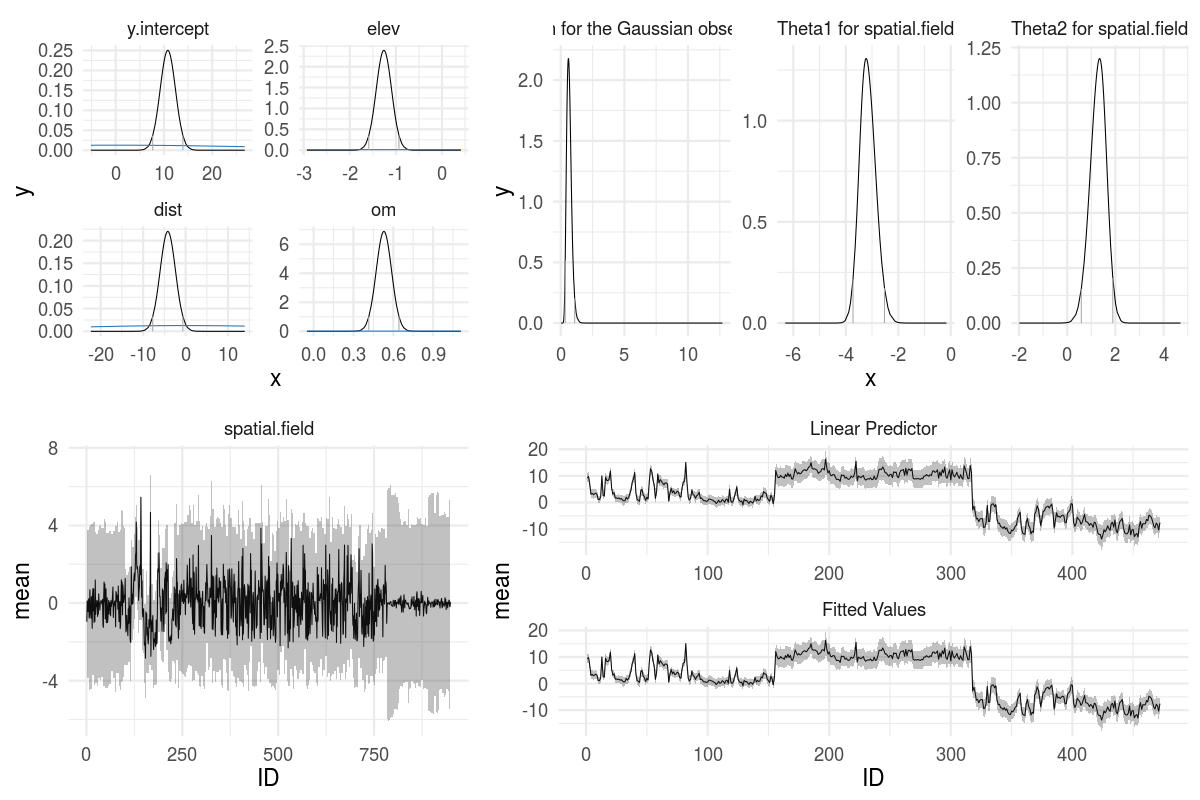
Figure 1: (four plots top-left) Marginal posterior distributions (black lines), prior distributions (blue lines) and 95% credible interval (grey vertical lines) of y.intercept and covariate coefficients for elev, dist and om. (three plots top-right) Marginal posterior distributions (black lines) and 95% credible interval (grey vertical lines) of the precision of the Gaussian unstructured error term and two hyperparameters for the spatial random field. (bottom-left) Marginal posterior mean and 95% credible intervals of the spatial random effects. (two plots bottom-right) Marginal posterior mean and 95% credible intervals of the linear predictor, and fitted values.

In the following example (Figure 2), we use ggplot2 to modify the plot of the the posterior distributions of the intercept and coefficients for the covariates, by selecting the first object of the autoplot output, with the command p[[1]]. The size and colour of the lines are modified using the ggplot2 syntax with a convenient colour palette (Lucas, 2016).

require(ggplot2)require(palettetown) # a convenient palettep[[1]] +  geom_line(aes(colour = var), size = 1.3) +  palettetown::scale_colour_poke(pokemon = ’Charmander’, spread = 4)

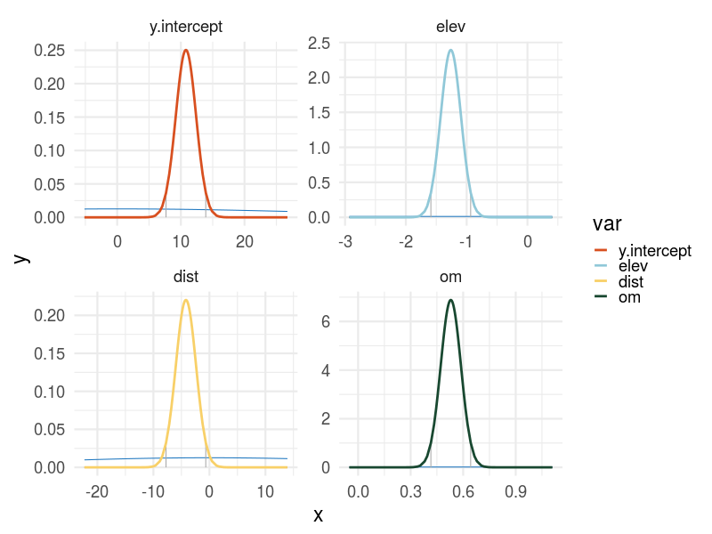
Figure 2: Visualization of the posterior distribution of the intercept (y.intercept) and covariates’ coefficients using thick lines with four distinct colours: y.intercept (red), elev (light blue), dist (orange), and om (green). The prior distributions (blue lines) and 95% credible intervals (grey vertical lines) are also shown.

The ggplot_inla_residuals command

Other important summary characteristics of R-INLA outputs can be visualized. Here, the ggplot_inla_residuals command is applied to the results of the R-INLA outputs and the response data, extracted from the meuse object, as illustrated below:

ggplot_inla_residuals(out, meuse$cadmium, binwidth = 0.1)

This function plots an histogram of the posterior probability of a replicate of each observation (Figure 3 left). The binwidth can be controlled with the argument binwidth. If the model is well calibrated (i.e. if the uncertainty estimates are accurate) the posterior probabilities are expected to be uniformly distributed (and therefore the height of the bins should be similar). In the example, the humped distribution suggests that the model is underconfident in its predictions. Figure 3 (right) illustrates the relationship between the observed (x-axis) and the predicted (y-axis) values. Values above and below the line (identity function: $y=x$) correspond to overestimation and underestimation of the data by the model, respectively. The two plots are returned as a list of ggplot objects.

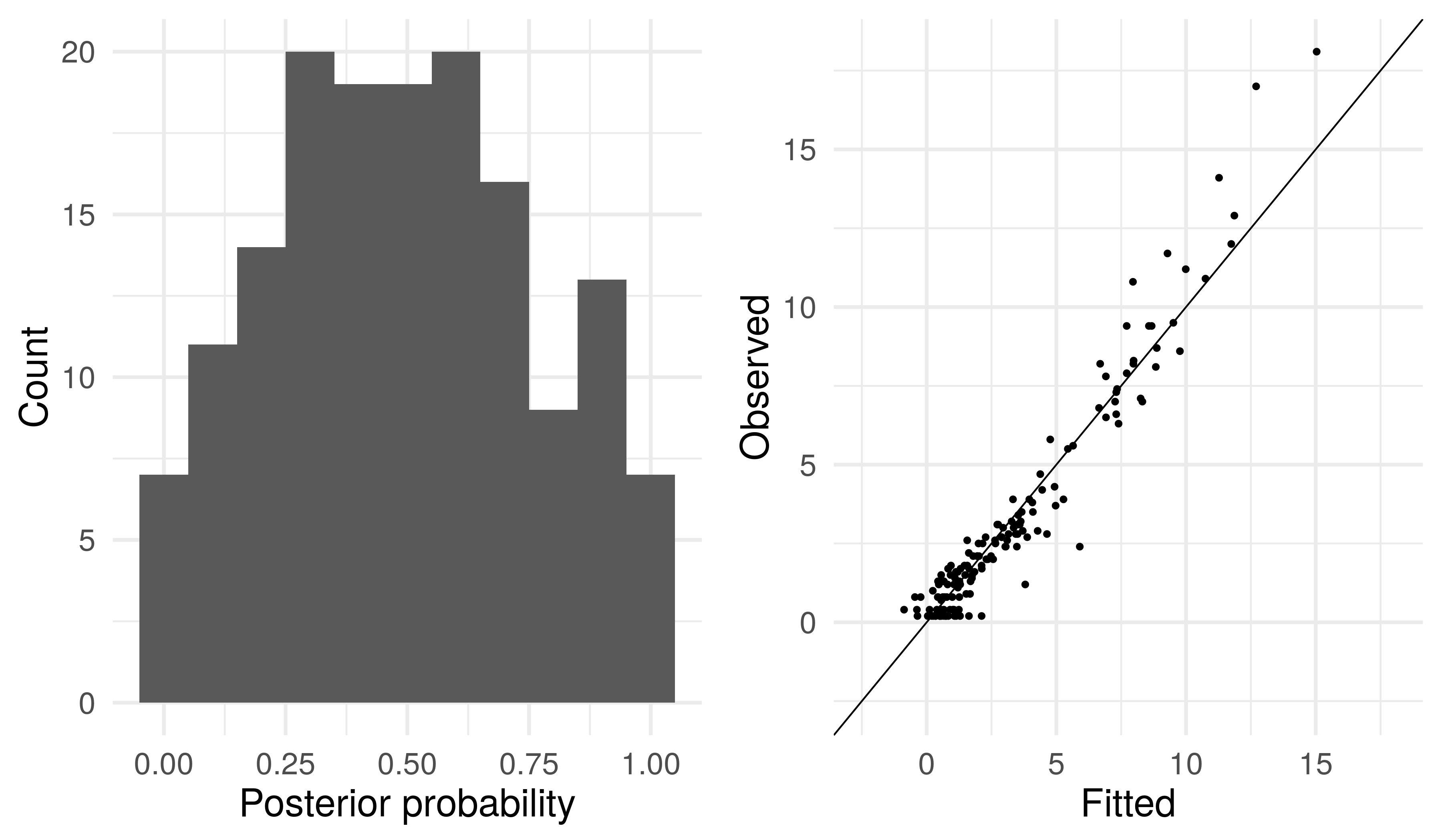
Figure 3: (Left): histogram of the posterior probability of a replicate of each observation, and (right): relationship between the observed (x-axis) and the predicted (y-axis) values. The identity function $y=x$ is illustrated by the black line.

The autoplot.inla.mesh command

For continuous-space models in R-INLA, users need to define a mesh on top of which the stochastic partial differential equation (SPDE) is built (see Lindgren (2015) for further details). In a two-dimensional spatial model, the mesh consists of triangles that can be defined via several parameters, as shown in Section 0.3. The returned mesh object has the class inla.mesh and we provide a seperate autoplot method for objects of this class which can be used as follows:

autoplot(mesh)

When applied to a mesh object, the autoplot command provides an elegant visualization of the mesh and the location of the observations. The values of the axes refer to the coordinate system associated with the observations (Figure 4).

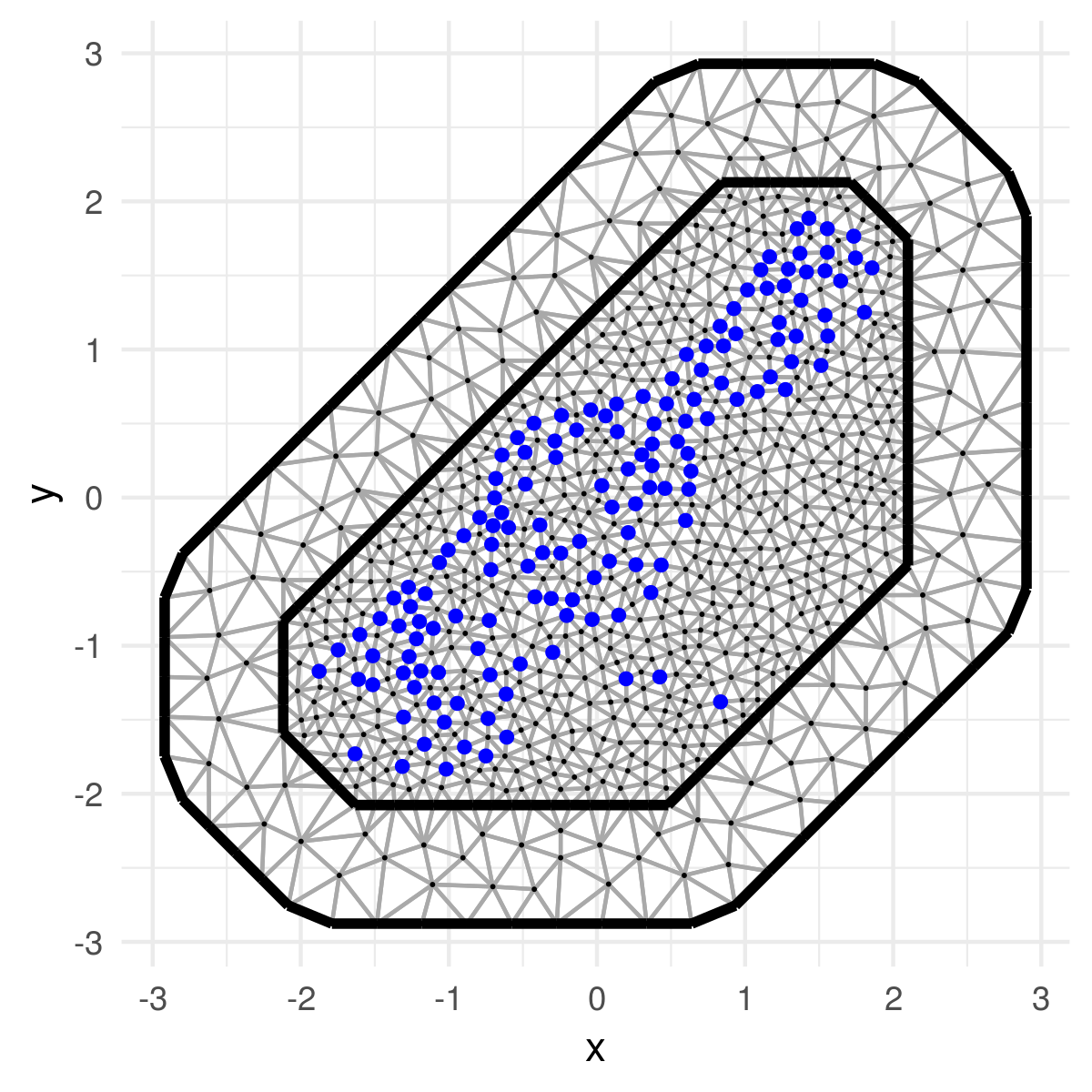
Figure 4: The SPDE mesh on top of which the stochastic partial differential equation (SPDE) is built and locations of the observations (blue dots). The coordinates represent the Rijksdriehoek (RDH) (Netherlands topographical) that have then been scaled and centered.

The ggplot_projection_shapefile command

It is convenient to visualize together the study area, mesh, and values of the random field. The corresponding objects are often of different classes. Study areas are commonly represented by spatial polygons (representing geographically relevant areas such as countries or in this case the Meuse river), while the mesh and the random field are distinct R-INLA objects. As illustrated in Figure 5, the ggplot_projection_shapefile command allows the user to visualize the study area, mesh, and values of the random field all together. This function takes as its first argument either a RasterLayer or a matrix. If a matrix is provided, an inla.mesh.projector object must also be provided as the second argument. An optional SpatialPolygonsDataFrame and inla.mesh can also then be provided as arguments spatialpolygons and mesh respectively. The function returns a ggplot object which can then be altered as usual.

data(meuse.riv)projector <- inla.mesh.projector(mesh)projection <- inla.mesh.project(projector,                                out$summary.random$spatial.field$mean)# And a shape file and scale using previous scaling valuesmeuse.riv <- sweep(meuse.riv, 2, attr(coords, "scaled:center"), FUN = "-")meuse.riv <- sweep(meuse.riv, 2, attr(coords, "scaled:scale"), FUN = "/")meuse.sr = SpatialPolygons(             list(Polygons(list(Polygon(meuse.riv)), "meuse.riv"))           )# plotpp <- ggplot_projection_shapefile(projection, projector, meuse.sr, mesh)pp + coord_equal() + ylim(-3, 3)

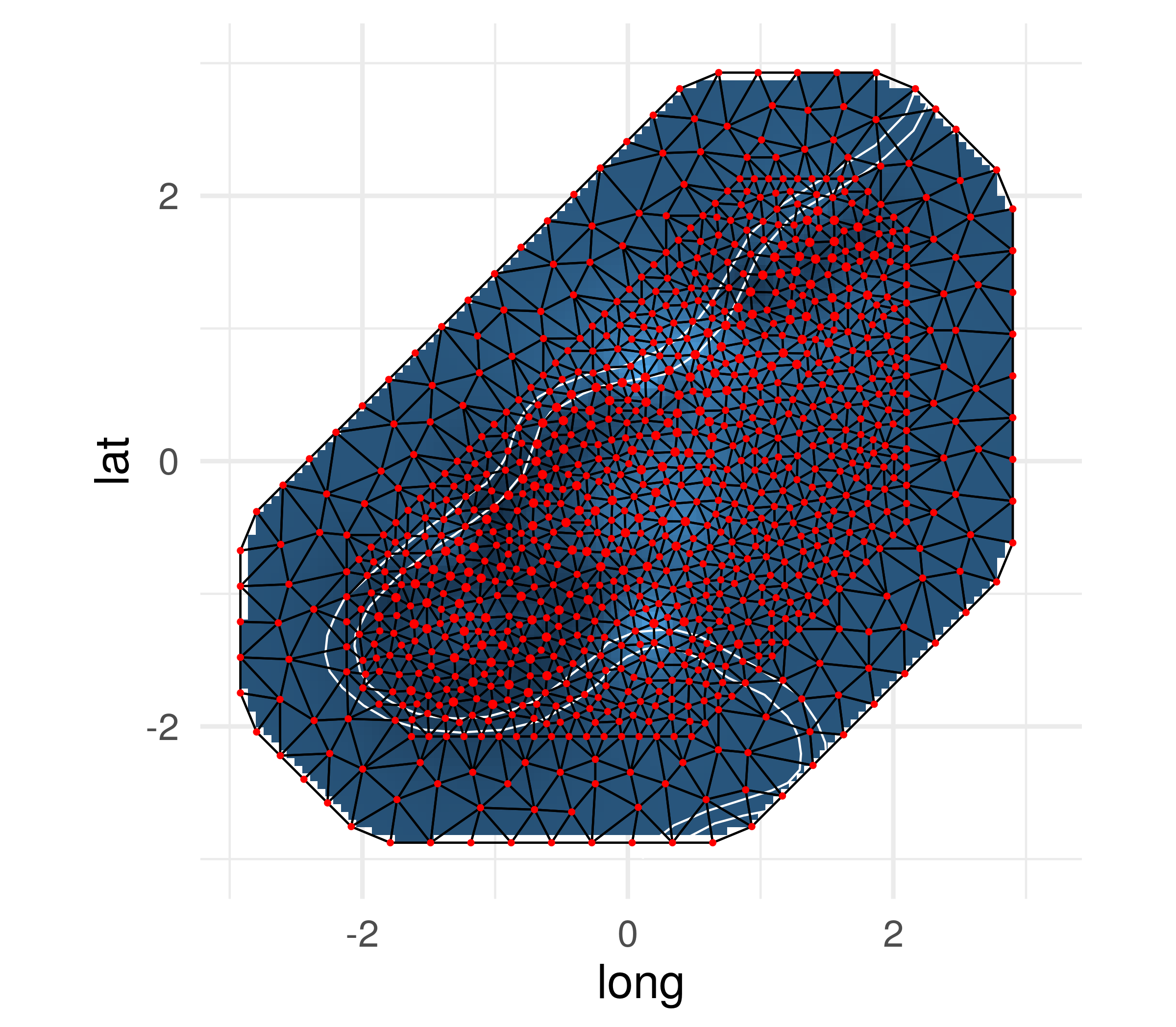
Figure 5: Visualization of the mesh with vertices (red points) and edges black triangles, study area (polygon with white border) and values of the Gaussian random field (blue shade). The coordinates represent the Rijksdriehoek (RDH) (Netherlands topographical) that have then been scaled and centered.

Spatial Leave-one-out Cross-validation

It is common to split data into training and validation sets, especially with predictive modelling purposes applied in ecological contexts (Hastie et al., 2009). A methodologically sound splitting design requires that training and validation data are independent. In the presence of spatial autocorrelation, when data held-out for validation are close in space to the training data, the independence between training and validation data can be compromised (F. Dormann et al., 2007; Hastie et al., 2009) and any model selection process may favour overly complex models with potential underestimation of the prediction errors (Mosteller and Tukey, 1977; Roberts et al., 2017). The risk of overfitting is high in flexible models that include a Gaussian spatial random component. Furthermore, the risk of under-estimating model error is particularly high when training and validation datasets are close in space but predictions are being made far from the training data.

In order to mitigate overfitting, generate more reliable error estimates and better select predictive spatial models, a common cross-validation strategy is to split data into spatial blocks (Roberts et al., 2017). Blocks consist of units of geographical area (e.g. rectangles, hexagons, disks). Block cross-validation approaches tend to provide better estimates of the errors in predictions compared to random data splits (Burman et al., 1994; Bahn and McGill, 2013; Radosavljevic and Anderson, 2014). However, if spatial blocks follow environmental gradients, for example, gradients of heavy metal concentration following a river flow, predictions can be made outside previously known combinations of predictor values from those learned from the training folds, and hence, lead to extrapolation between cross-validation folds (Snee, 1977; Zurell et al., 2012).

The spatial leave-one-out cross-validation (SLOOCV) allows for clear spatial separation between the training and the validation (left-out point) folds (Le Rest et al., 2014; Pohjankukka et al., 2017). However, users need to be cautious about defining the radius of the buffer surrounding the hold-out point. If the radius is too large, it can produce more similar training sets than blocking strategies using rectangular shapes (Hastie et al., 2009) while if it is too small, the autocorrelation in the data can still be fitted by the spatial random field.

Le Rest et al. (2014) suggested an SLOOCV approach for GLMs without spatial components fitted to spatial data. We extend this approach to explicitly spatial models fitted with R-INLA. For general information on the approach, please refer to Le Rest et al. (2014). Our suggested method (code provided below) follows three steps:

1. Remove one observation (validation set) from the initial dataset

2. Remove observations within a radius (defined by the user), so that the training set is composed of all remaining observations

3. Predict at the location of the removed observation using parameters estimated with the training set

Steps (1) to (3) are repeated $k$ times. $k$ is defined by the user and can be less than or equal to the number of data points, $n$, with $k=n$ being the case where all data points are left out once. The results are illustrated through two plots. The first plot (Figure 6) highlights the relationship between the predicted and observed values as well as displaying the mean absolute error, $\text{MAE}=\frac{1}{n}\sum_{i=1}^{n}\lvert y_{observed}-y_{predicted}\rvert$, and the root mean squared error, $\text{RMSE}=\frac{1}{n}\sum_{i=1}^{n}(y_{observed}-y_{predicted})^{2}$. The second plot displays the location and iteration number corresponding to the left-out observation(s) and corresponding surrounding disk (where observations are removed from the training data) (Figure 7). The locations of the remaining observations, that are not used as test locations are also shown so the user can see which data points will be removed in each model iteration i.e. all points within each surrounding disk will be removed for that model fit.

The command inlasloo (R code below) performs the iterative process described above. Note that the procedure performing 20 iterations on the Meuse dataset takes approximately 3-5 minutes to run on a 64Gb RAM Intel Xeon machine. It requires the user to specify the following arguments:

• dataframe: A data frame which should contain observations (rows) for each variable of interest (columns).

• The names used to defined the variables of interest are defined as strings: response y, geographic coordinates long,lat.

• The radius rad (radial distance within which observations are removed from the training set during the procedure) should be given in the unit associated with the coordinates system of the observations.

• The formula (modform) should be a formula object or a list of formula objects for testing multiple models.

• The mesh object (mesh).

• RMSE is calculated by default. The mae argument can be set to TRUE if MAE is also required.

• One or more likelihood families (bernoulli, binomial, normal, etc.) should also be set. Multiple families can be used to compare several models simultaneously, e.g. family = c('normal','bernoulli').

In order to illustrate how SLOOCV can be used to test predictive performance we compare two models fitted to the Meuse dataset. We fit the model with three covariates and a spatial random field as used above (modform) and compare it to a model with only covariates (modform2). In this case, there is little evidence that one model has better predictive performance than the other as for both MAE and RMSE the confidence intervals overlap (Figure 6).

out.field <- inla.spde2.result(out,’spatial.field’, spde, do.transf = TRUE)range.out <- inla.emarginal(function(x) x,                            out.field$marginals.range.nominal[[1]])# parameters for the SLOO processss <- 20 # sample size to process (number of SLOO runs)# define the radius of the spatial buffer surrounding the removed point.# Make sure it isn’t bigger than 25% of the study area (Le Rest et al.(2014))rad <- min(range.out, max(dist(coords)) / 4)alpha <- 0.05 # RMSE and MAE confidence intervals (1-alpha)set.seed(199)# run the function to compare both modelscv <- inlasloo(dataframe = dataframe,               long = ’long’, lat = ’lat’,               y = ’cadmium’, ss = ss,               rad = rad,               modform = list(modform, modform2),               mesh = mesh, family = ’normal’,               mae = TRUE)

Figure 6: Results of the inlasloo procedure, which illustrate the relationship between the observed response (x-axis) and the corresponding predictions (y-axis) for the full model and covariates only model. The identity function ($y=x$) is indicated by a line. Top-left: predictive scores (mean and 95% confidence interval) of the mean absolute error (mae) and root-mean-square error (rmse). Top-right: name of the model. The likelihood is a Gaussian distribution (normal), which is indicated in the x-axis label.

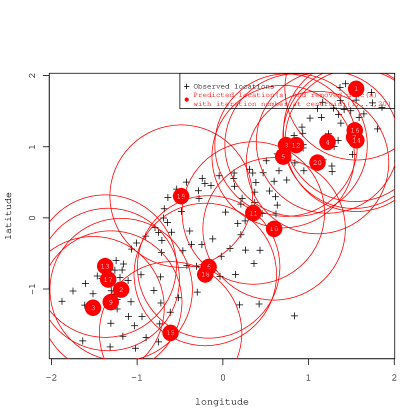
Figure 7: Visualization of the left-out observations with their corresponding iteration number (white number in red disks), radius defined by the user (red circles) and the locations of the remaining data (black crosses).

Discussion and Conclusion

The INLAutils package provides tools that allow users of R-INLA to visualise the results of their analysis more easily. We described the main graphical commands, including the autoplot command. Furthermore, we provide a concise coding framework to carry out and get an efficient visualization of the results of a spatial leave-one-out cross validation (SLOOCV) for spatial models fitted in R-INLA with the command inlasloo.

Although our SLOOCV approach allows users to compare the predictive power of several models simultaneously, some limitations are inevitable. First, predictive scores based on the likelihood (as provided in Le Rest et al. (2014) for example) are currently not included. Second, our approach only applies to purely spatial data, therefore spatio-temporal models are not considered. Future improvements of the package might include new graphical abilities and the incorporation of more models depending on the user’s requests.

-

Tim Lucas
University of Oxford, Li Ka Shing Centre for Health Information and Discovery, Big Data Institute
Oxford OX3 7LF
United Kingdom
(ORCiD: 0000-0003-4694-8107)
timcdlucas@gmail.com

Andre Python
University of Oxford, Li Ka Shing Centre for Health Information and Discovery, Big Data Institute
Oxford OX3 7LF
United Kingdom
(ORCiD: 0000-0001-8094-7226)
andre.python@bdi.ox.ac.uk

David Redding
University College London, Centre for Biodiversity and Environment Research
London WC1H 0AG
United Kingdom
(ORCiD: 0000-0001-8615-1798)
dwredding@gmail.com

References

- Bahn and McGill (2013) V. Bahn and B. J. McGill. Testing the predictive performance of distribution models. Oikos, 122(3):321–331, 2013. doi: 10.1111/j.1600-0706.2012.00299.x.
- Blangiardo and Cameletti (2015) M. Blangiardo and M. Cameletti. Spatial and spatio-temporal Bayesian models with R-INLA. John Wiley & Sons, 2015.
- Burman et al. (1994) P. Burman, E. Chow, and D. Nolan. A cross-validatory method for dependent data. Biometrika, 81(2):351–358, 1994. doi: 10.2307/2336965.
- F. Dormann et al. (2007) C. F. Dormann, J. M. McPherson, M. B. Araújo, R. Bivand, J. Bolliger, G. Carl, R. G. Davies, A. Hirzel, W. Jetz, W. Daniel Kissling, et al. Methods to account for spatial autocorrelation in the analysis of species distributional data: a review. Ecography, 30(5):609–628, 2007. doi: 10.1111/j.2007.0906-7590.05171.x.
- Gabry et al. (2019) J. Gabry, D. Simpson, A. Vehtari, M. Betancourt, and A. Gelman. Visualization in bayesian workflow. Journal of the Royal Statistical Society: Series A (Statistics in Society), 182(2):389–402, 2019. doi: 10.1111/rssa.12378.
- Hastie et al. (2009) T. Hastie, R. Tibshirani, and J. Friedman. The elements of statistical learning: data mining, inference, and prediction. Springer New York, 2009. doi: 10.1007/978-0-387-84858-7.
- Le Rest et al. (2014) K. Le Rest, D. Pinaud, P. Monestiez, J. Chadoeuf, and V. Bretagnolle. Spatial leave-one-out cross-validation for variable selection in the presence of spatial autocorrelation. Global Ecology and Biogeography, 23(7):811–820, 2014. doi: 10.1111/geb.12161.
- Lindgren (2015) F. Lindgren. Spatial Data Analysis with R-INLA with Some Extensions. Journal of Statistical Software, 63(20), 2015. doi: 10.18637/jss.v063.i20.
- Lindgren et al. (2011) F. Lindgren, H. Rue, and J. Lindström. An explicit link between Gaussian fields and Gaussian Markov random fields: the stochastic partial differential equation approach. Journal of the Royal Statistical Society: Series B, 73(4):423–498, 2011. doi: 10.1111/j.1467-9868.2011.00777.x.
- Lucas (2016) T. Lucas. palettetown: Use Pokemon Inspired Colour Palettes, 2016. URL https://github.com/timcdlucas/palettetown. R package version 0.1.1.
- Martins et al. (2013) T. Martins, D. Simpson, F. Lindgren, and H. Rue. Bayesian computing with INLA: New features. Computational Statistics & Data Analysis, 67:68–83, 11 2013. doi: 10.1016/j.csda.2013.04.014.
- Mosteller and Tukey (1977) F. Mosteller and J. W. Tukey. Data analysis and regression: a second course in statistics. Addison-Wesley Series in Behavioral Science: Quantitative Methods, 1977.
- Pebesma and Bivand (2005) E. J. Pebesma and R. S. Bivand. Classes and methods for spatial data in R. R News, 5(2):9–13, November 2005.
- Pohjankukka et al. (2017) J. Pohjankukka, T. Pahikkala, P. Nevalainen, and J. Heikkonen. Estimating the prediction performance of spatial models via spatial k-fold cross validation. International Journal of Geographical Information Science, 31(10):2001–2019, 2017. doi: 10.1080/13658816.2017.1346255.
- R Core Team (2016) R Core Team. R: A Language and Environment for Statistical Computing. R Foundation for Statistical Computing, Vienna, Austria, 2016. URL https://www.R-project.org/.
- Radosavljevic and Anderson (2014) A. Radosavljevic and R. P. Anderson. Making better MAXENT models of species distributions: complexity, overfitting and evaluation. Journal of biogeography, 41(4):629–643, 2014. doi: 10.1111/jbi.12227.
- Rikken and Van Rijn (1993) M. Rikken and R. Van Rijn. Soil Pollution with Heavy Metals: In Inquiry Into Spatial Variation, Cost of Mapping and the Risk Evaluation of Copper, Cadmium, Lead and Zinc in the Floodplains of the Meuse West of Stein, The Netherlands: Field Study Report. University of Utrecht, 1993.
- Roberts et al. (2017) D. R. Roberts, V. Bahn, S. Ciuti, M. S. Boyce, J. Elith, G. Guillera-Arroita, S. Hauenstein, J. J. Lahoz-Monfort, B. Schröder, W. Thuiller, et al. Cross-validation strategies for data with temporal, spatial, hierarchical, or phylogenetic structure. Ecography, 40(8):913–929, 2017. doi: 10.1111/ecog.02881.
- Rue et al. (2009) H. Rue, S. Martino, and N. Chopin. Approximate Bayesian inference for latent Gaussian models by using integrated nested Laplace approximations. Journal of the Royal Statistical Society: Series B, 71(2):319–392, 2009. doi: 10.1111/j.1467-9868.2008.00700.x.
- Snee (1977) R. D. Snee. Validation of regression models: methods and examples. Technometrics, 19(4):415–428, 1977. doi: 10.2307/1267881.
- Wilke (2019) C. O. Wilke. cowplot: Streamlined Plot Theme and Plot Annotations for ’ggplot2’, 2019. URL https://CRAN.R-project.org/package=cowplot. R package version 0.9.4.
- Zurell et al. (2012) D. Zurell, J. Elith, and B. Schröder. Predicting to new environments: tools for visualizing model behaviour and impacts on mapped distributions. Diversity and Distributions, 18(6):628–634, 2012. doi: 10.1111/j.1472-4642.2012.00887.x.
-