Reducing Data Motion to Accelerate the Training of Deep Neural Networks

Abstract

The use of Deep Neural Networks (DNNs) is becoming ubiquitous in many areas due to their exceptional pattern detection capabilities. For example, deep learning solutions are coupled with large scale scientific simulations to increase the accuracy of pattern classification problems and thus improve the quality of scientific computational models. Despite this success, deep learning methods still incur several important limitations: the DNN topology must be set by going through an empirical and time-consuming process, the training phase is very costly and the latency of the inference phase is a serious limitation in emerging areas like autonomous driving.

This paper reduces the cost of DNNs training by decreasing the amount of data movement across heterogeneous architectures composed of several GPUs and multicore CPU devices. In particular, this paper proposes an algorithm to dynamically adapt the data representation format of network weights during training. This algorithm drives a compression procedure that reduces data size before sending them over the parallel system. We run an extensive evaluation campaign considering several up-to-date deep neural network models and two high-end parallel architectures composed of multiple GPUs and CPU multicore chips. Our solution achieves average performance improvements from 6.18% up to 11.91%.

I Introduction

The use of Deep Neural Networks (DNNs) is becoming ubiquitous in areas like computer vision (e.g., image recognition and object detection) [1, 2], speech recognition [3], language translation [4], and many more [5]. DNNs provide very competitive pattern detection capabilities and, more specifically, Convolutional Neural Networks (CNNs) classify very large image sets with remarkable accuracy [6]. Indeed, DNNs already play a very significant role in the large production systems of major IT companies and research centers, which has in turn driven the development of advanced software frameworks for the deep learning area [7] as well as DNN-specific hardware accelerators [8, 9]. As an example, deep learning solutions are being coupled with physical computational models for solving pattern classification problems in the context of large-scale climate simulations [10]. Despite all these accomplishments, deep learning models still suffer from several fundamental problems: the neural network topology is determined through a long and iterative empirical process, the training procedure has a huge cost in terms of time and computational resources, and the inference process of large network models incurs considerable latency to produce an output, which is not acceptable in domains requiring real-time responses like autonomous driving.

To deal with the large quantity of Floating Point computations required to train a DNN, GPUs are usually employed [11]. They exploit the large amount of data-level parallelism of deep learning workloads. Although GPUs and other hardware accelerators have been successfully employed to boost the training process, data exchanges involving different accelerators may incur significant performance penalties.

This paper describes and evaluates a method that exploits DNNs tolerance to data representation formats smaller than the commonly used 32-bit Floating Point (FP) standard [12, 13]. Our method accelerates the training of DNNs by reducing the cost of data transfers across heterogeneous high-end architectures integrating multiple GPUs without deterioration on the training accuracy. Our solution is designed to efficiently use the incoming bandwidth of the GPU accelerators. It relies on an adaptive scheme that dynamically adapts the data representation format required by each DNN layer and compresses network parameters before sending them over the parallel system. This paper makes the following contributions:

• It proposes the Adaptive Weight Precision (AWP) algorithm, which dynamically adapts the numerical representation of DNN weights during training. AWP relies on DNNs’ tolerance for reduced data representation formats. It defines the appropriated data representation format per each network layer during training without hurting network accuracy.

• It proposes the Approximate Data Transfer (ADT) procedure to compress DNN’s weights according to the decisions made by the AWP algorithm. ADT relies on both thread- and SIMD-level parallelism and is compatible with architectures like IBM’s POWER or x86. ADT is able to compress large sets of weights with minimal overhead, which enables the large performance benefits of our approach.

• It evaluates ADT and AWP on two high-end systems: The first is composed of two x86 Haswell multicore devices plus four NVIDIA Tesla GK210 GPU accelerators and the second system integrates two POWER9 chips and four NVIDIA Volta V100 GPUs. Our evaluation considers the Alexnet [1], the VGG [14] and the Resnet [15] network models applied to the ImageNet ILSVRC-2012 dataset [16]. Our experiments report average performance benefits of 6.18% and 11.91% on the x86 and the POWER systems, respectively.

Many proposals describe how data representation formats smaller than the 32-bit Floating Point IEEE standard can be applied to deep learning workloads without hampering their accuracy [17, 12, 18]. This paper presents the first approach that uses reduced data formats to minimize data movement during DNN training in heterogeneous high-end systems, which are extensively used to run deep learning workloads [11].

This paper is structured as follows: Section II describes our first contribution, the Adaptive Weight Precision algorithm (AWP). Section III details the Approximate Data Transfer (ADT) procedure. Section IV explains the experimental setup of this paper. Section V describes the experiments we conduct to evaluate AWP and ADT on three state-of-the-art neural networks. Section VI describes the most relevant related work. Finally, Section VII summarizes the conclusions of this paper.

II The Adaptive Weight Precision (AWP) Algorithm

The Adaptive Weight Precision (AWP) algorithm relies on the tolerance of DNNs to data representation formats smaller than the 32-bit Floating Point standard. Indeed, previous work indicates that, unlike scientific codes focused on solving partial differential equations or large linear systems, neural networks do not always require 32-bit representation during training [17, 12]. Even more, adding stochastic noise to certain variables during the learning phase improves DNNs accuracy [19, 20, 21]. Nevertheless, when facing unknown scenarios in terms of new workloads or parameter settings, the data representation requirements of DNNs are non-trivial to be determined and, to make things more complicated, they may change as the training phase progresses.

The AWP algorithm dynamically determines data representation requirements per each network layer by monitoring the evolution of the $l^{2}$-norm of the weights. AWP identifies the number of bits required to represent DNNs weights and guarantees the progress of the training process. AWP assigns the same data representation format to all weights belonging to a certain network layer. The training starts with a small data representation that is independently increased for each layer.

Algorithm 1 Adaptive Weight Precision (AWP) Algorithm

1:BitsPerLayer := [$B_{0},B_{1},\ldots,B_{NumLayers}$] $\triangleright$ List storing the number of bits corresponding to the data representation of each layer

2:IntervalCounter := [0, 0, $\ldots$, 0] $\triangleright$ List storing the number of times the relative change rate fails to meet the threshold per layer

3:for batch := 0 …NumBatches do

4:     Apply backpropagation to batch

5:     for layer := 0 …NumLayers do

6:         $\delta:=\frac{(|\text{W}_{batch,layer}|-|\text{W}_{batch-1,layer}|)}{|\text{W}_{batch-1,layer}|}$

7:         if $\delta$ < T then

8:              $\text{IntervalCounter}_{layer}$ += 1

9:         end if

10:         if $\text{IntervalCounter}_{layer}$ == INTERVAL then

11:              $\text{BitsPerLayer}_{layer}$ += N

12:              $\text{IntervalCounter}_{layer}$ := 0

13:         end if

14:     end for

15:end for

Algorithm 1 displays a pseudo-code description of AWP. Once the backpropagation process has been applied to a given batch, AWP iterates over all network layers. The algorithm computes per each batch and network layer the $l^{2}$-norm of all its weights’ values and derives the relative change rate $\delta$ of the $l^{2}$-norm with regard to the previously processed batch. For the batch $i$, the change rate is defined as $\delta_{i}=(|W_{i}|-|W_{i-1}|)/|W_{i-1}|$, where $W_{i}$ is the vector of weights of a certain layer while batch $i$ is processed. Every time the change rate is below a given threshold T for a certain layer, the algorithm accounts for it by increasing the $IntervalCounter$ parameter. The algorithm increases $N$ bits of precision if the change rate is below T during a certain number of batches defined by the parameter INTERVAL and sets the $IntervalCounter$ parameter of the corresponding layer to zero. Section V-A describes how we determine the values of parameters T, INTERVAL, and N.

III The Approximate Data Transfer (ADT) Procedure

The Approximate Data Transfer (ADT) procedure compresses network’s weights before they are transferred to the GPUs. In the context of DNNs training on heterogeneous multi-GPU nodes, CPU multicore devices are typically responsible for orchestrating the parallel run and updating DNN parameters. Once the process of a batch starts, the updated parameters including the weights $W$ are sent to each GPU. If the set of parameters does not fit in GPUs’ main memory, they are sent on several phases as the different GPUs need them. The different samples of each batch are evenly distributed across all GPUs. Therefore, each GPU computes its contribution to the gradient $\Delta W$ by processing its corresponding set of samples. The CPU multicore subsequently gathers all contributions to the gradient and uses them for weight updates $W\leftarrow W-\mu(\frac{1}{n}\sum_{i}^{n}\Delta W_{i})$, where $\mu$ is the learning rate.

Data movement involving different GPU devices increases as the network topology becomes more complex or the number of training samples grows, which can saturate the system bandwidth and become a major performance bottleneck. This paper mitigates this issue by compressing network weights before they are sent to the GPU devices. The AWP algorithm described in Section II determines, for all weights belonging to a particular network layer, the number of bits to send. In this context, to efficiently compress and decompress network weights, ADT uses of two procedures that constitute its fundamental building blocks. These procedures are complementary and applied either before or after data transfers to GPUs.

• Bitpack compresses the weights discarding the less significant bits on the CPU side;

• Bitunpack converts the weights back to the IEEE-754 32-bit Floating Point format on the GPUs.

Figure 1 provides an example including a multicore CPU and two GPU devices to describe the way both Bitpack and Bitunpack procedures operate. All neural network parameters (weights and biases) are updated at the CPU level, which is where the Bitpack procedure takes place. We do not apply the Bitpack procedure to the network biases since we do not observe any significant performance benefit from compressing them. Since each output neuron requires just one bias parameter, the total number of them is significantly smaller than the total number of weights. At the beginning of each SGD iteration the compressed weights are sent to each GPU together with the biases and the corresponding training samples. Each GPU uncompresses the weights, builds the neural network model, and computes its specific contribution to the gradient. These contributions are sent to the CPU, which gathers them, computes the gradient, and updates network parameters.

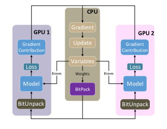
Figure 1: The ADt on a 2-GPU system. Variables include: weights which go through the ADt procedure and biases which are sent directly to the GPUs to build the network model together with the unpacked weights.

The Bitpack operation runs on CPU multicore devices. To boost Bitpack we use OpenMP [22] and Single-Instruction Multiple Data (SIMD) intrinsics. OpenMP is used to run Bitpack on several threads. The use of SIMD instructions allows Bitpack to operate at the SIMD register level, which avoids incurring large performance penalties in the process of producing the reduced-size weights. We implement two versions of Bitpack. One version uses Intel’s AVX2 [23] instruction set and the other one relies on AltiVec [24]. Bitpack can be implemented on top of any SIMD instruction set architecture supporting simple byte shuffling instructions at the register level.

The Bitunpack procedure runs on the GPUs. It can be trivially parallelized since each weight is mapped to a single 32-bit FP variable, which means that GPUs can process a large amount of weights simultaneously and efficiently build the DNN model. In fact, Bitunpack incurs negligible overhead as Section V-G shows.

ADT manipulates the internal representation of network weights by discarding some bits. We use the standard 32-bit IEEE-754 single-precision Floating Point format  [25] (1 bit sign, 8 bits exponent and 23 bits mantissa) for all the computation routines. The Bitpack method considers network weights as 32-bit words where rounding to $N$ bits means discarding the lowest $32-N$ bits.

Algorithm 2 High Level Pseudo-code Version of Bitpack

1:W $\triangleright$ Array of 32-bit Floating Point values containing weights

2:Pw $\triangleright$ Array containing the reduced precision weights

3:RoundTo $\triangleright$ Number of bytes to keep per weight

4:POffset := 0 $\triangleright$ Indicates the current size (in bytes) of Pw

5:for weight in W do

6:     Pw[POffset : POffset+RoundTo] := weight[0 : RoundTo] $\triangleright$ Copy most significant RoundTo bytes to Pw

7:     POffset := POffset + RoundTo

8:end for

III-A Bitpack

A high-level version of the Bitpack procedure in terms of pseudo-code is illustrated by Algorithm 2. The algorithm requires a couple of arrays: the input array $W$, which contains all the weights of a certain network layer, and an output array $Pw$, which stores the compressed versions of these weights. The algorithm goes through the entire $W$ input array and, per each weight, it copies the most significant $RoundTo$ bytes to the output array $Pw$. Our Bitpack implementation manipulates data at the byte granularity. We do not observe significant performance benefits when operating at finer granularity in the experiments we run. The AWP algorithm described in Section II determines the data representation format per each network layer. The number of bits of the chosen format is rounded to the nearest number of bytes that retains all of its information (E.g., if AWP provides the value 14, $RoundTo$ will be set to 2 bytes). The $Pw$ array is sent to the GPUs once the Bitpack procedure finishes compressing network weights.

Deep networks usually contain tens or even hundreds of millions of weights [1, 26, 14], which makes any trivial implementation of Algorithm 2 not applicable in practice. We mitigate compression costs by observing that Algorithm 2 is trivially parallel since processing one weight just requires the $RoundTo$ parameter. Algorithm 3 shows how to parallelize the Bitpack procedure by using OpenMP threads. Each thread takes care of a certain portion of the $Pw$ array.

Algorithm 3 Bitpack with OpenMP

1:W $\triangleright$ Array of 32-bit Floating Point values containing weights

2:Pw $\triangleright$ Array containing the reduced precision weights

3:RoundTo $\triangleright$ Number of bytes to keep per weight

4:NumThreads $\triangleright$ Number of OpenMP threads

5:#pragma omp parallel for

6:for weight in W do

7:     POffset := Corresponding position in Pw

8:     Pw[POffset : POffset+RoundTo] := weight[0 : RoundTo] $\triangleright$ Copy the most significant RoundTo bytes to Pw

9:end for

III-B Single Instruction Multiple Data Bitpack

Since all weights within one layer are processed in the same way by the Bitpack procedure, we can leverage Single Instruction Multiple Data (SIMD) instructions to vectorize it. Most state-of-the-art architectures implement SIMD instruction set: IBM’s AltiVec [24], Intel’s Advanced Vector Extensions (AVX) [23], and ARM’s Neon [27]. In our experiments we use Intel’s AVX2 [23], which implements a set of SIMD instructions operating over 256-bit registers, and IBM’s AltiVec instruction set [24], which has SIMD instructions operating over 128-bit registers. Section IV describes the specific details of our evaluation considering both x86 and POWER architectures.

Figure 2 shows the byte-level operations of SIMD-based Bitpack applied to eight 32-bit weights and implemented with AVX2. The RoundTo parameter is set to 3, which implies discarding the last 8 bits of each weight since the target data representation is 24-bit long. First, eight 32-bit Floating Point weights are loaded to a 256-bit register. In the next step, we use _mm256_shuffle_epi8 to shuffle the least significant eight bits of each weight to the least significant bits of their respective 128-bit lane (see the grey area of Figure 2 Step 2) and pack the rest of the bits together. Afterwards we use _mm256_permutevar8x32_epi32 to do the same operation across the two 128-bit lanes. Finally, we use _mm256_maskstore_epi32 to just store the resulting 192 bits to the target array. Not all AVX2 instructions operate over the entire 256-bit register. Instead, many of them conceive the register as two 128-bit lanes and operate on them separately. This is the reason way we can not carry out Steps 2 and 3 by using a single AVX2 instruction.

[bitwidth=0.75em, bitformatting=,endianness=big]32 2 Step 1: Load 8 32-bit weights into a 256-bit AVX2 register. (_mm256_loadu_si256)
4$H_{3..0}$&$G_{3..0}$$F_{3..0}$ $E_{3..0}$$D_{3..0}$ $C_{3..0}$$B_{3..0}$$A_{3..0}$
0,3,7,11,15,19,23,27,31
2 Step 2: Pack weights on the 2 128-bit lanes. (_mm256_shuffle_epi8)
3$H_{3..1}$ & 3$G_{3..1}$ 3$F_{3..1}$ 3$E_{3..1}$ 4 3$D_{3..1}$ 3$C_{3..1}$ 3$B_{3..1}$ 3$A_{3..1}$ 4
0,3,6,9,12,15,19,22,25,28,31
2 Step 3: Pack the 8 weights together by rearranging 32-bit across 128-lanes. (_mm256_permutevar8x32_epi32)
3$H_{3..1}$ 3$G_{3..1}$ 3$F_{3..1}$ 3$E_{3..1}$ 3$D_{3..1}$ 3$C_{3..1}$ 3$B_{3..1}$ 3$A_{3..1}$ 8
0, 7, 10, 13, 16, 19, 22, 25, 28, 31
2 Step 4: Store the most significant 24 bytes (192 bits) of data into the target array. (_mm256_maskstore_epi32)

Figure 2: Bitpack implemented with AVX2, RoundTo=3

Algorithm 4 Bitpack with OpenMP + AVX2

1:W $\triangleright$ Array of 32-bit Floating Point values containing weights

2:Pw $\triangleright$ Array containing the reduced precision weights

3:RoundTo $\triangleright$ Number of bytes to keep per weight

4:#pragma omp parallel for

5:for weights in W do

6:     _mm256_loadu_si256 $\triangleright$ Load 8 32-bit weights

7:     _mm256_shuffle_epi8 $\triangleright$ Compress at each 128-bit lane

8:     _mm256_permutevar8x32_epi32 $\triangleright$ Shuffle the compressed weights into the most significant bits

9:     _mm256_maskstore_epi32 $\triangleright$ Store compressed weights to the target array

10:end for

Algorithm 5 Bitunpack on GPU

1:Pw $\triangleright$ Array containing compressed weights

2:W $\triangleright$ Array of 32-bit Floating Point values containing weights

3:RoundTo $\triangleright$ The number of bytes that are going to be kept

4:for UnitId := 0 …NumUnit do

5:     Distribute W and Pw across all the computation units in the GPU

6:     POffset := 0

7:     for weight in W do

8:         weight := Pw[POffset : POffset+RoundTo] $\ll$ (4 - RoundTo) * 8

9:         POffset := POffset + RoundTo

10:     end for

11:end for

Algorithm 4 summarizes our implementation of the Bitpack procedure with AVX2. It exploits two-level parallelism: first, the input array of weights is distributed across several threads. Second, within each thread, the compression of each eight 32-bit weights subset is performed at the register level by means of byte shuffling instructions. This sophisticated procedure exploiting parallelism at both thread and SIMD register levels uses all the available hardware resources and avoids costly memory accesses.

III-C Bitunpack

Once data in reduced-size format reaches the target GPU, the Bitunpack procedure immediately restores them into their original IEEE-754 32-bit Floating Point format. We display pseudo-code describing this process in Algorithm 5. Bitunpack reads the reduced-sized weights from array $Pw$ and assigns additional bits to them. Bitunpack gives zero values to these additional bits. We distribute the Bitunpack process across the whole GPU, which enables an extremely parallel scheme exploiting GPUs manycore architecture.

The Bitunpack routine is developed using CUDA [28]. Our code runs in parallel on $N$ CUDA threads and the CUDA runtime handles the dynamic mapping between threads and the underlying GPU compute units. Since each thread involved in the parallel run targets a different portion of the $Pw$ array, our Bitunpack procedure exposes a large amount of parallelism to the numerous computing units integrated into high-end GPU devices.

IV Experimental Setup

The experimental setup considers a large image dataset, three state-of-the-art neural network models and two high-end platforms. The following sections describe all these elements in detail.

IV-A Image Dataset

We consider the ImageNet ILSVRC-2012 dataset [16]. The original ImageNet dataset includes three sets of images of 1000 classes each: training set (1.3 million images), validation set (50,000 images) and testing set (100,000 images). We consider a subset of 200 classes for the wide evaluation we show in Sections V-B, V-C, V-D, and V-E, which considers three different network models, three different batch sizes per model, two different platforms and three different training approaches. Considering 1000 classes makes the training process around 170 hours long, which is prohibitively expensive for this large experimental campaign. We consider the whole ImageNet data set in the experiments we show in Section V-F, which confirm the trends observed when considering the reduced data set. For the rest of this paper, we refer to the 200 and 1000 classes datasets as ImageNet200 and ImageNet1000, respectively. Since it is a common practice [14], we evaluate the ability of a certain network in properly dealing with the ImageNet ILSVRC-2012 dataset in terms of the top-5 validation error computed over the validation set.

IV-B DNN Models and Training Parameters

We apply the AWP algorithm along with the ADT procedure on three state-of-the-art DNN models: a modified version of Alexnet [1] with an extra fully-connected layer of size 4096, the configuration A of the VGG model [14] and the Resnet network [15]. All hidden layers are equipped with a Rectified Linear Units (ReLU) [1]. The exact configurations of the three neural networks are shown in Table I. The Alexnet model is composed of 5 convolutional layers and 4 fully-connected ones, VGG contains 8 convolutional layers and 3 fully-connected ones and Resnet is composed of 33 convolutional layers and a single fully-connected one.

TABLE I: Neural network configurations: The convolutional layer parameters are denoted as “conv<receptive field size>-<number of channels>”. The ReLU activation function is not shown for brevity. The building blocks of Resnet and the number of times they are applied are shown in a single cell.

Alexnet	VGG	Resnet-34
input(224x224 RGB image)
conv11-64	conv3-64	conv7-64
maxpool
conv5-192	conv3-128	conv3-64 conv3-64 x3
maxpool
conv3-384	conv3-256 conv3-256	conv3-128 conv3-128 x4
maxpool
conv3-384	conv3-512 conv3-512	conv3-256 conv3-256 x6
maxpool
conv3-256	conv3-512 conv3-512	conv3-512 conv3-512 x3
maxpool		avgpool
FC-4096
FC-4096 FC-4096	FC-4096
FC-200
softmax

We use momentum SGD [29] to guide the training process with momentum set to 0.9. The training process is regularized by weight decay and the $L_{2}$ penalty multiplier is set to $5\times 10^{-4}$. We apply a dropout regularization value of 0.5 to fully-connected layers. We initialize the weights using a zero-mean normal distribution with variance $10^{-2}$. The biases are initialized to $0.1$ for Alexnet and $0$ for both VGG and Resnet networks. For the Alexnet and VGG models we consider training batch sizes of 64, 32 and 16. To train the largest network we consider, Resnet, we consider batch sizes of 128, 64 and 32. The 16 batch size incurs in a prohibitively expensive training process for Resnet and, therefore, we do not use it in our experimental campaign.

For Alexnet we set the initial learning rate to $10^{-2}$ for the 64 batch size and decrease it by factors of 2 and 4 for the 32 and 16 batch sizes, respectively. In the case of VGG we set the initial learning rate to $10^{-2}$ for the 64, 32 and 16 batch sizes, as in the state-of-the-art [14]. In the case of Resnet the learning rate is $10^{-2}$ for the batch size of 32 and 0.1 for the rest. For all network models we apply exponential decay to the learning rate throughout the whole training process in a way the learning rate decays every 30 batches by a factor of 0.16, as previous work suggests [26]. For Resnet we obtain the best results when adapting precision at the Resnet building block level [15] instead of doing it in a per-layer basis.

IV-C Implementation

Our code is written in Python on top of Google Tensorflow [7]. Tensorflow is a data-flow numerical library where computations are driven by a computational graph that defines their order. It supports NVIDIA’s NCCL library.

To enable the use of both Bitpack and Bitunpack routines, we integrate them into Tensorflow using its C++ API. Tensorflow executes the two routines before sending the weights from the CPU to the GPU and right after receiving the weights on the GPU side, respectively. The Bitpack routine is implemented using the OpenMP 4.0 programming model. There are two versions of this routine using either Intel’s AVX2 or IBM’s AltiVec instructions, as explained in Section III. Bitunpack is implemented using CUDA 8.0 and CUDA 10.0 respectively on the two platforms [28].

IV-D Hardware Platforms

We conduct our experiments on two clusters featuring the x86 and POWER architectures. The x86 machine is composed of two 8-core Intel Xeon ®E5-2630 v3 (Haswell) at 2.4 GHz and a 20 MB L3 shared cache memory each. It is also equipped with two Nvidia Tesla K80 accelerators, each of which hosts two Tesla GK210 GPUs. It has 128 GB of main memory, distributed in 8 DIMMs of 16 GB DDR4 @ 2133 MHz. The 16-core CPU and the four GPUs are connected via a PCIe 3.0 x8 8GT/s. The operating system is RedHat Linux 6.7. Overall, the peak performance of the two 8-core sockets plus the four Tesla GK210 GPUs is 6.44 TFlop/s.

The POWER machine is composed of two 20-core IBM POWER9 8335-GTG at 3.00 GHz. It contains four NVIDIA Volta V100 GPUs. Each node has 512 GB of main memory, distributed in 16 DIMMS of 32 GB @ 2666 MHz. The GPUs are connected to the CPU devices via a NVIDIA NVLink 2.0 interconnection [30]. The operating system is RedHat Linux 7.4. The peak performance of the two 20-core sockets plus the four V100 GPUs is 28.85 TFlop/s.

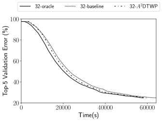
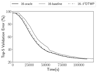
Figure 3: Alexnet training considering 32 and 16 batch sizes. The two plots show the top-5 validation error evolution of baseline, oracle and $A^{2}$DTWP.

V Evaluation

In this section we evaluate the capacity of the AWP algorithm and the ADT procedure to accelerate DNNs training. We show how our proposals are able to accelerate the training phase of relevant DNN models without reducing the accuracy of the network.

V-A Methodology

Our experimental campaign considers batch sizes of 64, 32 and 16 for the Alexnet and VGG models and 128, 64 and 32 for the Resnet network. For each model and batch size, the baseline run uses the 32-bit Floating Point precision for the whole training. The data represention formats we consider to transfer weights from the CPU to the GPU are: 8-bit (1 bit for sign, 7 bits for exponent), 16-bit (1 bit for sign, 8 for exponent, 7 for mantissa), 24-bit (1 bit for sign, 8-bits for exponent and 15 bits for mantissa) and 32-bits (1 bit for sign, 8 bits for exponent and 23 bits for mantissa). We train the network models with dynamic data representation by applying the AWP algorithm along with the ADT procedure. We denote this approach combining ADT and AWP as $A^{2}$DTWP. For each DNN and batch size, we select the data representation format that first reaches the 35%, 25% and 15% accuracy thresholds for Resnet, Alexnet and VGG, respectively, and we denote this approach as oracle. For the case of the oracle approach, data compression is done via ADT. The closer $A^{2}$DTWP is to oracle, the better is the AWP algorithm in identifying the best data representation format.

During training we sample data in terms of elapse time and validation error every 4000 batches. The total number of training batches corresponding to the whole ImageNet200 dataset are 16020, 8010, 4005 and 2002 for batch sizes 16, 32, 64 and 128, respectively. The values of $AWP$ parameters $T$, $INTERVAL$, and $N$ are determined in the following way: In the case of $T$ we monitor the execution of several epochs until we observe a drop in the validation error. We then measure the average change, considering all layers, of weights’ $l^{2}$-norm during this short monitoring period. The obtained values of $T$ are $-5\times 10^{-2}$, $-2\times 10^{-3}$ and $-2\times 10^{-5}$ for Alexnet, VGG and Resnet, respectively. We set the $INTERVAL$ parameter to $4000$ for both AlexNet and VGG and $2000$ for Resnet. These values correspond to a single batch (for the ImageNet200 dataset and batch sizes 64 and 128) and avoid premature precision switching due to numerical fluctuations. We set $N$ to $8$ since the smallest granularity of our approach is 1 byte. AWP initially applies 8-bit precision to all layers. We use ImageNet200 in Sections V-B,  V-C,  V-D,  V-E, and  V-G. Section V-F uses ImageNet1000.

V-B Evaluation on Alexnet

The evaluation considering the Alexnet model on the x86 system is shown in Figure 3, which plots detailed results considering batch sizes of 32 and 16, and Figure 4, which shows the total execution time of the oracle and $A^{2}$DTWP policies normalized to the baseline for the 64, 32 and 16 batch sizes on both the x86 and the POWER systems. The two plots of Figure 3 depict how the validation error of the baseline, oracle, and $A^{2}$DTWP policies evolves over time for the 32 and the 16 batch sizes until the 25% accuracy is reached.

It can be observed in the left-hand side plot of Figure 3 how the oracle and the $A^{2}$DTWP approaches are 10.82% and 6.61% faster than the baseline, respectively, to reach the 25% top-5 validation error when using a 32 batch size. The right-hand side plot shows results considering a 16 batch size. The improvements achieved by the oracle and $A^{2}$DTWP approaches are 11.52% and 10.66%, respectively. This demonstrates the efficiency of the ADT procedure in compressing and decompressing the network weights without undermining the performance benefits obtained from sending less data from the CPU device to the GPU. It also demonstrates the capacity of AWP to quickly identify the best data representation format per layer.

Figure 4 shows the normalized execution time of the oracle and $A^{2}$DTWP policies with respect to the 32-bit FP baseline on the x86 and the POWER systems. The top chart reports performance improvements of 10.75%, 6.51%, and 0.59% for batch sizes 16, 32 and 64 in the case of Alexnet runnig on the x86 system. For the 64 batch size, the marginal gains of $A^{2}$DTWP over the baseline are due the poor performance of the 8-bits format employed by $A^{2}$DTWP at the beginning of the training process. This format does not contribute to reduce the validation error for the 64 batch case, which makes the $A^{2}$DTWP policy to fall behind the baseline at the very beginning of the training process. Although $A^{2}$DTWP eventually increases its accuracy and surpases the baseline, it does not provide the same significant performance gains for Alexnet as the ones observed for batch sizes 16 and 32.

$A^{2}$DTWP performance improvements on the POWER system in the case of Alexnet are 18.61%, 14.25% and 10.01% with respect to the baseline for batch sizes 16, 32 and 64, respectively. $A^{2}$DTWP achieves better performance increases on the POWER system than x86 since its CPU to GPU bandwidth per GPUs flop/s ratio, 0.86 Bytes per Flop, is significantly slower than the x86 system ratio, 1.22 Bytes per Flop. This ratio expresses the maximum CPU to GPU bandwith per GPUs flop/s, which indicates the capacity to keep GPUs busy. Since this capacity is smaller in the POWER system than in the x86 machine, our methodology achieves larger improvements when deployed on POWER.

V-C Evaluation on VGG

Figure 4 illustrates the normalized execution time of $A^{2}$DTWP and oracle with respect to the baseline for VGG considering batch sizes of 16, 32 and 64 on the x86 and POWER systems. When applied to the VGG model on the x86 system, $A^{2}$DTWP outperforms the 32-bit Floating Point baseline by 12.88%, 5.02% and 7.31% for batch sizes 64, 32 and 16, respectively. Despite the relatively low performance improvement achieved by the $A^{2}$DTWP technique when applied to the 32 batch size, $A^{2}$DTWP reaches substantial enhancements over the baseline in all considered scenarios.

The performance improvements observed when training VGG on the POWER system are even higher. $A^{2}$DTWP outperforms the baseline by 28.21%, 20.19% and 11.13% when using the 16, 32 and 64 batch sizes, respectively. The performance improvement achieved on the POWER system are larger than the ones observed for x86 since it has less CPU to GPU bandwitdh per flop/s. We observe the same behavior for Alexnet, as Section V-B indicates.

V-D Evaluation on Resnet

We display the normalized execution time of the $A^{2}$DTWP and the oracle policies when applied to the Resnet model using batch sizes of 128, 64 and 32 in Figure 4. On the x86 system, $A^{2}$DTWP beats the 32-bit Floating Point baseline by 4.94%, 4.39% and 3.11% for batch sizes of 128, 64 and 32, respectively, once a top-5 validation error of 30% is reached. The relatively low performance improvement achieved in the case of 32 batch size is due to a late identification of a competitive numerical precision, as it happens in the case of VGG and batch size 32.

The performance gains on the POWER system display a similar trend as the ones achieved on x86. While they show the same low improvement for the 32 batch size, 2.12%, $A^{2}$DTWP achieves 6.92% and 11.54% performance gains for batch sizes 64 and 128, respectively. $A^{2}$DTWP achieves the largest performance improvement with respect to the 32-bit baseline when run on the POWER system due to the reasons described in Sections V-B and V-C.

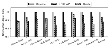
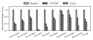
Figure 4: Normalized execution times of the $A^{2}$DTWP and the oracle policies with respect to the baseline. Results obtained on the x86 system appear in the upper plot while the evaluation on the POWER system appears at the bottom.

V-E Average Performance Improvement

The average performance improvement of $A^{2}$DTWP over the baseline considering the Alexnet, VGG and Resnet models reach 6.18% and 11.91% on the x86 and the POWER systems, respectively. As we explain in previous sections, $A^{2}$DTWP obtains larger improvements on the POWER system than on x86 due to its smaller CPU to GPU Byte per Flop ratio. This ratio is expected to decrease in future systems since flop/s will increase more than bandwdith, which indicates the potential of $A^{2}$DTWP to achieve even larger performance gains in future systems.

The combination of the AWP algorithm and the ADT procedure properly adapts the precision of each network layer and compresses the corresponding weigths with a minimal overhead. The large performance improvement obtained while training deep networks on two high-end computing systems demonstrate the effectiveness of $A^{2}$DTWP.

V-F Experiments with ImageNet1000

We run experiments considering ImageNet1000 to confirm they display the same trends as executions with ImageNet200. The experimental setup of the evaluation considering ImageNet1000 is the same as the one we use for ImageNet200, including training and $AWT$ parameters, which are described in Sections IV-B and V-A. We consider batch sizes that produce the fastest 32-bit FP training for each one of the network models: 64, 64, and 128 for Alexnet, VGG and Resnet, respectively.

Figure 5 displays results corresponding to the experimental campaign with ImageNet1000 on the x86 system. In the x-axis we display different epoch counts for each one of the three models: 4, 8, 12, 16, and 20 epochs for Alexnet; 2, 4, 6, and 8 for VGG; and 4, 8, 12, and 16 epochs for Resnet. The y-axis displays the normalized elapsed time of $A^{2}$DTWP with respect to the the 32-bit Floating Point baseline per each model and epoch count. For the case of Alexnet with batch size 64, $A^{2}$DTWP is slightly faster than the baseline as it displays a normalized execution time of 0.995, 0.992, 0.992, 0.996, and 0.990 after 4, 8, 12, 16 and 20 epochs, respectively. Figure 4 also reports small gains for the case of Alexnet with batch size 64, which confirms that experiments with ImageNet1000 show very similar trends as the evaluation with ImageNet200. When applying $A^{2}$DTWP to VGG with 64 batch size, it displays a normalized execution time of 0.907, 0.920, 0.936, and 0.932 with respect to the baseline after running 2, 4, 6 and 8 training epochs, respectively. For the Resnet example, we observe normalized execution times of 0.765, 0.770, 0.778, and 0.777 for $A^{2}$DTWP after 4, 8, 12, and 16 training epochs, respectively, which constitutes a significant performance improvement.

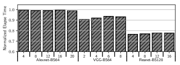
Figure 5: Normalized execution time of $A^{2}$DTWP with respect to baseline considering the Imagenet1000 data set. Training for Alexnet, VGG and Resnet considers up to 20, 8, and 16 epochs, respectively.

In terms of validation error, both $A^{2}$DTWP and baseline display very similar top-5 values at the end of each epoch. For example, for the case of VGG, the Floating Point 32-bit baseline approach displays a validation error of 88.04% after 2 training epochs while $A^{2}$DTWP achieves a validation error of 89.97% for the same epoch count, that is, an absolute difference of 1.93%. After 8 training epochs the absolute distance of top-5 validation errors between $A^{2}$DTWP and baseline is 0.71%. Top-5 validation error keeps decreasing in an analogous way for both baseline and $A^{2}$DTWP as training goes over more epochs, although $A^{2}$DTWP is significantly faster. Our evaluation indicates that $A^{2}$DTWP can effectively accelerate training while achieving the same validation error as the 32-bit FP baseline when considering ImageNet1000.

V-G $A^{2}DTWP$ Performance Profile

This section provides a detailed performance profile describing the effects of applying $A^{2}DTWP$ when training the VGG network model with batch size 64 on the x86 and POWER systems described in section IV-D. To highlight these effects we also show a performance profile of applying 32-bit Floating Point format during training. The main kernels involved in the training process and their corresponding average execution time in milliseconds are shown in Tables  II and III. Each kernel can be invoked multiple times by different network layers and it can be overlapped with other operations while processing a batch. Tables II and III display for all kernels the average execution time of their occurrences within a batch when run on the x86 and the POWER systems, respectively.

Results appearing in Table II show how time spent transferring data from the CPU to the GPU accelerators when applying $A^{2}DTWP$ on the x86 system, 52.27 ms, is significantly smaller than the cost of performing the same operation when using the 32-bit configuration, 153.93 ms. This constitutes a 2.94x execution time reduction that compensates the cost of the operations involved in the ADT routine, Bitpack and Bitunpack, and in the AWP algorithm, the $l^{2}$-norm computation. On POWER we observe a similar reduction of 3.20x in the time spent transferring data from the CPU to the GPUs when applying $A^{2}DTWP$. These reductions in terms of CPU to GPU data transfer time are due to a close to 3x reduction in terms of weights size enabled by $A^{2}DTWP$. The average execution time of operations where the $A^{2}DTWP$ technique plays no role remains very similar for the 32-bit Floating Point baseline and $A^{2}DTWP$ in both systems, as expected. Tables II and III indicate that performance gains achieved by $A^{2}DTWP$ are due to data motion reductions, which validates the usefulness of $A^{2}DTWP$.

Tables II and III also display the overhead associated with AWP and ADT in terms of milliseconds. The AWP algorithm spends most of its runtime computing the $l^{2}$-norm of the weights, which takes a total of 3.88 ms within a batch on the x86 system. On POWER, the cost of computing the $l^{2}$-norm of the weights is 0.93 ms. The other operations carried out by AWP have a negligible overhead. The two fundamental procedures of ADT are the Bitpack and Bitunpack routines, which take 19.71 and 4.51 ms to run within a single batch on the x86 system. For the case of POWER, Bitpack and Bitunpack take 10.51 and 1.11 ms, respectively. Overall, measurements displayed at Table II indicate that AWP and ADT constitute 1.05% and 6.60% of the total batch execution time, respectively, on x86. On the POWER system, AWP and ADT constitute 0.54% and 6.82% of the total batch execution time according to Table III. Figures  3 and  4 account for this overhead in the results they display.

TABLE II: Performance profiles of both the $A^{2}DTWP$ and the 32-bit Floating Point approaches expressed in milliseconds on the x86 system. We consider the VGG network model with batch size 64.

	32-bit FP	$\mathbf{A^{2}DTWP}$
Data Transfer CPU$\rightarrow$GPU	153.93	52.27
Data Transfer GPU$\rightarrow$CPU	68.51	73.55
Convolution	128.72	126.13
Fully-connected	33.51	34.17
Gradient update	54.39	52.86
AWP ($l^{2}$-norm)	N/A	3.88
ADT (Bitpack)	N/A	19.71
ADT (Bitunpack)	N/A	4.51

TABLE III: Performance profiles of both the $A^{2}DTWP$ and the 32-bit Floating Point approaches expressed in milliseconds on the POWER system. We consider the VGG network model with batch size 64.

	32-bit FP	$\mathbf{A^{2}DTWP}$
Data Transfer CPU$\rightarrow$GPU	39.12	12.21
Data Transfer GPU$\rightarrow$CPU	17.34	17.87
Convolution	69.78	71.21
Fully-connected	12.66	13.51
Gradient update	41.29	42.98
AWP ($l^{2}$-norm)	N/A	0.93
ADT (Bitpack)	N/A	10.51
ADT (Bitunpack)	N/A	1.11

VI Related work

A rich body of literature exists in describing the impact of using data representation formats smaller than the 32-bit Floating Point standard while training neural networks. Previous work provides theoretical analysis on the learning capability under limited-precision scenarios of simple networks [31]. In recent years, researchers have shown that fixed-precision arithmetic is well suited for deep neural networks training [32], particularly when combined with stochastic rounding [12]. New data representation formats targeting dynamic and low accuracy opportunities for deep learning have been proposed [13, 33]. While these approaches have a very large potential for reducing DNNs training costs, they do not target the data movement problem and, as such, they are orthogonal to the approach presented by this paper.

There is a methodology for training deep neural models using 16-bit FP numbers without modifying hyperparameters or losing network accuracy [18]. This previous approach avoids losing accuracy by keeping a 32-bit copy of weights, scaling the loss function to preserve small gradient updates, and using 16-bit arithmetic that accumulates into single-precision registers. While it also exploits the tolerance of DNN to data representation formats with less precision than the 32-bit FP standard, our goal is fundamentally different since we reduce data motion in the context of heterogeneous high-end architectures while this previous approach aims at reducing the computing and storage costs of DNN training. This approach can be combined with $A^{2}$DTWP by decompressing network weights to half-precision to reduce GPU computing time. This reduction would increase the impact of data motion in the overall performance, which imples that the benefits of $A^{2}$DTWP could be evern larger.

Other approaches exploit model parallelism instead of data-level parallelism to orchestrate parallel executions of deep learning workloads [34, 35]. If the different parallel instances of this model-level parallel scheme had different precision requirements, $A^{2}$DTWP would obtain very significant performance improvements.

Some previous approaches reduce DNNs storage and energy requirements to run inference on mobile devices [36] and achieve large graident compression ratios in the context of mobile device distributed trainign [37]. While these approaches achieve very large storage reductions and substantial speedups, they target mobile computing.

Asynchronous SGD [38] and its variants [39, 40] target the synchronization cost of SGD gradient updates. Other approaches either quantize gradients to ternary levels {-1, 0, 1} to reduce the overhead of gradient synchronization [41], or propose a family of algorithms allowing for lossy compression of gradients called Quantized SGD (QSGD) [42]. Techniques based on sparsifying gradient updates by removing the smallest gradients by absolute value [43] can also reduce SGD synchronization costs. While some of these approaches apply techniques based on small data representation formats to reduce the synchronization costs of SGD gradient updates, $A^{2}$DTWP targets the cost of sending DNNs weights to the GPU accelerators. Therefore, these approaches are orthogonal to $A^{2}$DTWP and can be combined with it to reduce as much as possible training communication cost. In particular, techniques targeting synchronization overhead of SGD gradient updates can be used to reduce GPU to CPU data transfer overhead while $A^{2}$DTWP targets CPU to GPU communication cost.

To the best of our knowledge, this paper is the first in accelerating the training of deep neural networks in multi-GPU high-end systems by reducing data motion.

VII Conclusion

This paper proposes $A^{2}DTWP$, which reduces data movement across heterogeneous environments composed of several GPUs and multicore CPU devices in the context of deep learning workloads. The $A^{2}DTWP$ framework is composed of the AWP algorithm and the ADT procedure. AWP is able to dynamically define the weights data representation format during training. This paper demonstrates that AWP is effective without any deterioration on the learning capacity of the neural network. To transform AWP decisions into real performance gains, we introduce the ADT procedure, which efficiently compresses network’s weights before sending them to the GPUs. This procedure exploits both thread- and SIMD-level parallelism. By combining AWP with ADT we are able to achieve a significant performance gain when training network models such as Alexnet, VGG or Resnet. Our experimental campaign considers different batch sizes and two different multi-GPU high-end systems.

This paper is the first in proposing a solution that relies on reduced numeric data formats to mitigate the cost of sending DNNs weights to different hardware devices during training. While our evaluation targets heterogeneous high-end systems composed of several GPUs and CPU multicore devices, techniques presented by this paper are easily generalizable to any context involving several hardware accelerators exchanging large amounts of data. Taking into account the prevalence of deep learning-specific accelerators in large production systems [9], the contributions of this paper are applicable to a wide range of scenarios involving different kinds of accelerators.

References

- [1] A. Krizhevsky, I. Sutskever, and G. E. Hinton, “Imagenet classification with deep convolutional neural networks,” 2012.
- [2] C. Szegedy, W. Liu, Y. Jia et al., “Going deeper with convolutions,” in Proc. of the IEEE Conf. on Computer Vision and Pattern Recognition, 2015, pp. 1–9.
- [3] G. Hinton, L. Deng, D. Yu et al., “Deep neural networks for acoustic modeling in speech recognition: The shared views of four research groups,” IEEE Signal Processing Magazine, vol. 29, no. 6, pp. 82–97, 2012.
- [4] Y. Wu, M. Schuster, Z. Chen et al., “Google’s neural machine translation system: Bridging the gap between human and machine translation,” arXiv preprint arXiv:1609.08144, 2016.
- [5] D. Ciregan, U. Meier, and J. Schmidhuber, “Multi-column deep neural networks for image classification,” in 2012 IEEE Conf on Computer Vision and Pattern Recognition, June 2012, pp. 3642–3649.
- [6] A. Krizhevsky, I. Sutskever, and G. E. Hinton, “ImageNet Classification with Deep Convolutional Neural Networks,” ser. NIPS’12, USA, 2012, pp. 1097–1105.
- [7] M. Abadi, P. Barham, J. Chen et al., “Tensorflow: A system for large-scale machine learning,” ser. OSDI’16, 2016, pp. 265–283.
- [8] P. A. Merolla, J. V. Arthur, R. Alvarez-Icaza et al., “A million spiking-neuron integrated circuit with a scalable communication network and interface,” Science, vol. 345, no. 6197, pp. 668–673, 2014.
- [9] N. P. Jouppi, C. Young, N. Patil et al., “In-datacenter performance analysis of a tensor processing unit,” ser. ISCA ’17, 2017, pp. 1–12.
- [10] T. Kurth, J. Zhang, N. Satish et al., “Deep learning at 15pf: Supervised and semi-supervised classification for scientific data,” ser. SC ’17, 2017, pp. 7:1–7:11.
- [11] Y. You, A. Buluc, and J. Demmel, “Scaling deep learning on gpu and knights landing clusters,” ser. SC ’17, 2017, pp. 9:1–9:12.
- [12] S. Gupta, A. Agrawal, K. Gopalakrishnan, and P. Narayanan, “Deep learning with limited numerical precision,” in Proc. of the 32nd International Conference on Machine Learning, ICML 2015, 2015, pp. 1737–1746.
- [13] U. Köster, T. Webb, X. Wang et al., “Flexpoint: An adaptive numerical format for efficient training of deep neural networks,” in Advances in Neural Information Processing Systems 30, 2017, pp. 1742–1752.
- [14] K. Simonyan and A. Zisserman, “Very deep convolutional networks for large-scale image recognition,” CoRR, vol. abs/1409.1556.
- [15] K. He, X. Zhang, S. Ren, and J. Sun, “Deep residual learning for image recognition,” in 2016 IEEE Conference on Computer Vision and Pattern Recognition (CVPR), June 2016, pp. 770–778.
- [16] J. Deng, W. Dong, R. Socher et al., “ImageNet: A Large-Scale Hierarchical Image Database,” in CVPR09.
- [17] L. Bottou and O. Bousquet, “The tradeoffs of large scale learning,” in Advances in Neural Information Processing Systems, 2008.
- [18] P. Micikevicius, S. Narang, J. Alben et al., “Mixed precision training,” Seventh International Conference on Learning Representations (ICLR), 2018.
- [19] A. F. Murray and P. J. Edwards, “Enhanced mlp performance and fault tolerance resulting from synaptic weight noise during training,” IEEE Transactions on Neural Networks, vol. 5, no. 5, 1994.
- [20] C. M. Bishop, “Training with noise is equivalent to tikhonov regularization,” Neural Comput., vol. 7, no. 1, pp. 108–116, 1995.
- [21] K. Audhkhasi, O. Osoba, and B. Kosko, “Noise benefits in backpropagation and deep bidirectional pre-training,” in IJCNN 2013, 2013, pp. 1–8.
- [22] L. Dagum and R. Menon, “Openmp: An industry-standard api for shared-memory programming,” IEEE Comput. Sci. Eng., pp. 46–55, Jan. 1998.
- [23] C. Lomont, “Introduction to intel advanced vector extensions. intel white paper,” 2011.
- [24] L. Gwennap, “AltiVec Vectorizes PowerPC,” Microprocessors Report, vol. 12, no. 6, pp. 1–5, May 1998.
- [25] “Ieee standard for floating point arithmetic,” IEEE Std 754-2008, pp. 1–70, 2008.
- [26] A. Krizhevsky, “One weird trick for parallelizing convolutional neural networks,” CoRR, vol. abs/1404.5997.
- [27] H. Seo, Z. Liu, J. Großschädl, and H. Kim, “Efficient arithmetic on arm-neon and its application for high-speed rsa implementation.” IACR Cryptology ePrint Archive, vol. 2015, p. 465, 2015.
- [28] J. Nickolls, I. Buck, M. Garland, and K. Skadron, “Scalable parallel programming with cuda,” Queue, vol. 6, no. 2, pp. 40–53, Mar. 2008.
- [29] N. Qian, “On the momentum term in gradient descent learning algorithms,” Neural Networks, vol. 12, no. 1, pp. 145 – 151, 1999.
- [30] N. Corp. (2016) Nvlink fabric.
- [31] J. L. Holi and J. N. Hwang, “Finite precision error analysis of neural network hardware implementations,” IEEE Transactions on Computers, vol. 42, no. 3, pp. 281–290, Mar 1993.
- [32] M. Courbariaux, Y. Bengio, and J. David, “Low precision arithmetic for deep learning,” CoRR, vol. abs/1412.7024, 2014.
- [33] D. D. Kalamkar, D. Mudigere, N. Mellempudi et al., “A study of BFLOAT16 for deep learning training,” CoRR, vol. abs/1905.12322, 2019.
- [34] A. Coates, B. Huval, T. Wang et al., “Deep learning with cots hpc systems,” ser. ICML’13, 2013, pp. III–1337–III–1345.
- [35] Q. V. Le, R. Monga, M. Devin et al., “Building high-level features using large scale unsupervised learning,” CoRR, vol. abs/1112.6209, 2011.
- [36] S. Han, X. Liu, H. Mao et al., “EIE: efficient inference engine on compressed deep neural network,” CoRR, vol. abs/1602.01528, 2016.
- [37] Y. Lin, S. Han, H. Mao, Y. Wang, and W. J. Dally, “Deep gradient compression: Reducing the communication bandwidth for distributed training,” CoRR, vol. abs/1712.01887, 2017.
- [38] J. Dean, G. S. Corrado, R. Monga et al., “Large scale distributed deep networks,” in NIPS, 2012.
- [39] F. Niu, B. Recht, C. Re, and S. J. Wright, “Hogwild!: A lock-free approach to parallelizing stochastic gradient descent,” ser. NIPS’11, 2011, pp. 693–701.
- [40] S. Zhang, A. Choromanska, and Y. LeCun, “Deep learning with elastic averaging SGD,” CoRR, vol. abs/1412.6651, 2014.
- [41] W. Wen, C. Xu, F. Yan et al., “Terngrad: Ternary gradients to reduce communication in distributed deep learning,” CoRR, vol. abs/1705.07878, 2017.
- [42] D. Alistarh, J. Li, R. Tomioka, and M. Vojnovic, “QSGD: randomized quantization for communication-optimal stochastic gradient descent,” CoRR, vol. abs/1610.02132, 2016.
- [43] A. F. Aji and K. Heafield, “Sparse communication for distributed gradient descent,” CoRR, vol. abs/1704.05021, 2017.