Viscoelastic multiscaling in immersed networks

Abstract

Rheological responses are the most relevant features to describe soft matter. So far, such constitutive relations are still not well understood in terms of small scale properties, although this knowledge would help the design of synthetic and bio-materials. Here, we investigate, computational and analytically, how mesoscopic-scale interactions influence the macroscopic behavior of viscoelastic materials. We design a coarse-grained approach where the local elastic and viscous contributions can be controlled. Applying molecular dynamics simulations, we mimic real indentation assays. When elastic forces are dominant, our model reproduces the hertzian behavior. However, when friction increases, it restores the Standard Linear Solid model. We show how the response parameters depend on the microscopic elastic and viscous contributions. Moreover, our findings also suggest that the relaxation times, obtained in relaxation and oscillatory experiments, obey a universal behavior in viscoelastic materials.

One big challenge in science and engineering is the so-called multiscale modeling, namely, how constitutive relations of a material depend on its smaller scale interaction and composition Yip2013 ; White2009 . Such emergence problem, as described by P. W. Anderson Anderson1972 , is even more remarkable in soft matter, where mesoscopic structures combine the atomistic and macroscopic frameworks and are responsible to the material elasticity and viscosity Doi2013 ; Praprotnik2008 . In fact, the link among features of different scales forming the matter is highly nontrivial and subjected to intense research Qu2011 . The seminal work of H. Hertz about mechanical contacts, for instance, is still used nowadays to measure elastic properties of materials by analyzing how samples are deformed under applied stresses Hertz1881 . Although it is one of the most used models to investigate the stiffness of a material, it fails to relate the macroscopic behavior with its inner parts. Besides, well-known analytical approaches such as the Maxwell, Kelvin-Voigt, and Standard Linear Solid models apply circuit analogies to propose a simple manner of how elastic and viscous terms mix up in viscoelastic materials Lakes2017 . Again, these rheological models neglect any downscaling analysis.

Currently, many sophisticated methods have been developed to study the viscoelasticity of materials. Nanoindentation experiments, for instance, such as those with Atomic Force Microscopy, are extensively applied to investigate the mechanical properties at micrometer scale. Besides condensed matter, such technique has also been used to investigate soft materials Lin2008 ; Radmacher1997 ; Rebelo2013 . The way the sample responses to external stresses depends on its elastic and viscous terms. However, the complex structure and composition in soft matter systems make it challenging to investigate accurately the distribution of applied stresses through their interior. Many soft matter systems hold large colloidal aggregations or long (linear or cross-linked) polymeric chains, which have an essential mechanical role Doi2013 . In living cells, for instance, the cytoskeleton and the cytoplasmic fluid are constantly exchanging momentum with the extracellular surroundings Gupta2015 ; Moeendarbary2013 . The knowledge of why these organelles influence the cell stiffness differently in healthy and sick cells, may lead to treatments for several diseases Sousa2020 .

To investigate the link between mesoscopic and macroscopic features, we employ a molecular coarse-grained approach to reproduce rheological behavior of soft matter. We design a viscoelastic material composed of a particle-spring network immersed in a viscous medium so that the contribution of elastic and viscous interactions can be controlled at the mesoscopic level. This immersed network model is compatible with suspended polymer chains, colloidal aggregations, and other load-bearing structures as commonly found in soft materials Doi2013 . Although real materials unlikely present purely quadratic potentials, for small deviations, molecular interactions displaying a potential well can be described appropriately by a spring-like interaction. For instance, the equivalent spring constant of the Lennard-Jones interatomic potential can be calculated as $72\epsilon_{0}/\ell_{0}^{2}$, where $\epsilon_{0}$ is the height of the potential well and $\ell_{0}$ the equilibrium distance between molecules Kleppner2014 . Moreover, the computational model we develop here is easily changed to support a more realistic potential in order to study more complex materials. We also consider the spring network as a regular lattice. Although complex structures may influence rheological properties of a material, simple geometries have been successfully applied to a large number of problems in mesoscopic models of condensed Oliveira2012 ; Moreira2012 and soft materials Oliveira2014 ; Alves2016 ; Dias2012 .

Our computational model consists of $N$ spherical particles of diameter $\sigma$ and mass $m$ arranged in a face-centered cubic (FCC) lattice with a height given by $H$ and a bottom and top plane given by $20\sigma\times 20\sigma sin(\pi/3)$. Every particle interacts with its 12 nearest neighbors by a spring potential. This elastic network is immersed in a medium of viscosity $\mu$. Viscous effects are taken into account by considering friction between the particles and the medium. The network is indented by a hard sphere of diameter $\sigma_{s}$, as shown in Fig. 1. This spherical indenter moves down with constant speed until a maximum indentation depth, $\delta_{0}$, is achieved. To avoid non-linearities, we consider $\delta_{0}=\sigma$, i.e., the maximum indentation is equal to the thickness of one layer of particles. Once in contact, the indenter applies a stress onto the particles. The bottom layer of the network is in contact to a hard substrate, where particles cannot move down but are free to slide horizontally.

The equation of motion of the $i_{th}$ particle is given by the following Langevin-like equation Langevin1908 ; Langevin

$$m\frac{d^{2}\vec{r}_{i}}{dt^{2}}=-\gamma\vec{v}_{i}-\nabla U_{i},$$ (1)

where $\vec{r}_{i}$ and $\vec{v}_{i}$ are the position and velocity vectors of particle $i$, respectively. The term $\gamma\vec{v}_{i}$, known as Stoke’s law, describes the drag force acting on spherical bodies, where the coefficient of friction is given by $\gamma=3\pi\sigma\mu$ Batchelor1967 . The potential $U_{i}$ of particle $i$ due to the neighboring particles and the indenter is given by

$$U_{i}=\sum_{j}\frac{k_{ij}(r_{ij}-\ell)^{2}}{2}+\epsilon\left(\frac{\sigma}{r_{is}-(\sigma_{s}-\sigma)/2}\right)^{\alpha},$$ (2)

where $r_{ij}=|\vec{r}_{i}-\vec{r}_{j}|$ is the distance and $\ell$ the equilibrium distance between the centers of neighboring particles $i$ and $j$. $k_{ij}$ is the spring constant of the bond between these two particles. The last term of Eq. 2 applies only to surface particles, when they are in contact with the indenter. $r_{is}=|\vec{r}_{i}-\vec{r}_{s}|$ is the distance between the center of particle $i$ and the center of the indenter, $\epsilon$ is a constant of energy, and $\alpha$ regulates the hardness of the indenter. The particles and the indenter exclusively interact through this hard-sphere potential with a high value of $\alpha$. See in Ref. param the constants used in this work.

We solve the equations of motion in (1) through molecular dynamics simulations with a time integration done with the Velocity Verlet algorithm, and periodic boundary conditions applied to the horizontal plane Rapaport2004 ; Araujo2017 . The contact force $F$ is the sum of all collisions on the indenter, computed at each time as the indenter slowly presses down the sample. $F$ increases with the indentation depth, $\delta$, since more collisions occur on the indenter. These collisions cause a fluctuation in $F$, but an equilibrium state is reached in around $10^{5}$ time steps. After equilibrium, we perform an additional $2\times 10^{5}$ time steps to average the quantities of interest.

Before viscoelastic materials, we explore the elasticity in networks without local friction ($\gamma=0$). Initially, we study homogenous networks, where all bonds have the same spring constant, $k_{ij}=k$, and later we investigate the role of heterogeneities of local elasticity in the global stiffness. For simplicity, we consider heterogeneous networks made of only two types of bonds with spring constants given by $k_{1}$ and $k_{2}$, respectively. Moreover, this binary network is built in two fashions depending on the distribution of $k_{1}$ and $k_{2}$, namely, the double-layered and the binary random network. In the first, two homogenous networks, with spring constants given by $k_{1}$ and $k_{2}$, respectively, are deposited one on the top of the other (see the inset in Fig. 2(a)). In the second, $k_{ij}$ is randomly assigned to $k_{1}$ or $k_{2}$ according to probabilities $\phi_{1}$ and $\phi_{2}$, respectively (see the inset in Fig. 2(b)). In both cases, $\phi_{1}$ and $\phi_{2}$ also stand to the fraction of each bond and $\phi_{1}+\phi_{2}=1$. For the limit cases of $\phi_{1}=0$ and $\phi_{1}=1$, both the double-layered and the binary random networks become homogeneous with spring constant $k_{2}$ and $k_{1}$, respectively.

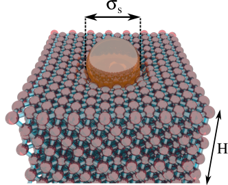
Figure 1: Particle-spring network arranged in an FCC (face-centered cubic) lattice with height $H$ and immersed in a viscous medium (not shown in the figure). Particles are bonded to their 12 nearest neighbors. A spherical indenter of diameter $\sigma_{s}$ is used to press down the top surface of the network.

The distribution of stress into an elastic sample, due to an indentation $\delta$, can be tricky Sneddon1965 , however the force experienced by a spherical indenter is well described by the Hertz model

$$F_{H}=\frac{8\sqrt{2}}{9}E\sqrt{\sigma_{s}}\delta^{3/2},$$ (3)

where $E$ is the effective elastic modulus of the material Dimitriadis2002 (see Fig. S1 in the Supplementary Material). The contact forces computed in elastic networks perfectly agree with the Hertz model, where $E$ can be obtained by fitting the data with Eq. 3. The results for homogeneous elastic networks are shown in Fig. S2 in the Supplementary Material for different values of $k$. As expected for this simple network, the effective modulus of elasticity scales linearly with $k$. In addition, $E$ is proportional to the sample height in the form $E\propto H^{-\zeta}$, where $\zeta$ depends on the indenter geometry. Spherical and flat indenters, for instance, give $\zeta=1/3$ and 1, respectively. In fact, in the latter case, $E$ represents the Young’s modulus of the material and can be found analytically with springs in series, while in the other case, $E$ seems to take into account, besides Young’s modulus, the shear modulus of the material.

The effective elastic modulus as a function of $\phi_{1}$ is shown in Fig. 2(a), for double-layered networks, and in Fig. 2(b), for binary random networks, for $k_{2}=500$ and different values of $k_{1}$. $E$ decreases with $\phi_{1}$ for $k_{1}<k_{2}$, but increases with $\phi_{1}$ for $k_{1}>k_{2}$, regardless the distribution of $k_{1}$ and $k_{2}$. In double-layered networks, $E$ is fitted by the cubic function $E=570.75+a\phi+b\phi^{2}+c\phi^{3}$, shown in colored solid lines. On the other hand, when $k_{1}$ and $k_{2}$ are randomly distributed over the network, $E$ changes according to the straight line $E=570.75+d\phi$, shown in colored solid lines. The constants $a$, $b$, $c$, and $d$ depend on $k_{1}$. Interestingly, the random distribution of local stiffness vanishes those polynomial higher order found in (a).

In order to study the contribution of viscous effects ($\gamma>0$) in the macroscopic rheological behavior, we perform relaxation and oscillatory assays in homogenous viscoelastic networks. In relaxation experiments, the indenter is initially located above the network and moving down into the top surface. Before touching the sample, the force is zero. When the indenter touches the surface particles, at time $t_{1}=0$, the force rises until the maximum indentation depth, $\delta_{0}$, is achieved, at $t_{3}$. Figure 3 shows the time evolution of the normalized contact force, $f$, for $k=500$ and several values of $\gamma$. The loading time, $\tau_{l}=t_{3}-t_{1}$, is the time the indenter pushes the sample. After reaching $\delta_{0}$, the indenter stops moving, but the sample particles may continue to move subjected to friction (the dwell stage). For elastic $\gamma=0$, the particles immediately rearrange themself to an equilibrium state and thus the force becomes nearly constant, except for some noise due to the perpetual undamped movement of the particles. On the other hand, in viscoelastic networks, this noise quickly vanishes while the force decreases continuously to the value of the undamped case, at $t_{4}$, since particles need time to relax into the equilibrium state. For long times, networks with the same elastic properties experience the same contact force, regardless of the viscous contribution.

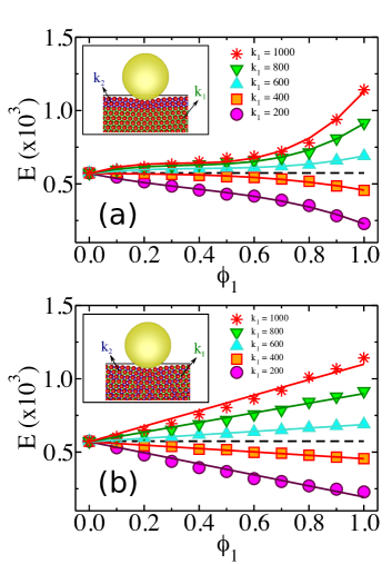
Figure 2: The effective modulus of elasticity, $E$, as a function of the fraction of $k_{1}$-bonds in heterogeneous elastic networks, $\phi_{1}$, for $k_{2}=500$ and several values of $k_{1}$. The double-layered network is in shown in (a) while the binary random network in (b). The inset of each graph shows how $k_{1}$ and $k_{2}$ are distributed in the network. The black dashed lines in each graph represent the elastic modulus of homogeneous networks, for $k_{1}=k_{2}=500$, with $E=570.75$. Cubic functions and straight lines, shown in colored solid lines, are used to fit each set of points in (a) and (b), respectively.

Our numerical results are compatible with the Standard Linear Solid (SLS) model composed of a Maxwell material (i.e., a spring of elastic modulus $E_{0}$ in series with a dashpot of viscosity $\eta$) in parallel to another spring of elastic modulus $E_{\infty}$, see Fig. 3. Such analytical model successfully describes rheological behaviors of a large number of soft materials, such as polymers Plaseied2008 , soft gels Okamoto2011 , and living cells Peeters2005 ; Koay2003 . The relaxation function of this model is know as $R(t)=E_{\infty}+E_{0}e^{-t/\tau}$, where the relaxation time is given by $\tau=\eta/E_{0}$. Initially, the effective modulus of elasticity is given by the sum of $E_{\infty}$ and $E_{0}$, but, for long times, the influence of $E_{0}$ vanishes, leaving $E_{\infty}$ to dominate the elasticity of the material, regardless of the relaxation time. Notice that, $E_{\infty}$ corresponds to the elastic modulus computed in elastic networks. The analytical force curves in the SLS model with a spherical indenter, $f(t)$, can be obtained separately in the loading, $f_{l}(t)$, and dwell stages, $f_{d}(t)$, as follows

$$f_{l}(t) = a_{1}t^{3/2}+a_{2}\sqrt{t}+a_{3}\,erf\left(\sqrt{\frac{t}{\tau}}\right)e^{-t/\tau},\hskip 2.84544ptt\leq\tau_{l},$$

$$f_{d}(t) = a_{4}+a_{5}e^{-(t-\tau_{l})/\tau}+a_{6}e^{-t/\tau},\hskip 19.91684ptt\geq\tau_{l},$$ (4)

where $erf(t)$ is the error function and the constants are given by

$$a_{1} = \frac{E_{\infty}}{\tau_{l}^{3/2}},\,\,\,a_{2}=\frac{3}{2}\frac{\tau}{\tau_{l}^{3/2}}E_{0},\,\,\,a_{3}=-\frac{3}{4}\sqrt{\pi}E_{0}\left(\frac{\tau}{\tau_{l}}\right)^{3/2},$$

$$a_{4} = E_{\infty},\,\,\,a_{5}=\frac{3}{2}\frac{\tau}{\tau_{l}}E_{0},\,\,\,a_{6}=a_{3}\,erf\left(\sqrt{\frac{\tau_{l}}{\tau}}\right).$$

See more details in Section I of the Supplementary Material.

Combining our numerical results with Eqs. 4 allows us to find the relations between macroscopic ($\tau$ and $E_{0}$) and microscopic parameters ($k$ and $\gamma$) in viscoelastic networks. As shown for elastic networks, $E_{\infty}$ increases linearly with $k$ and does not depend on $\gamma$. However, $\tau$ decreases with $k$ and increases with $\gamma$ (see Fig. 4(a)). On the other hand, $E_{0}$ increases with $k$ but decreases with the local dissipation (see Fig. 4(b)).

In oscillatory experiments, instead of stoping the indenter after the maximum indentation is achieved, a sinusoidal strain is imposed with the indentation depth following the function, $\delta(t)=\delta_{0}+\delta_{a}sin(\omega t)$, where $\delta_{a}$ ($\delta_{a}=\sigma$) is the amplitude and $\omega$ the angular frequency of oscillation. The response force $F$ also presents a periodic behavior but with a time delay that depends on viscoelastic properties, $F=F_{0}+F_{a}sin(\omega t+\lambda)$, where $F_{0}$ is the force at $\delta_{0}$, $F_{a}$ is the amplitude of the force and $\lambda$ is the phase lag between force and indentation. Figure S3(a) and (b), in the Supplementary Material, show $\delta(t)$ and $F(t)$, respectively, for a sample with $k=500$ and three values of $\gamma$. The phase lag vanishes for $\gamma=0$, as it is expected for elastic materials, but increases with $\gamma$, for viscoelastic materials.

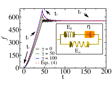
Figure 3: Relaxation experiments in viscoelastic networks, for $k=500$ and different values of $\gamma$. The contact force increases in the loading stage and decreases in the dwell stage. The force is normalized by geometric constants (see Eq. 4 in the Supplementary Material). Our numerical results are compatible with the Standard Linear Solid (SLS) model given in Eqs. 4. A schematic illustration of the SLS model is shown in the inset, with a dashpot of viscosity $\eta$ and two springs of elastic moduli $E_{0}$ and $E_{\infty}$.

The tangent of $\lambda$, defined as the ratio between the loss modulus, $G^{{}^{\prime}}=\frac{\delta_{a}}{F_{a}}sin(\lambda)$, and the storage modulus, $G^{{}^{\prime\prime}}=\frac{\delta_{a}}{F_{a}}cos(\lambda)$, represents a quantitative way to define the fluidity of viscoelastic materials, i.e., $\tan(\lambda)<1$ leads to solid-like materials while $\tan(\lambda)>1$ to fluid-like materials. High values of $\omega$ favor the fluidity of the material, as shown in panel of Fig. 5 for several values of $\gamma$. Figure S3(c) and (d), in the Supplementary Material, shows color maps of $\tan(\lambda)$ for more values of $k$ and $\gamma$. We only observe viscoelastic solids in all cases of $k$ and $\gamma$ considered in this work. Fluid-like behavior should be observed for very high values of $\omega$, which requires a time step too small compared to the time of the experiment. Moreover, viscoelastic materials may present different relaxation times regarding of how the sample is deformed. In this work, we obtained $\tau$ and $\tau_{o}$ in relaxation and oscillatory conditions, respectively. Standard Linear Solids under oscillatory strain leads to the following behavior Lakes2017

$$\tan(\lambda)=A\frac{\omega\tau_{o}}{1+\omega^{2}\tau_{o}^{2}},$$ (5)

which is used to fit those numerical data in Fig. 5 in order to obtain $\tau_{o}$, where $A$ is a constant of the material. The main graph in Fig. 5 shows that $\tau$ and $\tau_{o}$ depend on each other by the following exponential relation, $\tau=0.466(e^{0.08\tau_{o}}-1)$. Each point in the graph of Fig. 5(b) represents a different material, with different $k$ and $\gamma$, but they all collapse on that relation, suggesting some kind of universal behavior.

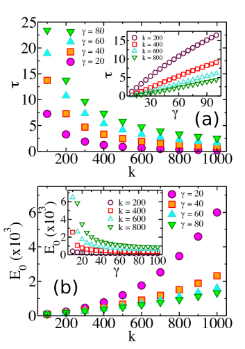
Figure 4: The macroscopic properties $\tau$ and $E_{0}$, in (a) and (b), respectively, as a function of microscopic parameters, $k$ and $\gamma$, in viscoelastic networks under relaxation assays.

In conclusion, we studied macroscopic rheological behaviors in viscoelastic soft materials in terms of their microscopic elastic and viscous constituents. Different indentation experiments were performed to investigated how the local stiffness and the coefficient of friction induce different macroscopic behaviors. Elastic networks recovers the Hertz model for mechanical contact, where the effective modulus of elasticity, $E$, is obtained. In homogeneous elastic networks, we found that $E\propto H^{-\zeta}$, where $H$ is the network height and the exponent depends on the indenter geometry. For spherical and flat indenters, for instance, $\zeta=1/3$ and $\zeta=1$, respectively. Heterogeneous elastic networks, for simplicity, are assumed to be binary networks, where each bond holds one of only two possible values, $k_{1}$ or $k_{2}$. When $k_{1}$ and $k_{2}$ are separated forming layers, $E$ follows a cubic function with $\phi_{1}$, however, when $k_{1}$ and $k_{2}$ are randomly distributed, the higher order terms vanish and $E$ changes linearly with $\phi_{1}$. Viscoelastic networks are compatible with the analytical Standard Linear Solid (SLS) model, which is described by two elastic moduli, $E_{0}$ and $E_{\infty}$, and a relaxation time, $\tau$. Therefore, our work applies to all those materials that can be described by the Hertz and SLS models, such as polymers, gels and living cells. In oscillatory experiments, we also computed the phase lag between force and indentation, $\lambda$, and the relaxation time, $\tau_{o}$. We showed how all these macroscopic properties ($E_{0}$, $E_{\infty}$, $\tau$, $\lambda$, and $\tau_{o}$) depend on the microscopic parameters. In addition, the interplay between different relaxation times, $\tau$ and $\tau_{0}$, obtained in relaxation and oscillatory experiments, follows an exponential behavior, regardless of the mesoscopic interactions. All viscoelastic networks simulated here collapsed on this curve, suggesting a universal behavior in viscoelastic materials.

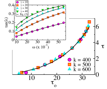
Figure 5: In oscillatory experiments, the tangent of the phase lag, $\lambda$, as a function of $\omega$, is shown in the panel for $k=500$ and different values of $\gamma$. Our results recover in a good agreement the behavior of $\tan(\lambda)$ given in Eq. 5, where the relaxation time in oscillatory experiments, $\tau_{o}$, is obtained. The relaxation times, $\tau$ and $\tau_{o}$, obtained in different experiments of deformation, depend on each other as follows, $\tau=0.466(e^{0.08\tau_{o}}-1)$ (shown in black solid line), regardless of $k$ and $\gamma$, as shown in the main graph.

- (1) S. Yip and M. P. Short, Multiscale materials modelling at the mesoscale, Nature Mater. 12, 774 (2013).
- (2) R. J. White, G. C. Y. Peng, and S. S. Demir, Multiscale modeling of biomedical, biological, and behavioral systems (Part 1) [Introduction to the special issue], IEEE Eng. Med Biol. Mag. 28 12 (2009).
- (3) P. W. Anderson, More is different, Science 177, 393 (1972).
- (4) Masao Doi, Soft Matter Physics (Oxford University Press, 2013).
- (5) M. Praprotnik, L. D. Site, and K. Kremer, Multiscale Simulation of Soft Matter: From Scale Bridging to Adaptive Resolution, Annu. Rev. Phys. Chem. 59, 545 (2008).
- (6) Z. Qu, A. Garfinkel, J. N. Weiss, and M. Nivala, Multi-scale modeling in biology: How to bridge the gaps between scales?, Prog. Biophys. Mol. Biol. 107, 21 (2011).
- (7) H. Hertz, Über die Berührung fester elastischer Körper, J. Reine Angew Mathematik 95, 156 (1881).
- (8) R. S. Lakes, Viscoelastic Solids (CRC Press, 2017).
- (9) D. C. Lin and F. Horkay, Nanomechanics of polymer gels and biological tissues: A critical review of analytical approaches in the Hertzian regime and beyond, Soft Matter 4, 669 (2008).
- (10) M. Radmacher, Measuring the elastic properties of biological samples with the AFM, IEEE Eng. Med. Biol. Mag. 16, 47 (1997).
- (11) L. M. Rebelo, J. S. de Sousa, J. Mendes Filho, and M. Radmacher, Comparison of the viscoelastic properties of cells from different kidney cancer phenotypes measured with atomic force microscopy, Nanotech. 24, 055102 (2013).
- (12) M. Gupta, B. R. Sarangi, J. Deschamps, Y. Nematbakhsh, A. Callan-Jones, F. Margadant, R.-M. Mège, C. T. Lim, R. Voituriez, and B. Ladoux, Nature Commun. 6, 7525 (2015).
- (13) E. Moeendarbary, L. Valon, M. Fritzsche, A. R. Harris, D. A. Moulding, A. J. Thrasher, E. Stride, L. Mahadevan, and G. T. Charras, Nature Mater. 12, 253 (2013).
- (14) J. S. de Sousa, R. S. Freire, F. D. Sousa, M. Radmacher, A. F. B. Silva, M. V. Ramos, A. C. O. Monteiro-Moreira, F. P. Mesquita, M. E. A. Moraes, R. C. Montenegro, and C. L. N. Oliveira, Double power-law viscoelastic relaxation of living cells encodes motility trends, Sci. Rep. 10, 4749 (2020).
- (15) D. Kleppner and R. Kolenkow, An Introduction to Mechanics - second edition (Cambridge University Press, 2014).
- (16) C. L. N. Oliveira, A. P. Vieira, H. J. Herrmann, and J. S. Andrade, Jr., Subcritical fatigue in fuse networks, Europhys. Lett. 100, 36006 (2012).
- (17) A. A. Moreira, C. L. N. Oliveira, A. Hansen, N. A. M. Araújo, H. J. Herrmann, and J. S. Andrade, Jr., Fracturing Highly Disordered Materials, Phy. Rev. Lett. 109, 255701 (2012).
- (18) C. L. N. Oliveira, J. H. T. Bates, and B. Suki, A network model of correlated growth of tissue stiffening in pulmonary fibrosis, New J. Phys. 16, 065022 (2014).
- (19) C. Alves, A. D. Araújo, C. L. N. Oliveira, J. Imsirovic, E. Bartolák-Suki, J. S. Andrade, and B. Suki, Homeostatic maintenance via degradation and repair of elastic fibers under tension, Sci. Rep. 6, 27474 (2016).
- (20) C. S. Dias, N. A. M. Araújo, and M. M. Telo da Gama, Nonequilibrium growth of patchy-colloid networks on substrates, Phys. Rev. E 87, 032308 (2012).
- (21) P. Langevin, Sur la théorie du mouvement brownien, Comptes Rendue Acad. Sci. (Paris) 146, 530 (1908).
- (22) Although similar, it is not exactly the Langevin equation since the random forces applied to the particles are not due to the molecules of the medium, but, instead, to other particles in the medium.
- (23) G. K. Batchelor, An Introduction to Fluid Dynamics (Cambridge University Press, 1967).
- (24) The following are some values used in this work. Network parameters: ; ; ; , except in Fig S2(b) where is changed; and , except in Fig. S1 where is changed. In the particle-indenter interaction: and . The indenter radius is . The time step in the Velocity Verlet algorithm is 0.001.
- (25) D. C. Rapaport, The Art of Molecular Dynamics Simulation - second edition (Cambridge University Press, 2004)
- (26) J. L. B. de Araújo, F. F. Munarin, G. A. Farias, F. M. Peeters, and W. P. Ferreira, Structure and reentrant percolation in an inverse patchy colloidal system, Phys. Rev. E 95, 062606 (2017).
- (27) I. N. Sneddon, The relation between load and penetration in the axisymmetric Boussinesq problem for a punch of arbitrary profile, Int. J. Eng. Sci. 3, 47 (1965).
- (28) E. K. Dimitriadis, F. Horkay, J. Maresca, B. Kashar, and R. S. Chadwick, Determination of elastic moduli of thin layers of soft material using the atomic force microscope, Biophys. J. 82, 2798 (2002).
- (29) A. Plaseied and A. Fatemi, Deformation response and constitutive modeling of vinyl ester polymer including strain rate and temperature effects, J. Mater. Sci. 43, 1191 (2008).
- (30) R. J. Okamoto, E. H. Clayton, and P. V. Bayly, Viscoelastic properties of soft gels: comparison of magnetic resonance elastography and dynamic shear testing in the shear wave regime, Phys. Med. Biol. 56, 6379 (2011).
- (31) E. A. G. Peeters, C. W. J. Oomens, C. V. C. Bouten, D. L. Bader, and F. P. T. Baaijens, Viscoelastic properties of single attached cells under compression, J. Biomech. Eng. 127, 237 (2005).
- (32) E. J. Koay, A. C. Shieh, and K. A. Athanasiou, Creep indentation of single cells, J. Biomech. Eng. 125, 334 (2003).