Newton Hard Thresholding Pursuit for Sparse LCP via A New Merit Function

Abstract

Solutions to the linear complementarity problem (LCP) are naturally sparse in many applications such as bimatrix games and portfolio section problems. Despite that it gives rise to the hardness, sparsity makes optimization faster and enables relatively large scale computation. Motivated by this, we take the sparse LCP into consideration, investigating the existence and boundedness of its solution set as well as introducing a new merit function, which allows us to convert the problem into a sparsity constrained optimization. The function turns out to be continuously differentiable and twice continuously differentiable for some chosen parameters. Interestingly, it is also convex if the involved matrix is positive semidefinite. We then explore the relationship between the solution set to the sparse LCP and stationary points of the sparsity constrained optimization. Finally, Newton hard thresholding pursuit is adopted to solve the sparsity constrained model. Numerical experiments demonstrate that the problem can be efficiently solved through the new merit function.

90C33, 90C2, 90C30

1 Introduction

The linear complementarity problem (LCP) aims at finding a vector $x\in{\mathbb{R}}^{n}$ such that

(1) $$x\in{\texttt{sol}(M,q)}:=\{x\in{\mathbb{R}}^{n}:~{}x\geq 0,\ Mx+q\geq 0,\ \langle x,Mx+q\rangle=0\},$$

where $M\in{\mathbb{R}}^{n\times n}$ and $q\in{\mathbb{R}}^{n}$. Here, $x\geq 0$ means that each element of $x$ is nonnegative. Linear complementarity problems have extensive applications in economics and engineering such as Nash equilibrium problems, traffic equilibrium problems, contact mechanics problems and option pricing, to name a few. More applications can be found in [5, 6, 7] and the references therein. Among them, there is an important class trying to seek for a solution where most of its elements are zeros, namely, a sparse solution. For example, players in bimatrix games are willing to choose a small portion of reasonable strategies from a set of pure strategies to save their computational time. In the portfolio selection problem, most investors are only interested in a ‘small’ portfolio from a group of assets, see more details in [5, 38, 34]. Mathematically, these examples can be characterized as the following sparse LCP

(2) $$x\in{\texttt{sol}(M,q)}\cap S\ \ \ \ {\rm with}\ \ \ \ S:=\{x\in{\mathbb{R}}^{n}:~{}\|x\|_{0}\leq s\},$$

where $\|x\|_{0}$ is the zero norm of $x$, which counts the number of nonzero elements of $x$, and $s\ll n$ is a positive integer. Note that $\|\cdot\|_{0}$ is not a norm in the sense of the standard definition. In order to address the LCP, a commonly used approach is to convert the problem into an unconstrained minimization problem through the NCP (nonlinear complementarity problem) functions. A function $\psi:{\mathbb{R}}\times{\mathbb{R}}\rightarrow{\mathbb{R}}$ is called an NCP function if it satisfies

(3) $$\psi(a,b)=0\ \ \Longleftrightarrow\ \ a\geq 0,\ \ b\geq 0,\ \ ab=0.$$

In this paper, we introduce a new function $\phi_{r}:{\mathbb{R}}\times{\mathbb{R}}\rightarrow{\mathbb{R}}$ defined by

(4) $$\phi_{r}(a,b):=\frac{1}{r}\Big{[}a_{+}^{r}b_{+}^{r}+(-a)_{+}^{r}+(-b)_{+}^{r}\Big{]}:=\frac{1}{r}\Big{[}a_{+}^{r}b_{+}^{r}+|a_{-}|^{r}+|b_{-}|^{r}\Big{]}.$$

where $r>0$ is a given parameter, $a_{+}:=\max\{a,0\}$ and $a_{-}:=\min\{a,0\}$. It is easy to see that $\phi_{r}$ is indeed an NCP function for any given $r>0$. However, through this paper, we only focus on choices of $r\geq 2$. Because this new function is proven to be continuously differentiable everywhere for any $r\geq 2$ and twice continuously differentiable for any $r>2$, see Proposition 2.2. When it comes to model (1), we construct a new merit function $f_{r}$ through $\phi_{r}$ as

$$f_{r}(x) := \sum_{i=1}^{n}\phi_{r}(x_{i},M_{i}x+q_{i})$$

$$= \frac{1}{r}\Big{[}\left\langle x_{+}^{r},(Mx+q)_{+}^{r}\right\rangle+\|x_{-}\|_{r}^{r}+\|(Mx+q)_{-}\|_{r}^{r}\Big{]},$$

where $\|x\|_{r}^{r}:=\sum_{i}|x_{i}|^{r}$ (particularly, write $\|\cdot\|:=\|\cdot\|_{2}$), $M_{i}$ is the $i$th row of $M$ and $x_{+}^{r}$ and $x_{-}$ are defined by (10). Clearly, $f_{r}(x)\geq 0$ for any $x\in{\mathbb{R}}^{n}$. Based on this function, to solve the sparse LCP (2) for a given $s\in{\mathbb{N}}$ and $s\ll n$, we will deal with the following sparsity constrained optimization throughout this paper

(6) $$\min_{x}\ f_{r}(x),\ \ \ \ {\rm s.t.}\ \ x\in S.$$

1.1 NCP functions

There are numerous NCP functions that have been proposed. One of the most well-known functions is the Fischer-Burmeister (FB) function. It was first introduced by Fischer in [9] and widely used in designing semismooth Newton type methods for solving mathematical programming with complementarity conditions. Then many variants have been investigated, see [18, 20] and [3] for more information. All those functions share a similar mathematical formula and hence enjoy similar properties. They are continuously differentiable everywhere except at the origin where their Hessians are unbounded. In [2], the authors took advantage of the natural residual (namely, minimum function) to construct an NCP function, with a simple structure but offering little of the second order information. It is continuously differentiable everywhere as well but nondifferentiable at the origin and along a line. The authors in [1] cast an NCP function through the convex combination of the FB-function and the maximum function. The function is continuously differentiable everywhere except at the solution set (1). In [23], a continuously differentiable implicit Lagrangian, an NCP function, was explored. Another interesting class of functions have been studied by authors in [19]. They are able to be twice continuously differentiable if their involved parameters are chosen properly. Functions mentioned above have drawn much attention and have been shown to enjoy many favourable properties [23, 10, 39, 12, 13, 17, 26, 19, 21, 36, 29].

1.2 Contributions

Contributions of this paper are summarized below.

• We propose a new type of NCP function $\phi_{r}$, which allows us to construct a new merit function $f_{r}$ to deal with the LCP. It turns out that $f_{r}$ is continuously differentiable everywhere for any $r\geq 2$ and twice continuously differentiable for any $r>2$, see Lemma 3.1. Moreover, if the matrix $M$ is positive semidefinite, then $f_{r}$ is convex. This means, in order to solve the LCP, one could address an unconstrained convex optimization that minimizes $f_{r}$, namely, find a stationary point of $f_{r}$ which by the convexity is a solution to ${\rm min}_{x}f_{r}(x)$. We then reveal the relationship between a solution to the LCP and a stationary point, see Theorem 3.2.

• Not only do we prove the existence and the boundedness of the solution set to the sparse LCP, and the boundedness of the level set of $f_{r}$ over $S$, but we also establish the relationship between a solution to the sparse LCP and a stationary point to the sparsity constrained optimization (6).

• To process the sparsity constrained optimization (6), we take advantage of the Newton hard thresholding pursuit (NHTP) method proposed in [41], whose convergence results are well established in Section 5. Numerical experiments demonstrate that the adopted method has excellent performance to solve the sparse LCP in terms of the fast computational speed and high order of accuracy. What is more, we apply the method to deal with (6), where the merit objectives are constructed from three existing famous NCP functions. Numerical comparisons show that NHTP performs much better on solving the model with $f_{r}$ than solving models with the other merit functions. In a nutshell, the sparse LCP can be solved more effectively by converting it into the sparsity constrained optimization with the help of our new merit function.

1.3 Organization

The rest of the paper is organized as follows. In the next section, we introduce some basic concepts including subdifferential, the generalized Hessian and P-matrix. Section 3 presents the calculations of the gradient and generalized Hessian of the merit function $f_{r}$ and also establishes the relationship between a solution to the LCP and a stationary point of $f_{r}$. We prove several properties of the sparse LCP (2) via the sparsity constrained optimization (6) in Section 4, including the existence and the boundedness of the solution set to the sparse LCP, the boundedness of the level set of $f_{r}$ over $S$ as well as the relationship between a solution to the sparse LCP and a stationary point of its sparsity constrained model. In Section 5, we recall the method NHTP  and establish its convergence results. Extensive numerical experiments of NHTP solving sparsity constrained models and some concluding remarks are given in the last two sections.

1.4 Notation

We end this section with some notation to be employed throughout the paper. Let ${\rm Diag}(x)$ be the diagonal matrix with diagonal elements being from $x$. Given two vectors $x,z\in{\mathbb{R}}^{n}$, we have the following notation

(10) $$\begin{array}[]{rllrll}\mathbb{N}&:=&\{1,2,\cdots,n\},&{\rm supp}(x)&:=&\{i\in\mathbb{N}:~{}x_{i}\neq 0\}\\ |x|&:=&(|x_{1}|,\cdots,|x_{n}|)^{\top},&x\circ z&:=&(x_{1}z_{1},\cdots,x_{n}z_{n})^{\top},\\ x_{-}&:=&\left[(x_{1})_{-},\cdots,(x_{n})_{-}\right]^{\top},&x^{r}_{+}&:=&\left[((x_{1})_{+})^{r},\cdots,((x_{n})_{+})^{r}\right]^{\top}.\end{array}$$

Note that $x^{r}_{+}=(x_{+})^{r}$. For a set $T$, its complementary set is $T^{c}$ and cardinality is $|T|$. Denote $M_{T}$ as the sub-matrix containing the columns of $M$ indexed on ${T}$ and $x_{T}$ as the sub-vector containing elements of $x$ indexed on ${T}$. However, $M_{i}$ represents the $i$th row of $M$. In addition, let $e_{i}$ be the vector with $i$th element being one and remaining elements being zeros and $e$ be the vector with all elements being ones. Furthermore, write $M_{T_{1},T_{2}}$ as the sub-matrix containing the rows of $M$ indexed on ${T_{1}}$ and columns of $M$ indexed on ${T_{2}}$. Write $M_{T}^{\top}:=(M_{T})^{\top}$ and $M_{T_{1},T_{2}}^{\top}:=(M_{T_{1},T_{2}})^{\top}$, the transpose of $M_{T}$ and $M_{T_{1},T_{2}}$, respectively. In particular, $\nabla_{T}f(x):=(\nabla f(x))_{T}$ and $\nabla^{2}_{TT}f(x):=(\nabla^{2}f(x))_{TT}$, where $\nabla f(x)$ and $\nabla^{2}f(x)$ are the gradient and Hessian of $f(x)$. Given a matrix $M$, ${\rm rank}(M)$ is the rank and $M\succeq 0$ (resp. $M\succ 0$) means it is positive semidefinite (resp. definite). Particularly, we write $A\succeq B$ if $A-B\succeq 0$. Finally, define a set $\Xi(\cdot,\cdot)$ by

(14) $$\Xi(a,b):=\left\{\begin{array}[]{rl}\{b^{2}_{+}\},&a>0,\\ {\rm co}\{1,b^{2}_{+}\},&a=0,\\ \{1\},&a<0,\end{array}\right.$$

where ${\rm co}\Omega$ is the convex hull of $\Omega$. Note that $\Xi(a,b)\neq\Xi(b,a)$ generally.

2 Preliminaries

In order to analyse functions $\phi_{r}$ and $f_{r}$, we first introduce the concept of lower semi-continuity [25, Definition 4.2]. An extended-real-valued function $\varphi:{\mathbb{R}}^{n}\rightarrow{\mathbb{R}}\cup\{+\infty\}$ is lower semi-continuous (l.s.c.) at $\overline{x}\in{\mathbb{R}}^{n}$ if for every $\epsilon\in{\mathbb{R}}$ with $\varphi(\overline{x})>\epsilon$, there is $\delta>0$ such that

$$\varphi(x)>\epsilon~{}~{}~{}~{}~{}{\rm~{}for~{}all}~{}x\in U(\overline{x},\delta):=\{x\in{\mathbb{R}}^{n}:\|x-\overline{x}\|<\delta\}.$$

We simply say that $\varphi$ is lower semi-continuous if it is l.s.c. at every point of ${\mathbb{R}}^{n}$. From [31, Definition 8.3], for a proper and l.s.c. function $\varphi:{\mathbb{R}}^{n}\rightarrow{\mathbb{R}}$, the regular subdifferential and the limiting subdifferential are respectively defined as

$$\widehat{\partial}\varphi(x) = \left\{v\in{{{\mathbb{R}}^{n}:}}~{}~{}\underset{z(\neq x)\rightarrow x}{\rm liminf}\dfrac{\varphi(z)-\varphi(x)-\langle v,z-x\rangle}{\|z-x\|}\geq 0\right\},$$

$$\partial\varphi(x) = \underset{z\stackrel{{\scriptstyle\varphi}}{{\rightarrow}}x}{\limsup}~{}\widehat{\partial}\varphi(z)=\left\{v\in{{{\mathbb{R}}^{n}}}:\begin{array}[]{r}\exists~{}z\stackrel{{\scriptstyle\varphi}}{{\rightarrow}}x,~{}v_{j}\in\widehat{\partial}\varphi(z_{j})~{}\text{with}~{}v_{j}\rightarrow v\end{array}\right\},$$

where $z\stackrel{{\scriptstyle\varphi}}{{\rightarrow}}x$ means both $z\rightarrow x$ and $\varphi(z)\rightarrow\varphi(x)$. If $\varphi$ is convex, then the limiting subdifferential is also known to be a subgradient. If it is continuously differentiable, then the limiting subdifferential is also known as the gradient, i.e., $\partial\varphi(x)=\{\nabla\varphi(x)\}$.

The next concept is the (Clarke) generalized Jacobian or the generalized Hessian. Consider a locally Lipschitz function $F:{\mathbb{R}}^{n}\rightarrow{\mathbb{R}}^{m}$ and fix $x\in{\mathbb{R}}^{n}$. The generalized Jacobian [4] of $F$ at $x$ is the following set of $m\times n$ matrices:

(16) $$\partial F(x) = {\rm co}\left\{\lim\nabla F(x^{k}):x^{k}\rightarrow x,x^{k}\in D_{F}\right\},$$

where $\nabla F(x^{k})$ stands for the classical Jacobian matrix of $F$ at $x^{k}$ and $D_{F}$ denotes the set of all the points where $F$ is differentiable. The generalized Hessian [16, Definition 2.1] of a continuously differentiable function $\varphi$ at $x$ is defined by

$$\partial^{2}\varphi(x):=\partial(\nabla\varphi(x)).$$

As stated in [16, Example 2.2], $\varphi$ is convex on $\Omega$ if and only if $\partial^{2}\varphi(x)$ is positive semidefinite for all $x\in\Omega$. Here, $\partial^{2}\varphi(x)$ is positive semidefinite at $x$ if all elements in $\partial^{2}\varphi(x)$ are positive semidefinite. Now we are ready to give our first result with regard to the first and second order information of functions $a_{+}^{r}$ and $|a_{-}|^{r}$.

Proposition 2.1.

The following results hold for functions $a_{+}^{r}$ and $|a_{-}|^{r}$.

• For any $r>2$, both $a_{+}^{r}$ and $|a_{-}|^{r}$ are twice continuously differentiable and

  $$\begin{array}[]{llllll}\nabla(a_{+}^{r})&=&ra_{+}^{r-1},&\nabla^{2}(a_{+}^{r})&=&r(r-1)a_{+}^{r-2},\\ \nabla(|a_{-}|^{r})&=&-r|a_{-}|^{r-1},&\nabla^{2}(|a_{-}|^{r})&=&r(r-1)|a_{-}|^{r-2}.\end{array}$$

• For $r=2$, both $a_{+}^{2}$ and $|a_{-}|^{2}$ are continuously differentiable and

  $$\begin{array}[]{llllll}\nabla(a_{+}^{2})&=&2a_{+},&\partial^{2}(a_{+}^{2})&=&\left\{\begin{array}[]{ll}\{2a_{+}/a\},&a\neq 0,\\ \left[0,2\right],&a=0,\end{array}\right.\\ \nabla(|a_{-}|^{2})&=&2a_{-},&\partial^{2}(|a_{-}|^{2})&=&\left\{\begin{array}[]{ll}\{2a_{-}/a\},&a\neq 0,\\ \left[0,2\right],&a=0.\end{array}\right.\end{array}$$

Based on above results, we have the following properties of $\phi_{r}$.

Proposition 2.2.

The following results hold for $\phi_{r}$ defined by (4).

• For any $r\geq 2$, $\phi_{r}$ is continuously differentiable on $\mathbb{R}\times\mathbb{R}$ with

  $$\nabla\phi_{r}(a,b)=\left[\begin{array}[]{cc}a_{+}^{r-1}b_{+}^{r}-|a_{-}|^{r-1}\\ a_{+}^{r}b_{+}^{r-1}-|b_{-}|^{r-1}\end{array}\right].$$

  In addition, $\nabla\phi_{r}(a,b)=0$ if and only if $\phi_{r}(a,b)=0$.

• For any $r>2$, $\phi_{r}$ is twice continuously differentiable on $\mathbb{R}\times\mathbb{R}$ with

  $$\nabla^{2}\phi_{r}(a,b)=\left[\begin{array}[]{cc}(r-1)(a_{+}^{r-2}b_{+}^{r}+|a_{-}|^{r-2})&ra_{+}^{r-1}b_{+}^{r-1}\\ ra_{+}^{r-1}b_{+}^{r-1}&(r-1)(a_{+}^{r}b_{+}^{r-2}+|b_{-}|^{r-2})\end{array}\right].$$

• For $r=2$, the generalized Hessian of $\phi_{2}(a,b)$ at $(a,b)\in\mathbb{R}\times\mathbb{R}$ has the form

  $$\partial\nabla\phi_{r}(a,b)\subseteq\left\{\left[\begin{array}[]{cc}u&2a_{+}b_{+}\\ 2a_{+}b_{+}&v\end{array}\right]:u\in\Xi(a,b),v\in\Xi(b,a)\right\},$$

  where $\Xi(\cdot,\cdot)$ is defined as (14).

The proofs of the above two propositions are omitted since they are quite simple. Now, we compare $\phi_{r}$ with some other famous NCP functions.

Remark 2.3.

We summarize several types of NCP functions as follows.

• FB-type functions:

  $$\begin{array}[]{llll}\phi_{FB}(a,b)&:=&\left[a^{2}+b^{2}\right]^{1/2}-a-b,&\\ \phi_{FB}^{\nu}(a,b)&:=&\left[(a-b)^{2}+\nu ab\right]^{1/2}-a-b,&\nu\in(0,4),\\ \phi_{FB}^{\theta}(a,b)&:=&\left[\theta(a-b)^{2}+(1-\theta)(a+b)^{2}\right]^{1/2}-a-b,&\theta\in[0,1],\\ \phi_{FB}^{\kappa}(a,b)&:=&\left[a^{\kappa}+b^{\kappa}\right]^{1/\kappa}-a-b,&\kappa>1.\end{array}$$

  More details of the above functions can be found in [9, 18, 20] and [3], respectively. The most well-known function among them is the Fischer-Burmeister function $\phi_{FB}$. It was first introduced by Fischer in [9] and widely used in designing semismooth Newton-type methods for solving mathematical programming with complementarity conditions. All those functions share a similar mathematical formula and hence enjoy similar properties. At the origin, they are nondifferentiable and have unbounded Hessian.

• Natural residual (minimum function) [2]:

  $$\phi_{\min}(a,b):=2\min\{a,b\}=a+b-[(a-b)^{2}]^{1/2}.$$

  This function is simple but contains little of the second order information. It is differentiable everywhere except at the origin and along the line $a=b$.

• A convex combination function [1]:

  $$\phi^{\lambda}(a,b):=\lambda\phi_{FB}(a,b)+(1-\lambda)a_{+}b_{+}$$

  with $\lambda\in(0,1)$. It is nondifferentiable at $\{(a,b):a\geq 0,b\geq 0,ab=0\}$.

• A function proposed in [23]:

  $$\phi^{\alpha}(a,b) := (ab)^{2}+\alpha\max\{0,-a,-b\}^{2},$$

  where $\alpha>0$. It is continuously differentiable everywhere.

• A class of functions proposed in [19],

  $$\phi^{p}_{I}(a,b) := (ab)_{+}^{p}+\left[|a_{-}|+|b_{-}|\right]^{p},$$

  $$\phi^{p}_{II}(a,b) := (ab)_{+}^{p}+\left[|a_{-}|^{2}+|b_{-}|^{2}\right]^{p/2},$$

  $$\phi^{p}_{FB}(a,b) := (ab)_{+}^{p}+\left[\phi_{FB}(-a,-b)\right]_{+}^{p},$$

  $$\phi^{p}_{\max}(a,b) := (ab)_{+}^{p}+\max\{0,-a,-b\}^{p},$$

  where $p>1$, which is continuously differentiable up to $(p-1)$th order.

When these functions in i)-iv) are applied to deal with the linear/nonlinear complementarity problems, their squared version $\phi^{2}$ are used and thus are continuously differentiable everywhere but not twice continuously differentiable. Compared with those functions, $\phi_{r}$ defined as (4) is also continuously differentiable for any $r\geq 2$ as well as twice continuously differentiable everywhere for any $r>2$. Moreover, it has bounded Hessian near the origin. Compared with those functions in v), $\phi_{r}$ has a different first term $a_{+}^{r}b_{+}^{r}$ and removes the crossed term $|a_{-}||b_{-}|$. This allows calculations of first and second order derivatives of $\phi_{r}$ easier. Note that the crossed term can be gotten rid of in $\phi^{p}_{II}$ only when $p=2$ and in $\phi^{p}_{I},\phi^{p}_{\max}$ only when $p=1$. More interestingly, when the linear mapping $M$ is positive semi-definite, $\phi_{r}$ enables $f_{r}$ to be convex, see 4) in Lemma 3.1, which means $\min_{x}f_{r}(x)$ is an unconstrained convex optimization with the objective function being continuously differentiable.

In addition, similar to (6) with merit function $f_{r}$ being created by $\phi_{r}$, we can derive different sparsity constrained models with merit functions being constructed by different NCP functions. However, numerical experiments (see Section 6.6) show that the model with our new merit function $f_{r}$ outperforms the others.

To end this section, we recall the concepts of the P-matrix, P_s-matrix and Z-matrix, which play an essential role in subsequent analysis.

Definition 2.4.

Let $s\leq n$ be a given integer. A matrix $A\in{\mathbb{R}}^{n\times n}$ is

• a P-matrix if all of its principal minors are positive [8].

• a P_s-matrix if all of its principal minor of order up to $s$ are positive.

• a Z-matrix if its off-diagonal elements are non-positive [5].

If $A$ is a P-matrix, then so are each of its principal sub-matrices and their transpose. Also, a P-matrix must be a P_s-matrix, but not vice versa. The equivalent expression of P/P_s-matrix is stated below.

Proposition 2.5.

Let $s\leq n$ be a given integer. A matrix $A\in{\mathbb{R}}^{n\times n}$ is

• a P-matrix if and only if, for each nonzero $x\in{\mathbb{R}}^{n}$, there is an index $i$ such that $x_{i}(Ax)_{i}>0$.

• a P_s-matrix if and only if, for each nonzero $x\in{\mathbb{R}}^{n}$ with $\|x\|_{0}\leq s$, there is an index $i$ such that $x_{i}(Ax)_{i}>0$.

3 Variational analysis

The first issue that we confront is the differentiability of $f_{r}$, therefore, we start with calculating its gradient and (generalized) Hessian.

3.1 Subdifferentials’ calculation

Proposition 2.1 and Proposition 2.2 enable us to claim the following proposition regarding the first and second order information of $f_{r}$ in (1). Hereafter, for notational simplicity, we denote $y:=Mx+q$.

Lemma 3.1.

For $f_{r}$ as in (1), the following results hold.

• For any $r\geq 2$, $f_{r}(x)$ is continuously differentiable with

  (25) $$\nabla f_{r}(x)=x_{+}^{r-1}\circ y_{+}^{r}-|x_{-}|^{r-1}+M^{\top}\left[x_{+}^{r}\circ y_{+}^{r-1}-|y_{-}|^{r-1}\right].$$

• For any $r>2$, $f_{r}(x)$ is twice continuously differentiable with

  $$\nabla^{2}f_{r}(x) = r\left[{\rm Diag}(x_{+}^{r-1}\circ y_{+}^{r-1})M+M^{\top}{\rm Diag}(x_{+}^{r-1}\circ y_{+}^{r-1})\right]$$

  $$+ (r-1){\rm Diag}\left(x_{+}^{r-2}\circ y_{+}^{r}+|x_{-}|^{r-2}\right)$$

  $$+ (r-1)M^{\top}{\rm Diag}\left(x_{+}^{r}\circ y_{+}^{r-2}+|y_{-}|^{r-2}\right)M.$$

• For $r=2$, the generalized Hessian $\partial^{2}f_{2}(x)$ takes the form

  $$\partial^{2}f_{2}(x) \subseteq \Big{\{}2\left[{\rm Diag}(x_{+}\circ y_{+})M+M^{\top}{\rm Diag}(x_{+}\circ y_{+})\right]+$$

  $$~{}~{}{\rm Diag}(\xi)+M^{\top}{\rm Diag}(\zeta)M:~{}~{}\xi\in\Omega_{\xi}(x),~{}\zeta\in\Omega_{\zeta}(x)\Big{\}},$$

  where $\Omega_{\xi}(x)$ and $\Omega_{\zeta}(x)$ are given by

  (28) $$\Omega_{\xi}(x) := \left\{\xi\in{\mathbb{R}}^{n}:~{}\xi_{i}\in\Xi(x_{i},y_{i})\right\},$$

  (29) $$\Omega_{\zeta}(x) := \left\{\zeta\in{\mathbb{R}}^{n}:~{}\zeta_{i}\in\Xi(y_{i},x_{i})\right\},$$

  where $\Xi(\cdot,\cdot)$ is defined as (14).

• For any $r\geq 2$, $f_{r}(x)$ is convex if $M$ is positive semidefinite.

3.2 Stationary points

This subsection reveals relationship between the solutions to the LCP and the stationary points of $f_{r}$. We say a point $x^{*}$ is a stationary point of $f_{r}$ if it satisfies

(30) $$x^{*}\in\{x\in{\mathbb{R}}^{n}:~{}\nabla f_{r}(x)=0\}=:\mathcal{G}_{f}.$$

Moreover, we say the LCP is feasible if

(31) $${\texttt{fea}(M,q)}:=\{x\in{\mathbb{R}}^{n}:~{}x\geq 0,\ Mx+q\geq 0\}\neq\emptyset.$$

Based on [5, Proposition 3.1.5], the LCP is feasible for all $q\in{\mathbb{R}}^{n}$ if and only if there is an $x$ such that $x>0,Mx>0$. According to [5, Definition 3.1.4], the matrix satisfying such condition is called S-matrix. One could easily derive that if ${\texttt{sol}(M,q)}\neq\emptyset$, then

(32) $${\texttt{sol}(M,q)}={\rm argmin}_{x}\ f_{r}(x).$$

Because of this, it is obvious that ${\texttt{sol}(M,q)}\subseteq\mathcal{G}_{f}$ since an optimal solution is also a stationary point, while the converse is not true in general. However, under some assumptions, we can claim that these two sets coincide.

Theorem 3.2.

For any given $q\in{\mathbb{R}}^{n}$, we have the following results.

• If $M$ is positive semidefinite and fea$(M,q)$ is nonempty, then sol$(M,q)=\mathcal{G}_{f}$ is nonempty as well.

• If $M$ is a P-matrix, then sol$(M,q)=\mathcal{G}_{f}=\{x^{*}\}$, where $x^{*}$ is the unique solution to sol$(M,q)$.

4 Sparse LCP

Now we center on the sparse LCP (2) and its corresponding sparsity constrained optimization (6) through the proposed merit function $f_{r}$. We start studying the existence and boundedness of the solution set to the sparse LCP. Hereafter, we say the sparse LCP is feasible if

(33) $$~{}~{}\texttt{fea}_{s}(M,q):=\texttt{fea}(M,q)\cap S=\left\{x\in{\mathbb{R}}^{n}:~{}x\geq 0,\ Mx+q\geq 0,\ \|x\|_{0}\leq s\right\}$$

is nonempty. One can see that, for example, if $M$ is a matrix with all entries being positive, then the sparse LCP is feasible for any $q\in{\mathbb{R}}^{n}$. In fact, for any $x\geq 0$ with $\|x\|_{0}\leq s$, one can find a proper large $\delta$ such that $M(\delta x)+q\geq 0$, which means $\delta x\in\texttt{fea}_{s}(M,q)$. Some other types of matrices may also guarantee the feasibility of the sparse LCP. However, we will not explore them in this paper and simply assume that fea${}_{s}(M,q)$ is nonempty in the sequel.

Lemma 4.1.

If fea${}_{s}(M,q)$ is nonempty, then so is

(34) $$Q_{s}(M,q):={\rm argmin}_{x}~{}\langle x,Mx+q\rangle,~{}~{}{\rm s.t.}~{}x\in\emph{{fea}}_{s}(M,q).$$

4.1 Existence and boundedness

Our first result is about the existence of solutions to the sparse LCP under some assumptions. Note that if $q\geq 0$, then $0\in{\texttt{sol}(M,q)}$, a trivial solution. In other words, if there is an $i$ such that $q_{i}<0$, then $0\notin{\texttt{sol}(M,q)}$. For a point $x$, denote two sets

(35) $$T:={\rm supp}(x),~{}~{}~{}~{}\Gamma:=\{i\in{\mathbb{N}}:M_{i}x+q_{i}=0\}.$$

Here, $T$ and $\Gamma$ are depended on $x$. We drop their dependence for notational simplicity. Now, we give the results about the existence of a solution to the sparse LCP.

Theorem 4.2.

Assume fea${}_{s}(M,q)$ is nonempty, which means there exists an $x\in Q_{s}(M,q)$. Then $x\in\emph{{sol}}(M,q)\cap S$ if one of the following conditions holds

• $\|x\|_{0}=s$, $M$ is a symmetric Z-matrix with ${\rm rank}(M_{T})=|T|$ and $q_{T}\leq 0$.

• $\|x\|_{0}<s$, $M$ is a symmetric Z-matrix with ${\rm rank}(M_{T\Gamma})=|\Gamma|$ and $q_{T}\leq 0$.

• $\|x\|_{0}<s$, $M$ is positive semidefinite with ${\rm rank}(M_{T\Gamma})=|\Gamma|$.

It is worth mentioning that in Theorem 4.2 2), $T\subseteq\Gamma$ from the proof of 2) in Section A.5, while the assumption that $M_{T\Gamma}$ has full column rank requires $|T|\geq|\Gamma|$. Therefore, there is $T=\Gamma$. Next result exhibits another sufficient condition to guarantee the existence of a solution to the sparse LCP.

Theorem 4.3.

Assume $M$ is a $P_{s}$-matrix with all entries being nonnegative. If $|\theta|\leq s$, where $\theta:=\{i\in{\mathbb{N}}:q_{i}<0\}$, then $\emph{{sol}}(M,q)\cap S$ is nonempty and contains a unique $x^{*}$ such that ${\rm supp}(x^{*})\subseteq\theta$.

We now have the boundedness of the following level set. This suffices to show the boundedness of the solution set $({\texttt{sol}(M,q)}\cap S)$ to (2).

Theorem 4.4.

If $M$ is a P_s matrix, then the level set

(36) $$\mathcal{L}_{s}(f_{r},\gamma):=\{x\in S:~{}f_{r}(x)\leq\gamma\}$$

is bounded for any $\gamma\geq 0$. Moreover, $(\emph{{sol}}(M,q)\cap S)\subseteq\underset{x\in S}{\rm argmin}f_{r}(x)$ are both bounded.

4.2 Optimality Conditions

Theorem 4.4 indicates an optimal solution of (6) must exist if $M$ is a P_s matrix. In addition, it follows from [28, Theorem 2.8] that an optimal solution $x^{*}\in S$ of (6) satisfies

(37) $$-\nabla f_{r}(x^{*})\in N_{S}(x^{*}),$$

where $N_{S}(x^{*})$ is the Bouligand normal cone of $S$ at $x^{*}$. Hereafter, let

(38) $$T_{*}:={\rm supp}(x^{*})$$

for notational convenience. From [28, Table 1], the condition (37) is equivalent to

(41) $$\nabla_{i}f_{r}(x^{*})\left\{\begin{array}[]{cc}=0,&i\in T_{*},\\ \in{\mathbb{R}},&i\notin T_{*},\end{array}\right.{\rm if}~{}\|x^{*}\|_{0}=s\ \ {\rm and}\ \ \nabla f_{r}(x^{*})=0\ {\rm if}~{}\|x^{*}\|_{0}<s.$$

We call a point a stationary point of (6) if it satisfies (41). The next theorem reveals the relationship between a stationary point and a solution to (2).

Theorem 4.5.

A solution to (2) is also a stationary point of (6). Conversely, assume that $M$ is a Z-matrix. Then a stationary point $x$ of (6) is also a solution to (2) if there is a nonzero vector $v\in{\mathbb{R}}^{|T_{+}|}$ such that $M_{\Gamma_{+}^{c}T_{+}}v\geq 0$ and $M_{T_{+}T_{+}}$ is positive semidefinite, where $T_{+}:=\{i\in{\mathbb{N}}:~{}x_{i}>0\}$ and $\Gamma_{+}:=\{i\in{\mathbb{N}}:~{}M_{i}x+q_{i}>0\}$.

Remark 4.6.

With regard to the above theorem, some comments can be made.

• If $\Gamma_{+}^{c}\subseteq T_{+}$ in Theorem 4.5, then $M_{T_{+}T_{+}}$ being positive semidefinite indicates that there always exists a nonzero vector $v\in{\mathbb{R}}^{|T_{+}|}$ such that $M_{\Gamma_{+}^{c}T_{+}}v\geq 0$.

• We give some explanations about $T,T_{+},\Gamma_{+}$ and $\Gamma$. Let

  $$T_{-} := \{i\in{\mathbb{N}}:~{}x_{i}<0\},\hskip 14.22636pt\Gamma_{-}~{}:=\{i\in{\mathbb{N}}:~{}M_{i}x+q_{i}<0\}.$$

  Then $T_{+}$ and $T_{-}$ capture the indices of positive and negative elements of ${x}$, and hence $T_{+}\cup T_{-}=T$ by (35). While $\Gamma+$ and $\Gamma_{-}$ contain the indices of positive and negative elements of $M{x}+q$, and hence $\Gamma_{+}\cup\Gamma_{-}=\Gamma^{c}$ by (35).

• If a stationary point $x$ of (6) satisfies $Mx+q\geq 0,$ then $\Gamma_{-}=\emptyset$. This together with (85), (i.e., $|x_{T_{-}}|^{r-1}=0$ leading to ${x}\geq 0$) suffices to show that $x$ is also a solution to (2) if $M_{T_{+}T_{+}}$ is positive semidefinite. As a consequence, the other assumptions can be neglected.

We end this section with establishing the relationship between a stationary point and a local/global solution to (6) by the following theorem.

Theorem 4.7.

Assume that $M$ is positive semidefinite. Consider a point $x^{*}\in S$.

• If $\|x^{*}\|_{0}<s$, then it is a stationary point if and only if it is a globally optimal solution to (6). If we further assume that fea$(M,q)$ is nonempty, then the stationary point satisfies $x^{*}\in(\emph{{sol}}(M,q)\cap S).$

• If $\|x^{*}\|_{0}=s$, then it is a stationary point if and only if it is a locally optimal solution to (6). If we further assume that $M_{T_{*}T_{*}}$ is nonsingular, then the stationary point $x^{*}$ is a unique optimal solution to (6) with $r=2$ on ${\mathbb{R}}_{T_{*}}:=\{x\in{\mathbb{R}}^{n}:{\rm supp}(x)\subseteq T_{*}\}.$

5 Newton Hard-Thresholding Pursuit

We now turn our attention to the solution method, Newton Hard-Thresholding Pursuit (NHTP), for (6). The method is adopted from [41]. To implement the method, we first define some notation.

(44) $$~{}~{}~{}~{}~{}~{}{\cal T}(x,\eta):=\left\{T\subseteq{\mathbb{N}}:\begin{array}[]{l}T~{}\text{contains the indices of}~{}s~{}\text{largest elements of}~{}|z|\\ |T|=s,~{}\text{where}~{}z:=x-\eta\nabla f_{r}(x)\end{array}\right\},$$

where $\eta>0$. Note that $T$ may not be unique since the $s$th largest element of $|z|$ might be multiple. For any given $T\in{\cal T}(x;\eta)$, we define a nonlinear equation:

(47) $$F_{\eta}(x;T):=\left[\begin{array}[]{c}\nabla_{T}f_{r}(x)\\ x_{T^{c}}\\ \end{array}\right]=0.$$

One advantage of defining the function $F_{\eta}(x;T)$ is that if a point $x$ satisfies $F_{\eta}(x;T)=0$ for a given $T$ then it satisfies (41), a stationary point. In addition, this is an equation system that allows us to perform the Newton method.

5.1 Framework of NHTP

Suppose $x^{k}$ is the current approximation to a solution of (47) and $T_{k}$ is chosen from ${\cal T}(x^{k};\eta)$. Then Newton’s method for the equation (47) takes the following form to get the direction $d^{k}$:

(48) $$\nabla F_{\eta}(x^{k};T_{k})d^{k}=-F_{\eta}(x^{k};T_{k}),$$

where $\nabla F_{\eta}(x^{k};T_{k})$ is the Jacobian of $F_{\eta}(x;T_{k})$ at $x^{k}$ and admits the following form:

(49) $$\nabla F_{\eta}(x^{k};T_{k})=\left[\begin{array}[]{cc}\nabla^{2}_{T_{k}T_{k}}f_{r}(x^{k})&\ \nabla^{2}_{T_{k}T_{k}^{c}}f_{r}(x^{k})\\[2.58334pt] 0&I_{n-s}\end{array}\right],$$

and $\nabla^{2}f_{r}(x)$ is the Hessian of $f_{r}(x)$ when $r>2$ and a matrix from the generalized Hessian $\partial^{2}f_{2}(x)$ when $r=2$. It is worth mentioning that the choice of $\nabla^{2}f_{2}(x^{k})$ does not affect the method proposed in Algorithm 1 and its convergence results. Substituting (49) into (48) yields

(52) $$\left\{\begin{array}[]{rcl}\nabla_{{T_{k}}{T_{k}}}^{2}f_{r}(x^{k})d^{k}_{T_{k}}&=&\nabla_{T_{k}T^{c}_{k}}^{2}f_{r}(x^{k})x^{k}_{T^{c}_{k}}-\nabla_{T_{k}}f_{r}(x^{k}),\\ d^{k}_{{T}^{c}_{k}}&=&-x^{k}_{{T}^{c}_{k}}.\end{array}\right.$$

After we get the direction, in order to guarantee the next point $x^{k+1}$ to be feasible, namely, $x^{k+1}\in S$, we update it by using the following scheme:

(53) $$x^{k}(\alpha):=\left[\begin{array}[]{cc}x^{k}_{T_{k}}+\alpha d^{k}_{T_{k}}\\ 0\end{array}\right]$$

for some $\alpha\in(0,1]$. Now we summarize the whole framework of NHTP in Algorithm 1.

Algorithm 1 NHTP: Newton Hard-Thresholding Pursuit

  Initialize $x^{0}$. Choose $\eta,\gamma>0,\sigma\in(0,0.5),\beta\in(0,1)$ and $K$. Set $k\Leftarrow 0$.

  while The halting condition does not hold and $k\leq K$ do

      Hard-Thresholding Pursuit: Choose $T_{k}\in{\cal T}(x^{k},\eta)$ in (44).

      Descent Direction Search: Update $d^{k}$ by solving (52) if it is solvable and

      (54) $$\langle\nabla_{T_{k}}f_{r}(x^{k}),d^{k}_{T_{k}}\rangle\leq-\gamma\|d^{k}\|^{2}+\|x^{k}_{T^{c}_{k}}\|^{2}/(4\eta).$$

      Otherwise, update $d^{k}$ by

      (55) $$d^{k}_{T_{k}}=-\nabla_{T_{k}}f_{r}(x^{k}),~{}~{}~{}~{}d^{k}_{T^{c}_{k}}=-x^{k}_{T^{c}_{k}}.$$

      Step Size Search: Find the smallest integer $t=0,1,\ldots$ such that

      (56) $$f_{r}(x^{k}(\beta^{t}))\leq f_{r}(x^{k})+{{\sigma\beta^{t}}}\langle\nabla f_{r}(x^{k}),d^{k}\rangle.$$

      Set $\alpha_{k}=\beta^{t}$ and update $x^{k+1}=x^{k}(\alpha_{k})$ by (53).

  end while

  return  the solution $x^{k}$.

Some comments can be made based on Algorithm 1. Note that, because of (53), namely, $x^{k+1}=x^{k}(\alpha_{k})$, we always have

(57) $${\rm supp}(x^{k+1})\subseteq T_{k}.$$

(a) Computational complexity. In Hard-Thresholding Pursuit step, we only pick $s$ indices of $s$ largest elements of $|x^{k}-\eta\nabla f_{r}(x^{k})|$ to form $T_{k}$, which allows us to use mink function in MATLAB (2017b or later version) whose computational complexity is $\mathcal{O}(n+s\log s)$. In Descent Direction Search step, from ${\rm supp}(x^{k})\subseteq T_{k-1}$ by (57), the first equation of (52) can be rewritten as

(58) $$\nabla_{{T_{k}}{T_{k}}}^{2}f_{r}(x^{k})d^{k}_{T_{k}} = \nabla_{T_{k}J_{k}}^{2}f_{r}(x^{k})x^{k}_{J_{k}}-\nabla_{T_{k}}f_{r}(x^{k}),$$

where $J_{k}:=T_{k-1}\cap T^{c}_{k}$ and thus $|J_{k}|\leq|T_{k-1}|=s$. So we need to calculate $\nabla_{T_{k}}f_{r}(x^{k})$, $\nabla_{T_{k}J_{k}}^{2}f_{r}(x^{k})x^{k}_{J_{k}}$ and a sub-Hessian $\nabla_{T_{k},T_{k}}^{2}f_{r}(x^{k})$. It follows from (25), (2)) or (3)) that the most computational expensive calculations in these three terms are

$$M^{\top}_{T_{k}}|(M_{T_{k-1}}x_{T_{k-1}}^{k}+q)_{-}|^{r-1},~{}M^{\top}_{T_{k}}{\rm Diag}(z^{k})(M_{J_{k}}x^{k}_{J_{k}}),~{}M^{\top}_{T_{k}}{\rm Diag}(z^{k})M_{T_{k}},$$

where $z:=(x^{k})_{+}^{r}\circ(y^{k})_{+}^{r-2}+|(y^{k})_{-}|^{r-2}$ or $z\in\Omega_{\zeta}(x^{k})$. Their computational complexities are $\mathcal{O}(ns),\mathcal{O}(ns)$ and $\mathcal{O}(ns^{2})$, respectively. Moreover, to update $d^{k}_{T_{k}}$, we also need to solve the linear equation (58) with $s$ equations and $s$ variables, which has computational complexity about $\mathcal{O}(s^{\kappa})$, where $\kappa\in(2,3)$. Let $\bar{t}$ be the smallest integer satisfying (56) and it often takes the value 1. Overall, the whole computational complexity of each step in Algorithm 1 is $\mathcal{O}(ns^{2}+s^{\kappa}+\bar{t}ns)$.

(b) Halting condition. A halting condition used in [41] is to calculate

(59) $$\mbox{Tol}_{\eta}({x}^{k};\;T_{k}):=\|F_{\eta}({x}^{k};T_{k})\|+\max_{i\in T_{k}^{c}}\left(|\nabla_{i}f_{r}({x}^{k})|-x_{(s)}^{k}/\eta,\ 0\right)_{+},$$

where $x_{(s)}^{k}$ is the $s$th largest element of $|{x}^{k}|$. If a point ${x}^{k}$ satisfies that $\mbox{Tol}_{\eta}({x}^{k};\;T_{k})=0$, then both terms on the right-hand side of (59) are zeros, which imply that $\nabla_{T_{k}}f_{r}({x}^{k})=0,{x}^{k}_{T_{k}^{c}}=0$ and $\|\nabla_{T_{k}^{c}}f_{r}({x}^{k})\|_{\infty}\leq x_{(s)}^{k}/\eta$. Hence ${\rm supp}(x^{k})\subseteq T_{k}$. These derive the first condition in (41) if $\|x^{k}\|_{0}=s$ and $\nabla f_{r}({x}^{k})=0$ in (41) if $\|x^{k}\|_{0}<s$ since $x_{(s)}^{k}=0$ under such case. Namely, $x^{k}$ is a stationary point of (6). Therefore, we will terminate NHTP if $\mbox{Tol}_{\eta}({x}^{k};\;T_{k})<\texttt{tol}$ in our numerical experiments, where tol is a tolerance (e.g. $10^{-6}$).

5.2 Convergence analysis

As shown in [41, Theorem 8], to establish the convergence results, the assumptions are relating to the boundedness of Hessian and existence of the inverse of the Hessian at the limiting point. We first define a parameter to bound the Hessian under mild condition

(60) $$C:=\sup_{x\in\mathcal{L}_{s}(f_{r},f_{r}(0))}\sigma_{\max}(\nabla^{2}f_{r}(x)),$$

where $\mathcal{L}_{s}(f_{r},f_{r}(0))$ is the level set given as (36) and $\sigma_{\max}(A)$ is the maximum singular value of $A$. The following result shows that such $C$ is bounded if $M$ is a P_s matrix.

Lemma 5.1.

If $M$ is a P_s matrix, then $C<+\infty$.

Denote a parametric point $\mu:=(\eta,\gamma,\sigma,\beta)$ where $\eta>0,\gamma>0,\sigma\in(0,0.5),\beta\in(0,1)$. Based on the above lemma, we have the following convergence results.

Theorem 5.2.

Suppose $M$ is a P_s matrix and also positive semidefinite. Choose $x^{0}\in\mathcal{L}_{s}(f_{r},f_{r}(0))$ with $f_{r}(x^{0})\leq f_{r}(0)$. Then there exist some $\mu$ such that the following results hold.

• $\{f_{r}(x^{k})\}$ is non-increasing and $\{x^{k}\}$ is bounded.

• Any accumulating point, say $x^{*}$, of the sequence $\{x^{k}\}$ is a stationary point of (6) and thus a local minimizer by Theorem 4.7.

• If further assume that $\nabla^{2}_{T_{\infty}T_{\infty}}f_{r}(x^{*})$ is invertible for any $T_{\infty}\supseteq{\rm supp}(x^{*})$ and $|T_{\infty}|=s$, then the whole sequence converges to $x^{*}$ and the Newton direction is always admitted for sufficiently large $k$.

Remark 5.3.

We give some explanations about the conditions in Theorem 5.2.

• If $x^{*}$ is a solution to the sparse LCP, then $\nabla^{2}f_{r}(x^{*})=0$ for any $r>2$ by (2)) and $\nabla^{2}_{T_{\infty}T_{\infty}}f_{2}(x^{*})\succeq M_{T_{\infty}}^{\top}{\rm Diag}(\varsigma)M_{T_{\infty}}$ for $r=2$ by (3)). Therefore, the assumption that $\nabla^{2}_{T_{\infty}T_{\infty}}f_{r}(x^{*})$ being invertible for any $T_{\infty}\supseteq{\rm supp}(x^{*})$ and $|T_{\infty}|=s$ does not hold for $r>2$ but holds for $r=2$ most likely. This might be a reason that the sparsity constrained model with $f_{2}$ outperforms the other models with $f_{r}$ for $r>2$, see Section 6.2.

• The choice of $x^{0}\in\mathcal{L}_{s}(f_{r},f_{r}(0))$ with $f_{r}(x^{0})\leq f_{r}(0)$ in Theorem 5.2 is easy to be satisfied. One could choose $x^{0}=0$ for simplicity. This choice also gives us an initial point when we implement Algorithm 1 in the next section.

• The choices of $\mu$ can be found in [41]. More precisely, $\sigma\in(0,1/2),\beta\in(0,1),$

  $$0<\gamma\leq\min\{1,2C\},~{}~{}~{}~{}0<\eta\leq\min\left\{\gamma c\beta/C^{2},c\beta,1/(4C)\right\},$$

  where $C$ is given by (60) and $c:=\min\{1,\gamma(1-2\sigma)/(C-\sigma\gamma)\}$. Note that those parameters are dependent on the objective function $f_{r}$ and $x^{0}$ (independent of the iterates $x^{k},k\geq 1$ and its limit $x^{*}$). Moreover, the conditions of those parameters are sufficient but not necessary to guarantee the convergence property. Therefore, there is no need to set them to strictly meet those conditions in practice, not to mention $c$ or $C$ being difficult to calculate. When it comes to the numerical computation, some of them are suggested to be updated iteratively, such as $\gamma_{k}=10^{-10}$ if ${x}^{k}_{T^{c}_{k}}=0$ and $10^{-4}$ otherwise.

6 Numerical Experiments

In this part, we implement NHTP described in Algorithm 1 to solve the sparsity constrained complementarity problem (2). All experiments were conducted by using MATLAB (R2018a) on a desktop of 8GB memory and Inter(R) Core(TM) i5-4570 3.2Ghz CPU. We terminate the proposed method at the $k$th step if it meets one of the following conditions: 1) $\mbox{Tol}_{\eta}({x}^{k};\;T_{k})\leq 10^{-6}$, where $\mbox{Tol}_{\eta}({x}^{k};\;T_{k})$ is defined as (59); 2) $|f_{r}({x}^{k+1})-f_{r}({x}^{k})|<10^{-6}(1+|f_{r}({x}^{k})|)$ and 3) $k$ reaches the maximum number (e.g., 2000) of iterations. For parameters in NHTP, we keep all default ones except for pars.eta, which is set as $\texttt{pars.eta}=5$ if $n\leq 1000$ and $\texttt{pars.eta}=1$ otherwise for all numerical experiments.

The rest of this section is organized as follows. We first give four examples to be tested throughout the whole simulations. Since $f_{r}$ and $S$ in the sparsity constrained model (6) involve parameters $r$ and $s$, we then run NHTP to see the performance under different choices of $r$ and $s$. Next, we provide two strategies to select a proper $s$ in model (6) in case the sparsity level $s$ is unknown. Followed are the numerical comparisons of NHTP and two other solvers: half thresholding projection (HTP) [35] and extra-gradient thresholding algorithm (ETA) [33]. In conclusion, NHTP is capable of producing high quality solutions with fast computational speed when benchmarked against other methods. Finally, to testify the advantage of our new merit function $f_{r}$, we also apply NHTP  to deal with the sparsity constrained model (6) with other merit functions constructed by three existing famous NCP functions: $\phi_{FB}$, $\phi_{\min}$ and $\phi^{2}_{II}$, see Remark 2.3. Numerical comparisons demonstrated that the sparsity constrained model with the new merit function enables NHTP to run the fastest due to the lowest computational complexity and produce the most accurate solutions.

6.1 Test examples

Four sparse LCP examples are taken into consideration. The first three examples have the given ‘ground truth’ sparse solutions $x^{*}$, while for the last one, the ‘ground truth’ sparse solutions $x^{*}$ are unknown. It is worth mentioning there are many nonlinear complementarity problems from [24, 14, 37, 15, 40, 35], which could be converted to the sparsity constrained optimization through $\phi_{r}$. We had also applied NHTP to solve those problems and got the excellent numerical performance. However, we omit the related results to shorten the paper here.

Example 6.1 (Z-matrix).

Let $M$ and $q$ in (2) be given by

$$M=I_{n}-ee^{\top}/n\quad\mbox{and}\quad q=e/n-e_{1},$$

where $I_{n}$ is the identity matrix of order $n$. Such $M$ is a so-called positive semidefinite Z-matrix and widely used in statistics, which allows that (2) admits a unique sparse solution $x^{*}=e_{1}$ [34].

Example 6.2 (SDP Matrices).

In (2), a positive semidefinite matrix $M$ and $q$ are given as follows. Let $M=ZZ^{\top}$ with $Z\in{\mathbb{R}}^{n\times m}$ whose elements are generated from the standard normal distribution, where $m\leq n$ (e.g. $m=n/2$). Then, the ‘ground truth’ sparse solution $x^{*}$ is produced by the following pseudo Matlab codes:

$$x^{*}=\texttt{zeros}(n,1),~{}\Gamma=\texttt{randperm}(n),~{}x^{*}(\Gamma(1:s))=0.1+|\texttt{randn}(s^{*},1)|,$$

where $s^{*}$ is the sparsity level of the solution. We add $0.1$ to generate $x^{*}$, avoiding elements with a tiny scale. Finally, $q$ is obtained by

$$q_{i}=\left\{\begin{array}[]{rr}-(Mx^{*})_{i},&x_{i}^{*}>0,\\ |(Mx^{*})_{i}|,&x_{i}^{*}=0.\end{array}\right.$$

Example 6.3 (Nonnegative SDP Matrices).

As stated in Theorem 4.3, we consider $M$ and $q$ in (2) as follows. Let $M=ZZ^{\top}$ with $Z\in{\mathbb{R}}^{n\times m}$ whose elements are generated from the uniform distribution between $[0,1]$, where $m\leq n$ (e.g. $m=n/2$). Then, $x^{*}$ is produced as in Example 6.2 and $q$ is obtained by

$$q_{i}=\left\{\begin{array}[]{rr}-(Mx^{*})_{i},&x_{i}^{*}>0,\\ \texttt{rand}(1),&x_{i}^{*}=0.\end{array}\right.$$

Example 6.4 (Nonnegative SDP Matrices without $x^{*}$).

This example is similar to Example 6.3 but without given the ‘ground truth’ solution. Here $M$ is generated as in Example 6.3 but with $m=n/4$. Let $\Gamma=\texttt{randperm}(n)$ and $T=\Gamma(1:s^{*})$. Then, $q$ is obtained by

$$q_{i}=\left\{\begin{array}[]{rr}-\texttt{rand}(1),&i\in T,\\ \texttt{rand}(1),&i\notin T.\end{array}\right.$$

6.2 Effect of $r$ with fixing $s=s^{*}$

The objective function $f_{r}$ involves a parameter $r$. To see the effect of $r$ on (2), we first compare NHTP solving (2) under different choices of $r$ but with fixing $s=s^{*}$ in $S$. Thus, for a given $r$, we write NHTP as NHTP_r. Let $x$ be the solution produced by a method. We say a recovery of this method is successful if

$$\|x-x^{*}\|<0.01\|x^{*}\|.$$

For each example, each instance has two deciding factors: $(n,s^{*})$. We begin with solving Example 6.2 and Example 6.3 with fixed $n=200$ but with increasing sparsity level $s^{*}$ from $2$ to $44$. For each $(n,s^{*})$, we run $500$ independent trials and record the corresponding success rates which is defined by the percentage of the number of successful recoveries over all trials.

Results for Example 6.2 are presented in Figure 1 (a), where _r is set as $r=2,2.5,3,3.5,4$. It can be clearly seen that success rates decrease along with $r$ ascending. We also test other choices of $r=2.1,2.2,2.3,2.4$ and their results are between the red and blue lines with similar declined trends. For Example 6.3, we show success rates in Figure 1 (b) generated by NHTP_r with $r=2,2.1,2.2,2.3,2.4$. We also tested NHTP_r with $r>2.4$ and corresponding success rates are smaller than the case of $r=2.4$. Again, NHTP_2.0 performs much better than the others. For each $s=s^{*}$, success rates decrease when $r$ ascends. In conclusion, for fixed $s$, the smaller $r$ is (or for fixed $r$, the smaller $s$ is), the better recovery ability of NHTP_r has.

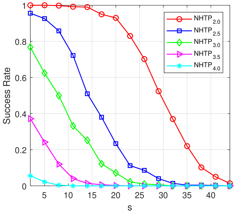
(a) Example 6.2

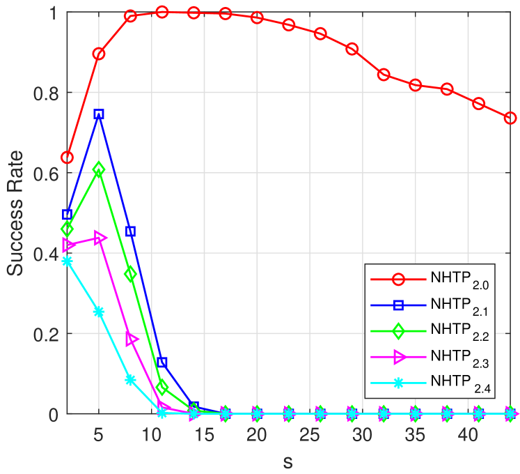
(b) Example 6.3

Figure 1: Success rates of NHTP_r. $n=200,s\in\{2,5,\cdots,44\}$.

Table 1: Comparison of NHTP_r with different $r$.

		$\|x-x^{*}\|/\|x^{*}\|$						Time (seconds)
Example 6.1
$n$		5000	10000	15000	20000	25000		5000	10000	15000	20000	25000
NHTP2.0		0.00e-0	0.00e-0	0.00e-0	0.00e-0	0.00e-0		0.004	0.005	0.007	0.009	0.014
NHTP2.5		5.65e-6	5.65e-6	5.65e-6	5.65e-6	5.65e-6		0.011	0.031	0.021	0.027	0.038
NHTP3.0		2.44e-4	2.44e-4	2.44e-4	2.44e-4	2.44e-4		0.011	0.021	0.025	0.029	0.038
NHTP3.5		7.84e-4	7.84e-4	7.84e-4	7.84e-4	7.84e-4		0.014	0.022	0.028	0.039	0.045
NHTP4.0		2.28e-3	2.28e-3	2.28e-3	2.28e-3	2.28e-3		0.018	0.062	0.031	0.040	0.047
Example 6.2
NHTP2.0		5.8e-12	6.4e-10	1.1e-12	1.4e-11	1.1e-10		0.064	0.188	0.394	0.699	1.021
NHTP2.5		3.61e-5	1.63e-6	9.88e-7	4.03e-6	3.07e-5		0.113	0.381	0.788	1.567	2.431
NHTP3.0		1.17e-2	9.03e-3	1.15e-2	4.12e-3	5.49e-3		0.173	0.540	1.169	2.423	4.075
NHTP3.5		3.10e-2	1.37e-2	1.57e-2	1.13e-2	7.82e-3		0.203	0.684	1.958	3.649	6.031
NHTP4.0		4.47e-2	2.25e-2	2.43e-2	4.92e-2	3.18e-2		0.227	0.800	2.563	5.150	7.179

To see the accuracy of the solutions and the speed of NHTP_r, we now test on two examples with higher dimensions $n$. For Example 6.1, we increase $n$ from $5000$ to $25000$ and fix $s^{*}=1$. Results are presented in Table 1. Whilst for Example 6.2, we run independent 20 trials for each $(n,s^{*})$ with $n$ ranging from $2000$ to $10000$ and fixing $s^{*}=0.01n$. Average results over 20 trials are presented in Table 1. Clearly, for both examples, NHTP₂ gets the most accurate solutions and runs the fastest for all cases. In a nutshell, the smaller $r$ is, the better NHTP performs.

6.3 Effect of $s$ with fixing $r=2$

To make results comparable, we fix $r=2$. In $S$, there is a parameter $s$ that should be given in advance. However, it is difficult to set an exact value for $s$ in practice. To see how the choices of $s$ affect the solution to (2), we apply NHTP  to address three examples with different

$${{s\in\{s^{*},\lceil 1.25s^{*}\rceil,\lceil 1.5s^{*}\rceil,\lceil 1.75s^{*}\rceil,2s^{*}\},}}$$

where $\lceil a\rceil$ returns the smallest integer that is no less than $a$. To see the recovery ability, we first apply them to solve Example 6.2 and Example 6.3 with fixing $n=200$ but with increasing sparsity level $s^{*}$ from $12$ to $80$. For each $(n,s^{*})$, we run $500$ independent trials and record the corresponding success rates in Figure 2, where data show that NHTP₂ with $s>s^{*}$ generates better success rates than $s=s^{*}$. More detailed, the larger $s$ is, the higher success rates are produced by NHTP₂. In addition, it seems to be more difficult for NHTP_r to solve Example 6.2 than Example 6.3. For instance, when $s=40$, NHTP₂ is able to recover $80\%$ trials for Example 6.3 while only get $5\%$ trials for Example 6.2.

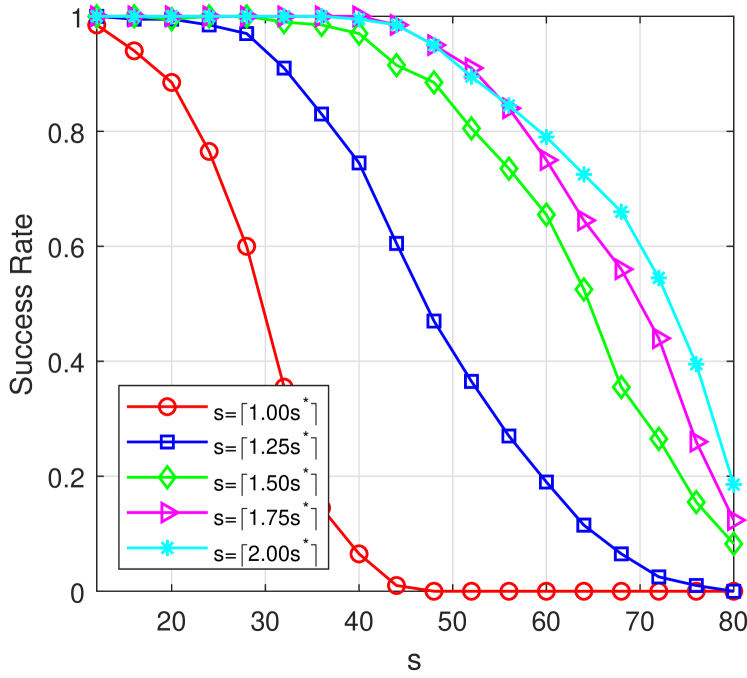
(a) Example 6.2

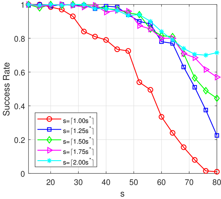
(b) Example 6.3

Figure 2: Success rates of NHTP₂. $n=200,s\in\{12,16,\cdots,80\}$.

Table 2: Comparison of NHTP₂ with different $s$.

	$\|x-x^{*}\|/\|x^{*}\|$						Time (seconds)
Example 6.1
$s\setminus n$	5000	10000	15000	20000	25000		5000	10000	15000	20000	25000
$\lceil 1.00s^{*}\rceil$	0.0e-0	0.0e-0	0.0e-0	0.0e-0	0.0e-0		0.007	0.009	0.010	0.012	0.012
$\lceil 1.25s^{*}\rceil$	0.0e-0	1.1e-16	0.0e-0	3.4e-21	0.0e-0		0.009	0.013	0.013	0.016	0.016
$\lceil 1.50s^{*}\rceil$	0.0e-0	1.1e-16	0.0e-0	3.4e-21	0.0e-0		0.008	0.014	0.013	0.016	0.016
$\lceil 1.75s^{*}\rceil$	0.0e-0	1.1e-16	0.0e-0	3.4e-21	0.0e-0		0.009	0.013	0.014	0.015	0.016
$\lceil 2.00s^{*}\rceil$	0.0e-0	1.1e-16	0.0e-0	3.4e-21	0.0e-0		0.008	0.015	0.014	0.016	0.017
Example 6.2
$\lceil 1.00s^{*}\rceil$	6.6e-13	4.8e-11	5.5e-12	7.3e-13	9.2e-11		0.05	0.19	0.38	0.68	1.10
$\lceil 1.25s^{*}\rceil$	5.4e-13	1.6e-10	1.1e-16	1.0e-13	3.9e-15		0.06	0.19	0.41	0.70	1.10
$\lceil 1.50s^{*}\rceil$	1.5e-14	9.2e-11	1.8e-14	5.4e-14	8.7e-16		0.06	0.19	0.42	0.71	1.13
$\lceil 1.75s^{*}\rceil$	4.6e-11	1.2e-10	2.3e-16	6.5e-14	9.3e-16		0.06	0.21	0.43	0.74	1.16
$\lceil 2.00s^{*}\rceil$	4.7e-11	1.2e-10	3.4e-14	2.2e-14	2.1e-15		0.06	0.21	0.45	0.77	1.21

We now increase $n$ from $5000$ to $25000$ and fix $s^{*}=1$ for Example 6.1. Related results are presented in Table 2. While for Example 6.2, we again run independent 20 trials for each $(n,s^{*})$ with $n$ ranging from $2000$ to $10000$ and keeping $s^{*}=0.01n$. Average results over 20 trials are presented in Table 2. For both tables, it can be clearly seen that accuracies obtained by NHTP₂ under different $s$ are similar. As expected, smaller $s$ enables NHTP₂ to run slightly faster than larger $s$.

6.4 Strategies to select $s$

Assume the sparse LCP (2) admits a sparsest solution $x^{*}$ with sparsity level $s^{*}$. As long as $s^{*}\ll n$ (e.g. $s^{*}\leq\lceil 0.1n\rceil$), numerical experiments in Section 6.3 demonstrate that NHTP achieves the sparsest solutions with a very high possibility if we set $s\geq s^{*}$, see Figure 2 for instance. Therefore, a possible way to tune a proper $s$ is designed as Algorithm 2, where parameter can be set as $s_{0}=\lceil n/5000\rceil$, $\varrho=\max\{2,\log_{10}(n)\}$ and $\epsilon=10^{-8}$. In this way, if (2) admits a solution $x^{*}$ with $s^{*}\ll n$, then the worst case to achieve $s\geq s^{*}$ is running NHTP $\lceil\log_{\varrho}(s^{*}/s_{0})\rceil$ times, after which NHTP will possibly achieve the solution.

Algorithm 2 NHTPT: NHTP with sparsity level tuning

  Initialize a small integer $s_{0}\in{\mathbb{N}},\varrho>1,\epsilon>0$ and $x^{0}=0$. Set $\ell\Leftarrow 0$.

  while $f_{r}(x^{\ell})\geq\epsilon$ do

      Set $s=s_{\ell}$ and run NHTP in Algorithm 1 to generate a solution $x^{\ell+1}$

      Set $s_{\ell}=\lceil\varrho s_{\ell}\rceil$ and $\ell\Leftarrow\ell+1.$

  end while

  return  the solution $x^{\ell}$.

An alternative takes advantage of other methods that do not need the prior information $s$, for example, Lemke’s (Lemke ) algorithm, a well-known high standard method to solve the LCP. Therefore, we could first run Lemke to obtain a solution $x_{\rm lem}$ and then set $s=\|x_{\rm lem}\|_{0}$ for NHTP. Note that $\|x_{\rm lem}\|_{0}$ actually provides an upper bound of $s$. However, we test that this upper bound sometimes is good enough.

Now we would like to see the performance of Lemke, NHTP with the help of $s=\|x_{\rm lem}\|_{0}$ and NHTPT in Algorithm 2. We fix $r=2$ in $f_{r}$ for the latter two methods. Average results over 20 trials are presented in Table 3, where all methods achieve solutions to LCP for all cases since the objective values $f_{r}$ are close to zeros. For Example 6.2, where the ‘ground truth’ solutions are given and $s^{*}$ is set as $\lceil 0.01n\rceil$, three methods render solutions with sparsity levels being identical to $s^{*}$. NHTP runs the fastest, followed by NHTPT. While Lemke consumes too much time, e.g., 78.27 seconds v.s. 7.3 seconds by NHTP when $n=25000$. For Example 6.4, the ‘ground truth’ solutions are unknown and $s^{*}$ is set as $\lceil 0.5n\rceil$. Note that this large $s^{*}$ for such example is not the sparsity level of a solution, but can be an upper bound of $s$. As shown in Table 3, three methods succeed in finding very sparse solutions since the sparsity levels $\|x\|_{0}$ are relatively small to the large $s^{*}$. In addition, NHTPT runs the fastest and also produces the sparsest solutions, followed by NHTP.

The performance of NHTPT solving the above two examples illustrates that the strategy in Algorithm 2 allows NHTP to find a proper $s$ iteratively. However, in the sequel, we still focus on NHTP itself instead of NHTPT for the sake of simplicity.

Table 3: Comparison of Lemke, NHTP and NHTPT.

	$f_{2}$				Time (seconds)				$\|x\|_{0}$
$n$	Lemke	NHTP	NHTPT		Lemke	NHTP	NHTPT		Lemke	NHTP	NHTPT
	Example 6.2
5000	6.63e-30	5.22e-15	3.78e-14		0.63	0.27	0.61		50	50	50
10000	1.32e-29	2.25e-14	9.35e-15		3.81	0.95	2.05		100	100	100
15000	3.09e-29	7.36e-15	3.68e-15		12.1	2.03	4.41		150	150	150
20000	4.93e-29	6.77e-15	5.39e-15		27.6	3.55	7.90		200	200	200
25000	1.09e-28	4.82e-14	3.23e-16		78.3	7.30	12.7		250	250	250
	Example 6.4
5000	3.63e-09	1.50e-12	2.45e-11		0.43	0.28	0.16		25.7	25.7	1.0
10000	1.23e-08	8.35e-11	7.25e-12		1.29	0.62	0.48		21.4	21.4	2.0
15000	4.44e-09	5.44e-12	2.64e-12		2.90	1.16	1.10		10.8	10.8	2.9
20000	9.87e-09	1.12e-12	2.04e-12		5.21	1.88	1.79		6.3	6.3	4.0
25000	1.65e-08	2.14e-12	1.20e-12		30.2	4.90	2.76		5.9	5.9	4.9

6.5 Numerical comparisons

Since there are very few methods that have been proposed to process the sparse LCP, we compare NHTP_r only with half thresholding projection (HTP) method [35] and extra-gradient thresholding algorithm (ETA) [33]. We use all their default parameters and terminate both of them when $\|x^{k}-z^{k}\|<10^{-5}\max\{1,\|x^{k}\|\}$ or the maximum number of iterations reach 2000. Note that both methods make use of the first order information of the involved functions and thus belong to the class of the first order methods. NHTP uses the origin as its default starting point. However, as a second order method, it is suggested to start from a local area around a solution. Therefore, we take advantage of the solution obtained by HTP as the starting point of NHTP. Under such circumstance, write NHTP_r as HNHTP_r. We thus compare NHTP₂, HNHTP₂, HNHTP_2.5, HNHTP₃, HTP and ETA. For the former four NHTP-related methods, we choose $s=s^{*}$ in $S$ for Example 6.1, Example 6.2 and Example 6.3 since the sparsity of the ‘ground truth’ solution is $s^{*}$ and choose

$$s=\min\{\|x_{\texttt{HTP}}\|_{0},\|x_{\texttt{ETA}}\|_{0},s^{*}\}.$$

for Example 6.4 since the ‘ground truth’ solution is unknown, where $x_{\texttt{HTP}}$ and $x_{\texttt{ETA}}$ are solutions produced by HTP and ETA, respectively. In such a way, NHTP could always get solutions that are sparser than solutions produced by the last two methods.

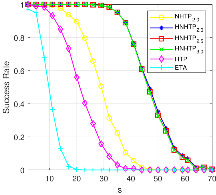
(a) Example 6.2

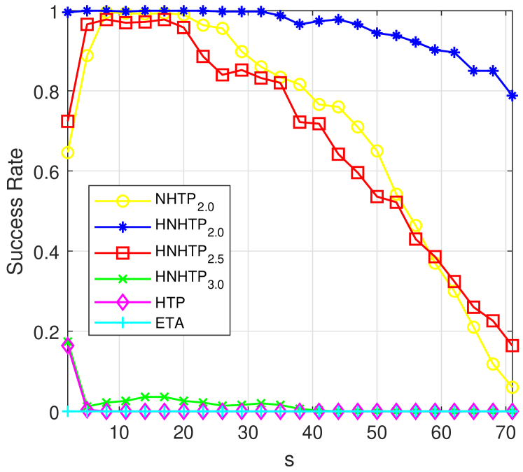
(b) Example 6.3

Figure 3: Success rates of NHTP, HTP and ETA. $n=200,s\in\{2,5,\cdots,71\}$.

(a) Recovery ability. Similarly, to see the recovery ability, we first apply them to solve Example 6.2 and Example 6.3 with fixing $n=200$ but with increasing sparsity level $s^{*}$ from $2$ to $71$. For each $(n,s^{*})$, we run $500$ independent trials and record the corresponding success rates in Figure 3, where data in subfigure (a) show that HNHTP₂, HNHTP_2.5, HNHTP₃ generate similar results and obtain the highest success rates, followed by NHTP₂. While HTP and ETA come the last. When those methods are applied to solve Example 6.3, the results in subfigure (b) present a big different picture. HNHTP₂ outperforms the other five methods, followed by NHTP₂, HNHTP_2.5. In contrast, HNHTP₃ HTP and ETA basically fail to recover solutions for cases of $s\geq 5.$ Overall, one could conclude that HTP itself does not produce accurate solutions but could offer good starting points, from which HNHTP₂, HNHTP_2.5, HNHTP₃ benefit significantly.

(b) Accuracy and speed in the higher dimensional setting. To see the performance of six methods on solving larger size problems, we now increase $n$ from $5000$ to $25000$ and fix $s^{*}=1$ for Example 6.1. Related results are presented in Table 4. For Example 6.2, we again run independent 20 trials for each $(n,s^{*})$ with $n$ ranging from $2000$ to $10000$ and keeping $s^{*}=0.01n$. Average results over 20 trials are presented in Table 4. It can be clearly seen that HNHTP₂ and NHTP₂ get the most accurate solutions, followed by HNHTP_2.5 and HNHTP₃, HTP comes the last. For the computational time, all NHTP methods run much faster than HTP and ETA.

Table 4: Comparison of NHTP_r, HTP and ETA.

		$\|x-x^{*}\|/\|x^{*}\|$						Time (seconds)
Example 6.1
$n$		5000	10000	15000	20000	25000		5000	10000	15000	20000	25000
NHTP2.0		0.00e-0	0.00e-0	0.00e-0	0.00e-0	0.00e-0		0.004	0.006	0.008	0.007	0.009
HNHTP2.0		0.00e-0	0.00e-0	0.00e-0	0.00e-0	0.00e-0		0.003	0.005	0.007	0.006	0.009
HNHTP2.5		3.89e-6	3.89e-6	3.89e-6	3.89e-6	3.89e-6		0.006	0.010	0.014	0.020	0.017
HNHTP3.0		7.88e-5	7.87e-5	7.87e-5	7.87e-5	7.87e-5		0.004	0.006	0.007	0.012	0.010
HTP		3.15e-4	3.15e-4	3.15e-4	3.15e-4	3.15e-4		0.037	0.086	0.132	0.163	0.171
ETA		2.93e-4	2.93e-4	2.93e-4	2.93e-4	2.93e-4		0.077	0.193	0.282	0.498	0.378
Example 6.2
NHTP2.0		2.0e-12	2.5e-11	1.3e-12	1.0e-13	1.5e-13		0.08	0.21	0.40	0.73	1.02
HNHTP2.0		6.7e-12	1.3e-10	1.7e-11	1.0e-11	4.2e-11		0.05	0.18	0.35	0.62	0.98
HNHTP2.5		1.76e-7	8.51e-8	7.98e-8	7.95e-8	1.41e-7		0.10	0.33	0.66	1.18	1.90
HNHTP3.0		4.41e-6	1.61e-6	1.51e-6	2.71e-6	4.48e-6		0.09	0.30	0.60	1.04	1.70
HTP		2.38e-4	3.17e-4	2.94e-4	2.85e-4	4.21e-4		1.61	6.96	13.7	24.6	41.8
ETA		2.01e-4	1.76e-4	1.73e-4	1.69e-4	2.71e-4		3.07	15.1	30.9	56.6	88.4

Table 5: Comparison of NHTP_r, HTP and ETA.

		$f_{2}(x)$						Time (seconds)
$n$		2000	4000	6000	8000	10000		2000	4000	6000	8000	10000
NHTP2.0		9.65e-8	1.25e-7	3.08e-8	1.22e-7	1.10e-7		0.04	0.04	0.07	0.12	0.16
HNHTP2.0		7.63e-6	1.79e-8	1.41e-8	1.29e-7	4.52e-8		0.07	0.04	0.05	0.07	0.11
HNHTP2.5		6.08e-5	2.66e-5	1.13e-8	1.69e-8	1.63e-8		0.02	0.04	0.06	0.09	0.12
HNHTP3.0		8.72e-5	3.33e-4	5.34e-4	7.07e-4	7.65e-4		0.01	0.02	0.02	0.04	0.05
HTP		9.66e-5	1.89e-4	2.86e-4	3.68e-4	4.50e-4		0.03	0.03	0.04	0.04	0.05
ETA		1.84e-4	1.94e-4	2.39e-4	2.50e-4	3.09e-4		0.27	1.51	3.65	7.24	12.2
		$\|\nabla f_{2}(x)\|$						$\|x\|_{0}$
NHTP2.0		1.14e-4	2.05e-5	1.37e-5	3.30e-5	2.60e-5		9.2	15.0	19.3	24.3	30.5
HNHTP2.0		1.93e-4	1.70e-5	2.39e-5	7.26e-5	3.67e-5		9.0	14.8	19.3	24.3	30.5
HNHTP2.5		1.86e-3	3.02e-3	3.90e-3	5.86e-3	7.58e-3		9.2	15.0	19.3	24.3	30.5
HNHTP3.0		4.85e-2	1.20e-2	7.24e-2	1.92e-1	2.74e-1		9.2	15.0	19.3	24.3	30.5
HTP		2.12e-3	4.77e-3	7.45e-3	1.04e-2	1.30e-2		11.3	27.1	44.8	64.8	81.7
ETA		3.30e-3	4.87e-3	6.68e-3	8.11e-3	1.02e-2		9.2	15.0	19.3	24.3	30.5

(c) Performance on solving examples without known solutions. Now we compare those methods on solving Example 6.4, where solutions are unknown. Nevertheless, they possibly admit some sparse solutions by Theorem 4.3. We run independent 20 trials for each $(n,s^{*})$ with $n$ ranging from $2000$ to $10000$ and keeping $s^{*}=0.01n$. Average results are presented in Table 5. Note that since the objective functions $f_{r}$ is different with different $r$, to make comparison reasonable, we calculate $f_{2}(x)$, where $x$ is generated by one of six methods. For Example 6.4, all NHTP-related methods get the smallest objective function values and $\|\nabla f_{2}(x)\|$ with the sparsest solutions, which means they outperform HTP and ETA in terms of the quality of solutions. In addition, HTP always obtains solutions that are least sparse, but it and HNHTP_3.0 run the fastest. ETA is the slowest one again.

6.6 Comparison of different NCP functions

For the sake of illustrating the advantage of $\phi_{r}$, we make use of NHTP to address the problem (6) with different objective functions constructed by three NCP functions $\phi_{FB}$, $\phi_{\min}$ and $\phi^{2}_{II}$ from Remark 2.3. The corresponding merit functions are

$$f_{FB}(x) = 0.5\sum(\phi_{FB}(x_{i},y_{i}))^{2}$$

$$= 0.5\left[\|x\|^{2}+\|y\|^{2}+\|x+y\|^{2}-2\langle\sqrt{x\circ x+y\circ y},x+y\rangle\right],$$

$$f_{\min}(x) = 0.5\sum(\phi_{\min}(x_{i},y_{i}))^{2}$$

$$= 0.5[\|x+y\|^{2}+\|x-y\|^{2}-2\langle\sqrt{(x-y)\circ(x-y)},x+y\rangle],$$

$$f_{II}(x) = 0.5\sum(\phi^{2}_{II}(x_{i},y_{i}))^{2}=0.5\left[\|(x\circ y)_{+}\|^{2}+\|x_{-}\|^{2}+\|y_{-}\|^{2}\right],$$

where $\sqrt{z}=(\sqrt{z_{1}},\cdots,\sqrt{z_{n}})^{\top}$ and $y=Mx+q$.

Remark 6.5.

We have some comments about the above merit functions and $f_{2}$.

• Note that $f_{FB}$ and $f_{\min}$ have unbounded Hessian at $(0,0)$ and $x=y$, respectively. Therefore, to make use of NHTP, we add a small scalar $\varepsilon$ (e.g. $10^{-10}$) to smooth $\sqrt{z}$, namely, replacing $\sqrt{z}$ by $\sqrt{z+\varepsilon}$ in $f_{FB}$ and $f_{\min}$. Then their gradients and Hessian are able to be derived. In addition, similar rules to calculate $\partial^{2}f_{2}(x)$ in (3)) also lead to the generalized Hessian of $f_{II}$.

• As shown in [41], to derive the Newton direction, each step in NHTP  calculates a submatrix $\nabla_{TT}^{2}f(x)$ of the Hessian of $f$. It is easy to see that the Hessians of $f_{FB}$ and $f_{\min}$ have a term $M^{\top}M$. Therefore, we need to compute $M_{T}^{\top}M_{T}$ and the computational complexity is about $\mathcal{O}(ns^{2})$. While for $f_{II}$ and $f_{2}$, the most expensive computation is $M_{T}^{\top}{\rm Diag}(\zeta)M_{T}$. When the point is close to a solution to the LCP, then $y\geq 0$, which together with (29) indicates

  $$M_{T}^{\top}{\rm Diag}(\zeta)M_{T}=M_{{\rm supp}(x)T}^{\top}{\rm Diag}(\zeta_{{\rm supp}(x)})M_{{\rm supp}(x)T}.$$

  This means the computational complexity is about $\mathcal{O}(s^{3})$. Therefore, we expect that $f_{FB}$ and $f_{\min}$ take longer time to do computations than $f_{II}$ and $f_{2}$ in each step, which is testified by the numerical experiments in the sequel.

Now we apply NHTP with fixing $s=s^{*}=0.01n$ to process the sparsity constrained model (6) with four merit functions $f_{FB}$, $f_{\min}$, $f_{II}$ and $f_{2}$. To see the decline of objective function values in each step at the beginning of the method, we report $f_{2}(x)$ to make results comparable, where $x$ is generated by NHTP solving sparsity constrained model with one of there merit functions. For example, we record the iterates $x^{1},x^{2},\cdots$ generated by NHTP under $f_{FB}$ and then calculate $f_{2}(x^{1}),f_{2}(x^{2}),\cdots$. Results are presented in Figure 4. It is worth mentioning that all merit functions make NHTP get the global solutions eventually, while we only report results at first 22 or 50 iterations. The prominent feature of the four sub-figures is that the lines of $f_{2}$ drop dramatically for all examples. It only takes less than five steps to reduce the objective almost to zero. By contrast, when NHTP addresses the model with $f_{II}$, much more steps are required and the objective function values decline relatively slowly. This phenomenon also appears for Example 6.4, where NHTP seems not to prefer the sparsity constrained models with $f_{FB}$, $f_{\min}$ and $f_{II}$.

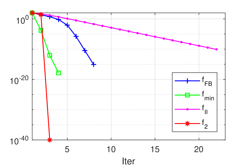
(a) Example 6.1

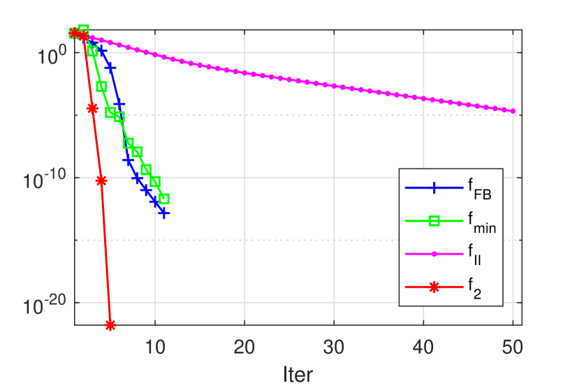
(b) Example 6.2

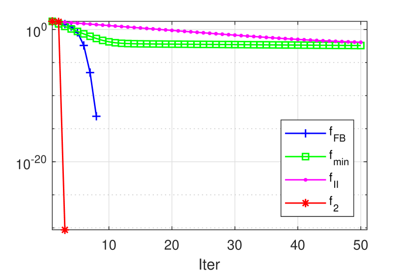
(c) Example 6.3

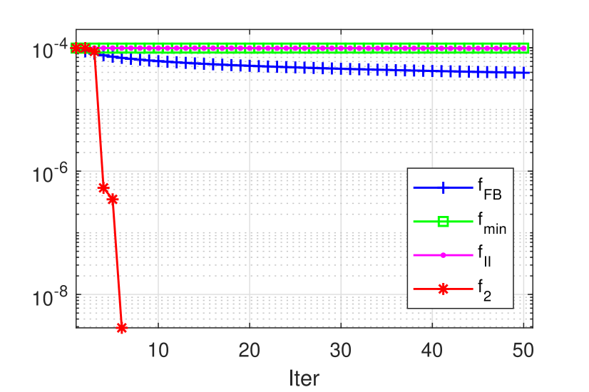
(d) Example 6.4

Figure 4: Objective function values $f_{2}$ at first 20 or 50 iterations. $n=200,s=2$.

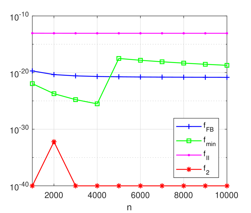
(a) Example 6.1: $f_{2}(x)$

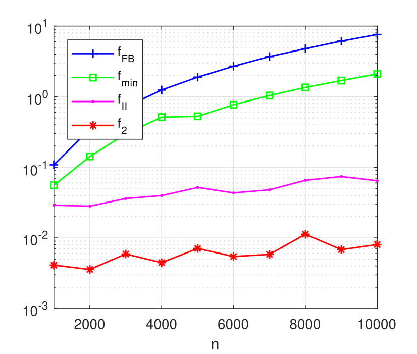
(b) Example 6.1: Time

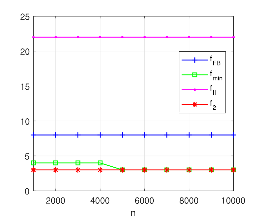
(c) Example 6.1: Iteration

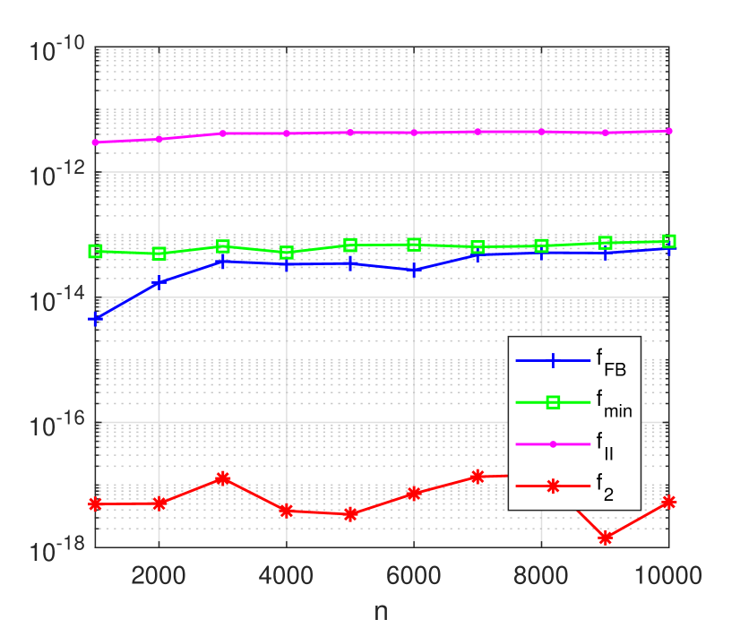
(d) Example 6.2: $f_{2}(x)$

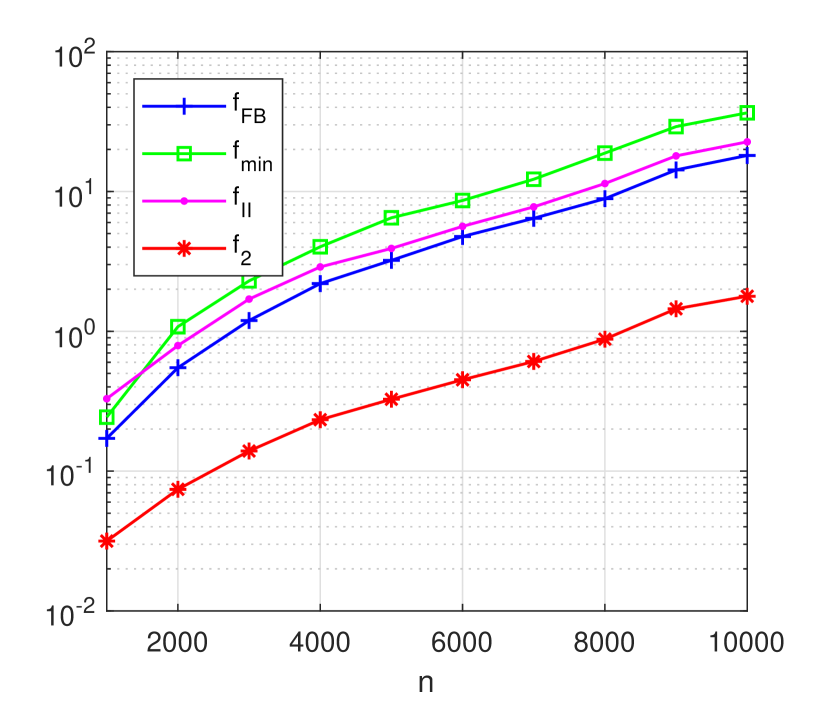
(e) Example 6.2: Time

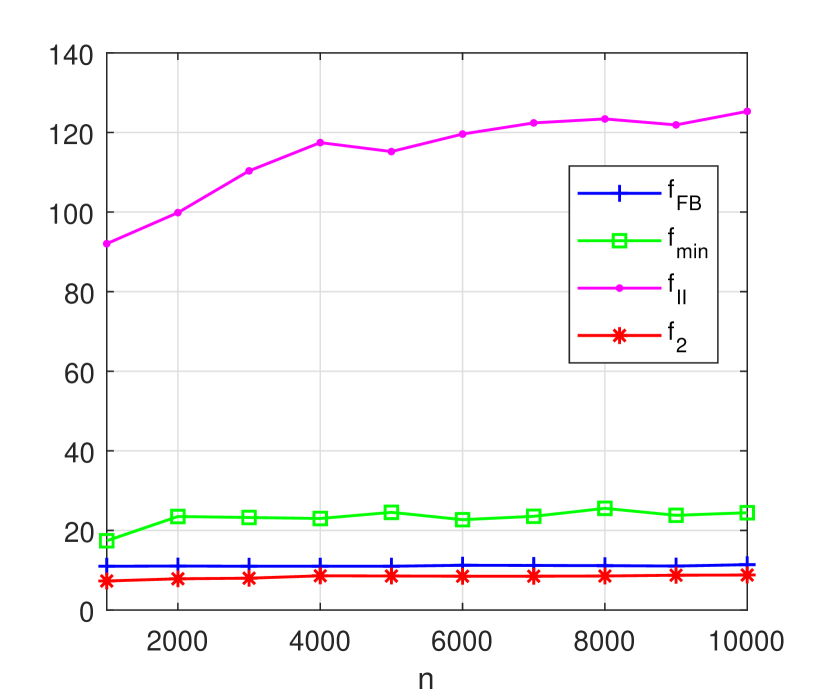
(f) Example 6.2: Iteration

Figure 5: Comparison of NHTP solving the sparsity constrained model with four functions.

We now solve the sparsity constrained model with higher dimensions $n$, and only present results of Example 6.1 and Example 6.2 in Figure 5, since the results of the rest examples are similar. In terms of accuracy, $f_{2}$ outperforms the others since it obtains smallest objective function values, with the order of $10^{-17}$ from $f_{2}$ v.s. $10^{-12}$ from $f_{II}$ in sub-figure (d). For the computational speed, it can be clearly seen that $f_{2}$ allows NHTP to run the fastest. By contrast, $f_{FB}$ and $f_{\min}$ run the slowest for Example 6.1 and Example 6.2, respectively. More detailed, as expected, $f_{FB}$ and $f_{2}$ for Example 6.2 in (f) (or $f_{\min}$ and $f_{2}$ for Example 6.1 in (c)) need similar number of iterations. However, the model with $f_{2}$ makes the method take much shorter CPU time, which means the computational complexity in each step is much lower. Finally, again $f_{II}$ leads to NHTP  using more iterations and thus consuming longer total time than that from $f_{2}$. In summary, among these merit functions, the sparsity constrained model with $f_{2}$ allows NHTP to run the fastest to get the most desirable solutions.

7 Conclusion

A new merit function $f_{r}$ has been introduced to convert the sparse LCP into a sparsity constrained optimization, enjoying many properties, such as being continuously differentiable for any $r\geq 2$, twice continuously differentiable for any $r>2$, and convex if the matrix is positive semidefinite. The relationship between the stationary points to the sparsity constrained optimization and solutions to the sparse LCP has been well revealed. Numerical experiments demonstrated that the adopted method NHTP has excellent performance to solve the sparsity constrained optimization. Most importantly, comparing the merit functions constructed from other existing famous NCP functions, the optimization with our merit function $f_{r}$ enables NHTP to possess the lowest computational complexity, fastest convergent speed and most desirable accuracy. As a result, through converting the sparse LCP into the sparsity constrained optimization with the help of $f_{r}$, it can be effectively solved by NHTP. In addition, we feel that the new proposed NCP function $\phi_{r}$ might be able to deal with the sparse nonlinear complementarity problem. We will explore more on this topic in future.

Appendix A Proof of theorems in Section 2 - Section 5

A.1 Proof of Proposition 2.5

The result 1) is taken from [5, Theorem 3.3.4]. We prove the second claim. If $A$ is a P_s-matrix, then for each nonzero $x\in{\mathbb{R}}^{n}$ with $T:={\rm supp}(x)$ and $|T|=\|x\|_{0}\leq s$, $A_{TT}$ is a $P$ matrix by the definition of P_s-matrix. This implies there is an $i\in T$ such that $x_{i}(Ax)_{i}=x_{i}(A_{TT}x_{T})_{i}>0.$ Conversely, if for each nonzero $x\in{\mathbb{R}}^{n}$ with $T={\rm supp}(x)$ and $|T|\leq s$, then there is an $i$ such that $x_{i}(Ax)_{i}>0.$ Clearly, such $i\in T$. Since $(Ax)_{T}=A_{TT}x_{T}$, this statement is equivalent to that for each given $T$ with $|T|\leq s$, for each nonzero $z\in{\mathbb{R}}^{|T|}$, there is a $j$ such that $z_{j}(A_{TT}z)_{j}>0$. Therefore, $A_{TT}$ is a P-matrix. Moreover, $T$ can be any subset of ${\mathbb{N}}$ with $|T|\leq s$, so any $A_{TT}$ is a P-matrix, which means $A$ is a $P_{s}$ matrix.

A.2 Proof of Lemma 3.1

1) It follows from Proposition 2.1 that $\phi_{r}(a,b)$ is continuously differentiable. This together with $x_{i}=\langle e_{i},x\rangle$ and $y_{i}=M_{i}x+q_{i}$ both being continuously differentiable leads to $\phi_{r}(x_{i},y_{i})$ being also continuously differentiable. Then the $\nabla f_{r}(x)$ is derived by the addition and chain rules, namely,

$$\nabla f_{r}(x) = \sum\left[\partial_{1}\phi_{r}(x_{i},y_{i})\nabla x_{i}+\partial_{2}\phi_{r}(x_{i},y_{i})\nabla y_{i}\right]$$

$$= \sum\left[\left((x_{i})_{+}^{r-1}(y_{i})_{+}^{r}-|(x_{i})_{-}|^{r-1}\right)e_{i}+\left((x_{i})_{+}^{r}(y_{i})_{+}^{r-1}-|(y_{i})_{-}|^{r-1}\right)M_{i}^{\top}\right]$$

$$= x_{+}^{r-1}\circ y_{+}^{r}-|x_{-}|^{r-1}+M^{\top}\left[x_{+}^{r}\circ y_{+}^{r-1}-|y_{-}|^{r-1}\right].$$

2) For $r>2$, $\nabla f_{r}(x)$ is continuously differentiable because all involved functions in $\nabla f_{r}(x)$ are continuously differentiable. We omitted the detailed calculations here since the addition and chain rules enable us to derive $\nabla^{2}f_{r}(x)$ directly.

3) When $r=2$, it follows

$$\nabla f_{2}(x)=x_{+}\circ y_{+}^{2}-|x_{-}|+M^{\top}\left[x_{+}^{2}\circ y_{+}-|y_{-}|\right]=\underset{=:g(x)}{\underbrace{x_{+}\circ y_{+}^{2}+x_{-}}}+\underset{=:h(x)}{\underbrace{M^{\top}\left[x_{+}^{2}\circ y_{+}+y_{-}\right]}}.$$

Then from [4, Proposition 1.12] or [16, Example 2.6], we have

$$\partial^{2}f_{2}(x)=\partial(\nabla f_{2}(x))\subseteq\partial g(x)+\partial h(x).$$

Therefore, the next step is to calculate $\partial g(x)$ and $\partial h(x)$. For each $g_{i}(x)$, we have

$$g_{i}(x)=\left(x_{+}\circ y_{+}^{2}+x_{-}\right)_{i}=\left\{\begin{array}[]{ccc}x_{i}(y_{i})_{+}^{2},&x_{i}>0,\\ x_{i},&x_{i}\leq 0.\end{array}\right.$$

It is easy to obtain that the generalized Jacobian of $g_{i}(x)$ by

$$\partial g_{i}(x)=\left\{\begin{array}[]{rr}\left\{2x_{i}(y_{i})_{+}M^{\top}_{i}+(y_{i})_{+}^{2}e_{i}\right\},&x_{i}>0,\\ {\rm co}\left\{e_{i},(y_{i})_{+}^{2}e_{i}\right\},&x_{i}=0,\\ \left\{e_{i}\right\},&x_{i}<0,\end{array}\right.$$

which implies that

$$\partial g(x)=\{~{}2{\rm Diag}(x_{+}\circ y_{+})M+{\rm Diag}(\xi):~{}\xi\in\Omega_{\xi}(x)~{}\},$$

where $\Omega_{\xi}(x)$ is given by (28). Similar reasoning also allows us to derive

$$\partial h(x)=\{~{}2M^{\top}{\rm Diag}(x_{+}\circ y_{+})+M^{\top}{\rm Diag}(\zeta)M:~{}\zeta\in\Omega_{\zeta}(x)~{}\},$$

where $\Omega_{\zeta}(x)$ is given by (29). Those prove the claim.

4) For any $r\geq 2$, it follows from (2)) and (3)) that $\nabla^{2}f_{r}(x)$ and any element in $\partial^{2}f_{2}(x)$ are positive semidefinite if $M\succeq 0$ and thus $f_{r}(x)$ is convex.

A.3 Proof of Theorem 3.2

1) If $M$ is positive semidefinite and fea(M,q) is nonempty, it follows from [5, Theorem 3.1.2] that sol(M,q) is nonempty. Then ${\texttt{sol}(M,q)}={\rm argmin}_{x}\ f_{r}(x)$ by (32). Again $M$ being positive semidefinite results in the convexity of $f_{r}$ from Lemma 3.1 4), which means a point $x^{*}$ is a solution to ${\min}_{x}\ f_{r}(x)$ if and only if $\nabla f_{r}(x^{*})=0$, namely, a stationary point.

2) If $M$ is a P-matrix, we can conclude from [19, Theorem 5.1, Lemma 5.2] that a point is a solution to (1) if and only if it is a stationary point. Thus we have sol(M,q)$=\mathcal{G}_{f}$. Then by [5, Theorem 3.3.7] or [32, Theorem 1.4], (1) has a unique solution for all $q\in{\mathbb{R}}^{n}$ if and only if $M$ is a P-matrix.

A.4 Proof of Lemma 4.1

The problem (34) is equivalent to

(63) $$\underset{T\subseteq{\mathbb{N}},|T|\leq s}{{\rm min}}\left\{\underset{x}{\rm min}~{}\langle x,Mx+q\rangle,~{}~{}{\rm s.t.}~{}x_{T}\geq 0,x_{T^{c}}=0,Mx+q\geq 0\right\}.$$

Since fea${}_{s}(M,q)$ is nonempty, there are some $T$ with $T\subseteq{\mathbb{N}},|T|\leq s$ such that the inner program of (63) is feasible. This together with the Frank-Wolfe theorem [11] implies that the inner program admits an optimal solution $x(T)$ because it is a quadratic program being bounded from below over the feasible region. Clearly, the optimal function value denoted as $\gamma_{T}$ is unique. As the choices of $T$ are finitely many, e.g., $T\in\{T_{1},\cdots,T_{N}\}$, there are finitely many $\gamma_{T}$. To derive the optimal solution of (34), we can pick one $T_{i}$ from $\{T_{1},\cdots,T_{N}\}$ such that the objective function value $\gamma_{T_{i}}$ is the smallest. Then $x(T_{i})$ is an optimal solution of (34), namely, $Q_{s}(M,q)$ is nonempty.

A.5 Proof of Theorem 4.2

1) Since $M$ is symmetric, $M_{T}$ having full column rank means that $\{M_{i}^{\top}:i\in T\}$ are linearly independent. Then it follows from this fact and [27, Corollary 2.8, Theorem 3.6], a global optimal solution $x$ with $\|x\|_{0}=s$ satisfies the following first order optimality conditions, for some $u\in{\mathbb{R}}^{n}$,

(67) $$\left\{\begin{array}[]{r}M_{TT}x_{T}+q_{T}+M_{TT}x_{T}-M_{T\Gamma}u_{\Gamma}=0,\\ x_{T}>0,~{}x_{T^{c}}=0,~{}u_{\Gamma}\geq 0,~{}u_{\Gamma^{c}}=0,\\ M_{\Gamma T}x_{T}+q_{\Gamma}=0,~{}M_{\Gamma^{c}T}x_{T}+q_{\Gamma^{c}}>0.\end{array}\right.$$

where $T$ and $\Gamma$ are defined in (35). We now prove that $T\subseteq\Gamma$. In fact, if there is an $j\in T$ but $j\notin\Gamma$, we have $M_{jT}x_{T}+q_{j}>0$ from the last inequality in (67), which derives that $M_{jT}x_{T}>-q_{j}\geq 0$ by assumption $q_{T}\leq 0.$ Now consider the first equation in (67),

$$0=M_{jT}x_{T}+q_{j}+M_{jT}x_{T}-M_{j\Gamma}u_{\Gamma}>-M_{j\Gamma}u_{\Gamma}\geq 0$$

due to $M$ being a Z-matrix, $j\notin\Gamma$ and $u_{\Gamma}\geq 0$. Clearly, this is a contradiction. Therefore, we have $T\subseteq\Gamma$, namely, $M_{TT}x_{T}+q_{T}=0$, which gives rise to $\langle x,Mx+q\rangle=\langle x_{T},M_{TT}x_{T}+q_{T}\rangle=0$. Thus $x\in{\texttt{sol}(M,q)}$, showing $x\in{\texttt{sol}(M,q)}\cap S$.

2) Since $M$ is symmetric, $M_{T\Gamma}$ having full column rank means that $\{M_{iT}^{\top}:i\in T\}$ are linearly independent. From this and [27, Corollary 2.8, Theorem 3.6], a global optimal solution $x$ with $\|x\|_{0}<s$ satisfies the following first order optimality conditions, for some $u,v\in{\mathbb{R}}^{n}$,

(71) $$\left\{\begin{array}[]{r}Mx+q+Mx-v-Mu=0,\\ x\geq 0,~{}v\geq 0,~{}\langle x,v\rangle=0,\\ {{u\geq 0,~{}Mx+q\geq 0,~{}\langle u,Mx+q\rangle=0.}}\\ \end{array}\right.$$

In addition, $v_{T}=0$ by $x_{T}>0$ and $\langle x,v\rangle=0$. This and the above conditions suffice to (67). Then the rest of proof is the same as that of proving 1).

3) Since $M$ is symmetric, $M_{T\Gamma}$ having full column rank means that $\{M_{iT}^{\top}:i\in T\}$ are linearly independent. By 2), we obtain (71) which can be rewritten as the conditions that are identical to ones presented in [2, Lemma 3.1.1]. Then $M$ being positive semidefinite and [2, Theorem 3.1.2] allow us to conclude the result.

A.6 Proof of Theorem 4.3

If $|\theta|$=0, then $q\geq 0$, which results in $x^{*}=0$ being a solution to (2), and thus the conclusion holds immediately. Now consider $0<|\theta|\leq s$. Clearly, $M_{\theta\theta}$ is a P matrix since $M$ is a P_s matrix. This and Theorem 3.2 2) allow us to conclude that there is a unique solution $u$ satisfying

(72) $$u\geq 0,~{}~{}M_{\theta\theta}u+q_{\theta}\geq 0,~{}~{}\langle u,M_{\theta\theta}u+q_{\theta}\rangle=0.$$

Since $M\geq 0$ and $q_{\theta^{c}}\geq 0$ because of $0<|\theta|\leq s$, we have $M_{\theta^{c}\theta}u+q_{\theta^{c}}\geq 0$. Finally, by letting $x^{*}_{\theta}=u$ and $x^{*}_{\theta^{c}}=0$, we have $x^{*}\in({\texttt{sol}(M,q)}\cap S)$. To see the uniqueness, assume there is another point $z\in({\texttt{sol}(M,q)}\cap S)$ with ${\rm supp}(z)\subseteq\theta$. Clearly, $z_{\theta}$ satisfies (72). However, (72) only admits one solution $u$. Therefore, $z_{\theta}=u=x_{\theta}$.

A.7 Proof of Theorem 4.4

Suppose there is an unbounded subsequence of $\{x^{k}\}_{k\in K}\subseteq\mathcal{L}_{s}(f_{r},\gamma)$ for some $\gamma\geq 0$, where $K$ is a subset of $\{1,2,\cdots\}$. Let the index set $J:=\{i\in{\mathbb{N}}:~{}\{x_{i}^{k}\}~{}{\rm is~{}unbounded}\},$ which is nonempty due to $\{x^{k}\}_{k\in K}$ being unbounded. Now define a bounded sequence $\{z^{k}\}$ by

$$z_{i}^{k}=\left\{\begin{array}[]{cc}0,&i\in J,\\ x_{i}^{k},&i\notin J.\end{array}\right.$$

Clearly, we have $z^{k}\in S$ and $x^{k}-z^{k}\in S$ due to $x^{k}\in S$. Now since $M$ is a P_s matrix (see Proposition 2.5), then there exists a $\tau>0$ such that $\max_{j}(z_{j}M_{j}z)\geq\tau\|z\|^{2}$ for each nonzero $z\in S$. In fact, if for any $\tau>0$, there is a nonzero $z\in S$ such that $\max_{j}(z_{j}M_{j}z)<\tau\|z\|^{2}$, then we have $z^{\top}Mz=\sum_{j}z_{j}M_{j}z<n\tau\|z\|^{2}$, which leads to

$$\tau>\frac{z^{\top}Mz}{n\|z\|^{2}}=\frac{z_{T}^{\top}M_{TT}z_{T}}{n\|z_{T}\|^{2}}\geq\frac{\sigma_{\min}(M_{TT})}{n}>0,$$

where $\sigma_{\min}(M_{TT})$ is positive due to $M_{TT}$ being a P matrix from $M$ being a P_s matrix, which is a contradiction if $\tau$ is sufficiently small. So, the above assertion indicates

$$\tau\sum_{i\in J}(x_{i}^{k})^{2} = \tau\|x^{k}-z^{k}\|^{2}\leq\max_{j}~{}(x^{k}_{j}-z^{k}_{j})M_{j}(x^{k}-z^{k})$$

$$= \max_{j\in J}~{}(M_{j}x^{k}-M_{j}z^{k})(x^{k}_{j}-z^{k}_{j})=(M_{j_{0}}x^{k}-M_{j_{0}}z^{k})x^{k}_{j_{0}}$$

$$\leq (|M_{j_{0}}x^{k}|+|M_{j_{0}}z^{k}|)|x^{k}_{j_{0}}|,$$

where the first inequality comes from $x^{k}-z^{k}\in S$ and $j_{0}$ is one of the indices for which the max is attained. This inequality divided by $|x^{k}_{j_{0}}|$ on both sides derives that

$$\tau|x^{k}_{j_{0}}|\leq\tau|x^{k}_{j_{0}}|+\tau\sum_{i(\neq j_{0})\in J}(x_{i}^{k})^{2}/|x^{k}_{j_{0}}|\leq|M_{j_{0}}x^{k}|+|M_{j_{0}}z^{k}|.$$

Since $\{z^{k}\}$ is bounded and $Mx+q$ is continuous, $|M_{j_{0}}z^{k}|$ is bounded. Because of this, the above inequalities suffice to $|M_{j_{0}}x^{k}|\rightarrow\infty$ as $k(\in K)\rightarrow\infty$. Thus, $|x^{k}_{j_{0}}|$ and $|M_{j_{0}}x^{k}|$ both tend to infinity, leading to $f_{r}(x^{k})\rightarrow\infty$. Clearly, this contradicts the definition of the level set that $f(x^{k})\leq\gamma$.

Moreover, $\mathcal{O}_{s}:={\rm argmin}_{x\in S}f_{r}(x)\subseteq\mathcal{L}_{s}(f_{r},f_{r}(0))$ is bounded as the level set is bounded. If $({\texttt{sol}(M,q)}\cap S)=\emptyset$, then the conclusion holds readily. If $({\texttt{sol}(M,q)}\cap S)$ is nonempty, then for any $x^{*}\in({\texttt{sol}(M,q)}\cap S)$ it follows $f_{r}(x^{*})=0$, which means $x^{*}\in\mathcal{O}_{s}$ due to $f_{r}(x)\geq 0$. Namely, $({\texttt{sol}(M,q)}\cap S)\subseteq\mathcal{O}_{s}$.

A.8 Proof of Theorem 4.5

It follows from (25) that

(73) $$\nabla f_{r}(x)=x_{+}^{r-1}\circ y_{+}^{r}-|x_{-}|^{r-1}+M^{\top}\Big{[}x_{+}^{r}\circ y_{+}^{r-1}-|y_{-}|^{r-1}\Big{]},$$

where $y:=Mx+q.$ If $x$ is a solution to (2), namely, $x\geq 0,y\geq 0,\langle x,y\rangle=0$ and $\|x\|_{0}\leq s$, then $x$ is a stationary point due to $\nabla f_{r}(x)=0$ satisfying (41). We now prove the second part. For any $x$ with $T={\rm supp}(x)$ such that (41) holds, besides $T_{+}$ and $\Gamma_{+}$, let

(77) $$\begin{array}[]{rll}T_{-}&:=&\{i\in{\mathbb{N}}:~{}x_{i}<0\},~{}~{}\Gamma_{-}~{}:=\{i\in{\mathbb{N}}:~{}y_{i}<0\},\\ \alpha&:=&T_{+}\cap\Gamma_{+}~{}~{}=\{i\in{\mathbb{N}}:~{}x_{i}>0,y_{i}>0\},\\ \beta&:=&T_{+}\setminus\alpha~{}~{}~{}~{}=\{i\in{\mathbb{N}}:~{}x_{i}>0,y_{i}\leq 0\}.\end{array}$$

Clearly, $T=T_{-}\cup\alpha\cup\beta$. From (41), $x$ is a stationary point, then $\nabla_{T}f_{r}(x)=0$. Based on the above notation, (73) allows us to write $\nabla_{\alpha}f_{r}(x)$ as

(78) $$0=\nabla_{\alpha}f_{r}(x) = (x_{\alpha})_{+}^{r-1}\circ(y_{\alpha})_{+}^{r}-|(x_{\alpha})_{-}|^{r-1}+M_{\alpha}^{\top}[x_{+}^{r}\circ y_{+}^{r-1}-|y_{-}|^{r-1}],$$

$$= x_{\alpha}^{r-1}\circ y_{\alpha}^{r}+M_{\alpha\alpha}^{\top}(x_{\alpha}^{r}\circ y_{\alpha}^{r-1})-M_{\Gamma_{-}\alpha}^{\top}|y_{\Gamma_{-}}|^{r-1}$$

$$\geq x_{\alpha}^{r-1}\circ y_{\alpha}^{r}+M_{\alpha\alpha}^{\top}(x_{\alpha}^{r}\circ y_{\alpha}^{r-1})$$

$$= \left({\rm Diag}(y_{\alpha})+M_{\alpha\alpha}^{\top}{\rm Diag}(x_{\alpha})\right)(x_{\alpha}^{r-1}\circ y_{\alpha}^{r-1})=:A(x_{\alpha}^{r-1}\circ y_{\alpha}^{r-1}),$$

where the inequality holds due to $\Gamma_{-}\cap\alpha\neq\emptyset$ and $-M_{\Gamma_{-}\alpha}^{\top}|y_{\Gamma_{-}}|^{r-1}\geq 0$ by $M$ being a Z matrix. If $\alpha\neq\emptyset$, then $x_{\alpha}>0,~{}y_{\alpha}>0$ and $A\succ 0$ due to $M_{TT}\succeq 0$ and $\alpha\subseteq T_{+}$. Multiplying both sides of (78) by $\nu:=(x_{\alpha}^{r-1}\circ y_{\alpha}^{r-1})^{\top}$ derives $0\geq\nu^{\top}A\nu>0,$ which clearly is a contradiction. Thus $\alpha=\emptyset$, giving rise to $x_{+}\circ y_{+}=0$ and $T_{+}=\beta$. Now, $T=T_{-}\cup T_{+}$ and $\nabla_{T}f_{r}(x)=0$ leading to

(85) $$~{}~{}~{}~{}0=\left[\begin{array}[]{r}M_{\Gamma_{-}\beta}^{\top}|y_{\Gamma_{-}}|^{r-1}\\ |x_{T_{-}}|^{r-1}+M_{\Gamma_{-}T_{-}}^{\top}|y_{\Gamma_{-}}|^{r-1}\end{array}\right]=\left[\begin{array}[]{rr}0&M_{\Gamma_{-}T_{+}}^{\top}\\ I&M_{\Gamma_{-}T_{-}}^{\top}\end{array}\right]\left[\begin{array}[]{r}|x_{T_{-}}|^{r-1}\\ |y_{\Gamma_{-}}|^{r-1}\end{array}\right]=:Bz.$$

Clearly, $z>0$ from the definitions of $\Gamma_{-}$ and $T_{-}$. Stiemke Theorem (see [30, Theorem 13] or [22, Theorem 7]) states that $Bz=0,z>0$ has no solution if $B^{\top}u\geq 0,u\neq 0$ has a solution. By assumption, there is a nonzero $v\in{\mathbb{R}}^{|T_{+}|}$ such that $M_{\Gamma_{+}^{c}T_{+}}v\geq 0$, which indicates $M_{\Gamma_{-}T_{+}}v\geq 0$ due to $\Gamma_{-}\subseteq\Gamma_{+}^{c}$. Let $u=[v^{\top}~{}0]^{\top}\neq 0$, then we have $B^{\top}u=[0~{}(M_{\Gamma_{-}T_{+}}v)^{\top}]^{\top}\geq 0.$ Thus $Bz=0,z>0$ has no solution, which implies that $z=0$ and hence $\Gamma_{-}=T_{-}=\emptyset$. Those together with $\alpha=0$ enable us to obtain $x\geq 0,y\geq 0,x\circ y=0$. Finally, it follows from $x\in S$ owing to $x$ satisfying (41) that $x\in{\texttt{sol}(M,q)}\cap S$.

A.9 Proof of Theorem 4.7

1) The sufficiency is derived by (37) and (41) easily. We now prove the necessity. Since $M$ is positive semidefinite, $f_{r}$ is a convex function from Lemma 3.1 4). As $x^{*}$ is a stationary point (41) with $\|x^{*}\|_{0}<s$, $\nabla f_{r}(x^{*})=0$. Then for any $x\in{\mathbb{R}}^{n}$, it holds

(86) $$f_{r}(x)\geq f_{r}(x^{*})+\langle\nabla f_{r}(x^{*}),x-x^{*}\rangle=f_{r}(x^{*}),$$

which shows the global optimality of $x^{*}$. If further fea$(M,q)$ is nonempty, then ${\texttt{sol}(M,q)}$ is nonempty from Theorem 3.2 1). Now replacing $x$ by any $z\in{\texttt{sol}(M,q)}$ in (86) yields $0=f_{r}(z)\geq f_{r}(x^{*})\geq 0$, which means $x^{*}\in{\texttt{sol}(M,q)}$ and hence $x^{*}\in({\texttt{sol}(M,q)}\cap S)$.

2) The sufficiency is obvious by (37) and (41). By (41), $x^{*}$ being a stationary point with $\|x^{*}\|_{0}=s$ leads to $\nabla_{T_{*}}f_{r}(x^{*})=0$. Then for any $x\in{\mathbb{R}}_{T_{*}}$, we have

$$f_{r}(x)\geq f_{r}(x^{*})+\langle\nabla f_{r}(x^{*}),x-x^{*}\rangle=f_{r}(x^{*})+\langle\nabla_{T_{*}}f_{r}(x^{*}),x_{T_{*}}-x^{*}_{T_{*}}\rangle=f_{r}(x^{*}).$$

This proves the local optimality of $x^{*}$. If $M_{T_{*}T_{*}}$ is nonsingular, then (29) yields

$${{\begin{array}[]{l}\nabla^{2}_{T_{*}T_{*}}f_{2}(x^{*})\succeq M_{T_{*}T_{*}}{\rm Diag}(\zeta_{T_{*}})M_{T_{*}T_{*}}~{}~{}{\rm with}~{}~{}~{}~{}\zeta_{i}\in\Xi(y_{i},x_{i}).\end{array}}}$$

Clearly, $\zeta_{T_{*}}>0$ due to $x_{i}\neq 0,i\in T_{*}$ and hence $\nabla^{2}_{T_{*}T_{*}}f_{2}(x^{*})\succ\lambda I$, where $\lambda$ is the smallest eigenvalue of $(M_{T_{*}T_{*}}{\rm Diag}(\zeta_{T_{*}})M_{T_{*}T_{*}})$. Then for any $x\in{\mathbb{R}}_{T_{*}}$, it holds

$$f_{2}(x) \geq f_{2}(x^{*})+\langle\nabla f_{2}(x^{*}),x-x^{*}\rangle+(\lambda/2)\|x-x^{*}\|^{2}>f_{2}(x^{*}),$$

which shows the global optimality of $x^{*}$ on ${\mathbb{R}}_{T_{*}}$.

A.10 Proof of Lemma 5.1

Since $M$ is a P_s matrix, then $\mathcal{L}_{s}(f_{r},f_{r}(0))$ is bounded from Theorem 4.4 and thus $x$ is bounded, which suffices to the boundedness of $y:=Mx+q$. By (2)) we conclude that $\nabla^{2}f_{r}(x)$ is bounded for any $r>2$. For $r=2$, from (3)), any point in $\partial^{2}f_{2}(x)$ is bounded since both $\Omega_{\xi}(x)$ and $\Omega_{\zeta}(x)$ are bounded. Namely, $\nabla^{2}f_{2}(x)$ is bounded as well. Therefore, there exists $C<+\infty$ such that $\sigma_{\max}(\nabla^{2}f_{r}(x))<C$ for any $x\in\mathcal{L}_{s}(f_{r},f_{r}(0))$.

A.11 Proof of Theorem 5.2

1) Choice of $x^{0}\in\mathcal{L}_{s}(f_{r},f_{r}(0))$ indicates that $\nabla^{2}f_{r}(x^{0})\preceq CI_{n}$ by Lemma 5.1. This together with the reasoning to prove Lemma 5 in [41], in which we set $T_{-1}\supseteq{\rm supp}(x^{0})$ with $|T_{-1}|=s$ and replace $M_{2s}$ by $C$, derives

(87) $$\langle d^{0},\nabla f_{r}(x^{0})\rangle\leq-\rho\|d^{0}\|^{2}-(\eta/2)\|\nabla_{T_{-1}}f_{r}(x^{0})\|^{2},$$

where $\rho>0$ is a constant associated with $\mu$ and $C$. Then the same reasoning to proof Lemma 7 in [41] derive that

(88) $$f_{r}(x^{1})-f_{r}(x^{0})\leq-\rho_{1}\|d^{0}\|^{2}-(\eta_{1}/2)\|\nabla_{T_{-1}}f_{r}(x^{0})\|^{2}\leq 0,$$

where $\rho_{1}>0,\eta_{1}>0$ are two constants associated with $\mu$ and $C$. So, $f_{r}(x^{1})\leq f_{r}(x^{0})\leq f_{r}(0)$, which means $x^{1}\in\mathcal{L}_{s}(f_{r},f_{r}(0))$ and because of this, $\nabla^{2}f_{r}(x^{1})\preceq CI_{n}$. In addition, $T_{0}\supseteq{\rm supp}(x^{1})$ with $|T_{0}|=s$ from Algorithm 1. By the induction, we can conclude that

(89) $$f_{r}(x^{k+1})-f_{r}(x^{k})\leq-\rho_{1}\|d^{k}\|^{2}-(\eta_{1}/2)\|\nabla_{T_{k-1}}f_{r}(x^{k})\|^{2}\leq 0,$$

for any $k=0,1,2,\ldots.$ This displays the non-increasing property of $\{f_{r}(x^{k})\}$ and derives $f_{r}(x^{k})\leq f_{r}(x^{0})\leq f_{r}(0)$. Consequently, $x^{k}\in\mathcal{L}_{s}(f_{r},f_{r}(0))$ and it is bounded. The proofs of 2) and 3) are the same as those of proving Lemma 7, Theorem 8 and Theorem 9 in [41]. We omit them here.

References

- [1] B. Chen, X. Chen, and C. Kanzow, A penalized Fischer-Burmeister NCP-function, Mathematical Programming, 88 (2000), pp. 211–216.
- [2] B. Chen and P. Harker, Smooth approximations to nonlinear complementarity problems, SIAM Journal on Optimization, 7 (1997), pp. 403–420.
- [3] J. Chen and S. Pan, A family of NCP functions and a descent method for the nonlinear complementarity problem, Computational Optimization and Applications, 40 (2008), pp. 389–404.
- [4] F. Clarke, Generalized gradients and applications, Transactions of the American Mathematical Society, 205 (1975), pp. 247–262.
- [5] R. Cottle, Linear complementarity problem, Springer, 2009.
- [6] F. Facchinei and J. Pang, Finite-dimensional variational inequalities and complementarity problems, Springer Science & Business Media, 2007.
- [7] M. Ferris, O. Mangasarian, and J. Pang, Complementarity: Applications, algorithms and extensions, vol. 50, Springer Science & Business Media, 2013.
- [8] M. Fiedler and V. Ptak, On matrices with non-positive off-diagonal elements and positive principal minors, Czechoslovak Mathematical Journal, 12 (1962), pp. 382–400.
- [9] A. Fischer, A special Newton-type optimization method, Optimization, 24 (1992), pp. 269–284.
- [10] A. Fischer, An NCP-function and its use for the solution of complementarity problems, Recent Advances in Nonsmooth Optimization, (1995), p. 88.
- [11] M. Frank and P. Wolfe, An algorithm for quadratic programming, Naval research logistics quarterly, 3 (1956), pp. 95–110.
- [12] M. Fukushima, Merit functions for variational inequality and complementarity problems, in Nonlinear Optimization and Applications, Springer, 1996, pp. 155–170.
- [13] C. Geiger and C. Kanzow, On the resolution of monotone complementarity problems, Computational Optimization and Applications, 5 (1996), pp. 155–173.
- [14] P. Harker and J. Pang, A damped-Newton method for the linear complementarity problem, Lectures in Applied Mathematics, 26 (1990), pp. 265–284.
- [15] B. He and L. Liao, Improvements of some projection methods for monotone nonlinear variational inequalities, Journal of Optimization Theory and Applications, 112 (2002), pp. 111–128.
- [16] J. Hiriart-Urruty, J. Strodiot, and V. Nguyen, Generalized Hessian matrix and second-order optimality conditions for problems with data, Applied mathematics and optimization, 11 (1984), pp. 43–56.
- [17] C. Kanzow, Nonlinear complementarity as unconstrained optimization, Journal of Optimization Theory and Applications, 88 (1996), pp. 139–155.
- [18] C. Kanzow and H. Kleinmichel, A new class of semismooth Newton-type methods for nonlinear complementarity problems, Computational Optimization and Applications, 11 (1998), pp. 227–251.
- [19] C. Kanzow, N. Yamashita, and M. Fukushima, New NCP-functions and their properties, Journal of Optimization Theory and Applications, 94 (1997), pp. 115–135.
- [20] X. Liu and W. Wu, Coerciveness of some merit functions over symmetric cones, Journal of Industrial & Management Optimization, 5 (2009), pp. 603–613.
- [21] Z. Luo and P. Tseng, A new class of merit functions for the nonlinear complementarity problem, Complementarity and Variational Problems: State of the Art, (1997), pp. 204–225.
- [22] O. Mangasarian, Nonlinear programming, SIAM, 1994.
- [23] O. Mangasarian and M. Solodov, Nonlinear complementarity as unconstrained and constrained minimization, Mathematical Programming, 62 (1993), pp. 277–297.
- [24] P. Marcotte and J. Dussault, A note on a globally convergent Newton method for solving monotone variational inequalities, Operations Research Letters, 6 (1987), pp. 35–42.
- [25] B. Mordukhovich and N. Nam, An easy path to convex analysis and applications, Synthesis Lectures on Mathematics and Statistics, 6 (2013), pp. 1–218.
- [26] J. Moré, Global methods for nonlinear complementarity problems, Mathematics of Operations Research, 21 (1996), pp. 589–614.
- [27] L. Pan, N. Xiu, and J. Fan, Optimality conditions for sparse nonlinear programming, Science China Mathematics, 60 (2017), pp. 759–776.
- [28] L. Pan, N. Xiu, and S. Zhou, On solutions of sparsity constrained optimization, Journal of the Operations Research Society of China, 3 (2015), pp. 421–439.
- [29] S. Pan, S. Kum, Y. Lim, and J. Chen, On the generalized Fischer-Burmeister merit function for the second-order cone complementarity problem, Mathematics of Computation, 83 (2014), pp. 1143–1171.
- [30] C. Perng, On a class of theorems equivalent to Farkas’ Lemma, Applied Mathematical Sciences, 11 (2017), pp. 2175–2184.
- [31] T. Rockafellar and R. Wets, Variational analysis, vol. 317, Springer Science & Business Media, 2009.
- [32] L. Rust, The P-matrix linear complementarity problem, PhD thesis, George Mason University, 2007.
- [33] M. Shang, C. Zhang, D. Peng, and S. Zhou, A half thresholding projection algorithm for sparse solutions of LCPs, Optimization Letters, 9 (2015), pp. 1231–1245.
- [34] M. Shang, C. Zhang, and N. Xiu, Minimal zero norm solutions of linear complementarity problems, Journal of Optimization Theory and Applications, 163 (2014), pp. 795–814.
- [35] M. Shang, S. Zhou, and N. Xiu, Extragradient thresholding methods for sparse solutions of co-coercive NCPs, Journal of Inequalities and Applications, 2015 (2015), p. 34.
- [36] S. Steffensen and M. Ulbrich, A new relaxation scheme for mathematical programs with equilibrium constraints, SIAM Journal on Optimization, 20 (2010), pp. 2504–2539.
- [37] K. Taji, M. Fukushima, and T. Ibaraki, A globally convergent Newton method for solving strongly monotone variational inequalities, Mathematical programming, 58 (1993), pp. 369–383.
- [38] J. Xie, S. He, and S. Zhang, Randomized portfolio selection with constraints, Pacific Journal of Optimization, 4 (2008), pp. 89–112.
- [39] N. Yamashita and M. Fukushima, On stationary points of the implicit Lagrangian for nonlinear complementarity problems, Journal of Optimization Theory and Applications, 84 (1995), pp. 653–663.
- [40] X. Yan, D. Han, and W. Sun, A modified projection method with a new direction for solving variational inequalities, Applied Mathematics and Computation, 211 (2009), pp. 118–129.
- [41] S. Zhou, N. Xiu, and H. Qi, Global and quadratic convergence of Newton hard-thresholding pursuit, arXiv, (2019).