New study of the Boer-Mulders function: Implications for the quark and hadron transverse momenta

Abstract

In series of papers the Boer-Mulders function for a given quark flavour has been extracted: (i) from data on semi-inclusive deep inelastic scattering, using the simplifying, but theoretically inconsistent, assumption that it is proportional to the Sivers function for each quark flavour and (ii) from data on Drell-Yan reactions. In earlier papers, using the semi-inclusive deep inelastic COMPASS deuteron data on the $\langle\cos\phi_{h}\rangle$ and $\langle\cos 2\phi_{h}\rangle$ asymmetries, we extracted the collinear $x_{{}_{\!B}}$ dependence of the Boer-Mulders function for the sum of the valence quarks $Q_{V}=u_{V}+d_{V}$ using a small number of model dependent assumptions and found a significant disagreement with the analysis in (i).
In the present paper, we provide a more complete analysis of the semi-inclusive deep inelastic scattering reaction, including a discussion of higher twist and interaction-dependent terms, and also a comparison with the Boer-Mulders function extracted from data on the Drell-Yan reaction. We confirm that the proportionality relation of the BM function to the Sivers function, for each quark flavour, fails badly, but find that it holds rather well if applied to the nonsinglet valence-quark combination, $Q_{V}$. We also find good agreement with the results of the Drell-Yan analysis. Furthermore, we obtain interesting information on the quark transverse momentum densities in the nucleon and on the hadron transverse momentum dependence in quark fragmentation.

I Introduction

The Boer-Mulders (BM) function Boer:1997nt is an essential element in describing the internal structure of the nucleon. A nonzero BM function implies that inside an unpolarized nucleon there are transversely polarized quarks. It is a leading twist, chiral odd, transverse momentum dependent (TMD) parton distribution. In a nucleon of momentum $\bf P$, and for a quark with transverse momentum ${\bf k}_{\perp}$, the BM function measures the difference between the number density of quarks polarized parallel and antiparallel to ${\bf(P\times k_{\perp})}$. It describes the distribution of transversely polarized quarks $q^{\uparrow}$ in an unpolarized proton $p$. Different notations for it are found in literature,

$$\Delta^{N}\!f_{q^{\uparrow}/p}(x_{B},k_{\perp})\equiv\Delta f^{q}_{s_{y}/p}(x_{B},k_{\perp})=-\frac{k_{\perp}}{m_{p}}\,h_{1}^{\perp}(x_{B},k_{\perp})\,.$$ (1)

First attempts to extract it from experiment were hindered by the scarcity of data and made the simplifying model assumption of its proportionality to the better known Sivers function Barone:2008tn ; Barone:2009hw ; Barone:2010gk , an assumption motivated by model calculations Bacchetta:2008af ; Courtoy:2009pc ; Pasquini:2010af . However, this assumption applied for each quark separately, as explained in Christova:2017zxa ; Christova:2019fbj , is theoretically inconsistent as it leads to gluons contributing in the evolution of nonsinglet combinations of quark densities. Other parametrizations for the BM function were obtained in Zhang:2008nu ; Lu:2009ip from data on the $pD$ and $pp$ Drell-Yan (DY) processes. These processes are controlled by products of two BM functions $h^{q\perp}_{1}(x_{1},k_{\perp 1})\,\cdot\,h^{q\perp}_{1}(x_{2},k_{\perp 2})$, one from each of the initial hadrons in the reaction, and an additional condition, the positivity bound, is used to constrain some of the parameters. In Wang:2018naw , the transverse momentum dependent evolution of the pion and proton BM functions was studied in the pion induced DY process $\pi+N\rightarrow{l^{+}}{l^{-}}+X$.

In this paper, we show that the new COMPASS data on the unpolarized $\langle\cos\phi_{h}\rangle$ and $\langle\cos 2\phi_{h}\rangle$ asymmetries in semi-inclusive deep inelastic scattering (SIDIS) reactions for producing a hadron $h$ and its antiparticle $\bar{h}$ at azimuthal angle $\phi_{h}$ allow an extraction of the BM function with a small number of model-dependent assumptions.

II The Formalism

As explained in Christova:2000nz and Christova:2015jsa , there is a great advantage in studying difference asymmetries $A^{h-\bar{h}}$, effectively $A^{h}-A^{\bar{h}}$, since both for the collinear and TMD functions, only the flavour nonsinglet valence quark parton densities [parton distribution functions (PDFs)] and fragmentation functions (FFs) play a role and the gluon does not contribute. On a deuteron target, an additional simplification occurs. Independently of the final hadron, only the sum of the valence-quark TMD functions $Q_{V}=u_{V}+d_{V}$ enters. The above statements are general, based only on factorization of the scattering and fragmentation processes in SIDIS, and on the C and SU(2) invariance of strong interactions, with no assumptions on the parametrizations of the TMD-PDFs and TMD-FFs (see Christova:2014gva ).

In this paper, we apply the method of the difference asymmetries to the latest SIDIS COMPASS data Adolph:2014pwc on a deuteron target, aiming to extract the BM TMD function for $Q_{V}$ with a small number of model-dependent assumptions. The first step to achieve this program is to choose a definite parametrization for the Boer-Mulders function. As is often done, we assume factorized $x_{{}_{\!B}}$- and $k_{\perp}$-dependent functions, each proportional to the relevant unpolarized TMD function. Thus, for the BM function for $Q_{V}$, we adopt a Gaussian distribution for the $k_{\perp}$ dependence with $x_{{}_{\!B}}$-independent width, and the collinear $x_{{}_{\!B}}$-dependent part, is obtained by multiplying the unpolarized distribution by a fitted flavour-dependent function of $x_{{}_{\!B}}$. Note that the question of flavour-dependent widths for the individual quark contributions to the BM function does not arise, because in this paper we need only, and parametrize only, the contribution of the combination $Q_{V}$. The simplified parametrization has been often used in the literature.

Recently, in a number of papers Bacchetta:2017gcc ; Bacchetta:2019sam ; Scimemi:2017etj ; Scimemi:2019cmh , the unpolarized TMDs, which are basic in all TMD analysis, have been extracted in global analyses of multiplicities in SIDIS, of DY reactions and of $Z$ production. As these processes are at quite different $Q^{2}$ ranges–from $Q\sim$ few GeV in SIDIS up to $Q\sim M_{Z}$ or larger in $Z$ production, TMD evolution is necessarily applied, and in addition more general forms of $k_{\perp}$ dependencies have been tested–with flavour or $Q^{2}$-dependent Gaussian widths etc. Bacchetta:2017gcc ; Bacchetta:2019sam ; Scimemi:2017etj ; Scimemi:2019cmh ; Signori:2013mda ; Anselmino:2012aa ; Bertone:2019nxa . However, the precise form of the TMD evolution is controversial, as will be explained in Sec. V, and the shortage of data on the azimuthal asymmetries considered in this paper, and their lack of precision suggest that it would be impossible to make any meaningful assessment of these refinements for the BM function. Moreover, as will be shown, we achieve an excellent fit to the data using our simplified forms without evolution. In addition, one of our goals is to compare our extracted BM function to the existing parametrizations in the literature, Barone:2009hw ; Barone:2010gk ; Zhang:2008nu ; Lu:2009ip , in which analogous simplifying assumptions have been made.

II.1 Parametrization of the TMD functions

The unpolarized TMD functions for $Q_{V}$ are parametrized in the often used simplified form Christova:2014gva ; Anselmino:2011ch as a product of a function of $(x_{B},Q^{2})$ and a function of $k_{\perp}^{2}$ or $p_{\perp}^{2}$. But although such a factorization, strictly speaking, is impossible, it is perfectly acceptable to use it to provide a parametrization of data in some limited kinematic range. For studies where the kinematic range is much greater than in SIDIS reactions, for example, in Drell-Yan and $Z$ production, more general functional forms have been explored. See, for example, Bacchetta:2017gcc ; Scimemi:2017etj ; Signori:2013mda . We take

$$f_{Q_{V}/p}(x_{{}_{\!B}},k_{\perp}^{2},Q^{2}) = Q_{V}(x_{{}_{\!B}},Q^{2})\,\frac{e^{-k_{\perp}^{2}/\langle k_{\perp}^{2}\rangle}}{\pi\langle k_{\perp}^{2}\rangle}$$ (2)

and

$$D_{h/q_{V}}(z_{h},p_{\perp}^{2},Q^{2})=D_{q_{V}}^{h}(z_{h},Q^{2})\,\frac{e^{-p_{\perp}^{2}/\langle p_{\perp}^{2}\rangle}}{\pi\langle p_{\perp}^{2}\rangle},$$ (3)

where $Q_{V}(x_{{}_{\!B}},Q^{2})$ is the sum of the collinear valence-quark PDFs,

$$Q_{V}(x_{{}_{\!B}},Q^{2})=u_{V}(x_{{}_{\!B}},Q^{2})+d_{V}(x_{{}_{\!B}},Q^{2})$$ (4)

and $D_{q_{V}}^{h}(z_{h},Q^{2})$ are the valence-quark collinear FFs,

$$D_{q_{V}}^{h}(z_{h},Q^{2})=D_{q}^{h}(z_{h},Q^{2})-D_{\bar{q}}^{h}(z_{h},Q^{2}),$$ (5)

and $\langle k_{\perp}^{2}\rangle$ and $\langle p_{\perp}^{2}\rangle$ are parameters extracted from a study of the multiplicities in unpolarized SIDIS. There is some controversy in the literature, with several different published sets of values. It will turn out that this analysis favours a particular choice of these values.

The BM function is parametrized in a similar way,

$$\Delta f^{Q_{V}}_{{}_{B\!M}}(x_{{}_{\!B}},k_{\perp},Q^{2})\!=\!\Delta f^{Q_{V}}_{{}_{B\!M}}(x_{{}_{\!B}},Q^{2})\;\sqrt{2e}\,\frac{k_{\perp}}{M_{{}_{B\!M}}}\;\frac{e^{-k_{\perp}^{2}/\langle k_{\perp}^{2}\rangle_{{}_{B\!M}}}}{\pi\langle k_{\perp}^{2}\rangle},$$ (6)

with

$$\Delta f^{Q_{V}}_{{}_{B\!M}}(x_{{}_{\!B}},Q^{2})\!=\!2\,{\cal N}_{{}_{B\!M}}^{Q_{V}}(x_{{}_{\!B}})\,Q_{V}(x_{{}_{\!B}},Q^{2}).$$ (7)

Here the ${\cal N}^{Q_{V}}_{{}_{B\!M}}(x_{{}_{\!B}})$ is an unknown function and $M_{{}_{B\!M}}$, or equivalently $\langle k_{\perp}^{2}\rangle_{{}_{B\!M}}$,

$$\langle k_{\perp}^{2}\rangle_{{}_{B\!M}}=\frac{\langle k_{\perp}^{2}\rangle\,M^{2}_{{}_{B\!M}}}{\langle k_{\perp}^{2}\rangle+M^{2}_{{}_{B\!M}}},$$ (8)

is an unknown parameter.

Since the asymmetries under study involve a product of the BM parton density and the Collins FF, one requires also the transverse momentum dependent Collins function Collins:1992kk , which is also parametrized in the often used simplified way,

$$\Delta^{N}D_{h/q_{V}\uparrow}(z_{h},p_{\perp},Q^{2})\!=\!\Delta^{N}D_{h/q_{V}\uparrow}(z_{h},Q^{2})\,\sqrt{2e}\,\frac{p_{\perp}}{M_{{}_{C}}}\;\frac{e^{-p_{\perp}^{2}/\langle p_{\perp}^{2}\rangle_{{}_{C}}}}{\pi\langle p_{\perp}^{2}\rangle}\,,$$ (9)

where

$$\Delta^{N}D_{h/q_{V}\uparrow}(z_{h},Q^{2})\!=\!2\,{\cal N}^{h/\!q_{V}}_{{}_{C}}(z_{h})\,D_{q_{V}}^{h}(z_{h},Q^{2}).$$ (10)

The quantities ${\cal N}^{h/\!q_{V}}_{{}_{C}}(z_{h})$ and $M_{{}_{C}}$, or equivalently $\langle p_{\perp}^{2}\rangle_{{}_{C}}$,

$$\langle p_{\perp}^{2}\rangle_{{}_{C}}=\frac{\langle p_{\perp}^{2}\rangle\,M_{{}_{C}}^{2}}{\langle p_{\perp}^{2}\rangle+M_{{}_{C}}^{2}}$$ (11)

are known from studies of the azimuthal correlations of pion-pion, pion-kaon and kaon-kaon pairs produced in $e^{+}e^{-}$ annihilation: $e^{+}e^{-}\to h_{1}h_{2}+X$ and the $\sin(\phi_{h}+\phi_{S})$ asymmetry in polarized SIDIS Anselmino:2008jk ; Anselmino:2015sxa ; Anselmino:2015fty .

Besides the BM-Collins contributions to the $\langle\cos\phi_{h}\rangle$ and $\langle\cos 2\phi_{h}\rangle$ unpolarized asymmetries, there exists also a contribution known as the Cahn effect Cahn:1978se ; Cahn:1989yf . The Cahn effect is a purely kinematic effect, generated in the naive parton model by the quark intrinsic transverse momenta included in distribution and fragmentation functions. It is described by the unpolarized TMD functions $f_{1}^{q}(x_{{}_{\!B}},k_{\perp})$ and $D_{1q}^{h}(z_{h},p_{\perp})$, and is a subleading effect, i.e., $1/Q^{2}$ contribution to the asymmetry $A^{\cos 2\phi}_{UU}$, and a $1/Q$ contribution to $A^{\cos\phi}_{UU}$.

It should be noted that our intention is to use Eqs. (2), (3), (6) and (9) only at some average $Q^{2}$, relevant for the available data. Using these equations to evolve in $Q^{2}$ would be incorrect as is explained in Sec. V.

II.2 The difference asymmetries

For the differential cross section for SIDIS of unpolarized leptons on unpolarized nucleons in the considered kinematic region $P_{T}\simeq k_{\perp}\ll Q$, we use the expression Anselmino:2011ch

$$\frac{d\sigma_{N}^{h}}{dx_{B}\,dQ^{2}\,dz_{h}\,d^{2}{\bf P}_{T}} = \sigma_{0}^{h}\left\{1+\frac{2(1-y)}{[1+(1-y)^{2}]}\,\cos 2\phi_{h}\,A_{UU}^{\cos 2\phi_{h},h}+\frac{2(2-y)\sqrt{1-y}}{[1+(1-y)^{2}]}\,\cos\phi_{h}\,A_{UU}^{\cos\phi_{h},h}\right\}$$ (12)

where $\sigma_{0}^{h}$ is the $\phi_{h}$-independent part of the cross section and, $A_{UU}^{\cos\phi_{h},h}$ and $A_{UU}^{\cos 2\phi_{h},h}$ are the $\cos\phi_{h}$ and $\cos 2\phi_{h}$ azimuthal asymmetries measured at COMPASS Adolph:2014pwc that we shall consider. [Note that in our previous paper Christova:2017zxa , following the Trento convention Bacchetta:2006tn , different definitions for the asymmetries were used, in which the kinematic $y$-dependent prefactors were incorporated in the symbols $A_{UU}^{\cos\phi_{h},h}$ and $A_{UU}^{\cos 2\phi_{h},h}$.] They are generated by the two contributions–the Cahn and the Boer-Mulders TMD mechanisms. The $\cos\phi_{h}$ asymmetry gets twist-3 Cahn and BM contributions as well as interaction-dependent terms associated with quark-gluon-quark correlators Bacchetta:2006tn , which will be discussed later. The $\cos 2\phi_{h}$ term is generated by a leading twist-2 BM effect and a twist-4 Cahn effect. The twist-4 Cahn term is only a part of the not yet calculated overall twist-4 contribution to the $\langle\cos 2\phi_{h}\rangle$ asymmetry, like hadron-mass corrections, etc. However, as we shall argue in Sec. V, the Cahn contribution is particularly important in the $\cos 2\phi_{h}$ asymmetry and neglecting it, as in the analysis in Barone:2015ksa , is not justified.

In the above, $P_{T}$ and $\phi_{h}$ are the transverse momentum and azimuthal angle of the final hadron in the $\gamma^{*}$-nucleon  c.m. frame. $z_{h}$, $Q^{2}$, and $y$ are the usual measurable SIDIS quantities,

$$\quad z_{h}=\frac{(P\cdot P_{h})}{(P\cdot q)},\quad Q^{2}=-q^{2},\quad q=l-l^{\prime},\quad y=\frac{(P\cdot q)}{(P\cdot l)}$$ (13)

where $l$ and $l^{\prime}$, $P$ and $P_{h}$ are the 4-momenta of the initial and final leptons, and the initial and final hadrons. Note that

$$\quad Q^{2}=2MEx_{{}_{\!B}}y$$ (14)

where $M$ is the target mass (in this paper the deuteron mass) and $E$ the lepton laboratory energy.

Further, we shall work with the so-called difference asymmetries Christova:2000nz ; Christova:2014gva that have the following general structure:

$$A^{h^{+}-h^{-}}\equiv\frac{\Delta\sigma^{h^{+}}-\Delta\sigma^{h^{-}}}{\sigma^{h^{+}}-\sigma^{h^{-}}},$$ (15)

where $\sigma^{h^{+},\,h^{-}}$ and $\Delta\sigma^{h^{+},\,h^{-}}$ are the unpolarized and polarized cross sections respectively. The difference asymmetries are not a new measurement, but they are expressed in terms of the usual asymmetries $A^{h^{+},\,h^{-}}$,

$$A^{h^{+}}=\frac{\Delta\sigma^{h^{+}}}{\sigma^{h^{+}}},\qquad A^{h^{-}}=\frac{\Delta\sigma^{h^{-}}}{\sigma^{h^{-}}},$$ (16)

and the ratio $r$ of the unpolarized SIDIS cross sections for production of $h^{-}$ and $h^{+}$, $r=\sigma^{h^{-}}/\sigma^{h^{+}}$,

$$A^{h^{+}-h^{-}}=\frac{1}{1-r}\left(A^{h^{+}}-rA^{h^{-}}\right).$$ (17)

As mentioned above, the advantage of using the difference asymmetries is that, based only on charge conjugation (C) and isospin (SU(2)) invariance of the strong interactions, they are expressed purely in terms of the best known valence-quark distributions and fragmentation functions; sea-quark and gluon distributions do not enter. For a deuteron target, there is the additional simplification that, independently of the final hadron, only the sum of the valence-quark distributions enters. This simplifying feature, as has been mentioned above, is independent of the form of the parametrizations assumed for the various distributions and fragmentation functions.

In the following, we use the asymmetries $A_{UU}^{\cos\phi_{h}}$ and $A_{UU}^{\cos 2\phi_{h}}$ as defined in Eq. (12) and used in the COMPASS paper Adolph:2014pwc . (Note that several different definitions DAlesio:2007bjf of these asymmetries exist in the literature, some of them even differing between COMPASS publications Bradamante:2007ex ). Neglecting the $Q^{2}$ evolution of the collinear PDFs and FFs in the considered kinematic range involved, the $x_{{}_{\!B}}$-dependent difference asymmetries are related to the theoretical functions via

$$A_{UU}^{\cos\phi_{h},h-\bar{h}}(x_{{}_{\!B}}) = \sqrt{\frac{\langle k_{\perp}^{2}\rangle}{\langle Q^{2}(x_{{}_{\!B}})\rangle}}\,\left\{{\cal N}_{{}_{B\!M}}^{Q_{V}}(x_{{}_{\!B}})\,{\cal C}_{{}_{B\!M}}^{h}+{\cal C}_{Cahn}^{h}\right\},$$ (18)

$$A_{UU}^{\cos 2\phi_{h},h-\bar{h}}(x_{{}_{\!B}}) = \left\{{\cal N}_{{}_{B\!M}}^{Q_{V}}(x_{{}_{\!B}})\,\hat{\cal C}_{{}_{B\!M}}^{h}+\frac{\langle k_{\perp}^{2}\rangle}{\langle Q^{2}(x_{{}_{\!B}})\rangle}\,\hat{\cal C}^{h}_{Cahn}\right\},$$ (19)

where $\langle Q^{2}(x_{{}_{\!B}})\rangle$ is some mean value of $Q^{2}$ for the corresponding $x_{{}_{\!B}}$ bin, and the coefficients ${\cal C}_{{}_{B\!M}}$, ${\cal C}_{Cahn}$, $\hat{\cal C}_{{}_{B\!M}}$, and $\hat{\cal C}_{Cahn}$ are dimensionless constants given by integrals over various products of the unpolarized or Collins FFs and, crucially, whose values depend on the parameters $\langle k_{\perp}^{2}\rangle$, $\langle p_{\perp}^{2}\rangle$, $M_{{}_{B\!M}}$, and $M_{{}_{C}}$. For a finite range of integration over $P_{T}^{2}$, corresponding to the experimental kinematics, $a\leq P_{T}^{2}\leq b$, they are given by the expressions

$${\cal C}_{Cahn}^{h} = -2\,\frac{\int dz_{h}\,z_{h}\,[D_{q_{V}}^{h}(z_{h})]S_{1}(a,b;\langle P_{T}^{2}\rangle)/(\eta+z_{h}^{2})^{1/2}}{\int dz_{h}\,[D_{q_{V}}^{h}(z_{h})]\,S_{0}(a,b;\langle P_{T}^{2}\rangle)}$$ (20)

$${\cal C}_{{}_{B\!M}}^{h} = 4e\,\frac{\lambda_{{}_{B\!M}}^{2}\lambda_{{}_{C}}^{2}}{M_{{}_{B\!M}}M_{{}_{C}}}\,\langle p_{\perp}^{2}\rangle$$ (21)

$$\times\frac{\int dz_{h}\,[\Delta^{N}D_{{q_{V}}\!\uparrow}^{h}(z_{h})]\,[\,z_{h}^{2}\lambda_{{}_{B\!M}}\,S_{3}(a,b,\langle P_{T}^{2}\rangle_{{}_{B\!M}})+\,(\eta\lambda_{{}_{C}}-z_{h}^{2}\lambda_{{}_{B\!M}})\,S_{1}(a,b;\langle P_{T}^{2}\rangle_{{}_{B\!M}})]/(z_{h}^{2}\lambda_{{}_{B\!M}}+\eta\lambda_{{}_{C}})^{3/2}}{\int dz_{h}\,[D_{q_{V}}^{h}(z_{h})]\,S_{0}(a,b;\langle P_{T}^{2}\rangle)}$$

$$\hat{\cal C}^{h}_{Cahn} = \frac{2\int dz_{h}\left(z_{h}^{2}/[\eta+z_{h}^{2}]\right)\,[D_{q_{V}}^{h}(z_{h})]\,S_{2}(a,b;\langle P_{T}^{2}\rangle)}{\int dz_{h}\,[D_{q_{V}}^{h}(z_{h})]\,S_{0}(a,b;\langle P_{T}^{2}\rangle)}$$ (22)

$$\hat{\cal C}_{{}_{B\!M}}^{h} = -2e\,\frac{\lambda_{{}_{B\!M}}^{2}\lambda_{{}_{C}}^{2}}{M_{{}_{B\!M}}M_{{}_{C}}}\,\langle p_{\perp}^{2}\rangle\;\frac{\int dz_{h}\,[z_{h}\,\Delta^{N}D_{{q_{V}}\!\uparrow}^{h}(z_{h})]/(z_{h}^{2}\lambda_{{}_{B\!M}}+\eta\lambda_{{}_{C}})\,S_{2}(a,b;\langle P_{T}^{2}\rangle_{{}_{B\!M}})}{\int dz_{h}\,[D_{q_{V}}^{h}(z_{h})]\,S_{0}(a,b;\langle P_{T}^{2}\rangle)}$$ (23)

where for $\tau=\textrm{either}\,\,\langle P_{T}^{2}\rangle\,\,\textrm{or}\,\,\langle P_{T}^{2}\rangle_{{}_{B\!M}}$,

$$S_{n}(a,b;\tau) = \int_{a}^{b}\,dP_{T}^{2}\,P_{T}^{n}e^{-P_{T}^{2}/\tau}/\tau^{1+n/2}\,.$$ (24)

$$\langle P_{T}^{2}\rangle = \langle p_{\perp}^{2}\rangle+z_{h}^{2}\langle k_{\perp}^{2}\rangle,\qquad\langle P_{T}^{2}\rangle_{{}_{B\!M}}=\langle p_{\perp}^{2}\rangle_{{}_{C}}+z_{h}^{2}\langle k_{\perp}^{2}\rangle_{{}_{B\!M}}.$$ (25)

Here $[D_{q_{V}}^{h}(z_{h})]$ and $[\Delta^{N}D_{{q_{V}}\!\uparrow}^{h}(z_{h})]$ are combinations of the collinear and Collins FFs,

$$[D_{q_{V}}^{h}(z_{h})] = e_{u}^{2}\,D_{u_{V}}^{h}+e_{d}^{2}\,D_{d_{V}}^{h},$$ (26)

$$[\Delta^{N}D_{{q_{V}}\!\uparrow}^{h}(z_{h})] = e_{u}^{2}\,\Delta^{N}D_{{u_{V}}\!\uparrow}^{h}+e_{d}^{2}\,\Delta^{N}D_{{d_{V}}\!\uparrow}^{h}$$ (27)

and

$$\eta=\frac{\langle p_{\perp}^{2}\rangle}{\langle k_{\perp}^{2}\rangle},\quad\lambda_{{}_{C}} = \frac{M_{{}_{C}}^{2}}{\langle p_{\perp}^{2}\rangle+M_{{}_{C}}^{2}},\quad\lambda_{{}_{B\!M}}=\frac{M_{{}_{B\!M}}^{2}}{\langle k_{\perp}^{2}\rangle+M_{{}_{B\!M}}^{2}}\cdot$$ (28)

II.3 The parameters $\langle k_{\perp}^{2}\rangle$, $\langle p_{\perp}^{2}\rangle$, $M{{}_{{}_{B\!M}}^{2}}$, and $M{{}_{{}_{C}}^{2}}$

As mentioned, there is a wide range of values for these parameters given in the literature. The parameters $\langle k_{\perp}^{2}\rangle$ and $\langle p_{\perp}^{2}\rangle$ are basic as they enter the normalization functions in all TMD asymmetries. At present, the experimentally obtained values are controversial:

1. $\langle k_{\perp}^{2}\rangle\approx 0.25\,\rm{GeV^{2}}$ and $\langle p_{\perp}^{2}\rangle\approx 0.20\,\rm{GeV^{2}}$ Anselmino:2005nn , extracted from the old EMC Arneodo:1986cf and FNAL Adams:1993hs data on the Cahn effect in the SIDIS $\cos\phi_{h}$ asymmetry.

2. $\langle k_{\perp}^{2}\rangle=0.18\,\rm{GeV^{2}}$ and $\langle p_{\perp}^{2}\rangle=0.20\,\rm{GeV^{2}}$ Giordano:2008th , based on a study of the old HERMES data on the $\cos\phi_{h}$ and $\cos 2\phi_{h}$ asymmetries in SIDIS. These values were used in the extraction of the BM functions in Barone:2009hw .

An analysis Anselmino:2013lza of the more recent available data on multiplicities in SIDIS from HERMES Airapetian:2012ki and COMPASS Adolph:2013stb separately gives quite different values:

3. $\langle k_{\perp}^{2}\rangle=0.57\pm 0.08\,\rm{GeV^{2}}$ and $\langle p_{\perp}^{2}\rangle=0.12\pm 0.01\,\rm{GeV^{2}}$, extracted from HERMES data

4. $\langle k_{\perp}^{2}\rangle=0.61\pm 0.20\,\rm{GeV^{2}}$ and $\langle p_{\perp}^{2}\rangle=0.19\pm 0.02\,\rm{GeV^{2}}$, extracted from COMPASS data.
Recently, the importance of determining the values of $\langle k_{\perp}^{2}\rangle$ and $\langle p_{\perp}^{2}\rangle$ was specially stressed Anselmino:2018psi . Two quite different parametrizations for both the Sivers Anselmino:2008sga ; Anselmino:2016uie and Collins Anselmino:2015fty ; Anselmino:2007fs functions, with comparable accuracies of the fits to the data exist, but using two very different values of the Gaussian widths $\langle k_{\perp}^{2}\rangle$ and $\langle p_{\perp}^{2}\rangle$ of the unpolarized distributions.

We shall attempt to fit the SIDIS data using five different sets of the parameters $\langle k_{\perp}^{2}\rangle$, $\langle p_{\perp}^{2}\rangle$, $M_{{}_{B\!M}}^{2}$, and $M_{{}_{C}}^{2}$. For $M_{BM}^{2}$, we try the values $0.34$, $0.19$, and $0.80\,\rm{GeV^{2}}$, which correspond to the values for the Sivers $M_{S}^{2}$ obtained in Anselmino:2008sga and Anselmino:2011gs ; Alekseev:2008aa . The value of $M_{{}_{C}}^{2}$ is taken from the known parametrizations of the Collins function Anselmino:2015sxa and Anselmino:2015fty .

The coefficients ${\cal C}_{Cahn}$, ${\cal C}_{{}_{B\!M}}$, $\hat{\cal C}_{Cahn}$, $\hat{\cal C}_{{}_{B\!M}}$ are given in Table I, grouped together in sets corresponding to the values of these parameters, with $\rho\equiv-{\cal C}_{{}_{B\!M}}/\hat{\cal C}_{{}_{B\!M}}$.

Set	$~{}\langle k_{\perp}^{2}\rangle~{}$	$~{}\langle p_{\perp}^{2}\rangle~{}$	$~{}M_{{}_{B\!M}}^{2}~{}$	$~{}M_{{}_{C}}^{2}~{}$	${\cal C}_{Cahn}$	$~{}{\cal C}_{{}_{B\!M}}~{}$	$\hat{\cal C}_{Cahn}$	$~{}\hat{\cal C}_{{}_{B\!M}}~{}$	$~{}~{}\rho~{}~{}$
I	0.18	0.20	0.34	0.91	$-0.68$	2.1	0.31	$-0.47$	4.4
II	0.18	0.20	0.19	0.91	$-0.68$	1.8	0.31	$-0.40$	4.4
III	0.25	0.20	0.34	0.91	$-0.77$	1.9	0.38	$-0.49$	3.8
IV	0.25	0.20	0.19	0.91	$-0.77$	1.4	0.38	$-0.39$	3.7
V	0.57	0.12	0.80	0.28	$-1.2$	0.89	0.84	$-0.50$	1.8

Table 1: ${\cal C}_{Cahn}$, ${\cal C}_{{}_{B\!M}}$, $\hat{\cal C}_{Cahn}$, $\hat{\cal C}_{{}_{B\!M}}$, and $\rho$ calculated for different sets of $\langle k_{\perp}^{2}\rangle$, $\langle p_{\perp}^{2}\rangle$, $M_{{}_{B\!M}}^{2}$, and $M_{{}_{C}}^{2}$ $[{\rm GeV^{2}}]$. The parametrizations for the collinear FFs are from AKK’2008 Albino:2008fy , and for the Collins functions–for sets I-IV–from Anselmino:2008jk and Anselmino:2015fty , and for Set V–from Anselmino:2015sxa and Anselmino:2015fty . The integrations are according to COMPASS kinematics: $0.01\leq P_{T}^{2}\leq 1\,\rm{GeV^{2}}$ and $0.2\leq z_{h}\leq 0.85$ Adolph:2014pwc .

III The COMPASS asymmetries

As mentioned earlier, we extract ${\cal N}_{{}_{B\!M}}(x_{{}_{\!B}})$ from the difference asymmetries $A^{h^{+}-h^{-}}_{J}$, related in Christova:2017zxa to the corresponding usual asymmetries $A_{j}^{h^{+}}$ and $A_{j}^{h^{-}}$ for positive and negative charged hadron production measured in COMPASS Adolph:2014pwc via the relation Alekseev:2007vi

$$A_{J}^{h^{+}-h^{-}}=\frac{1}{1-r}\left(A_{J}^{h^{+}}-rA_{J}^{h^{-}}\right),\qquad J=\cos\phi_{h},\;\cos 2\phi_{h}.$$ (29)

Here $r$ is the ratio of the unpolarized $x_{{}_{\!B}}$-dependent SIDIS cross sections for production of negative and positive hadrons $r=\sigma^{h^{-}}(x_{{}_{\!B}})/\sigma^{h^{+}}(x_{{}_{\!B}})$ measured in the same kinematics Alekseev:2007vi . In the COMPASS kinematics to each value of $\langle Q^{2}\rangle$ corresponds a definite value of $\langle x_{{}_{\!B}}\rangle$: thus, fixing the $Q^{2}$ interval, we fix also the $x_{{}_{\!B}}$ interval. As shown in Christova:2017zxa , in the whole $Q^{2}$ range covered by COMPASS, $Q^{2}\simeq[1-11]\,{\rm GeV^{2}}$, there is almost no $Q^{2}$ dependence both in the valence-quark distributions $u_{V}$ and $d_{V}$ and in the FFs, i.e., in the whole $x_{{}_{\!B}}$ interval. Thus, we consider it reasonable to use our simplified expressions (18, 19) in the following interval $x_{{}_{\!B}}\in[0.006,0.1]$ corresponding to $Q^{2}\in[1.26,11.24]\,{\rm GeV^{2}}$.

In our analysis, we use smooth fit functions of $x_{{}_{\!B}}$ to the measured asymmetries $A_{UU}^{\cos\phi,{h^{\pm}}}$, $A_{UU}^{\cos 2\phi,{h^{\pm}}}$, $r$, and $\langle Q^{2}(x_{B})\rangle$. Then the difference asymmetries are calculated from Eq. (29). Our input functions are shown in Figs. 1 and 2. The error for the difference asymmetries is calculated as a composed error implied by Eq. (29),

$$\Delta A_{UU,d}^{j,h^{+}-h^{-}}=\frac{1}{1-r}\sqrt{(\Delta A_{UU,d}^{j,h^{+}})^{2}+r^{2}(\Delta A_{UU,d}^{j,h^{-}})^{2}}\,,$$ (30)

where $(\Delta\,A^{j})$ are the errors of the parameters in the function used to fit the asymmetries. In the analysis, both statistical and systematic experimental errors are included.

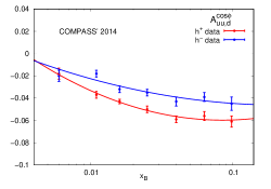
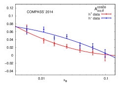
Figure 1: Smoothed functional fit to the ordinary asymmetries. $\chi^{2}_{d.o.f}=$ 0.49, 1.99, 0.47, and 1.56 for $A_{UU,d}^{\cos\phi,h^{+}}$, $A_{UU,d}^{\cos\phi,h^{-}}$, $A_{UU,d}^{\cos 2\phi,h^{+}}$ and $A_{UU,d}^{\cos 2\phi,h^{-}}$, respectively. Only statistical errors are shown.

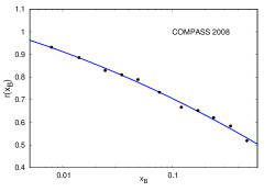
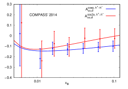
Figure 2: Left: smoothed functional fit for $r$ from COMPASS data Alekseev:2007vi . Right: for the difference asymmetries, Eq. (29). $\chi^{2}_{d.o.f}=$ 0.98 and 0.78 for $A_{UU,d}^{\cos\phi,h^{+}-h^{-}}$ and $A_{UU,d}^{\cos 2\phi,h^{+}-h^{-}}$, respectively. The points for $A_{UU,d}^{\cos 2\phi,h^{+}-h^{-}}$ are slightly shifted horizontally for better visibility. Combined statistical and systematic experimental errors are shown.

IV Numerical results on the BM function, $\langle k_{\perp}^{2}\rangle$ and $\langle p_{\perp}^{2}\rangle$

Here, we present the strategy of our analysis and the obtained results.

IV.1 Compatibility extraction of the Boer-Mulders function

We extract ${\cal N}_{{}_{B\!M}}(x_{{}_{\!B}})$ from relations (18) and (19) of the difference asymmetries . Relations (18) and (19) provide two independent equations for the extraction of ${\cal N}_{{}_{B\!M}}(x_{{}_{\!B}})$ for each set of the parameters in Table I. The analysis shows that the two extractions are compatible with each other, within errors, for the parameter values $\{\langle k_{\perp}^{2}\rangle,\;\langle p_{\perp}^{2}\rangle\}$,

$$\langle k_{\perp}^{2}\rangle=0.18\;{\rm GeV^{2}},\qquad\langle p_{\perp}^{2}\rangle=0.20\;{\rm GeV^{2}}$$ (31)

$$\langle k_{\perp}^{2}\rangle=0.25\;{\rm GeV^{2}},\qquad\langle p_{\perp}^{2}\rangle=0.20\;{\rm GeV^{2}},$$ (32)

with a slight preference for (32). Note that these values for $\langle k_{\perp}^{2}\rangle$ and $\langle p_{\perp}^{2}\rangle$ agree with those obtained in Giordano:2008th and with the theoretical considerations Zavada:2009ska ; Zavada:2011cv ; DAlesio:2009cps .

In Fig. 3, we present our results for Sets I, III, and V. The plots for Sets II and IV overlap with those for Sets I and III, respectively, which implies that our analysis is not sensitive to $M_{{}_{B\!M}}$. Consequently, in the following, we shall refer to Sets I, III, and V, only.
The excellent agreement with the data in Fig.3(b) suggests that the theoretical model, despite its simplifying assumptions, gives a realistic description of the Boer-Mulders function in the kinematic regime of the COMPASS experiment.

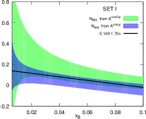
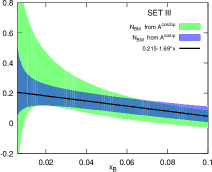
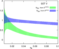
Figure 3: ${\cal N}_{{}_{B\!M}}^{Q_{V}}(x_{{}_{\!B}})$ extracted from the difference asymmetries, Eqs. (18) and (19), for Sets I, III, and V. Plots for Sets II and IV overlap with those for Sets I and III, respectively.

We obtain a simple linear fit to the extracted averaged ${\cal N}_{{}_{B\!M}}^{Q_{V}}$ for the parameter Set III, Eq. (32):

$${\cal N}_{{}_{B\!M}}^{Q_{V}}(x_{{}_{\!B}}) = ax_{{}_{\!B}}+b,$$

$$a=-1.69\pm 0.08,\quad b = 0.215\pm 0.006.$$ (33)

IV.2 Direct test for $\langle k_{\perp}^{2}\rangle$ and $\langle p_{\perp}^{2}\rangle$

Interestingly, there is a second way to utilize equations (18) and (19) which directly fixes the values of the parameters $\langle k_{\perp}^{2}\rangle,\,\langle p_{\perp}^{2}\rangle\,,M_{{}_{B\!M}}$, and $M_{{}_{C}}$ in Table I. Eliminating ${\cal N}_{{}_{B\!M}}^{Q_{V}}(x_{{}_{\!B}})$ from Eqs. (18) and (19) and using the variable $\rho$ we obtain,

$$A(x_{{}_{\!B}})=B(x_{{}_{\!B}}),$$ (34)

where

$$A(x_{{}_{\!B}}) \equiv \sqrt{\frac{\langle Q^{2}(x_{B})\rangle}{\langle k_{\perp}^{2}\rangle}}\,A_{UU,d}^{\cos\phi_{h},h^{+}-h^{-}}(x_{{}_{\!B}})\,+\rho\,A_{UU,d}^{\cos 2\phi_{h},h^{+}-h^{-}}(x_{{}_{\!B}}),$$ (35)

$$B(x_{{}_{\!B}}) \equiv {\cal C}_{Cahn}+\rho\,\frac{\langle k_{\perp}^{2}\rangle}{\langle Q^{2}(x_{B})\rangle}\,\hat{\cal C}_{Cahn}$$ (36)

and the explicit expression for $\rho$ is

$$\rho = \,-\frac{{\cal C}_{{}_{B\!M}}}{\hat{\cal C}_{{}_{B\!M}}}\,$$ (37)

$$= 2\,\frac{\int dz_{h}\,[\Delta^{N}D_{{q_{V}}\!\uparrow}^{h}(z_{h})]\,[\,z_{h}^{2}\lambda_{{}_{B\!M}}\,S_{3}(a,b,\langle P_{T}^{2}\rangle_{{}_{B\!M}})+\,(\eta\lambda_{{}_{C}}-z_{h}^{2}\lambda_{{}_{B\!M}})\,S_{1}(a,b;\langle P_{T}^{2}\rangle_{{}_{B\!M}})]/(z_{h}^{2}\lambda_{{}_{B\!M}}+\eta\lambda_{{}_{C}})^{3/2}}{\int dz_{h}\,[z_{h}\,\Delta^{N}D_{{q_{V}}\!\uparrow}^{h}(z_{h})]/(z_{h}^{2}\lambda_{{}_{B\!M}}+\eta\lambda_{{}_{C}})\,S_{2}(a,b;\langle P_{T}^{2}\rangle_{{}_{B\!M}})}$$

Figure 4 compares the two functions $A(x_{{}_{\!B}})$ and $B(x_{{}_{\!B}})$ for Sets I, III, and V.

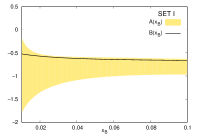
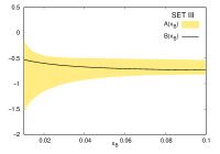
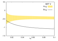
Figure 4: The test of Eq. (34) for Sets I, III, and V. Plots for Sets II and IV overlap with those for Sets I ($\chi^{2}_{d.o.f}=0.572$) and III ($\chi^{2}_{d.o.f}=0.151$), respectively.

One sees from Fig. 4 that the COMPASS data on $A_{UU}^{\cos\phi_{h}}$ and $A_{UU}^{\cos 2\phi_{h}}$, while roughly compatible with Set I again favour the parameter values of Set III, Eq. (32).

(Note that for calculating $\chi^{2}$ in Fig. 4 we use the COMPASS data points,

$$\chi^{2}=\sum_{i=1}^{N}\frac{\left(A(x_{i})-B(x_{i})\right)^{2}}{\left(\Delta A(x_{i})\right)^{2}}$$ (38)

divided by the degrees of freedom d.o.f= $N-l$, $l$ is the number of free parameters in the fit, in this fit $l=0$. Here $A(x_{i})$ and $B(x_{i})$ are values of the experimental points, $\Delta A(x_{i})$ are the errors at $x_{i}$ calculated from Eq. (30). In this way, we obtain $\chi^{2}$ for each of five sets in Table I testing which of them fits the data the best.) The compatibility of the two sides of Eq. (34) constitutes a further test of the simplifying assumptions made in our analysis.

V A word of caution: evolution, interaction terms, and higher twist

In the analysis above, as mentioned several times, we have not attempted to take into account any evolution in $Q^{2}$. As we shall explain, there are several reasons for this.

The mechanism of TMD evolution is formulated in terms of functions $\tilde{f}(x_{B},\bm{b}_{T},Q^{2})$ where $\bm{b}_{T}$ is the Fourier transform variable conjugate to $\bm{k}_{T}$,

$$f(x_{B},\bm{k}_{T},Q^{2})=\int\,d^{2}\,\bm{b}_{T}\,e^{i\bm{k}_{T}\cdot\bm{b}_{T}}\,\tilde{f}(x_{B},\bm{b}_{T},Q^{2})$$ (39)

The evolution between two values $Q_{0}$ and $Q$ is mainly controlled by a factor

$$\textrm{exp}\left\{\textrm{ln}\left(\frac{Q}{Q_{0}}\right)\,\tilde{K}(\bm{b}_{T},Q_{0})\right\}$$ (40)

where the Collins kernel $\tilde{K}(\bm{b}_{T},Q_{0})$ can be evaluated perturbatively only for small values of $b_{T}$. It is therefore split into a perturbative piece and a function $g_{K}(b_{T})$ representing the nonperturbative part, and which is determined from fitting experimental data.

It is generally agreed that at small $b_{T},\,g_{K}(b_{T})\propto b_{T}^{2}$, modulo a slowly varying logarithmic factor, but the expression

$$g_{K}(b_{T})=1/2\,g_{2}b_{T}^{2}$$ (41)

where $g_{2}$ is a parameter to be fixed from data, used in several papers for all $b_{T}$, is certainly incorrect at large $b_{T}$. In fact, Collins and Rogers Collins:2014jpa suggest that

$$g_{K}(b_{T})\xrightarrow{b_{T}\rightarrow\infty}\textrm{constant}.$$ (42)

It should be clear that generally the bigger the range of $Q^{2}$ covered by the data being fitted, the more accurate will be the determination of the function $g_{K}(b_{T})$. Consequently, the values of $g_{2}$ reported in the literature are heavily influenced by DY reactions and $Z$ production. Also, the shapes of the experimental distributions at large $Q^{2}$ suggest that the greatest sensitivity is to small values of $b_{T}$ and hence the extracted large $b_{T}$ behaviour could be quite misleading for the much lower $Q^{2}$ SIDIS reactions. A wide range of values for $g_{2}$ are given in the literature, varying from 0 to 0.90.
As an example, in an exploratory study, Anselmino et al. Anselmino:2012aa used the value $g_{2}=0.68$. But this implies that if a parton density has a width $\langle k_{\perp}^{2}\rangle\approx 0.20\,{\rm GeV^{2}}$ at $Q_{0}^{2}=1\,{\rm GeV^{2}}$, then at $Q^{2}=2.4\,{\rm GeV^{2}}$ the width has grown to $\langle k_{\perp}^{2}\rangle\approx 0.80\,{\rm GeV^{2}}$, surely a totally unphysical increase.
And in a later study focused on the SIDIS $Q^{2}$ range, Aidala et al. Aidala:2014hva suggested that $0\,\leq g_{2}\,\leq\,0.03$. The limited amount of data and the small range of $Q^{2}$ involved suggest that these measurements are not the most suitable for studying the structure of TMD evolution and we carried out our analysis ignoring TMD evolution. However, to give some feeling for possible evolution effects, in Fig. 5 we plot the function ${\cal N}_{{}_{B\!M}}^{Q_{V}}(x_{{}_{\!B}})$ taking into account evolution. We use the two extreme values $g_{2}=0$ (no evolution) and $g_{2}^{\rm{max}}$ up to which the evolution effects are negligible within experimental errors. We also present the results for $g_{2}=0.03$, given in Aidala:2014hva . We find $g_{2}^{\rm{max}}=0.05$ for the asymmetry $A^{\cos\phi}_{UU}$ and $g_{2}^{\rm{max}}=0.35$ for $A^{\cos 2\phi}_{UU}$.

Thus, in our analysis, we can neglect the evolution up to $g_{2}=0.05$, which is in agreement with Aidala:2014hva , keeping in mind all above comments.

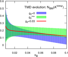
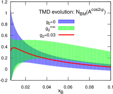
Figure 5: TMD evolution effects for the function ${\cal N}_{{}_{B\!M}}^{Q_{V}}(x_{{}_{\!B}})$ extracted from the difference asymmetries, Eqs. (18) and (19), for Set III (the same occurs also for other parameter sets). We show results obtained using the two extreme values $g_{2}=0$ (no evolution) and $g_{2}=g_{2}^{\rm{max}}$ up to which the evolution effects are negligible within experimental errors, the solid line shows ${\cal N}_{{}_{B\!M}}^{Q_{V}}(x_{{}_{\!B}})$ for $g_{2}=0.03$, given in Aidala:2014hva .

The expression Eq. (18), which we have used above for the asymmetry $A_{UU}^{\cos\phi_{h},h-\bar{h}}(x_{{}_{\!B}})$, is incomplete. There are so called interaction-dependent terms Bacchetta:2006tn , linked to the quark-gluon-quark correlators, which have been left out. These interaction terms are unknown, but we might expect to have roughly

$$|\textrm{Interaction-dependent terms}|\sim\alpha_{s}|\textrm{terms in }\textrm{Eq.}~{}(\ref{A1})|.$$ (43)

In our kinematic range, the average value of $\alpha_{s}$ is approximately $0.35$, which suggests that such terms might be small compared to the terms kept in Eq. (18). Attempts have been made in the literature to estimate the size of terms of this type, at least where they occur in the difference between the true value of the structure function $g_{T}$ and the Wandzura-Wilczek (WW) approximation $g_{T}^{WW}$ to it. The data on $g_{T}$ were compared with $g_{T}^{WW}$ by Accardi et al. Accardi:2009au , who claimed differences of order $15\%-35\%$. However, the data are of very poor quality so that the conclusion reached in Accardi:2009au does not seem convincing. On the other hand, a recent lattice calculation of $g_{T}$ by Bhattacharya et al. Bhattacharya:2020cen found very good agreement with $g_{T}^{WW}$ out to $x_{B}=0.4$. In any event, the terms neglected in the WW approximation to $g_{T}$ are not the same as those ignored in the $\cos\phi_{h}$ asymmetry, so these results can only be considered as a hint that the terms ignored in the $\cos\phi_{h}$ asymmetry are indeed negligible.
It should be noted that in their recent general study of asymmetries in SIDIS, in the section on $\cos 2\phi_{h}$ and $\cos\phi_{h}$ asymmetries, Bastami et al. Bastami:2018xqd found significant differences between the $\cos\phi_{h}$ asymmetry data and what they refer to as the WW approximation to it. However, Bastami et al. Bastami:2018xqd utilized the results of Barone:2009hw ; Barone:2010gk , which, as the present study demonstrates, are incorrect.

Ultimately, the excellent fit to the data found in this study, together with the successful consistency test, suggests that the omission of these terms is justified.

Finally, it should be noted that the expression Eq. (19) for the asymmetry $A_{UU}^{\cos 2\phi_{h},h-\bar{h}}(x_{{}_{\!B}})$ is unusual in that it contains a combination of a twist-2 BM term ${\cal N}_{{}_{B\!M}}^{Q_{V}}(x_{{}_{\!B}})\,\hat{\cal C}_{{}_{B\!M}}^{h}$ with a twist-4 Cahn term $\langle k_{\perp}^{2}\rangle/\langle Q^{2}\rangle\,\cdot\,\hat{\cal C}^{h}_{Cahn}$, and one might wonder whether there might exist important twist-4 BM terms which are not accounted for in Eq. (19). That this is not so can be understood from the following argument. In Fig. 6, we compare the BM and Cahn contributions to Eq. (19). Remarkably, the twist-4 Cahn term contribution is not negligibly small in magnitude compared to the twist-2 BM contribution! This peculiar situation is due to two factors. First, the twist-4 prefactor in the Cahn term, $\langle k_{\perp}^{2}\rangle/\langle Q^{2}\rangle$, is not really small for the values of $Q^{2}$ in our data. Second, the Cahn factor $\hat{\cal C}^{h}_{Cahn}$ is anomalously large because it depends on the unpolarized PDFs and FFs. This suggests that any further twist-4 BM type contribution would be expected to be negligibly small by comparison and it also explains our earlier comment that the neglect of this Cahn term in Barone:2015ksa is dangerous and unjustified.

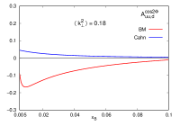
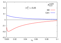
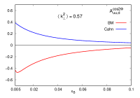
Figure 6: Comparison of the BM with Cahn contribution to the $\cos 2\phi_{h}$ asymmetry for $\langle k_{\perp}^{2}\rangle=0.18$ (left), $\langle k_{\perp}^{2}\rangle=0.25$ (middle), and $\langle k_{\perp}^{2}\rangle=0.57\,{\rm GeV^{2}}$ (right).

VI Comparison to other Boer-Mulders parametrizations

Our valence Boer-Mulders function $\Delta f_{{}_{B\!M}}^{Q_{V}}(x_{{}_{\!B}})$,

$$\Delta f^{Q_{V}}_{{}_{B\!M}}(x_{{}_{\!B}},Q^{2})\!=\!2\,{\cal N}_{{}_{B\!M}}^{Q_{V}}(x_{{}_{\!B}})\,Q_{V}(x_{{}_{\!B}},Q^{2})\,,$$ (44)

is shown in Fig. 7, where it is compared to $\Delta f_{{}_{B\!M}}^{Q_{V}}(x_{{}_{\!B}})$ calculated using two other parametrizations of BM functions available in literature–the BM functions published in Barone:2009hw ; Barone:2010gk and in Zhang:2008nu ; Lu:2009ip . The BM function published in Barone:2009hw ; Barone:2010gk is extracted from the $\cos 2\phi_{h}$ asymmetry in SIDIS, using the simplifying, but theoretically inconsistent, assumption that it is proportional to the Sivers function for each quark flavour separately. The parametrizations in Zhang:2008nu ; Lu:2009ip are extracted from the azimuthal $\cos 2\phi_{h}$ asymmetry of the final lepton pair in unpolarized Drell-Yan processes. We compare our result to the parametrization in Lu:2009ip , obtained from the combined analysis of the $pp$ and $pd$ DY processes.

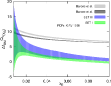
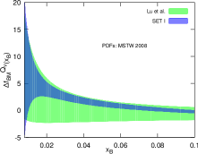
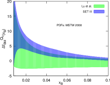
Figure 7: Comparison of $\Delta f_{{}_{B\!M}}^{Q_{V}}$ for Sets I and III with the result of Barone et al. (left) Barone:2009hw (light gray) and Barone:2010gk (dark gray) and with Lu and Schmidt Lu:2009ip –middle (Set I) and right (Set III). We use, respectively, GRV1998 Gluck:1998xa and MSTW2008 Martin:2009iq parametrizations for the collinear PDFs.

It is seen that, both for Sets I and III, there is a significant difference between our predictions and those of Refs. Barone:2009hw ; Barone:2010gk , and a good agreement with the results in Lu:2009ip from DY data. This suggests that the BM functions in Barone:2009hw ; Barone:2010gk are incorrect.

VII Test of the Boer-Mulders to Sivers relation

In Refs. Barone:2008tn ; Barone:2009hw ; Barone:2010gk , the BM functions were assumed proportional to the Sivers functions for each quark and antiquark flavour $q$ separately,

$$\Delta f^{q}_{{}_{B\!M}}(x_{{}_{\!B}},k_{\perp})=\lambda_{q}\,\Delta f^{q}_{Siv}(x_{{}_{\!B}},k_{\perp}),$$ (45)

which, as implied by the results in Fig. 7 above, is badly violated, in agreement with conclusions reached in our earlier paper Christova:2015jsa . We here return to the question of the proportionality between the BM and Sivers functions, but now only for the valence-quark contributions $Q_{V}=u_{V}+d_{V}$,

$$\Delta f^{Q_{V}}_{{}_{B\!M}}(x_{{}_{\!B}},k_{\perp})=\lambda\,\Delta f^{Q_{V}}_{Siv}(x_{{}_{\!B}},k_{\perp})$$ (46)

For the Sivers function we use an analogous parametrization to the BM, Eq. (6), but with the replacements $M_{{}_{B\!M}}\to M_{{}_{S}}$ and ${\cal N}_{{}_{B\!M}}\to{\cal N}_{Siv}$. Then, Eq. (46) implies $M_{{}_{B\!M}}=M_{{}_{S}}$, and

$${\cal N}_{{}_{B\!M}}^{Q_{V}}(x_{{}_{\!B}})=\lambda\,\,{\cal N}_{Siv}^{Q_{V}}(x_{{}_{\!B}})$$ (47)

which we shall now test.

We extract ${\cal N}_{Siv}(x_{{}_{\!B}})$ from the difference Sivers asymmetries $A_{UT}^{Siv,h^{+}-h^{-}}(x_{{}_{\!B}})$ using the single-spin asymmetries presented by COMPASS for $h^{\pm}$ on deuterons Alekseev:2008aa . The expression for $A_{UT}^{Siv,h^{+}-h^{-}}(x_{{}_{\!B}})$ is Christova:2015jsa

$$A_{UT,d}^{Siv,h^{+}-h^{-}}(x_{{}_{\!B}}) = \sqrt{\frac{e\pi}{2}}\,\,K_{Siv}^{h}\,{\cal N}_{Siv}^{Q_{V}}(x_{{}_{\!B}}),$$ (48)

$$K_{Siv}^{h}=\frac{\langle k_{\perp}^{2}\rangle_{{}_{S}}^{2}}{M_{{}_{S}}\langle k_{\perp}^{2}\rangle}\,\frac{\int dz_{h}\,z_{h}[D_{q_{V}}^{h}]/\sqrt{\langle P_{T}^{2}\rangle_{{}_{S}}}}{\int dz_{h}\,[D_{q_{V}}^{h}]},\quad\langle P_{T}^{2}\rangle_{{}_{S}}=\langle p_{\perp}^{2}\rangle+z_{h}^{2}\langle k_{\perp}^{2}\rangle_{{}_{S}}$$ (49)

In Fig.8, we show the measured single-spin $A_{Siv}^{h^{\pm}}$ and difference $A_{Siv}^{h^{+}-h^{-}}$ Sivers asymmetries, and in Fig.9, we show the extracted BM and Sivers functions ${\cal N}_{{}_{B\!M}}^{Q_{V}}(x_{{}_{\!B}})$ and ${\cal N}_{Siv}^{Q_{V}}(x_{{}_{\!B}})$ for Sets I and III. We see that Eq. (47) holds fairly well, confirming the results of Christova:2015jsa , and that $\lambda\approx 1.0$ for both Set I and Set III.

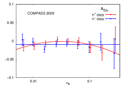
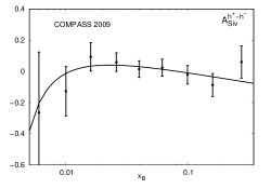
Figure 8: Smooth fits to the Sivers asymmetries: $A_{Siv}^{h^{\pm}}$ (left) and $A_{Siv}^{h^{+}-h^{-}}$ (right).

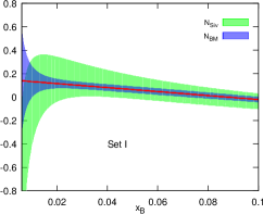
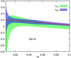
Figure 9: Test of proportionality for BM to Sivers functions, Eq. (47). Both for Set I (left) and Set III (right), ${\cal N}_{{}_{B\!M}}^{Q_{V}}(x_{{}_{\!B}})$ overlaps ${\cal N}_{Siv}^{Q_{V}}(x_{{}_{\!B}})$, which implies $\lambda\approx 1$ for both sets.

VIII Conclusions

In a combined analysis of the $\cos\phi_{h}$ and $\cos 2\phi_{h}$ azimuthal asymmetries in unpolarized SIDIS, measured most recently by COMPASS, we determined (1) the BM function $f^{Q_{V}}_{{}_{B\!M}}(x_{{}_{\!B}},Q^{2})$ for the sum of the valence quarks $Q_{V}=u_{V}+d_{V}$ and (2) obtained information on the average transverse momenta $\langle k_{\perp}^{2}\rangle$ and $\langle p_{\perp}^{2}\rangle$, which play a role in the transverse momentum dependent parton distribution functions and fragmentation functions, respectively. The analysis is based on a study of the so-called difference asymmetries between hadron $h$ and $\bar{h}$. The results are obtained using the often made simplifying assumption of factorization of transverse momentum and $x_{B}$ dependence, with the transverse momentum behaviour given by Gaussians, with $x_{{}_{\!B}}$-independent widths. The excellent agreement with the data, as well as the positive result of the compatibility test, Sec. (IV.2), suggests that these simplifications are valid in the kinematic region of the COMPASS experiment.
We have compared our results to the existing ones in the literature. For the BM function, we agree with the results obtained from an analysis of DY processes Zhang:2008nu ; Lu:2009ip but disagree strongly with the results obtained in a model analysis of the $\cos 2\phi_{h}$ asymmetry in SIDIS in Barone:2009hw ; Barone:2010gk , both obtained under the same simplifying assumptions as in this paper. It should be noted that in their recent general study of asymmetries in SIDIS, in the section on $\cos 2\phi_{h}$ and $\cos\phi_{h}$ asymmetries, Bastami et al. Bastami:2018xqd utilized the, according to our study, unreliable results of Barone:2009hw ; Barone:2010gk .
Our favoured values for $\langle k_{\perp}^{2}\rangle$ and $\langle p_{\perp}^{2}\rangle$ agree with those obtained in a previous analysis of the $\cos\phi_{h}$ and $\cos 2\phi_{h}$ modulations in SIDIS, Anselmino:2005nn ; Giordano:2008th , i.e., ($\langle k_{\perp}^{2}\rangle=0.18\;{\rm GeV^{2}};\langle p_{\perp}^{2}\rangle=0.20\;{\rm GeV^{2}}$) and ($\langle k_{\perp}^{2}\rangle=0.25\;{\rm GeV^{2}};\langle p_{\perp}^{2}\rangle=0.20\;{\rm GeV^{2}}$), and disagree with the later, larger values ($\langle k_{\perp}^{2}\rangle=0.57\,{\rm GeV^{2}};\langle p_{\perp}^{2}\rangle=0.12\,{\rm GeV^{2}}$) obtained from a study of multiplicities Anselmino:2013lza .
Finally, we note that future data on the $\langle\cos\phi_{h}\rangle$ and $\langle\cos 2\phi_{h}\rangle$ asymmetries on protons, for charged pions or kaons, will allow access to the BM function for the valence quarks $u_{V}$ and $d_{V}$ separately, in the same, approximately model-independent manner Christova:2015jsa .

IX Acknowledgements

E. C. and D. K. acknowledge the support of the INRNE-BAS (Bulgaria)-JINR (Russia) collaborative grant. E. C. is grateful to Grant No. 08-17/2016 of the Bulgarian Science Foundation and D. K. acknowledges the support of the Bogoliubov-Infeld Program. D. K. also thanks A. Kotlorz for useful comments on numerical analysis.

References

- (1) D. Boer and P. J. Mulders, Phys. Rev. D 57, 5780 (1998), hep-ph/9711485.
- (2) V. Barone, A. Prokudin, and B.-Q. Ma, Phys. Rev. D 78, 045022 (2008), arXiv:0804.3024.
- (3) V. Barone, S. Melis, and A. Prokudin, Phys. Rev. D 81, 114026 (2010), arXiv:0912.5194.
- (4) V. Barone, S. Melis, and A. Prokudin, Phys. Rev. D 82, 114025 (2010), arXiv:1009.3423.
- (5) A. Bacchetta, F. Conti, and M. Radici, Phys. Rev. D 78 074010 (2008), arXiv:0807.0323.
- (6) A. Courtoy, S. Scopetta, and V. Vento, Phys. Rev. D 80, 074032 (2009), arXiv:0909.1404.
- (7) B. Pasquini and F. Yuan, Phys. Rev. D 81, 114013 (2010), arXiv:1001.5398.
- (8) E. Christova, E. Leader, and M. Stoilov, Phys. Rev. D 97, 056018 (2018), arXiv:1705.10613.
- (9) E. Christova, D. Kotlorz, and E. Leader, arXiv:1909.08218.
- (10) B. Zhang, Z. Lu, B.-Q. Ma, and I. Schmidt, Phys. Rev. D 77, 054011 (2008), arXiv:0803.1692.
- (11) Z. Lu and, I. Schmidt, Phys. Rev. D 81, 034023 (2010), arXiv:0912.2031.
- (12) X. Wang, W. Mao, and Z. Lu, Eur. Phys. J. C 78, 643 (2018), arXiv:1805.03017.
- (13) E. Christova and E. Leader, Nucl. Phys. B607, 369 (2001), hep-ph/0007303.
- (14) E. Christova and E. Leader, Phys. Rev. D 92, 114004 (2015), arXiv:1507.01399.
- (15) E. Christova, Phys. Rev. D 90 054005 (2014); arXiv:1407.5872
- (16) C. Adolph et al. (COMPASS Collaboration), Nucl. Phys. B886, 1046 (2014), arXiv:1401.6284.
- (17) A. Bacchetta, F. Delcarro, C. Pisano, M. Radici, and A. Signori, J. High Energy Phys. 06 (2017) 081; (2019) 051(E), arXiv:1703.10157.
- (18) A. Bacchetta V. Bertone, C. Bissolotti, G. Bozzi, F. Delcarro, F. Piacenza, and M. Radici, arXiv:1912.07550.
- (19) I. Scimemi and A. Vladimirov, Eur. Phys. J. C 78, 89 (2018), arXiv:1706.01473.
- (20) I. Scimemi and A. Vladimirov, J. High Energy Phys. 06 (2020) 137, arXiv:1912.06532.
- (21) A. Signori, A. Bacchetta, M. Radici, and G. Schnell, J. High Energy Phys. 11 (2013) 194, arXiv:1309.3507.
- (22) M. Anselmino, M. Boglione, and S. Melis, Phys. Rev. D 86, 014028 (2012), arXiv:1204.1239.
- (23) V. Bertone, I. Scimemi, and A. Vladimirov, J. High Energy Phys. 06 (2019) 028, arXiv:1902.08474.
- (24) M. Anselmino, M. Boglione, U. D’Alesio, S. Melis, F. Murgia, E. R. Nocera, and A. Prokudin, Phys. Rev. D 83, 114019 (2011), arXiv:1101.1011.
- (25) J. C. Collins, Nucl. Phys. B396, 161 (1993), hep-ph/9208213.
- (26) M. Anselmino, M. Boglione, U. D’Alesio, A. Kotzinian, F. Murgia, A. Prokudin, and S. Melis, Nucl. Phys. B Proc. Suppl. 191, 98 (2009), arXiv:0812.4366.
- (27) M. Anselmino, M. Boglione, U. D’Alesio, J. O. Gonzalez Hernandez, S. Melis, F. Murgia, and A. Prokudin, Phys. Rev. D 92, 114023 (2015), arXiv:1510.05389.
- (28) M. Anselmino, M. Boglione, U. D’Alesio, J. O. Gonzalez Hernandez, S. Melis, F. Murgia, and A. Prokudin, Phys. Rev. D 93, 034025 (2016), arXiv:1512.02252.
- (29) R. N. Cahn, Phys. Lett. 78B, 269 (1978).
- (30) R. N. Cahn, Phys. Rev. D 40, 3107 (1989).
- (31) Al. Bacchetta, M. Diehl, K. Goeke, A. Metz, P. J. Mulders, and M. Schlegel, J. High Energy Phys. 02 (2007) 093, hep-ph/0611265.
- (32) V. Barone, M. Boglione, J. O. Gonzalez Hernandez, and S. Melis, Phys. Rev. D 91, 074019 (2015), arXiv:1502.04214.
- (33) U. D’Alesio and F. Murgia, Prog. Part. Nucl. Phys. 61, 394 (2008), arXiv:0712.4328.
- (34) F. Bradamante, AIP Conf. Proc. 915, 513 (2007), hep-ex/0702007.
- (35) M. Anselmino, M. Boglione, U. D’Alesio, A. Kotzinian, F. Murgia, and A. Prokudin, Phys. Rev. D 71, 074006 (2005), hep-ph/0501196.
- (36) M. Arneodo et al. (EMC Collaboration), Z. Phys. C 34, 277 (1987).
- (37) M. R. Adams et al. (Fermilab E665 Collaboration), Phys. Rev. D 48, 5057 (1993).
- (38) F. Giordano, DESY Report No. DESY-THESIS-2008-030.
- (39) M. Anselmino, M. Boglione, J. O, Gonzalez Hernandez, S. Melis, and A. Prokudin, J. High Energy Phys. 04 (2014) 005, arXiv:1312.6261.
- (40) A. Airapetian et al. (HERMES Collaboration), Phys. Rev. D 87, 074029 (2013), arXiv:1212.5407.
- (41) C. Adolph et al. (COMPASS Collaboration), Eur. Phys. J. C 73, 2531 (2013), arXiv:1305.7317.
- (42) M. Anselmino, M. Boglione, U. D’Alesio, F. Murgia, and A. Prokudin, Phys. Rev. D 98, 094023 (2018), arXiv:1809.09500.
- (43) M. Anselmino, M. Boglione, U. D’Alesio, A. Kotzinian, S. Melis, F. Murgia, A. Prokudin and C. Turk, Eur. Phys. J. A 39, 89 (2009), arXiv:0805.2677.
- (44) M. Anselmino, M. Boglione, U. D’Alesio, F. Murgia, and A. Prokudin, J. High Energy Phys. 04 (2017) 046, arXiv:1612.06413.
- (45) M. Anselmino, M. Boglione, U. D’Alesio, A. Kotzinian, F. Murgia, A. Prokudin, and C. Turk, Phys. Rev. D 75, 054032 (2007), hep-ph/0701006.
- (46) M. Anselmino, M. Boglione, U. D’Alesio, S. Melis, F. Murgia, and A. Prokudin, in Proceedings of the XIX International Workshop on Deep Inelastic Scattering and Related Subjects (DIS 2011), April 11-15, 2011 (Newport News, VA, 2011), arXiv:1107.4446.
- (47) M. Alekseev et al. (COMPASS Collaboration), Phys. Lett. B 673 127 (2009), arXiv:0802.2160.
- (48) S. Albino, B.A. Kniehl, and G. Kramer, Nucl. Phys. B803, 42 (2008), arXiv:0803.2768
- (49) M. Alekseev et al. (COMPASS Collaboration), Phys. Lett B 660, 458 (2008), arXiv:0707.4077.
- (50) P. Zavada, Phys. Rev. D 83, 014022 (2011), arXiv:0908.2316.
- (51) P. Zavada, Phys. Rev. D 85, 037501 (2012), arXiv:1106.5607.
- (52) U. D’Alesio, E. Leader, and F. Murgia, Phys. Rev. D 81, 036010 (2010), arXiv:0909.5650.
- (53) J. Collins and T. Rogers, Phys. Rev. D 91, 074020 (2015), arXiv:1412.3820.
- (54) C. Aidala, B. Field, L. Gamberg, and T. Rogers, Phys. Rev. D 89, 094002 (2014), arXiv:1401.2654.
- (55) A. Accardi, A. Bacchetta, W. Melnitchouk, and M. Schlegel, J. High Energy Phys. 11 (2009) 093, arXiv:0907.2942.
- (56) S. Bhattacharya, K. Cichy, M. Constantinou, A. Metz, A. Scapellato, and F. Steffens, arXiv:2004.04130.
- (57) S. Bastami et al., J. High Energy Phys. 06 (2019) 007, arXiv:1807.10606.
- (58) M. Glück, E. Reya, and A. Vogt, Eur. Phys. J. C 5, 461 (1998), hep-ph/9806404.
- (59) A. D. Martin, W. J. Stirling, R. S. Thorne, and G. Watt, Eur. Phys. J. C 63, 189 (2009), arXiv:0901.0002.