Event Clustering & Event Series Characterization on Expected Frequency

Abstract

We present an efficient clustering algorithm applicable to one-dimensional data such as e.g. a series of timestamps. Given an expected frequency $\Delta T^{-1}$, we introduce an $\mathcal{O}(N)$–efficient method of characterizing $N$ events represented by an ordered series of timestamps $t_{1},t_{2},\dots,t_{N}$. In practice, the method proves useful to e.g. identify time intervals of missing data or to locate isolated events. Moreover, we define measures to quantify a series of events by varying $\Delta T$ to e.g. determine the quality of an Internet of Things service.

I Motivation

The concept of Internet of Things (IoT) [1, 2] is intimately related to records of certain events, e.g. a network attached device capturing weather information to be broadcasted to other devices for processing. Given a) the transmitter frequently sends out such information every time interval $\Delta T$, and b) the receiving device keeps track of the timestamps when data was transmitted/recorded, the time series $t=\{t_{i}\}_{i=1\dots N}$ stores information on failure of recording/sending/transmission/receiving.

If we cluster the one-dimensional data $t$ such that consecutive events are not more than $\Delta T$ apart, we can infer periods in time where data might be missing. Upon detection, corresponding action such as retransmission, data interpolation, etc. can be performed. Moreover, the characteristics of intervals of no data (relative frequency, duration, …) might help to diagnose the sanity of the communication network.

Since general purpose, multi-dimensional clustering methods such as Fisher’s discriminant [3], k–means [4] or more generally EM [5] do not exploit the special property of ordering in one dimension, we aim at a simpler approach that does not need knowledge of the number of clusters/intervals, and it avoids density estimation such as with denclue [6].

Regarding cluster classification our approach is close to the conceputal notion dbscan [7] introduces: clusters of points and outliers/noise points. However, we exploit the fact that the sequence of timestamps is naturally ordered and thus minimize computational complexity by a factor of $\mathcal{O}(\log N)$. Of course, if we would have to sort $t$ first, e.g. using heapsort [8], we are back to asymptotic runtime of $\mathcal{O}(N\log N)$.

Our main contribution here is to adapt the concept of dbscan to event clustering for application in IoT service quality characterization. We present an algorithm with linear runtime complexity which asymptotically outperforms native dbscan that operates at an overall average runtime complexity of $\mathcal{O}(N\log N)$. Of course, while dbscan can be applied to any number of spatial dimensions our approach is limited to the one-dimensional case.

II One-Dimensional Clustering

II-A Problem Formulation

Given a set of $N$ ordered timestamps $t=\{t_{i}\}_{i=1\dots N}$, i.e.

$$i\leq j\quad\Rightarrow\quad t_{i}\leq t_{j}$$ (1)

and an expected time interval $\Delta T$, provide time intervals $\tau_{k}$ such that

$$t_{i},t_{i+1}\in\tau_{k}=[\tau_{k}^{-},\tau_{k}^{+}]\quad\Rightarrow\quad\delta t_{i}=t_{i+1}-t_{i}\leq\Delta T\quad.$$ (2)

Note that $\Delta T$ might be an external parameter to the algorithm that provides the solution or it is defined by $t$ itself, e.g. through $\langle\delta t\rangle=\tfrac{1}{N}\sum_{i}\delta t_{i}$. As we will discuss, the $\delta t_{i}$ need to be computed and therefore $\langle\delta t\rangle$ is efficiently determined along the lines.

II-B Central Idea

In order to fulfill eq. 2, of course, we need to compute at least $N-1$ time intervals

$$\delta t=\{\delta t_{i}=t_{i+1}-t_{i}\}_{i=1\dots N-1}\quad.$$ (3)

Whenever a new time series point $t_{N+1}>t_{N}$ gets (randomly) added, there is no a priory way of determining whether $\Delta T$ got exceeded from the existing $t_{i\leq N}$.

To classify the $t_{i}$ as interval bounds $\tau^{\pm}_{k}$ we note that the binary sequence

$$b=\{b_{i}=int(\delta t_{i}>\Delta T)\}_{i=1\dots N-1}$$ (4)

switches from 1 to 0 for an opening interval bound $\tau^{-}$, and from 0 to 1 for a closing interval bound $\tau^{+}$, only. $int(\cdot)$ denotes the function $int(True)\to 1$ and $int(False)\to 0$. Hence the quantity

$$B=\{B_{i}=b_{i}-b_{i-1}\}_{i=2\dots N-1}\quad\text{with}\quad B_{i}\in\{-1,0,1\}$$ (5)

yields the desired association

$$B_{i}=\pm 1\quad\Rightarrow\quad t_{i}\in\tau^{\pm}\quad.$$ (6)

Per requirement, a) eq. 1, the $t_{i}$ are ordered, and b) the binary (discrete) function $b_{i}$ implies the alternating property

$$\forall i<j:~{}~{}1=B_{i}=B_{j}\quad\Rightarrow\quad\exists i<l<j:~{}~{}B_{l}=-1\quad.$$ (7)

Thus, linearly scanning through the $t_{i}$ and their corresponding $B_{i}$ results in the two sets

$$\tau^{\pm} =\{\tau^{\pm}_{k}:k<k^{\prime}\Rightarrow\tau^{\pm}_{k}<\tau^{\pm}_{k^{\prime}}\}_{k=1\dots K^{\pm}\leq N/2-1}$$ (8)

such that we can simply interleave these to obtain the corresponding time intervals as our solution, eq. 2.

II-C Boundary Conditions

However, there is a couple of options how to exactly interleave the $\tau^{\pm}$ which depend on the boundary condition. More specifically, let us assume the sequence $t_{1},t_{2},\dots$ starts e.g. with intervals that are smaller than $\Delta T$. In this case, $\tau^{-}_{1}>\tau^{+}_{1}$, and one needs to manually add a $\tau^{-}_{0}$ to construct intervals

$$\tau_{k}=[\tau^{-}_{k-1},\tau^{+}_{k}]\quad.$$ (9)

A corresponding issue might happen at the end of the time series $\{t_{i}\}$ depending on whether $K^{+}=\left|\tau^{+}\right|$ is equal or not equal to $K^{-}=\left|\tau^{-}\right|$.

⬇

1algorithm cluster_events is

2 input: list t of ordered timestamps $t$,

3 float variable dT of expected inverse frequency $\Delta T$

4 output: list tau of cluster intervals $\tau$,

5 list x of isolated timestamps $x$

6

7 define lists tauMinus, tauPlus, tau, x

8 define lists dt, b, B

9

10 N $\leftarrow$ length of t

11 b[0] $\leftarrow$ 1

12 b[N] $\leftarrow$ 1

13

14 for each i in 1,2,…,N-1 do

15 dt[i] $\leftarrow$ t[i] - t[i-1]

16 if dt[i] $>$ dT then b[i] $\leftarrow$ 1

17 else b[i] $\leftarrow$ 0

18

19 for each i in 0,1,…,N-1 do

20 B[i] $\leftarrow$ b[i+1] - b[i]

21 if B[i] = -1 then append t[i] to tauMinus else

22 if B[i] = 1 then append t[i] to tauPlus else

23 if b[i+1] = 1 then append t[i] to x

24

25 for each i in 0,…,length of tauMinus do

26 add interval [tauMinus[i], tauPlus[i]] to tau

27

28 return tau, x

Listing 1: Sample implementation of our clustering procedure as pseudo-code.

In order to prevent manually dealing with all the (four) different boundary condition scenarios, we might want to (virtually) add the following timestamps from the outset:

$$t_{0}=-\infty\quad\text{and}\quad t_{N+1}=+\infty\quad.$$ (10)

Hence, we obtain $\delta t_{0}=\delta t_{N}=+\infty$, and therefore

$$b_{0}=b_{N}=1$$ (11)

which yields $N$ $B_{i}$ that corresponding to $N$ $t_{i}$ for classification such that we always have

$$\tau=\left\{\tau_{k}=[\tau^{-}_{k},\tau^{+}_{k}]\right\}_{k=1\dots K}$$ (12)

from

$$\tau^{\pm} =\left\{\tau^{\pm}_{k}:k<k^{\prime}\Rightarrow\tau^{\pm}_{k}<\tau^{\pm}_{k^{\prime}}\right\}_{k=1\dots K}$$ (13)

with $|\tau|=K\leq N/2$.

II-D Isolated Points

Given the solution eq. 12, due to the ordering of the $t_{i}$, we can simply form the open intervals

$$\bar{\tau}=\left\{\bar{\tau}_{k}=\left(\tau^{+}_{k},\tau^{-}_{k+1}\right)\right\}_{k=1\dots K-1}$$ (14)

that we associate with time intervals of failure. Note, that $[t_{1},t_{N}]=\tau\cup\bar{\tau}$. However, these intervals do not imply

$$\forall i,k:t_{i}\notin\bar{\tau}_{k}$$ (15)

i.e., informally, it is not true that no event happens during the intervals $\bar{\tau}$, but we certainly have

$$t_{i}\in\bar{\tau}_{k}\quad\Rightarrow\quad|t_{i}-t_{i\pm 1}|>\Delta T$$ (16)

where we refer to $t_{i}$ as an isolated event. In terms of dbscan these timestamps form the noise, while all $t_{i}\in\tau^{\pm}$ are border points.

Isolated events have $b_{i}=1$ and since they are not interval boundary points they need to have $B_{i}=0$. This way we can use $b$ and $B$ to classify isolated events according to

$$B_{i}=0\wedge b_{i}=1\quad\Rightarrow\quad t_{i}\in x$$ (17)

where $x$ denotes the set of isolated timestamps. Likewise, we can define clustered timestamps as

$$B_{i}=0\wedge b_{i}=0\quad\Rightarrow\quad t_{i}\in\bar{x}\quad.$$ (18)

Since $b$ is binary and eq. 5 holds for $B$, all $t_{i}$ are uniquely classified, i.e. $t=\tau^{+}\cup\tau^{-}\cup x\cup\bar{x}$. It is rather straightforward to convince oneself that there is the association $\stackrel{{\scriptstyle(-)}}{{x}}\leftrightarrow\stackrel{{\scriptstyle(-)}}{{\tau}}$ in the sense that all $t_{i}\in x$ are within an interval of $\bar{\tau}$ and $t_{i}\in\bar{x}$ within an interval of $\tau$.

II-E Implementation & Computational Complexity

LABEL:lst:PseudoCodeImpl provides an example implementation of the method from sections II-B and II-C in pseudo-code for demonstration purposes. E.g. the call of cluster_events(t, dT) on

t=[-20,-18,1,2,2.9,10,11,100,200,202,202,203]

given dT as

-1, 0, 1, 10, 100, and mean of the elements of t

returns output equivalent to
 [], [-20, -18, 1, 2, 2.9, 10, 11, 100, 200, 202, 202, 203]
 [[202, 202]], [-20, -18, 1, 2, 2.9, 10, 11, 100, 200, 203]
 [(1, 2.9), (10, 11), (202, 203)], [-20, -18, 100, 200]
 [(-20, -18), (1, 11), (200, 203)], [100]
 [(-20, 203)], []
 [(-20, 11), (200, 203)], [100]
respectively.

The procedure presented in sections II-B, II-C and II-D and LABEL:lst:PseudoCodeImpl uses $N-1$ algebraic operations for $\delta t$, $N-2$ logical operations for $b$ and again $N$ algebraic operations for $B$ which determines the interval boundary classification with a total of $3(N-1)$ operations. The final loop in LABEL:lst:PseudoCodeImpl to interleave the tauPlus and tauMinus lists is just for the user’s convenience.

The naive approach would compute two time intervals for each $t_{i}$ and perform two logical operations of those against $\Delta T$ to determine the classification, hence $4N$ computations. Note that due to the given linear ordering in one-dimensional space, our algorithm’s runtime $3N-3$ is exact. In particular, it is fully deterministic when the number of timestamps $N$ is fixed.

Moreover, the required memory for our approach is linear in $N$. Only the event series list t of size $N$ and the lists x, tauMinus, and tauPlus with a total size of at most $N$ timestamps need to be stored. The lists dt, b, and B can be computed on the fly occupying storage $\mathcal{O}(1)$.

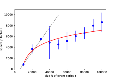
Figure 1: Numerical speedup analysis comparing a Python implementation of our algorithm using the module numpy [9], v1.13.0, to the vanilla implementation of dbscan, DBSCAN(), from the package sklearn [10], v0.18.1, module cluster with parameter settings min_samples=2 and metric=’l1’. We plot the quantity $r$ (cf. blue dots) from eq. 19 versus the number of timestamps $N=|t|$ to cluster.
Timing measurements were performed with the standard Python module timeit on commodity hardware with sufficient RAM to prevent swapping. Experiments have been repeated 40 times to aggregate statistics for error estimation using error propagation by first order Taylor expansion.
The event series was generated by a white noise random distribution on $[0,1)$ and has been rescaled by $N$. For the experiments, dT was set to two values: 1 and 1e-4, corresponding to the parameter eps of DBSCAN().
While we observed an approximately linear speedup for small $N$ (cf. gray, dashed fit line $a\cdot r+b$), an overall logarithmic speedup (cf. red, solid fit line $c\log[a\cdot r+b]$) is plausible which supports the analytical result: $\mathcal{O}(N\log N)/\mathcal{O}(N)=\mathcal{O}(\log N)$.

To confirm our analytical findings we performed a numerical experiment which is presented by fig. 1. It evaluates the speedup of our algorithm compared to a vanilla implementation of dbscan. Within the observed error boundaries, the scaling factor $\mathcal{O}(\log N)$ is plausible for large $N$ wrt. the speedup factor

$$r(N)=R_{\text{\sc dbscan}}(N)/R_{\text{lin}}(N)$$ (19)

with $R_{\text{\ldots}}$ the individual runtime of dbscan and our linear approach, respectively.

II-F Application

We observe that for a given, fixed event series $t$ with total time interval $\Delta t=t_{N}-t_{1}$, the quantity

$$C^{o}_{t}(f)=\frac{1}{\Delta t}\sum_{k}|\tau_{k}|=\begin{cases}1&\Delta T\leq 0\\ 0\dots 1&0<\Delta T<\Delta t\\ 0&\Delta T\geq\Delta t\end{cases}$$ (20)

where

$$f=\log\left[\Delta T^{-1}/(\Delta t/|t|)^{-1}\right]=-\log\Delta T|t|/\Delta t$$ (21)

computes the fraction of time with no failure in operation. $\Delta T$ is fixed by the expected, logarithmic, and normalized event frequency $f$, i.e. $f=0$ represents the scale of frequency where all timestamps are equally spaced within the time series interval. $f>0$ corresponds to smaller scales, $f<0$ to larger ones.

Scanning $C_{t}^{o}$ by varying $f$ provides a characteristics that quantifies the reliability of e.g. an IoT service. It is rather straightforward to show that $C^{o}_{t}$ is monoton decreasing with $f$ increasing.

In case where the time series is generated by a single, periodic data stream, we get a unit step function $C_{t}^{o}(f)=\Theta(-f)$, i.e. $1$ for $f<0$ and $0$ for $f>0$. Nevertheless, similar information could be obtained by simply checking a histogram $n(\delta t)$, cf. eq. 3, that counts the number of $\delta t_{i}$ in some binning interval (number density). In the case above we would observe a single peak in $n(\delta t)$. Note, that $C_{t}^{o}$ contains similar information to $\tfrac{1}{\Delta t}\int_{0}^{\Delta T}n(\delta t)d\delta t$.

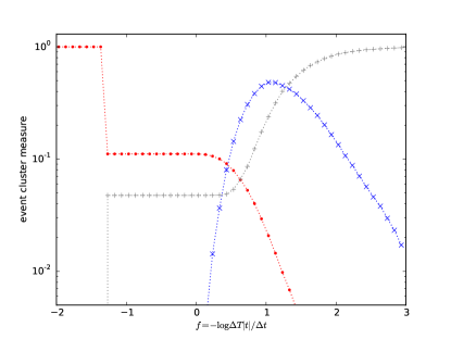
Figure 2: Sample plot of IoT service quality measures from event series $t$: $C_{t}^{o}$ ($\cdot$, red), $C_{t}^{n}$ ($\times$, blue), and $C_{t}^{s}$ ($+$, gray) by varying $\Delta T$. The series $t$ consists of a burst of random events that covers approx. 10% of the total time range $\delta t$. During the rest of the time the events are periodic at a rate of about $1/50\Delta t$.

However, our clustering output $(\tau,x)$ provides information that $n(\delta t)$ is blind to, because it does not account for the ordering of the $\delta t_{i}$. In particular,

$$C^{n}_{t}(f)=2\frac{|\tau|-\delta_{1|\tau|}}{|t|}=\begin{cases}0&\Delta T<0\\ 0\dots 1&0\leq\Delta T<\Delta t\\ 0&\Delta T\geq\Delta t\end{cases}$$ (22)

provides a normed measure of the number of clusters. While $C^{o}_{t}$ just quantifies the total coverage of $t$ by the clusters, $C_{t}^{n}$ provides insight whether the coverage is established by a number of patches or a single/a few intervals with data frequency of at least $\Delta T^{-1}$. This way we might draw conclusions on e.g. the reliability of an IoT service. Ideally we want $C^{n}_{t}\ll 1$.

Last but not least, we might consider the number of isolated events

$$C^{s}_{t}(\Delta T)=\frac{|x|}{|t|}=\begin{cases}0&\Delta T<0\\ 0\dots 1&0\leq\Delta T<\Delta t\\ 1&\Delta T\geq\Delta t\end{cases}$$ (23)

as an additional indicator of reliability, since they are orthogonal to the information contained in $\tau$. We might classify isolated events as indicator of loose IoT service quality and thus it should stay close to zero until it quickly increases to one for some $f>0$.

Figure 2 illustrates these applications by plotting $C_{t}^{o,n,s}$ for an event series $t$ generated from $10^{4}$ uniformly random samples drawn from $[0,1]$ joined by $10^{3}$ equi-distant samples in $[1,10]$. We observe that at $f=0$ there is little variance in $C_{t}^{o,s}$, indicating that there is no single dominant event frequency $\nu_{0}=|t|/\Delta t$. Moreover, there is a step in $C_{t}^{o}$ at $f\approx-1$ that covers 90% of its range which refers to a dominant event frequency one order of magnitude lower than $\nu_{0}$. Since $C_{t}^{n}\ll 1$ we conclude this frequency to be present along major time intervals within $[t_{1},t_{N}]$. Also, $C_{t}^{s}$ rapidly drops. Therefore, the existence of isolated events vanishes at time scales larger than $\sim\Delta T/10\nu_{0}$ such that we have a clean signal.

In contrast, $C_{t}^{n}\sim 1$ for $f\approx 1$. Thus, due to the randomness we introduced in our sample, for high-frequency events, increasing coverage of $[t_{1},t_{N}]$ is achieved by a number of isolated clusters (random nature of the signal!). Finally, for frequencies 3 orders of magnitude larger than $\nu_{0}$, $C_{f}^{s}\approx 1$, i.e. no more clustering of events is present.

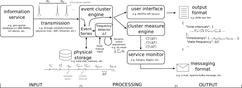
Figure 3: Sample data and processing flow of an implementation of the IoT quality service employing the procedure LABEL:lst:PseudoCodeImpl as well as the measures eqs. 20, 22 and 23. The main text provides details. Note, that here the $t_{m}$, $t_{m+1}$ and $t_{m+2}$ reference isolated timestamps of the set $x$, not to be confused with all timestamps $t_{i}$ of $t$ indexed by $i$, i.e. $x\subseteq t$.

Figure 3 depicts a sample data flow and processing pipeline where the discussed method can be employed to rate and monitor e.g. an IoT device or the data availability of satellite imagery in the big geo-spatial data platform IBM PAIRS [11, 12]. Given that this information service is expected to send data packages at frequency $\Delta T^{-1}$, an event cluster engine records and stores the timestamps $t_{i}$ for further analysis. At the same time a frequency detector might dynamically adjust $\Delta T$, e.g. by computing the mean of the $\delta t_{i}$ over a given time window. The event clustering engine is coupled to a user interface that might be interacted with by a RESTful API [13] served by e.g. Python Flask [14] to trigger the execution of LABEL:lst:PseudoCodeImpl in order to return the sets $\tau$ and $x$. Once the clustering has been performed, the quantities $C_{t}^{o,n,s}$ can be computed and analyzed by a cluster measure engine which itself feeds derived service quality indicators to a monitoring system such as e.g. Ganglia [15] or Nagios [16]. These might then release alerts by an appropriate messaging service such as plain e-mail or employing a system such as Apache Kafka [17].

III Conclusion

We discussed and implemented a one-dimensional, one-parameter clustering method with linear complexity on input and memory usage. It might be the preferred choice over the more general apporach dbscan takes when clustering ordered timestamps. Based on the algorithm’s output we suggested measures that have useful application in the domain of IoT to quantify data availability or to indicate the reliability/stability of an IoT device connecting to the network. In particular, the presented approach is part of the data availability RESTful service of IBM’s big geo-spatial database PAIRS.

The cluster method might be useful for other domains as well. Applications that have to characterize peaks of measurements can benefit. One of them is the problem of geo-locating leaks through a network of detector sensors [18] such as in the field of industrial pollution detection [19].

References

- [1] ITU-T, “Overview of the Internet of things,” 2012. [Online]. Available: http://handle.itu.int/11.1002/1000/11559
- [2] M. Chiang and T. Zhang, “Fog and IoT: An Overview of Research Opportunities,” IEEE Internet of Things Journal, vol. 3, no. 6, p. 854, 2016. [Online]. Available: http://www.download-paper.com/wp-content/uploads/2017/01/2016-ieee-Fog-and-IoT-An-Overview-of-Research-Opportunities.pdf
- [3] R. A. Fisher, “The use of multiple measurements in taxonomic problems,” Annals of eugenics, vol. 7, no. 2, p. 179, 1936. [Online]. Available: http://www.comp.tmu.ac.jp/morbier/R/Fisher-1936-Ann._Eugen.pdf
- [4] S. Lloyd, “Least squares quantization in PCM,” IEEE Transactions on Information Theory, vol. 28, no. 2, p. 129, 1982. [Online]. Available: http://www.cs.toronto.edu/~roweis/csc2515-2006/readings/lloyd57.pdf
- [5] A. P. Dempster, N. M. Laird, and D. B. Rubin, “Maximum likelihood from incomplete data via the EM algorithm,” Journal of the royal statistical society. Series B (methodological), p. 1, 1977. [Online]. Available: http://www.eng.auburn.edu/~troppel/courses/7970%202015A%20AdvMobRob%20sp15/literature/paper%20W%20refs/dempster%20EM%201977.pdf
- [6] A. Hinneburg and D. A. Keim, “An efficient approach to clustering in large multimedia databases with noise,” in KDD, vol. 98, 1998, pp. 58–65. [Online]. Available: http://www.aaai.org/Papers/KDD/1998/KDD98-009.pdf
- [7] M. Ester, H.-P. Kriegel, J. Sander, and X. Xu, “A density-based algorithm for discovering clusters in large spatial databases with noise.” in KDD, vol. 96, 1996, p. 226. [Online]. Available: http://www.aaai.org/Papers/KDD/1996/KDD96-037.pdf
- [8] I. Wegener, “The worst case complexity of McDiarmid and Reed’s variant of BOTTOM-UP HEAPSORT is less than n log n+ 1.1 n,” Information and Computation, vol. 97, no. 1, p. 86, 1992. [Online]. Available: http://www.sciencedirect.com/science/article/pii/089054019290005Z
- [9] S. v. d. Walt, S. C. Colbert, and G. Varoquaux, “The NumPy array: a structure for efficient numerical computation,” Computing in Science & Engineering, vol. 13, no. 2, pp. 22–30, 2011. [Online]. Available: https://arxiv.org/pdf/1102.1523
- [10] F. Pedregosa, G. Varoquaux, A. Gramfort, V. Michel, B. Thirion, O. Grisel, M. Blondel, P. Prettenhofer, R. Weiss, and V. Dubourg, “Scikit-learn: Machine learning in Python,” Journal of Machine Learning Research, vol. 12, no. Oct, pp. 2825–2830, 2011. [Online]. Available: http://jmlr.csail.mit.edu/papers/v12/pedregosa11a.html
- [11] L. J. Klein, F. J. Marianno, C. M. Albrecht, M. Freitag, S. Lu, N. Hinds, X. Shao, S. Bermudez Rodriguez, and H. F. Hamann, “PAIRS: A scalable geo-spatial data analytics platform,” in Big Data (Big Data), 2015 IEEE International Conference on. IEEE, 2015, pp. 1290–1298. [Online]. Available: http://researcher.watson.ibm.com/researcher/files/us-kleinl/IEEE_BigData_final_klein.pdf
- [12] S. Lu, X. Shao, M. Freitag, L. J. Klein, J. Renwick, F. J. Marianno, C. Albrecht, and H. F. Hamann, “IBM PAIRS curated big data service for accelerated geospatial data analytics and discovery,” in Big Data (Big Data), 2016 IEEE International Conference on. IEEE, 2016, pp. 2672–2675. [Online]. Available: https://static.aminer.org/pdf/fa/bigdata2016/S09208.pdf
- [13] Fielding, “Architectural Styles and the Design of Network-based Software Architectures,” Ph.D. dissertation, 2000. [Online]. Available: http://www.ics.uci.edu/~fielding/pubs/dissertation/top.htm
- [14] Wikipedia, “Flask (web framework),” 2017. [Online]. Available: https://en.wikipedia.org/wiki/Flask_(web_framework)
- [15] ——, “Ganglia (software),” 2017. [Online]. Available: https://en.wikipedia.org/wiki/Ganglia_(software)
- [16] ——, “Nagios,” 2017. [Online]. Available: https://en.wikipedia.org/wiki/Nagios
- [17] ——, “Apache Kafka,” 2017. [Online]. Available: https://en.wikipedia.org/wiki/Apache_Kafka
- [18] S. E. Haupt, “A demonstration of coupled receptor/dispersion modeling with a genetic algorithm,” Atmospheric Environment, vol. 39, no. 37, pp. 7181–7189, Dec. 2005. [Online]. Available: http://linkinghub.elsevier.com/retrieve/pii/S1352231005007685
- [19] J. D. Albertson, T. Harvey, G. Foderaro, P. Zhu, X. Zhou, S. Ferrari, M. S. Amin, M. Modrak, H. Brantley, and E. D. Thoma, “A Mobile Sensing Approach for Regional Surveillance of Fugitive Methane Emissions in Oil and Gas Production,” Environmental Science & Technology, vol. 50, no. 5, pp. 2487–2497, Mar. 2016. [Online]. Available: http://pubs.acs.org/doi/full/10.1021/acs.est.5b05059