A Simple Model for Subject Behavior
in Subjective Experiments

Abstract

In a subjective experiment to evaluate the perceptual audiovisual quality of multimedia and television services, raw opinion scores collected from test subjects are often noisy and unreliable. To produce the final mean opinion scores (MOS), recommendations such as ITU-R BT.500, ITU-T P.910 and ITU-T P.913 standardize post-test screening procedures to clean up the raw opinion scores, using techniques such as subject outlier rejection and bias removal. In this paper, we analyze the prior standardized techniques to demonstrate their weaknesses. As an alternative, we propose a simple model to account for two of the most dominant behaviors of subject inaccuracy: bias and inconsistency. We further show that this model can also effectively deal with inattentive subjects that give random scores. We propose to use maximum likelihood estimation to jointly solve the model parameters, and present two numeric solvers: the first based on the Newton-Raphson method, and the second based on an alternating projection (AP). We show that the AP solver generalizes the ITU-T P.913 post-test screening procedure by weighing a subject’s contribution to the true quality score by her consistency (thus, the quality scores estimated can be interpreted as bias-subtracted consistency-weighted MOS). We compare the proposed methods with the standardized techniques using real datasets and synthetic simulations, and demonstrate that the proposed methods are the most valuable when the test conditions are challenging (for example, crowdsourcing and cross-lab studies), offering advantages such as better model-data fit, tighter confidence intervals, better robustness against subject outliers, the absence of hard coded parameters and thresholds, and auxiliary information on test subjects. The code for this work is open-sourced at https://github.com/Netflix/sureal.

I Introduction

Subjective experiment methodologies to evaluate the perceptual audiovisual quality of multimedia and television services have been well studied. Recommendations such as ITU-R BT.500 [1], ITU-T P.910 [2] and ITU-T P.913 [3] standardize the procedures of conducting subjective experiments and post-processing raw opinion scores to produce the mean opinion scores (MOS) of test stimuli (e.g., a set of encoded videos). To account for the inherently noisy and often unreliable nature of test subjects, the recommendations have included corrective mechanisms such as subject rejection (BT.500, and also referenced in P.910 and P.913), subject bias removal (P.913), and criteria for establishing the confidence intervals of the MOS (BT.500, P.910 and P.913). The standardized procedures are not without their own limitations. For example, in BT.500, if a subject is deemed an outlier, all the raw opinion scores from that subject are discarded, which could be an overkill. The BT.500 procedure also incorporates a number of hard coded thresholds, which may not be suited for all test conditions.

As an alternative, we propose a simple model to account for two of the most dominant behaviors of test subject inaccuracy: bias and inconsistency. In addition, this model can effectively deal with inattentive subject outliers that give random scores. Compared to the BT.500-style subject rejection, the proposed model can be considered as performing “soft” subject rejection, as it explicitly models the subject outliers as having large inconsistencies, and thereby limiting their contributions to the estimated quality score through consistency weighting. To solve for the model parameters, we propose to jointly optimize the likelihood function, also known as maximum likelihood estimation (MLE) [4]. We present two numeric solvers: 1) a Newton-Raphson (NR) solver [5], and 2) an Alternating Projection (AP) solver. Compared to the NR solver which was originally developed in [6], the AP solver is faster and more intuitive. We further show that the AP solver generalizes the P.913 post-test screening procedure by weighing a subject’s contribution to the true quality score by her consistency (thus, the quality scores estimated can be thought as bias-subtractted consistency-weighted MOS). The AP solver also has the advantage of having no hard coded parameters and thresholds.

One of the challenges is to fairly compare the proposed methods to its alternatives. To this end, we evaluate the proposed simple model and its numerical solvers separately. To evaluate the model’s fit to real datasets, we use Bayesian Information Criterion (BIC) [7], where the winner can be characterized as having a good fit to data while maintaining a small number of parameters. We also compare the confidence intervals of the estimated quality scores, where a tighter confidence interval implies a higher confidence in the estimation. To evaluate the model’s robustness against subject outliers, we perform a simulation study on how the true quality score’s root mean squared error (RMSE) changes compared to the clean case as the number of outliers increases. To validate that the numerical solvers are indeed accurate, we use synthetic data to compare the recovered parameters against the ground truth. Lastly, we show that the proposed methods are the most valuable when the test conditions are challenging, by showing their advantages in a crowdsourcing test and a cross-lab study.

The rest of the paper is organized as follows. In Section II we discuss the prior art and standards. We present the proposed model in Section III, and then describe the two numerical solvers in Section IV. In Section V, we discuss two alternative ways to calculate the confidence intervals and compare their pros and cons. In Section VI we present the experimental results.

The code of this work is open-sourced on Github [8].

II Prior Art and Standards

Raw opinion scores collected from subjective experiments are known to be influenced by the inherently noisy and unreliable nature of human test subjects [9]. To compensate for the influence of individuals, a common practice is to average the raw opinion scores from multiple subjects, yielding a MOS per stimulus. Standardized recommendations incorporate more advanced corrective mechanisms to further compensate for test subjects’ influence, and criteria for establishing the confidence intervals of MOS.

• ITU-R BT.500 Recommendation [1] defines methodologies such as single-stimulus continuous quality evaluation (SSCQE), double-stimulus impairment scale (DSIS) and double-stimulus continuous quality scale (DSCQS), and a corresponding procedure for subject rejection (ITU-R BT.500-14 Section A1-2.3.1) prior to the calculation of MOS. Video by video, the procedure counts the number of instances when a subject’s opinion score deviates by a few sigmas (i.e. standard deviation), and rejects the subject if the occurrences are more than a fraction. All scores corresponding to the rejected subjects are discarded, which could be considered an overkill. On the other hand, our experiment shows that, in the presence of many outlier subjects, the procedure is only able to identify a fraction of them. In Section VI-A, we explain why this happens using a real example. Another of its drawbacks is that the incorporation of a number of hard coded parameters and thresholds to determine the outliers, which may not be suitable for all conditions. The recommendation also establishes the corresponding way of calculating the confidence interval (ITU-R BT.500-14 Section A1-2.2.1).

• ITU-T P.910 Recommendation [2] defines methodologies including absolute category rating (ACR), degradation category rating DCR (equivalent to DSIS), absolute category rating with hidden reference (ACR-HR) and the corresponding differential MOS (DMOS) calculation, and recommends using the BT.500 subject rejection and confidence interval calculation procedure in conjunction.

• ITU-T P.913 Recommendation [3] defines a procedure to remove subject bias (ITU-T P.913 Section 12.4) before carrying out other steps. It first finds the mean score per stimulus, and subtracts it from the raw opinion scores to get the residual scores. Then it averages the residue scores on a per-subject basis to yield an estimate of each subject’s bias. The biases are then removed from the raw opinion scores. For P.913 to possess resistance to subject outliers, it needs to be combined with a subject rejection strategy. P.913 recommends several ways to do so but does not mandate one (ITU-T P.913 03/2016 Section 11.4). For simplicity and consistency, in this work, we use the same one as BT.500. Yet, by doing so, it inherits similar weaknesses aforementioned.

For completeness, in Appendix A, we give mathematical descriptions of the subject rejection method standardized in ITU-R BT.500-14 and the subject bias removal method in ITU-T P.913.

III Proposed Model

We propose a simple yet effective model to account for two of the most dominant effects of test subject inaccuracy: subject bias and subject inconsistency. The model is a simplified version of [6] without considering the ambiguity of video content. Compared to the previously proposed model, the solutions to the simplified model are more efficient and stable.

Let $u_{ijr}$ be the opinion score voted by subject $i$ on stimulus $j$ in repetition $r$. We assume that each opinion score $u_{ijr}$ can be represented by a random variable as follows:

$$U_{ijr}=\psi_{j}+\Delta_{i}+\upsilon_{i}X,$$ (1)

where $\psi_{j}$ is the true quality of stimulus $j$, $\Delta_{i}$ represents the bias of subject $i$, the non-negative term $\upsilon_{i}$ represents the inconsistency of subject $i$, and $X\sim N(0,1)$ are i.i.d. Gaussian random variables. The index $r$ represents repetitions.

It is important to point out that a subject with erroneous behaviors can be modeled by a large inconsistency value $\upsilon_{i}$. The erroneous behaviors that can be modeled include but are not limited to: subject giving random scores, subject being absent-minded for a fraction of a session, or software issue that randomly shuffles a subject’s scores among multiple stimuli. By successfully estimating $\upsilon_{i}$ and accounting its effect to calculating the true quality score, we can compensate for subject outliers without invoking BT.500-style subject rejection.

Given a collection of opinion scores $\{u_{ijr}\}$ from a subjective experiment, the task is to solve for the free parameters $\theta=(\{\psi_{j}\},\{\Delta_{i}\},\{\upsilon_{i}\})$, such that the model fits the observed scores the best. This can be formulated as a maximum likelihood estimation (MLE) problem. Let the log-likelihood function be

$$L(\theta)=\log P(\{u_{ijr}\}|\{\psi_{j}\},\{\Delta_{i}\},\{\upsilon_{i}\}),$$

i.e. a monotonic measure of the probability of observing the given raw scores, for a set of these parameters. We can solve the model by finding $\hat{\theta}$ that maximizes $L(\theta)$, or $\hat{\theta}=\arg\max L(\theta)$. This problem can be numerically solved by the Newton-Raphson method or the Alternating Projection method, to be discussed in Section IV.

It is important to notice that the recoverability of $\{\psi_{j}\}$ and $\{\Delta_{i}\}$ in (1) is up to a constant shift. Formally, assume $\hat{\theta}=(\{\hat{\psi}_{j}\},\{\hat{\Delta}_{i}\},\{\hat{\upsilon}_{i}\})$ is a solution that maximizes $L(\theta)$, one can easily show that $(\{\hat{\psi}_{j}+C\},\{\hat{\Delta}_{i}-C\},\{\hat{\upsilon}_{i}\})$ where $C\in\mathbb{R}$, is another solution that achieves the same maximum likelihood value $L(\hat{\theta})$. This implies that the optimal solution is not unique. In practice, we can enforce a unique solution, by adding a constraint that forces the mean subject bias to be zero, or

$$\sum_{i}\Delta_{i}=0.$$

This intuitively makes sense, since bias is relative - saying everyone is positively biased is equivalent to saying that no one is positively biased. It is also equivalent to assuming that the sample of observers that offer opinion scores in a subjective experiment are truly random and do not consist of only “expert” viewers or “lazy” viewers that tend to offer lower or higher opinion scores, as a whole. There is always the possibility, once a subjective test establishes that the population from where subjects were recruited have such a collective bias, to change the condition and thus properly estimate what the true “typical” observer, drawn from a more representative pool that would vote.

Lastly, one should keep in mind that it is always possible to use more complicated models than (1) to capture other effects in a subjective experiment. For example, [6] considers content ambiguity, and [10, 11] considers per-stimulus ambiguity. There are also environment-related factors that could induce biases. Additionally, the votes are influenced by the voting scales chosen, for example, continuous vs. discrete [12]. Our hope is that the proposed model strikes a good balance between the model complexity and explanatory power. In Section VI-B, we show that the proposed model yields better model-data fit than the BT.500 and P.913 being used today.

IV Proposed Solvers

Let us start by simplifying the form of the log-likelihood function $L(\theta)$. We can write:

$$L(\theta) = \log P(\{u_{ijr}\}|\{\psi_{j}\},\{\Delta_{i}\},\{\upsilon_{i}\})$$

$$= \log\prod_{ijr}P(u_{ijr}|\psi_{j},\Delta_{i},\upsilon_{i})$$

$$= \sum_{ijr}\log P(u_{ijr}|\psi_{j},\Delta_{i},\upsilon_{i})$$

$$= \sum_{ijr}\log f(u_{ijr}|\psi_{j}+\Delta_{i},\upsilon_{i})$$

$$\cong \sum_{ijr}-\log\upsilon_{i}-\frac{(u_{ijr}-\psi_{j}-\Delta_{i})^{2}}{2\upsilon_{i}^{2}}$$ (3)

where (IV) uses the independence assumption on opinion scores, $f(x|\mu,\upsilon)$ denotes the Gaussian density function with mean $\mu$ and standard deviation $\upsilon$, and $\cong$ denotes omission of constant terms.

Note that not every subject needs to vote on each stimulus in every repetition. Our proposed solvers can effectively deal with subjective tests with incomplete data where some observations $u_{ijr}$ are missing. Denote by $\star$ the missing observations in an experiment. All summations in this paper are ignoring the missing observations $\star$, that is, $\sum_{ijr}$ is equivalent to $\sum_{ijr:u_{ijr}\neq\star}$, and so on.

IV-A Newton-Raphson (NR) Solver

With (3), the first- and second-order partial derivatives of $L(\theta)$ can be derived (see Section B). We can apply the Newton-Raphson rule [5] $a^{new}\leftarrow a-\frac{\partial L/\partial a}{\partial^{2}L/\partial a^{2}}$ to update each parameter $a$ in iterations. We further use a refresh rate parameter $\alpha$ to control the innovation rate to avoid overshooting. Note that other update rules can be applied, but using the Newton-Raphson rule yields nice interpretability.

Also note that the NR solver finds a local optimal solution when the problem is non-convex. It is important to initialize the parameters properly. We choose zeros as the initial values for $\{\Delta_{i}\}$, the mean score $MOS_{j}=(\sum_{ir}1)^{-1}\sum_{ir}u_{ijr}$ for $\{\psi_{j}\}$, and the residue standard deviation $RSD_{i}=\sigma_{i}(\{\epsilon_{ijr}\})$ for $\{\upsilon_{i}\}$, where $\epsilon_{ijr}=u_{ijr}-MOS_{j}$ is the “residue”, $\sigma_{i}(\{\epsilon_{ijr}\})=\sqrt{(\sum_{jr}1)^{-1}\sum_{jr}(\epsilon_{ijr}-\epsilon_{i})^{2}}$, and $\epsilon_{i}=(\sum_{jr}1)^{-1}\sum_{jr}\epsilon_{ijr}$. The NR solver is summarized in Algorithm 1. A good choice of innovation rate and stop threshold are $\alpha=0.1$ and $\psi^{thr}=1e^{-9}$, respectively, but varying these parameters would not significantly change the result.

• Input:

  • $u_{ijr}$ for subject $i=1,...,I$, stimulus $j=1,...,J$ and repetition $r=1,...,R$.

  • Refresh rate $\alpha$.

  • Stop threshold $\psi^{thr}$.

• Initialize $\{\Delta_{i}\}\leftarrow\{0\}$, $\{\psi_{j}\}\leftarrow\{MOS_{j}\}$, $\{\upsilon_{i}\}\leftarrow\{RSD_{i}\}$.

• Loop:

  • $\{\psi_{j}^{prev}\}\leftarrow\{\psi_{j}\}$.

  • $\Delta_{i}\leftarrow(1-\alpha)\cdot\Delta_{i}+\alpha\cdot\Delta_{i}^{new}$ where $\Delta_{i}^{new}=\Delta_{i}-\frac{\partial L(\theta)/\partial\Delta_{i}}{\partial^{2}L(\theta)/\partial\Delta_{i}^{2}}$ for $i=1,...,I$.

  • $\upsilon_{i}\leftarrow(1-\alpha)\cdot\upsilon_{i}+\alpha\cdot\upsilon_{i}^{new}$ where $\upsilon_{i}^{new}=\upsilon_{i}-\frac{\partial L(\theta)/\partial\upsilon_{i}}{\partial^{2}L(\theta)/\partial\upsilon_{i}^{2}}$ for $i=1,...,I$.

  • $\psi_{j}\leftarrow(1-\alpha)\cdot\psi_{j}+\alpha\cdot\psi_{j}^{new}$ where $\psi_{j}^{new}=\psi_{j}-\frac{\partial L(\theta)/\partial\psi_{j}}{\partial^{2}L(\theta)/\partial\psi_{j}^{2}}$ for $j=1,...,J$.

  • If $\left(\sum_{j=1}^{J}(\psi_{j}-\psi_{j}^{prev})^{2}\right)^{\frac{1}{2}}<\psi^{thr}$, break.

• Output: $\{\psi_{j}\}$, $\{\Delta_{i}\}$, $\{\upsilon_{i}\}$.

Algorithm 1 Proposed Newton-Raphson (NR) solver

The “new” parameters can be simplified to the following form:

$$\psi_{j}^{new} = \frac{\sum_{ir}\upsilon_{i}^{-2}(u_{ijr}-\Delta_{i})}{\sum_{ir}\upsilon_{i}^{-2}},$$ (4)

$$\Delta_{i}^{new} = \frac{\sum_{jr}(u_{ijr}-\psi_{j})}{\sum_{jr}1},$$ (5)

$$\upsilon_{i}^{new} = \upsilon_{i}\frac{\sum_{jr}2\upsilon_{i}^{2}-4(u_{ijr}-\psi_{j}-\Delta_{i})^{2}}{\sum_{jr}\upsilon_{i}^{2}-3(u_{ijr}-\psi_{j}-\Delta_{i})^{2}}.$$

Note that there are strong intuitions behind the expressions for the newly estimated true quality $\psi_{j}^{new}$ and subject bias $\Delta_{i}^{new}$. In each iteration, $\psi_{j}^{new}$ is re-estimated, as the weighted mean of the opinion scores $u_{ijr}$ with the currently estimated subject bias $\Delta_{i}$ removed. Each opinion score is weighted by the “subject consistency” $\upsilon_{i}^{-2}$, i.e., the higher the inconsistency for subject $i$, the less reliable the opinion score, hence less the weight. For the subject bias $\Delta_{i}^{new}$, it is simply the average shift between subject $i$’s opinion scores and the true values.

IV-B Alternating Projection (AP) Solver

This solver is called “alternating projection” because in a loop, it alternates between projecting (or averaging) the opinion scores along the subject dimension and the stimulus dimension. To start, we initialize $\{\psi_{j}\}$ to $\{MOS_{j}\}$, where $MOS_{j}=(\sum_{ir}1)^{-1}\sum_{ir}u_{ijr}$, same as the NR solver. The subject bias $\{\Delta_{i}\}$ is initialized differently to $\{BIAS_{i}\}$, where $BIAS_{i}=(\sum_{jr}1)^{-1}\sum_{jr}(u_{ijr}-MOS_{j})$ is the average shift between subject $i$’s opinion scores and the true values. Note that the calculation of $\{MOS_{j}\}$ and $\{BIAS_{i}\}$ matches precisely to the ones in Algorithm 4 (ITU-T P.913). Within the loop, first, the “residue” $\epsilon_{ijr}$ is updated, followed by the calculation of the subject inconsistency $\upsilon_{i}$ as the residue’s standard deviation per subject $\sigma_{i}(\{\epsilon_{ijr}\})$, with:

$$\sigma_{i}(\{\epsilon_{ijr}\}) = \sqrt{(\sum_{jr}1)^{-1}\sum_{jr}(\epsilon_{ijr}-\epsilon_{i})^{2}},$$ (6)

$$\epsilon_{i} = (\sum_{jr}1)^{-1}\sum_{jr}\epsilon_{ijr}.$$ (7)

Then, the true quality $\{\psi_{j}\}$ and the subject bias $\{\Delta_{i}\}$ are re-estimated, by averaging the opinion scores along either the subject dimension $i$ or the stimulus dimension $j$. The projection formula precisely matches equations (4) and (5) of the Newton-Raphson method. The AP solver is summarized in Algorithm 2. A good choice of the stop threshold is $\psi^{thr}=1e^{-8}$.

The AP solver generalizes the P.913 post-test screening (Section 12.4) in the following sense. First, the AP solver is iterative until convergence whereas P.913 only goes through the initialization steps. Second, in the AP solver, the re-estimation of quality score $\psi_{j}$ is weighted by the subject consistency $\upsilon_{i}^{-2}$ whereas in P.913, the re-estimation is unweighted. Please note that weighting multiple random variables by the inverse of their variance is the minimum error parameter estimation, as can be trivially proven through Lagrange multipliers. Intuitively, the estimated quality scores of the AP solver can be regarded as bias-subtracted consistency-weighted MOS.

• Input:

  • $u_{ijr}$ for subject $i=1,...,I$, stimulus $j=1,...,J$ and repetition $r=1,...,R$.

  • Stop threshold $\psi^{thr}$.

• Initialize $\{\psi_{j}\}\leftarrow\{MOS_{j}\}$, $\{\Delta_{i}\}\leftarrow\{BIAS_{i}\}$.

• Loop:

  • $\{\psi_{j}^{prev}\}\leftarrow\{\psi_{j}\}$.

  • $\epsilon_{ijr}=u_{ijr}-\psi_{j}-\Delta_{i}$ for $i=1,...,I$, $j=1,...,J$ and $r=1,...,R$.

  • $\upsilon_{i}\leftarrow\sigma_{i}(\{\epsilon_{ijr}\})$ for $i=1,...,I$.

  • $\psi_{j}\leftarrow\frac{\sum_{ir}\upsilon_{i}^{-2}(u_{ijr}-\Delta_{i})}{\sum_{ir}\upsilon_{i}^{-2}}$ for $j=1,...,J$.

  • $\Delta_{i}\leftarrow\frac{\sum_{jr}(u_{ijr}-\psi_{j})}{\sum_{jr}1},$ for $i=1,...,I$.

  • If $\left(\sum_{j=1}^{J}(\psi_{j}-\psi_{j}^{prev})^{2}\right)^{\frac{1}{2}}<\psi^{thr}$, break.

• Output: $\{\psi_{j}\}$, $\{\Delta_{i}\}$, $\{\upsilon_{i}\}$.

Algorithm 2 Proposed Alternating Projection (AP) solver

V Confidence Interval

The estimation of each model parameter $\{\psi_{j}\}$, $\{\Delta_{i}\}$, $\{\upsilon_{i}\}$ is associated with a confidence interval (CI). One way to calculate the CIs is through their asymptotic analytical forms. Using the Cramer-Rao bound [13], the asymptotic $95\%$ confidence intervals for the mean terms $\psi_{j}$ and $\Delta_{i}$ have the form $CI(a)=a\pm 1.96\left(-\frac{\partial^{2}L(a)}{\partial a^{2}}\right)^{-\frac{1}{2}}$, where their second-order derivatives $\frac{\partial^{2}L(a)}{\partial a^{2}}$ can be found in Section B. The $95\%$ confidence interval for the standard deviation term $\upsilon_{i}$ has the form $\left(\sqrt{\frac{k}{\chi_{k}^{2}(0.975)}}\upsilon,\sqrt{\frac{k}{\chi_{k}^{2}(0.025)}}\upsilon\right)$, where $\chi_{k}^{2}(a)$ is the percent point function (i.e. the inverse of the cumulative distribution function) of a chi-square distribution with $k$ degrees of freedom. After simplification, the confidence intervals for $\psi_{j}$, $\Delta_{i}$ and $\upsilon_{i}$ are:

$$CI(\psi_{j}) = \psi_{j}\pm 1.96\frac{1}{\sqrt{\sum_{ir}\upsilon_{i}^{-2}}},$$ (8)

$$CI(\Delta_{i}) = \Delta_{i}\pm 1.96\frac{\upsilon_{i}}{\sqrt{\sum_{jr}1}},$$

$$CI(\upsilon_{i}) = \left(\begin{array}[]{cc}\sqrt{\frac{k_{i}}{\chi_{k_{i}}^{2}(0.975)}}\upsilon_{i},&\sqrt{\frac{k_{i}}{\chi_{k_{i}}^{2}(0.025)}}\upsilon_{i}\end{array}\right),$$ (10)

where $k_{i}=\sum_{jr}1$ is the number of samples that subject $i$ has viewed.

There is one practical limitation with Equation (8). Recall that $\sum_{ir}$ is equivalent to $\sum_{ir:u_{ijr}\neq\star}$, where $\star$ represents missing observation. If there is no missing observations (i.e. every subject votes on every stimulus), then the lengths of the confidence intervals for $\psi_{j}$, $j=1,...,J$ will be all equal to the same value $\frac{3.92}{\sqrt{\sum_{ir}\upsilon_{i}^{-2}}}$ (since it is independent of the subscript $j$). In other words, we have equal confidence in the estimation of quality scores $\psi_{j}$, $j=1,...,J$. Although this is theoretically correct (since all quality scores are estimated jointly) and it results in the tightest CIs, it deviates from a conventional approach (for example, plain MOS, or BT.500), where each quality score has a different CI length (see Section C for a MLE interpretation of the plain MOS). Practically, it raises the concern that the CIs are unable to capture the behaviors of individual stimuli.

To address this concern, we propose an alternative calculation of CI for $\psi_{j}$, which yields looser but discriminative CIs. Let $\upsilon_{j}=\sigma_{j}(\{\epsilon_{ijr}\})$ denote the per-stimulus variability, where $\sigma_{j}(\{\epsilon_{ijr}\})$ is the per-stimulus standard deviation of the residues $\{\epsilon_{ijr}\}$, with:

$$\sigma_{j}(\{\epsilon_{ijr}\}) = \sqrt{(\sum_{ir}1)^{-1}\sum_{ir}(\epsilon_{ijr}-\epsilon_{j})^{2}},$$ (11)

$$\epsilon_{j} = (\sum_{ir}1)^{-1}\sum_{ir}\epsilon_{ijr}.$$ (12)

The alternative CI for $\psi_{j}$ (denoted by $CI_{2}$) can then be calculated as:

$$CI_{2}(\psi_{j})=\psi_{j}\pm 1.96\frac{\upsilon_{j}}{\sqrt{\sum_{ir}1}}.$$ (13)

Comparing (11) (12) with (6) (7), one can see that the main difference is the “projection direction” in the tensor $\{\epsilon_{ijr}\}$ when calculating the mean and the standard deviation. Through simulations, we will show in Section VI-E that $CI_{2}$ is also theoretically correct, although it yields less tight CIs. In the following sections, the AP solver combined with $CI_{2}$ is denoted by AP2.

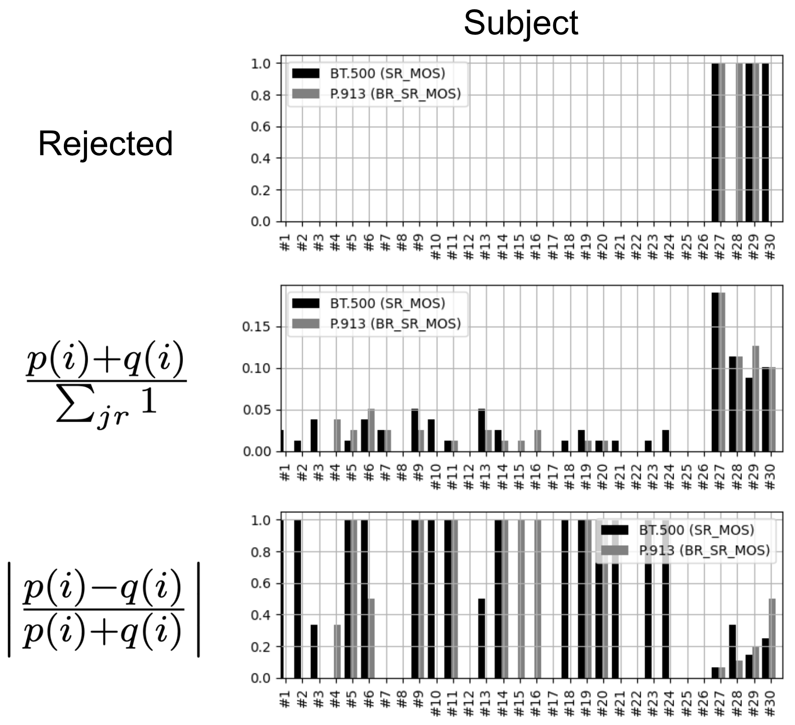
Figure 1: Subject rejection result by BT.500 and P.913 on the NFLX Public dataset. The top plot shows the final rejection result, where value 1.0 means rejected and 0.0 means not rejected. The middle and bottom plots show the intermediate result of $(\sum_{jr}1)^{-1}(p(i)+q(i))$ and $\left|(p(i)+q(i))^{-1}(p(i)-q(i))\right|$, respectively. (SR: subject rejection; BR: bias removal.)

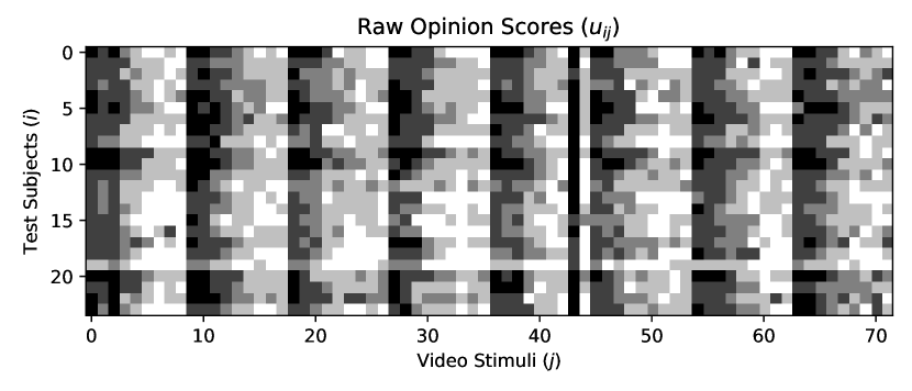
(a) VQEG HD3 dataset

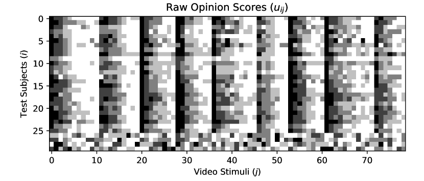
(b) NFLX Public dataset

Figure 2: Raw opinion scores from (a) the VQEG HD3 dataset [14] and (b) the NFLX Public dataset [15]. Each pixel represents a raw opinion score. The darker the color, the lower the score. The impaired videos are arranged by contents, and within each content, from low quality to high quality (with the reference video always appears last). For the NFLX Public dataset, the last four rows correspond to corrupted subjective data.

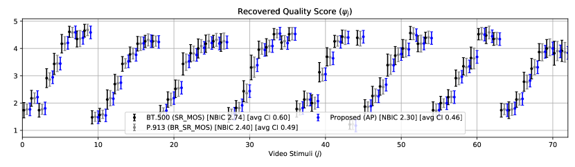
(a) VQEG HD3 dataset

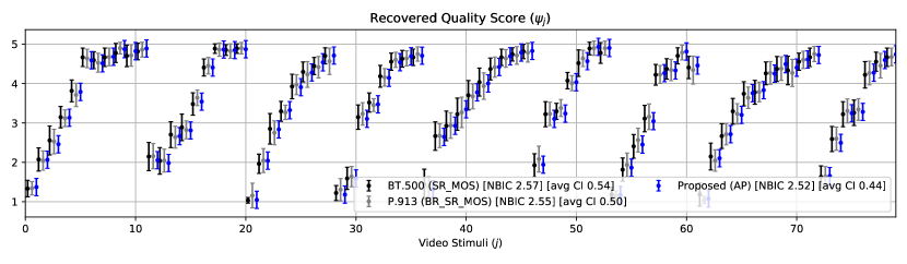
(b) NFLX Public dataset

Figure 3: Recovered quality score $\psi_{j}$ and its confidence interval (based on (8)) for the four methods compared, on (a) the VQEG HD3 dataset and (b) the NFLX Public dataset. The proposed NR method is not shown in the plots since it virtually produces identical results as the proposed AP method. For each method compared, the NBIC score (see Section VI-B) and the average length of the confidence interval are reported. (SR: subject rejection; BR: bias removal; avg CI: average confidence interval; NBIC: Bayesian Information Criterion; NR: Newton-Raphson; AP: Alternating Projection.)

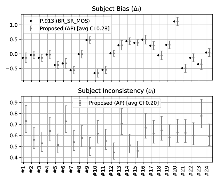
(a) VQEG HD3 dataset

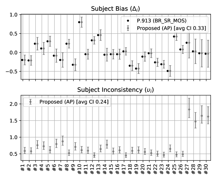
(b) NFLX Public dataset

Figure 4: Recovered subject bias $\Delta_{i}$ and subject inconsistency $\upsilon_{i}$ for each subject $i$, for the methods compared, on (a) the VQEG HD3 dataset and (b) the NFLX Public dataset. The proposed NR method is not shown in the plots since it virtually produces identical results as the proposed AP method. For each method compared, the average length of the confidence interval is reported. (SR: subject rejection; BR: bias removal; avg CI: average confidence interval; NR: Newton-Raphson; AP: Alternating Projection.)

VI Experimental Results

We compare the proposed method (the proposed model and its two numerical solvers) with the prior art BT.500 and P.913 recommendations. We first illustrate the proposed model by giving visual examples on two datasets: VQEG HD3 dataset [14] (which is the compression-only subset of the larger HDTV Ph1 Exp3 dataset) and the NFLX Public dataset [15]. We then validate the model-data fit using the Bayesian Information Criterion (BIC) on 22 datasets, including 20 datasets as part of a different larger experiments: VQEG HDTV Phase I [14]; ITS4S [16]; AGH/NTIA [10, 17]; MM2 [18]; ITU-T Supp23 Exp1 [19]; and ITS4S2 [20]. We also evaluate the confidence intervals on the estimated quality scores on these 22 datasets. Next, we demonstrate that the proposed model is much more effective in dealing with outlier subjects. Lastly, we use synthetic data to validate the accuracy of the numerical solvers and the confidence interval calculation. Lastly, we show that the proposed method is most valuable when the test conditions are challenging, by showing their advantages in a crowdsourcing test conducted at Netflix and the VQEG FRTV Phase I cross-lab study [21].

VI-A Visual Examples

First, we demonstrate the proposed method on the VQEG HD3 and the NFLX Public datasets. Refer to Figure 2 for a visualization of the raw opinion scores. The 44th video of the VQEG HD3 dataset has a quality issue such that all its scores are low. The NFLX Public dataset includes four subjects whose raw scores were shuffled due to a software issue during data collection.

Figure 3 shows the recovered quality scores of the four methods compared. The quality scores recovered by the two proposed methods are numerically different from the ones of BT.500 and P.913, suggesting that the recovery is non-trivial. The average confidence intervals (based on (8)) by the proposed methods are generally tighter, compared to the ones of BT.500 and P.913, suggesting that the estimation has higher confidence. Due to clutteredness, we do not plot the alternative $CI_{2}$ (13) in Figure 3, but will show them in Section VI-C. The NBIC scores, to be discussed in detail in Section VI-B, represent how well the model fits the data. It can be observed that the proposed model fits the data better than BT.500 and P.913.

Figure 4 shows the recovered subject bias and subject inconsistency by the methods compared. On the VQEG HD3 dataset, it can be seen that the 20th subject has the most positive bias, which is evidenced by the whitish horizontal strip visible in Figure 2 (a). On the NFLX Public dataset, the last four subjects, whose raw scores are scrambled, have very high subject inconsistency values. Correspondingly, their estimated biases have very loose confidence intervals. This illustrates that the proposed model is effective in modeling outlier subjects.

The subject bias and inconsistency revealed through the recovery process could be valuable information for subject screening. Unlike BT.500, which makes a binary decision on if a subject is accepted/rejected, the proposed approach characterizes a subject’s inaccuracy in two dimensions, along with their confidence intervals, allowing further interpretation and study. How to use the bias and inconsistency information to better screen subjects remains our future work.

VI-A1 Comparison with BT.500 and P.913

As a comparison, we also visualize the subject rejection results from BT.500 and P.913 on the NFLX Public dataset, as shown in Figure 1. These recommendations encode the hard rule that if

$$\frac{p(i)+q(i)}{\sum_{jr}1}\geq 0.05$$ (14)

and

$$\left|\frac{p(i)-q(i)}{p(i)+q(i)}\right|<0.3,$$ (15)

subject $i$ is rejected. Intuitively, (14) looks at the fraction of scores that are considered outliers. As shown in the middle plot of Figure 1, for both BT.500 and P.913, all four outliers meet this criterion. The real problem lies in (15), which says that subject $i$ is rejected only if the distribution is not too skewed. The rule itself seems benign, as it tests the skewness of the distribution and only when the distribution is not too skewed, (14) should apply. But by this rule, for either BT.500 and P.913, only three out of four outliers meet the hard-coded threshold of 0.3. This example exposes the limitation of the hard-coded rules in BT.500 and P.913. On the contrary, the proposed method does not use hard-coded rules, thus is immune from this problem.

VI-B Model-Data Fit

Bayesian Information Criterion (BIC) [7] is a criterion for model-data fit. When fitting models, it is possible to increase the likelihood by adding parameters, but doing so may result in overfitting. BIC attempts to balance between the degree of freedom (characterized by the number of free parameters) and the goodness of fit (characterized by the log-likelihood function). Formally, BIC is defined as $BIC=\log(n)|\theta|-2L(\theta)$, where $n=|\{u_{ijr}\}|$ is the total number of observations (i.e. the number of opinion scores), $|\theta|$ is the number of model parameters, and $L(\theta)$ is the log-likelihood function. One can interpret that the lower the free parameter numbers $|\theta|$, and the higher the log-likelihood $L(\theta)$, the lower the BIC, and hence the better fit. In this work, we adopt the notion of a normalized BIC (NBIC), defined as the BIC divided by the number of observations, or:

$$NBIC=\frac{\log(n)|\theta|-2L(\theta)}{n},$$

as the model fit criterion, for easier comparison across datasets (since different datasets have a different $n$).

Table I shows the NBIC reported on the compared methods on the 22 public datasets. The MOS method is the plain MOS without subject rejection or subject bias removal. $|\theta|$ for MOS and BT.500 is $2J$, where $J$ is the number of stimuli (refer to Section C for a MLE interpretation of the plain MOS). For P.913, $|\theta|$ is equal to $2J+I$, where $I$ is the number of subjects (due to the subject bias term). For the calculation of the log-likelihood function, notice that if subject rejection is applied, only the opinion scores after rejection are taken into account. The result in Table I shows that the proposed two solvers yield better model-data fit than the plain MOS, BT.500 and P.913 approaches.

Dataset	MOS	BT.500	P.913	NR/AP
VQEG HD3	2.75	2.74	2.39	2.30
NFLX Public	2.97	2.57	2.55	2.52
HDTV Ph1 Exp1	2.45	2.46	2.38	2.20
HDTV Ph1 Exp2	2.72	2.72	2.52	2.32
HDTV Ph1 Exp3	2.72	2.71	2.37	2.29
HDTV Ph1 Exp4	2.96	2.96	2.51	2.27
HDTV Ph1 Exp5	2.77	2.77	2.47	2.33
HDTV Ph1 Exp6	2.51	2.49	2.32	2.16
ITU-T Supp23 Exp1	2.91	2.91	2.35	2.31
MM2 1	2.80	2.78	2.83	2.74
MM2 2	3.89	3.89	3.52	3.13
MM2 3	2.48	2.47	2.45	2.41
MM2 4	2.74	2.73	2.62	2.47
MM2 5	2.90	2.82	2.67	2.64
MM2 6	2.81	2.74	2.74	2.72
MM2 7	2.73	2.72	2.76	2.67
MM2 8	3.00	2.92	2.88	2.70
MM2 9	3.27	3.21	2.95	2.79
MM2 10	3.04	3.05	2.98	2.82
its4s2	3.63	3.63	2.96	2.59
its4s AGH	3.15	3.05	2.77	2.64
its4s NTIA	2.94	2.91	2.53	2.38

TABLE I: NBIC reported on the compared methods on public datasets. The NR and AP (and AP2) methods produce identical results. (MOS: plain mean opinion score; NR: Newton-Raphson; AP: Alternating Projection.)

VI-C Confidence Interval of Quality Scores

Table II shows the average length of the CIs on the compared methods on the 22 public datasets. The smaller the number, the tighter the CI, thus more confident the estimation is. For MOS, BT.500 and P.913, the CIs are calculated based on (17). For BT.500 and P.913, only the opinions scores after rejection are taken into account. For the proposed methods NR and AP, the CIs are calculated based on (8). The proposed alternative $CI_{2}$ (13) combined with AP is denoted by AP2. It can be observed that the NR and AP yield the tightest CIs compared to the other methods. AP2 also yields very tight CIs, except for the NFLX public dataset, where the four outliers’ very loose CIs contributed to the loosening of the overall CIs (0.57). For some databases, BT.500 generates wider confidence interval than the plain MOS. This can be explained by the fact that subject rejection decreases the number of samples, even though the variance may also be decreased. Overall, the obtained confidence interval can be either narrower or wider.

To visually compare the CIs for AP and AP2, we plot them in Figure 5. It can be observed that AP yields constant CIs across the stimuli whereas AP2 yields differentiated CIs.

Dataset	MOS	BT.500	P.913	NR/AP (AP2)
VQEG HD3	0.59	0.60	0.49	0.46 (0.47)
NFLX Public	0.62	0.54	0.5	0.44 (0.57)
HDTV Ph1 Exp1	0.50	0.61	0.48	0.46 (0.46)
HDTV Ph1 Exp2	0.57	0.57	0.53	0.48 (0.49)
HDTV Ph1 Exp3	0.56	0.59	0.52	0.48 (0.48)
HDTV Ph1 Exp4	0.63	0.63	0.52	0.47 (0.49)
HDTV Ph1 Exp5	0.57	0.57	0.53	0.49 (0.50)
HDTV Ph1 Exp6	0.50	0.51	0.48	0.45 (0.45)
ITU-T Supp23 Exp1	0.61	0.61	0.56	0.47 (0.50)
MM2 1	0.59	0.60	0.57	0.53 (0.55)
MM2 2	1.21	1.21	1.12	0.88 (0.99)
MM2 3	0.47	0.48	0.45	0.42 (0.43)
MM2 4	0.58	0.59	0.54	0.48 (0.51)
MM2 5	0.63	0.65	0.58	0.52 (0.56)
MM2 6	0.62	0.70	0.59	0.56 (0.57)
MM2 7	0.60	0.61	0.57	0.55 (0.55)
MM2 8	0.76	0.76	0.71	0.66 (0.68)
MM2 9	0.84	0.85	0.74	0.68 (0.71)
MM2 10	0.77	0.83	0.73	0.70 (0.70)
its4s2	0.82	0.82	0.66	0.60 (0.64)
its4s AGH	0.68	0.68	0.61	0.56 (0.60)
its4s NTIA	0.57	0.58	0.54	0.48 (0.50)

TABLE II: Average length of confidence intervals of the estimated quality scores reported on the compared methods on public datasets. The NR and AP methods are based on (8) and they produce identical results. AP2 is the AP method combined with the alternative CI calculation (13). MOS: arithmetic mean of all opinion scores; NR: Newton-Raphson; AP: Alternating Projection.

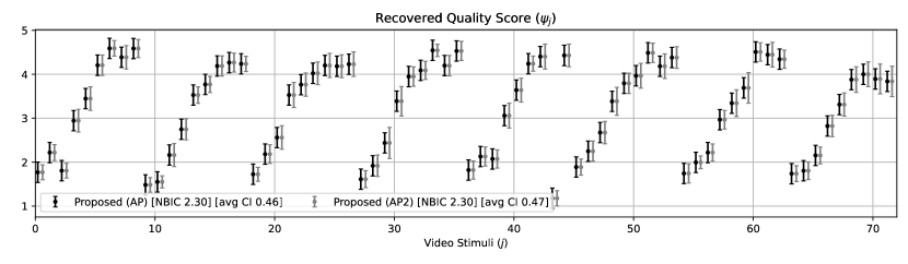
(a) VQEG HD3 dataset

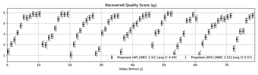
(b) NFLX Public dataset

Figure 5: Recovered quality score $\psi_{j}$ and its CI for AP (CI based on (8)) and AP2 (CI based on (13)) on (a) the VQEG HD3 dataset and (b) the NFLX Public dataset. For each method compared, the NBIC score (see Section VI-B) and the average length of the confidence interval are reported. (avg CI: average confidence interval; NBIC: Bayesian Information Criterion; AP: Alternating Projection.)

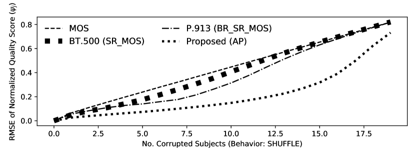
(a) VQEG HD3 dataset

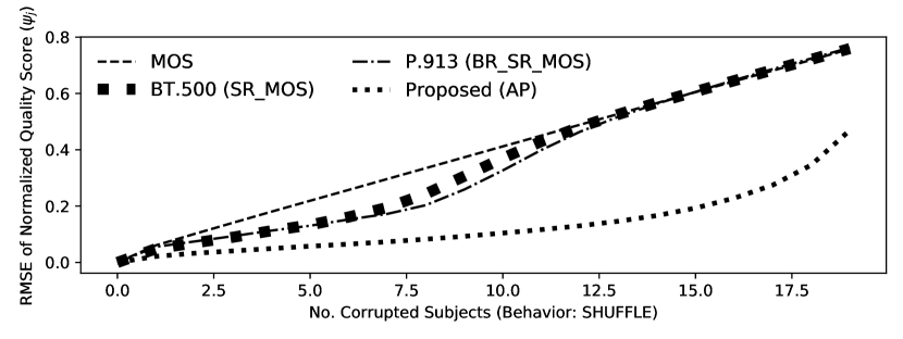
(b) NFLX Public dataset

Figure 6: RMSE of the (normalized) recovered quality score $\psi_{j}$ as a function of the number of corrupted subjects, of the proposed method (AP) versus the other methods, of (a) the VQEG HD3 dataset and (b) the NFLX Public dataset. The NR and AP solvers yield identical results. The subject corruption is simulated, in the way that the scores corresponding to a subject are scrambled. The recovered quality score is normalized by subtracting the mean and dividing by the standard deviation of the scores of the unaltered dataset. (MOS: plain mean opinion score; SR: Subject Rejection; BR: Bias Removal; AP: Alternating Projection.)

(a) VQEG HD3 dataset

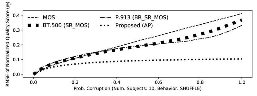
(b) NFLX Public dataset

Figure 7: RMSE of the (normalized) recovered quality score $\psi_{j}$ as a function of the probability of corruption (fixing the number of corrupted subjects to 10), of the proposed method (AP) versus the other methods, of (a) the VQEG HD3 dataset and (b) the NFLX Public dataset. The NR and AP solvers yield identical results. The subject corruption is simulated, in the way that the scores corresponding to a subject are scrambled. The recovered quality score is normalized by subtracting the mean and dividing by the standard deviation of the scores of the unaltered dataset. (MOS: plain mean opinion score; SR: Subject Rejection; BR: Bias Removal; AP: Alternating Projection.)

VI-D Robustness against Outlier Subjects

We demonstrate that the proposed method is much more effective in dealing with (corrupted) outlier subjects compared to other methods. We use the following methodology in our reporting of results. For each method compared, we have a benchmark result, which is the recovered quality scores obtained using that method - for fairness - on an unaltered full dataset (note that for the NFLX Public dataset, unlike the one used in Figure 2, 3 and 4, we start with the dataset where the corruption on the last four subjects has been corrected). We then consider that a number of the subjects are “corrupted” and simulate it by randomly shuffling each corrupted subject’s votes among the video stimuli. We then run each method compared on the partially corrupted datasets. The quality scores recovered are normalized by subtracting the mean and dividing by the standard deviation of the scores of the unaltered dataset. The normalized scores are compared against the benchmark, and a root-mean-squared-error (RMSE) value is reported.

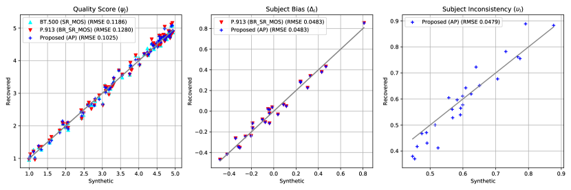
(a) Comparing BT.500, P.913 and AP

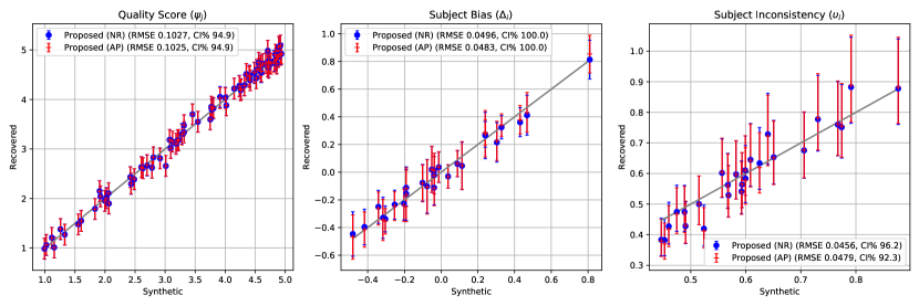
(b) Confidence Intervals of NR and AP

Figure 8: Validation of the proposed NR and AP solvers using synthetic data. The random samples are generated using the following methodology. For each proposed solver, take the NFLX Public dataset, run the solver to estimate the parameters. Treat the estimated parameters as the “synthetic” parameters (or the ground truth), run simulations to generate synthetic samples according to the model (1). Run the solver again on the synthetic data to yield the “recovered” parameters. The x-axis shows the synthetic parameters and the y-axis shows the recovered parameters. (a) Comparing the proposed AP with BT.500 and P.913, (b) Proposed NR and AP with confidence intervals. (NR: Newton-Raphson; AP: Alternating Projection.)

Figure 6 reports the results on the two datasets, comparing the proposed method with plain MOS, BT.500, P.913 and the proposed NR and AP solvers, as the number of corrupted subjects increases. It can be observed that in the presence of subject corruption, The proposed method achieves a substantial gain over the other methods. The reason is that the proposed model was able to capture the variance of subjects explicitly and is able to compensate for it. On the other hand, the other methods are only able to identify part of the corrupted subjects. Meanwhile, traditional subject rejection employs a set of hard coded parameters to determine outliers, which may not be suited for all conditions. By contrast, the proposed model naturally integrates the various subjective effects together and is solved efficiently by the MLE formulation. In particular, the AP solver can be interpreted as averaging the scores weighted by subject’s consistency. For corrupted subjects with large inconsistency scores, their contribution to the final quality scores are limited.

Figure 7 reports the results as we increase the probability of corruption from 0 to 1 while fixing the number of corrupted subjects to 10. It can be seen that as the corruption probability increases, the RMSE increases linearly/near-linearly for other methods, while the RMSE increases much slower for the proposed method, and it saturates at a constant value without increasing further. A simplified explanation is that, since only a subset of a subject’s scores is unreliable, discarding all of the subject’s scores is a waste of valuable subjective data, while the proposed methods can effectively avoid that.

VI-E Validations Using Synthetic Data

Next, we demonstrate that the NR and AP solvers can accurately recover the parameters of the proposed model. This is shown using synthetic data, where the ground truth of the model parameters are known. In this section, we considered only the NFLX Public dataset for simulations. The random samples are generated using the following methodology. For each proposed solver, we take the NFLX Public dataset and run the solver to estimate the parameters. The parameters estimated from a real dataset allow us to run simulations with practical settings. We then treat the estimated parameters as the “synthetic” parameters (hence the ground truth), run simulations to generate synthetic samples according to the model (1). Subsequently, we run the solver again on the synthetic data to yield the “recovered” parameters.

VI-E1 Validation of Solvers

Figure 8 shows the scatter plots of the synthetic vs. recovered parameters, for the true quality $\psi_{j}$, subjective bias $\Delta_{i}$ and subject inconsistency $\upsilon_{i}$ terms. It can be observed that the solvers recover the parameters reasonably well. We have to keep in mind that the synthetic data, differently from usual subjective scores of category rating, are continuous. For discrete data, some specific problems would influence the obtained results as described in [12]. Since those problems are not the main topic of this paper we do not go into more details and leave it as a future topic of research.

Figure 8(a) also shows the recovery result of the BT.500 and P.913. It is noticeable that the recovered subject biases by the AP method and the P.913 subject bias removal are very similar. This should not be surprising, considering that the AP method can be treated as a weighted and iterative generalization of the P.913 method.

Dataset	MOS	NR			AP (AP2)
	$\psi_{j}$	$\psi_{j}$	$\Delta_{i}$	$\upsilon_{i}$	$\psi_{j}$	$\Delta_{i}$	$\upsilon_{i}$
VQEG HD3	93.3	93.6	93.9	93.0	93.2 (93.5)	94.4	91.9
NFLX Public	94.2	93.7	94.5	93.1	93.5 (97.5)	94.1	92.3
HDTV Ph1 Exp1	93.9	94.1	93.9	93.1	93.8 (93.2)	94.2	91.3
HDTV Ph1 Exp2	93.8	94.0	94.5	92.5	93.8 (94.1)	94.0	91.2
HDTV Ph1 Exp3	93.9	93.9	94.4	92.5	93.7 (93.6)	94.1	90.6
HDTV Ph1 Exp4	93.8	94.0	94.3	91.9	93.8 (94.1)	94.1	90.9
HDTV Ph1 Exp5	93.8	94.1	94.2	92.2	93.9 (93.8)	94.2	90.9
HDTV Ph1 Exp6	93.8	94.0	94.4	92.6	93.9 (93.6)	94.0	91.0
ITU-T Supp23 Exp1	93.8	94.0	94.4	91.2	93.8 (94.5)	94.9	90.0
MM2 1	93.5	92.8	95.4	92.6	92.5 (93.8)	94.0	91.6
MM2 2	92.1	81.5	92.9	80.0	68.1 (87.5)	92.1	75.4
MM2 3	94.4	93.6	95.1	93.4	93.4 (94.1)	94.2	92.0
MM2 4	93.2	93.6	95.6	93.0	93.2 (94.7)	95.1	92.0
MM2 5	93.2	93.2	95.7	92.7	91.8 (94.3)	95.3	91.4
MM2 6	93.6	93.3	95.2	92.8	93.0 (93.8)	94.1	91.4
MM2 7	93.6	93.3	95.2	92.8	92.9 (93.2)	94.2	91.9
MM2 8	93.0	92.4	95.4	88.8	92.2 (92.6)	94.5	87.0
MM2 9	93.2	93.3	94.8	89.1	92.8 (93.3)	94.2	88.1
MM2 10	93.2	93.1	95.7	89.7	92.8 (92.3)	94.5	87.9
its4s2	93.1	94.1	94.6	60.6	94.1 (94.0)	94.2	59.2
its4s AGH	93.6	94.0	94.4	90.4	94.0 (94.8)	94.4	89.7
its4s NTIA	93.9	94.4	94.7	86.1	94.3 (95.0)	95.1	85.6

TABLE III: Average confidence interval coverage (CI%) reported on public datasets. For each proposed solver and each dataset, run the solver to estimate the parameters. Treat the estimated parameters as “synthetic” parameters, run simulations to generate synthetic samples according to the model (1) (except for MOS, whose samples are generated according to (16)). Run the solver again on the synthetic data to yield the “recovered” parameters and their confidence intervals. The reported “CI%” is the percentage of occurrences when the synthetic ground truth falls within the confidence interval. For each dataset, the simulation is run 100 times with different seeds. Note that for both MOS and the proposed NR and AP methods, the CI% is slightly below 95%, due to the underlying Gaussian assumption used instead of the legitimate Student’s t-distribution. (MOS: plain mean opinion score; NR: Newton-Raphson; AP: Alternating Projection.) For $\psi_{j}$ of AP, two CI% are reported: the CI based on (8) and (in the parenthesis) the alternative CI calculated based on (13).

Dataset	Mean Runtime (seconds)					No. Iterations
	MOS	BT.500	P.913	NR	AP	NR	AP
VQEG HD3	5.2e-4	1.5e-2	1.5e-2	2.1e-1	4.3e-3	26.2	12.1
NFLX Public	5.7e-4	1.8e-2	1.9e-2	2.8e-1	4.5e-3	34.5	11.8
HDTV Ph1 Exp1	7.7e-4	3.3e-2	3.4e-2	2.0e-1	4.6e-3	23.4	10.3
HDTV Ph1 Exp2	7.8e-4	3.3e-2	3.4e-2	2.8e-1	4.9e-3	33.2	11.3
HDTV Ph1 Exp3	7.8e-4	3.3e-2	3.4e-2	2.5e-1	4.7e-3	29.4	10.7
HDTV Ph1 Exp4	7.6e-4	3.3e-2	3.4e-2	3.3e-1	5.0e-3	38.3	11.5
HDTV Ph1 Exp5	7.8e-4	3.3e-2	3.4e-2	2.7e-1	4.7e-3	31.3	10.8
HDTV Ph1 Exp6	7.6e-4	3.3e-2	3.4e-2	2.2e-1	4.6e-3	25.8	10.7
ITU-T Supp23 Exp1	8.1e-4	3.5e-2	3.5e-2	3.4e-1	5.0e-3	36.0	11.6
MM2 1	4.9e-4	1.3e-2	1.3e-2	2.1e-1	4.3e-3	27.4	12.4
MM2 2	4.0e-4	1.0e-2	1.1e-2	5.8e-1	1.4e-2	78.0	54.9
MM2 3	5.3e-4	1.3e-2	1.4e-2	1.8e-1	4.2e-3	23.3	11.6
MM2 4	5.0e-4	1.3e-2	1.4e-2	2.6e-1	4.6e-3	33.4	13.8
MM2 5	5.0e-4	1.3e-2	1.4e-2	2.9e-1	6.0e-3	37.3	19.3
MM2 6	4.8e-4	1.2e-2	1.3e-2	2.2e-1	4.3e-3	28.8	13.1
MM2 7	4.8e-4	1.2e-2	1.3e-2	2.0e-1	4.2e-3	25.6	12.3
MM2 8	4.3e-4	1.1e-2	1.1e-2	2.7e-1	5.5e-3	35.3	18.7
MM2 9	4.3e-4	1.1e-2	1.2e-2	2.8e-1	5.1e-3	36.5	16.8
MM2 10	4.3e-4	1.1e-2	1.2e-2	2.3e-1	4.8e-3	29.8	15.4
its4s2	3.3e-3	2.5e-1	2.5e-1	1.1e+0	1.3e-2	49.8	13.3
its4s AGH	8.7e-4	4.1e-2	4.2e-2	3.5e-1	5.3e-3	39.4	11.6
its4s NTIA	2.6e-3	1.6e-1	1.6e-1	6.4e-1	1.1e-2	46.2	11.3

TABLE IV: Average runtime in seconds and number of iterations (for NR and AP) reported on public datasets. AP2 has the same runtime as AP. For each proposed solver and each dataset, run the solver to estimate the parameters. Treat the estimated parameters and the “synthetic” parameters, run simulations to generate synthetic samples according to the model (1) (except for MOS, whose samples are generated according to (16)). Run the solver again on the synthetic data. For each dataset, the simulation is run 100 times with different seeds, and the mean is reported. For NR and AP, also reported are the number of iterations. (MOS: plain mean opinion score; NR: Newton-Raphson; AP: Alternating Projection.)

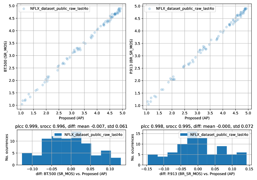
(a) NFLX Public dataset (lab test)

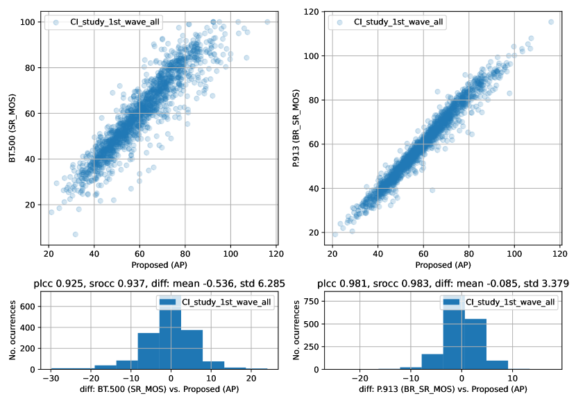
(b) NFLX Crowdsourcing 1st Wave dataset

Figure 9: Scatter plots of recovered quality scores $\psi_{j}$ between BT.500 and AP (left) and between P.913 and AP (right) for (a) the NFLX Public dataset and (b) NFLX Crowdsourcing 1st Wave dataset. The diagram below shows the histogram of the difference values. The Pearson correlation (PLCC), Spearman correlation (SROCC), the mean and the standard deviation of the difference values are also reported. The NR and AP solvers yield identical results. (MOS: plain mean opinion score; SR: Subject Rejection; BR: Bias Removal; AP: Alternating Projection.)

VI-E2 Validation of Confidence Intervals

Also plotted in Figure 8(b) are the confidence intervals of the recovered parameters. The reported “CI%” is the percentage of occurrences where the synthetic ground truth falls within the confidence interval. By definition, we expect the CI% to be 95% on average. To verify this, we run the same simulation on the 22 public datasets. For each dataset, the simulation is run 100 times with different seeds. The result is shown in Table III. We compare the proposed NR and AP methods with the plain MOS. It can be seen that all methods yield CI% to be very close to 95%, but slightly below. The explanation is that both have assumed that the underlying distribution is Gaussian, but with both the mean and standard deviation unknown, one should use a Student’s t-distribution instead. If the t-distribution is used, the coefficient can no longer be a fixed value 1.96 but is a function of the number of subjects and repetitions.

VI-F Runtime and Iterations

We then evaluate the runtime of the proposed NR and AP methods compared to the others. The results of 100 simulations runs (based on the similar methodology as in the previous sections) of each methods are reported in Table IV. The results reveal the order of magnitude of the algorithms compared. The plain MOS is typically the fastest, while the BT.500 and P.913 are two magnitude slower. The NR and AP algorithms are three and one magnitude slower, respectively. Noteably, the AP runs faster than BT.500 and P.913, and is about 50x faster than the NR. The AP also requires about half the number of iterations to reach convergence than the NR.

VI-G Consistency Under Challenging Conditions

In this section, we demonstrate that the proposed methods are the most valuable when the test conditions are challenging. Traditional lab tests are typically conducted in a highly controlled environment. When analyzing the different methods using these lab datasets, we find that the recovered quality scores using BT.500, P.913 and the proposed AP (and NR) method are highly consistent. However, when the test conditions are challenging, for example, in a crowdsourced test, the different methods could yield quite inconsistent results. This is illustrated in Figure 9, where the quality scores recovered by different methods are compared in scatter plots. Figure 9 (a) is based on the NFLX Public dataset (a lab test), and Figure 9 (b) is based on a crowdsourced test conducted by Netflix (details to follow). It can be seen that the results from the crowdsourced test are much less consistent across methods.

Which method yields the most accurate recovery? Unfortunately, we cannot directly answer this question since we do not have the ground truth. However, we can demonstrate that the proposed AP method can yield more consistency (or less variability), and thus is more desirable. We demonstrate this using 1) the crowdsourced test where we correlate the result using all the data with the one using only 10% of the data, and 2) a cross-lab test, where the same stimuli are tested at different lab locations.

VI-G1 NFLX Crowdsourcing Test

The NFLX Crowdsourcing Test was conducted on 154 video contents and 1859 video stimuli, each 10-second long. It consists of two datasets: 1) the 1st Wave dataset, a small pre-test with 20 votes per stimulus on average, and 2) the 2nd Wave dataset, the full test with 290 votes per stimulus on average. In this section, we use the 2nd Wave dataset. For each of the methods evaluated, we compare the quality scores recovered using the full dataset with the scores recovered using only 10% of the data, randomly sampled. The scatter plots are shown in Figure 10, which also reports the correlations and the mean and standard deviation of the difference values. It can be seen that the proposed AP method yields the best consistency and the least variability among the three methods. In addition, P.913 does better than BT.500, due to the removal of the subject bias.

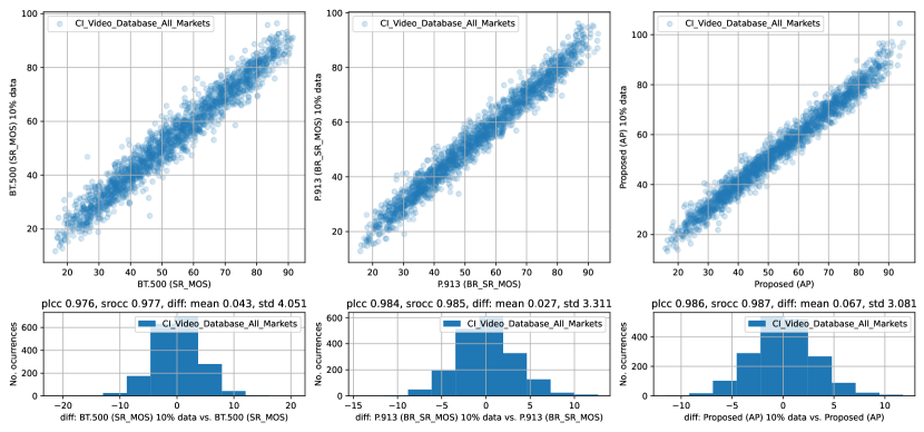
Figure 10: Scatter plots of recovered quality scores $\psi_{j}$ between using full data (x-axis) vs. using only 10% of the data (randomly sampled, y-axis) of the NFLX Crowdsourcing 2nd Wave dataset. The left, middle and right plots are based on BT.500, P.913 and the proposed AP, respectively. The diagram below shows the histogram of the difference values. The Pearson correlation (PLCC), Spearman correlation (SROCC), the mean and the standard deviation of the difference values are also reported. The NR and AP solvers yield identical results. (MOS: plain mean opinion score; SR: Subject Rejection; BR: Bias Removal; AP: Alternating Projection.)

Lab	1	4	6	8
1	1.0	0.944	0.943	0.948
4		1.0	0.957	0.941
6			1.0	0.944
8				1.0

BT.500

Lab	1	4	6	8
1	1.0	0.950	0.942	0.95
4		1.0	0.9556	0.940
6			1.0	0.944
8				1.0

P.913

Lab	1	4	6	8
1	1.0	0.952	0.949	0.958
4		1.0	0.957	0.945
6			1.0	0.948
8				1.0

Proposed AP

(a) 525 Line Low

Lab	1	4	6	8
1	1.0	0.890	0.900	0.915
4		1.0	0.881	0.850
6			1.0	0.875
8				1.0

BT.500

Lab	1	4	6	8
1	1.0	0.888	0.903	0.906
4		1.0	0.867	0.834
6			1.0	0.874
8				1.0

P.913

Lab	1	4	6	8
1	1.0	0.906	0.911	0.915
4		1.0	0.876	0.823
6			1.0	0.833
8				1.0

Proposed AP

(b) 525 Line High

Lab	2	3	5	7
2	1.0	0.743	0.913	0.914
3		1.0	0.812	0.705
5			1.0	0.900
7				1.0

BT.500

Lab	2	3	5	7
2	1.0	0.764	0.908	0.904
3		1.0	0.840	0.755
5			1.0	0.905
7				1.0

P.913

Lab	2	3	5	7
2	1.0	0.814	0.926	0.923
3		1.0	0.875	0.804
5			1.0	0.918
7				1.0

Proposed AP

(c) 625 Line Low

Lab	2	3	5	7
2	1.0	0.790	0.853	0.818
3		1.0	0.818	0.836
5			1.0	0.869
7				1.0

BT.500

Lab	2	3	5	7
2	1.0	0.764	0.794	0.737
3		1.0	0.826	0.834
5			1.0	0.849
7				1.0

P.913

Lab	2	3	5	7
2	1.0	0.829	0.818	0.800
3		1.0	0.825	0.860
5			1.0	0.874
7				1.0

Proposed AP

(d) 625 Line High

TABLE V: Cross-lab Pearson correlation coefficient (PLCC) results for the VQEG FRTV Phase I study. The study produces four datasets: 1) 525 Line Low, 2) 525 Line High, 3) 625 Line Low and 4) 625 Line High. In total 8 labs participated in the study, and each dataset is evaluated by 4 of the 8 labs. The quality scores are recovered by three methods: BT.500, P.913 and the proposed AP. The best result among the three methods is in bold.

VI-G2 VQEG FRTV Phase I Study

The VQEG full-reference television (FRTV) Phase I study [21] examines full-reference objective quality models that predicted the quality of standard definition television (625-line and 525-line). The study produces four datasets: 1) 525 Line Low, 2) 525 Line High, 3) 625 Line Low and 4) 625 Line High. In total 8 labs participated in the study, and each dataset is evaluated by 4 of the 8 labs. Table V shows the cross-lab Pearson correlation coefficient. The quality scores are recovered by three methods: BT.500, P.913 and the proposed AP. From the result, one can conclude that among the three methods, statistically, the proposed AP method yields the best consistency across labs.

VII Conclusions

In the paper, we proposed a simple model to account for two of the most dominant effects of test subject inaccuracy: subject bias and subject inconsistency. We further proposed to solve the model parameters through maximum likelihood estimation and presented two numerical solvers. We compared the proposed methodology with the standardized recommendations including ITU-R BT.500 and ITU-T P.913, and showed that the proposed methods are the most valuable when the test conditions are challenging (for example, crowdsourcing and cross-lab studies), offering advantages such as better model-data fit, tighter confidence intervals, better robustness against subject outliers, the absence of hard coded parameters and thresholds, and auxiliary information on test subjects. We believe the proposed methodology is generally suitable for subjective evaluation of perceptual audiovisual quality in multimedia and television services, and we propose to update the corresponding recommendations with the methods presented.

Appendix A Mathematical Descriptions of BT.500 and P.913

A-A BT.500 Subject Rejection

In this section, we give mathematical descriptions of the subject rejection method standardized in ITU-R BT.500-14 and the subject bias removal method in ITU-T P.913. Let $u_{ijr}$ be the opinion score voted by subject $i$ on stimulus $j$ in repetition $r$. Note that, in BT.500-14, the notation $j$ is used to indicate test condition and $k$ is used to indicate sequence/image; in this paper, the test condition and sequence/image are combined and collectively represented by the stimulus notation $j$. Let $\mu_{jr}$ denote the mean value over scores for stimulus $j$ and for repetition $r$, i.e. $\mu_{jr}=(\sum_{i}1)^{-1}\sum_{i}u_{ijr}$ . Similarly, $m_{n,jr}$ denotes the $n$-th order central moment over scores for stimulus $j$ and repetition $r$, i.e. $m_{n,jr}=(\sum_{i}1)^{-1}\sum_{i}(u_{ijr}-\mu_{jr})^{n}$. Lastly, $\sigma_{jr}$ denotes the sample standard deviation for stimulus $j$ and repetition $r$, i.e. $\sigma_{jr}=\sqrt{\left((\sum_{i}1)-1\right)^{-1}\sum_{i}(u_{ijr}-\mu_{jr})^{2}}$. In the previous, the term $\sum_{i}1$ indicates the number of observers that have offered an opinion score for a given stimulus/repetition, $jr$. This number of observers could be the same, $I$, or different per stimulus, if a subjective experiment has been designed in such a way. The subject rejection procedure in ITU-R BT.500-14 Section A1-2.3 can be summarized in Algorithm 3.

A-B P.913 Subject Bias Removal

ITU-T P.913 does not consider repetitions, so the notation $u_{ij}$ denotes the opinion score voted by subject $i$ on stimulus $j$. The subject bias removal procedure in ITU-T P.913 Section 12.4 can be summarized in Algorithm 4.

After subject bias removal, we assume that the subject rejection described in Algorithm 3 is carried out, before calculating the MOS and the corresponding confidence intervals. Note that P.913 recommends several subject rejection strategies but does not mandate one (ITU-T P.913 (03/2016) Section 11.4). For simplicity and consistency, we use the same one as BT.500.

Appendix B Appendix: First- and Second-Order Partial Derivatives of $L(\theta)$

We can derive the first-order and second-order partial derivatives of $L(\theta)$ with respect to $\psi_{j}$ , $\Delta_{i}$ and $\upsilon_{i}$ as:

$$\frac{\partial L(\theta)}{\partial\psi_{j}} = \sum_{ir}\frac{u_{ijr}-\psi_{j}-\Delta_{i}}{\upsilon_{i}^{2}}$$

$$\frac{\partial L(\theta)}{\partial\Delta_{i}} = \sum_{jr}\frac{u_{ijr}-\psi_{j}-\Delta_{i}}{\upsilon_{i}^{2}}$$

$$\frac{\partial L(\theta)}{\partial\upsilon_{i}} = \sum_{jr}-\frac{1}{\upsilon_{i}}+\frac{(u_{ijr}-\psi_{j}-\Delta_{i})^{2}}{\upsilon_{i}^{3}}$$

$$\frac{\partial^{2}L(\theta)}{\partial\psi_{j}^{2}} = -\sum_{ir}\frac{1}{\upsilon_{i}^{2}}$$

$$\frac{\partial^{2}L(\theta)}{\partial\Delta_{i}^{2}} = -\frac{1}{\upsilon_{i}^{2}}\sum_{jr}1$$

$$\frac{\partial^{2}L(\theta)}{\partial\upsilon_{i}^{2}} = \sum_{jr}\frac{1}{\upsilon_{i}^{2}}-\frac{3(u_{ijr}-\psi_{j}-\Delta_{i})^{2}}{\upsilon_{i}^{4}}$$

Appendix C An MLE Interpretation of the Plain MOS

The plain MOS and its confidence interval can be interpreted using the notion of maximum likelihood estimation. Consider the model:

$$U_{ijr}=\psi_{j}+\upsilon_{j}X,$$ (16)

where $U_{ijr}$ is the opinion score, $\psi_{j}$ is the true quality of stimulus $j$ and $\upsilon_{j}$ is the “ambiguity” of $j$. $X\sim N(0,1)$ is i.i.d. Gaussian. Note that this is different from the proposed model (1) where $\upsilon_{i}$ is associated with the subjects, not the stimuli. We can define the log-likelihood function for this model as $L(\theta)=\log P(\{u_{ijr}\}|(\{\psi_{j}\},\{\upsilon_{j}\}))$, and solve for $\{\psi_{j}\}$ and $\{\upsilon_{j}\}$ that maximize the log-likelihood function, as follows:

$$\psi_{j} = \frac{\sum_{ir}u_{ijr}}{\sum_{ir}1},$$

$$\upsilon_{j} = \sqrt{\frac{\sum_{ir}(u_{ijr}-\psi_{j})^{2}}{\sum_{ir}1}.}$$

The second-order partial derivative w.r.t. to $\psi_{j}$ is $\frac{\partial^{2}L(\theta)}{\partial\psi_{j}^{2}}=-\frac{1}{\upsilon_{j}^{2}}\sum_{ir}1$. The 95% confidence interval of $\psi_{j}$ is then:

$$CI(\psi_{j})=\psi_{j}\pm 1.96\frac{\upsilon_{j}}{\sqrt{\sum_{ir}1}}.$$ (17)

One minor difference between (17) and the 95% confidence interval formula in BT.500-14 Section A1-2.2.1 is that the former uses differential degrees of freedom 0 and the latter uses 1 for the sample standard deviation calculation. In fact, neither one is fully precise. In the most precise way to calculate the confidence interval, one should use a Student’s t-distrubiton with a differential degrees of freedom 1 (see Section VI-E and Table III for more discussions).

• Input: $u_{ijr}$ for $i=1,...,I$, $j=1,...,J$ and $r=1,...,R$.

• Initialize $p(i)\leftarrow 0$ and $q(i)\leftarrow 0$ for $i=1,...,I$.

• For $j=1,...,J$, $r=1,...,R$:

  • Let $Kurtosis_{jr}=\frac{m_{4,jr}}{\left(m_{2,jr}\right)^{2}}$.

  • If $2\leq Kurtosis_{jr}\leq 4$, then $\epsilon_{jr}=2$; otherwise $\epsilon_{jr}=\sqrt{20}$.

  • For $i=1,...,I$:

    • If $u_{ijr}\geq\mu_{jr}+\epsilon_{jr}\sigma_{jr}$, then $p(i)\leftarrow p(i)+1.$

    • If $u_{ijr}\leq\mu_{jr}-\epsilon_{jr}\sigma_{jr}$, then $q(i)\leftarrow q(i)+1$.

• Initialize $Set_{rej}=\emptyset$.

• For $i=1,...,I$:

  • If $\frac{p(i)+q(i)}{\sum_{jr}1}\geq 0.05$ and $\left|\frac{p(i)-q(i)}{p(i)+q(i)}\right|<0.3$, then $Set_{rej}\leftarrow Set_{rej}\cup\{i\}.$

• Output: $Set_{rej}$.

Algorithm 3 ITU-R BT.500 Subject Rejection [1]

• Input:

  • $u_{ij}$ for subject $i=1,...,I$, stimulus $j=1,...,J$.

• For $j=1,...,J$:

  • Estimate MOS of stimulus as $MOS_{j}=(\sum_{i}1)^{-1}\sum_{i}u_{ij}$.

• For $i=1,...,I$:

  • Estimate subject bias as $BIAS_{i}=(\sum_{j}1)^{-1}\sum_{j}(u_{ij}-MOS_{j})$.

• Calculate the subject bias-removed opinion scores $r_{ij}=u_{ij}-BIAS_{i}$, $i=1,...,I$, $j=1,...,J$.

• Use $r_{ij}$ instead of $u_{ij}$ as the opinion scores to carry out the remaining steps.

Algorithm 4 ITU-T P.913 Subject Bias Removal [3]

References

- [1] ITU-R BT.500-14 (10/2019): Methodologies for the Subjective Assessment of the Quality of Television Images. https://www.itu.int/rec/R-REC-BT.500.
- [2] ITU-T P.910 (04/08): Subjective Video Quality Assessment Methods for Multimedia Applications. https://www.itu.int/rec/T-REC-P.910.
- [3] ITU-T P.913 (03/2016): Methods for the Subjective Assessment of Video Quality, Audio Quality and Audiovisual Quality of Internet Video and Distribution Quality Television in Any Environment. https://www.itu.int/rec/T-REC-P.913.
- [4] Maximum Likelihood Estimation (Wikipedia). https://en.wikipedia.org/wiki/Maximum_likelihood_estimation. [Online; accessed 30-March-2020].
- [5] Newton’s Method in Optimization (Wikipedia). https://en.wikipedia.org/wiki/Newton%27s_method_in_optimization. [Online; accessed 30-March-2020].
- [6] Zhi Li and Christos G. Bampis. Recover Subjective Quality Scores from Noisy Measurements. https://arxiv.org/abs/1611.01715. in Proceedings of the Data Compression Conference, 2017.
- [7] Bayesian Information Criterion (Wikipedia). https://en.wikipedia.org/wiki/Bayesian_information_criterion. [Online; accessed 30-March-2020].
- [8] SUREAL - Subjective Recovery Analysis. https://github.com/Netflix/sureal. [Online; accessed 30-March-2020].
- [9] Tobias Hoßfeld, Raimund Schatz, and Sebastian Egger. SOS: The MOS is not enough! 2011 3rd International Workshop on Quality of Multimedia Experience, QoMEX 2011, pages 131–136, 2011.
- [10] L. Janowski and M. Pinson. Subject bias: Introducing a theoretical user model. In 2014 Sixth International Workshop on Quality of Multimedia Experience (QoMEX), pages 251–256, Sep. 2014.
- [11] L. Janowski and M. Pinson. The accuracy of subjects in a quality experiment: A theoretical subject model. IEEE Transactions on Multimedia, 17(12):2210–2224, Dec 2015.
- [12] Lucjan Janowski, Bogdan Ćmiel, Krzysztof Rusek, Jakub Nawała, and Zhi Li. Generalized score distribution. https://arxiv.org/abs/1909.04369. in arXiv:1909.04369 [stat.ME], 2019.
- [13] T.M. Cover and J.A. Thomas. Elements of Information Theory. A Wiley-Interscience publication. Wiley, 2006.
- [14] Margaret Pinson, Filippo Speranza, M Barkowski, V Baroncini, R Bitto, S Borer, Y Dhondt, R Green, L Janowski, T Kawano, et al. Report on the validation of video quality models for high definition video content. Video Quality Experts Group, 2010.
- [15] Netflix Public Dataset. https://github.com/Netflix/vmaf/blob/master/resource/doc/datasets.md. [Online; accessed 30-March-2020].
- [16] Margaret H. Pinson. Its4s: A video quality dataset with four-second unrepeated scenes. Technical Report NTIA Technical Memo TM-18-532, NTIA/ITS, Feb. 2018.
- [17] Margaret H. Pinson and L. Janowski. Agh/ntia: A video quality subjective test with repeated sequences. Technical Report NTIA Technical Memo TM-14-505, NTIA/ITS, June 2014.
- [18] M. H. Pinson, L. Janowski, R. Pepion, Q. Huynh-Thu, C. Schmidmer, P. Corriveau, A. Younkin, P. Le Callet, M. Barkowsky, and W. Ingram. The influence of subjects and environment on audiovisual subjective tests: An international study. IEEE Journal of Selected Topics in Signal Processing, 6(6):640–651, Oct 2012.
- [19] ITU-T P-Series. ITU-T coded-speech database. Technical Report Series P: Telephone Transmission Quality, Telephone Installations, Local Line Networks, ITU-T, Feb. 1998.
- [20] Margaret H. Pinson. ITS4S2: An image quality dataset with unrepeated images from consumer cameras,. Technical Report NTIA Technical Memo TM-19-537, NTIA/ITS, Apr. 2019.
- [21] VQEG FRTV (Full Reference Television) Phase I Project Page. https://www.its.bldrdoc.gov/vqeg/projects/frtv-phase-i/frtv-phase-i.aspx. [Online; accessed 17-April-2021].