Presupernova neutrinos: directional sensitivity and prospects for progenitor identification

Abstract

We explore the potential of current and future liquid scintillator neutrino detectors of $\mathcal{O}(10)$ kt mass to localize a pre-supernova neutrino signal in the sky. In the hours preceding the core collapse of a nearby star (at distance $D\lesssim 1$ kpc), tens to hundreds of inverse beta decay events will be recorded, and their reconstructed topology in the detector can be used to estimate the direction to the star. Although the directionality of inverse beta decay is weak ($\sim$ 8% forward-backward asymmetry for currently available liquid scintillators), we find that for a fiducial signal of $200$ events (which is realistic for Betelgeuse), a positional error of $\sim$ 60^∘ can be achieved, resulting in the possibility to narrow the list of potential stellar candidates to less than ten, typically. For a configuration with improved forward-backward asymmetry ($\sim$ 40%, as expected for a lithium-loaded liquid scintillator), the angular sensitivity improves to $\sim$ 15^∘, and – when a distance upper limit is obtained from the overall event rate – it is in principle possible to uniquely identify the progenitor star. Any localization information accompanying an early supernova alert will be useful to multi-messenger observations and to particle physics tests using collapsing stars.

1 Introduction

Over the next decade, neutrino astronomy will probe the rich astrophysics of neutrino production in the sky. In addition to neutrinos from the Sun (Borexino Collaboration et al., 2018), core-collapse supernova bursts (e.g., SN 1987A, Hirata et al., 1987, 1988; Bionta et al., 1987; Alekseev et al., 1987), and relativistic jets (e.g., blazar TXS 0506+056, IceCube Collaboration et al., 2018a, b), technological improvements in detector masses, energy resolution and background abatement will allow to observe new signals from different stages of the lifecycle of stars, in particular presupernova neutrinos (Odrzywolek et al., 2004a), the diffuse supernova neutrino background (Bisnovatyi-Kogan & Seidov, 1984; Krauss et al., 1984), and neutrinos from matter-rich binary mergers (Kyutoku & Kashiyama, 2018; Lin & Lunardini, 2020). Ultimately, the goal will be to test neutrino production across the entire Hertzsprung-Russell diagram (Farag et al., 2020).

Presupernova neutrinos are the neutrinos of $\sim$ 0.1 - 5 MeV energy that accompany, with increasing luminosity, the last stages of nuclear burning of a massive star in the days leading to its core collapse and final explosion as a supernova, or implosion into a black hole (a “failed” supernova). These neutrinos are produced by thermal processes – mainly pair-production – that depend on the ambient thermodynamic conditions (Fowler & Hoyle, 1964; Beaudet et al., 1967; Schinder et al., 1987; Itoh et al., 1996) – and by weak reactions – mainly electron/positron captures and nuclear decays – that have a stronger dependence on the isotopic composition (Fuller et al., 1980, 1982a, 1982b, 1985; Langanke & Martínez-Pinedo, 2000, 2014; Misch et al., 2018), and thus on the network of nuclear reactions that take place in the stellar interior.

Building on early calculations (Odrzywolek et al., 2004a, b; Kutschera et al., 2009; Odrzywolek, 2009), recent numerical simulations with state-of-the-art treatment of the nuclear processes (Kato et al., 2015; Yoshida et al., 2016; Patton et al., 2017a, b; Kato et al., 2017; Guo et al., 2019) have shown that the presupernova neutrino flux increases dramatically, both in luminosity and in average energy, in the hours prior to the collapse, and it becomes potentially detectable when silicon burning is ignited in the core of the star. In particular, for stars within $\sim$ 1 kpc of Earth like Betelgeuse, presupernova neutrinos will be detected at multi-kiloton neutrino detectors like the current KamLAND (see Araki et al. (2005) for a dedicated study), Borexino (Borexino Collaboration et al., 2018), SNO+ (Andringa et al., 2016), Daya Bay (Guo et al., 2007) and SuperKamiokande (Simpson et al., 2019), and the upcoming HyperKamiokande (Abe et al., 2016), DUNE (Acciarri et al., 2016) and JUNO (An et al., 2016; Li, 2014; Brugière, 2017). Next generation dark matter detectors like XENON (Newstead et al., 2019), DARWIN (Aalbers et al., 2016), and ARGO (Aalseth et al., 2018) will also observe a significant signal (Raj et al., 2020). Therefore, presupernova neutrinos are a prime target for the SuperNova Early Warning System network (SNEWS, Antonioli et al., 2004) – which does or will include the neutrino experiments mentioned above – and its multi-messenger era successor SNEWS 2.0, whose mission is to provide early alerts to the astronomy and gravitational wave communities, and to the scientific community at large as well. The observation of presupernova neutrinos from an impending core-collapse supernova will: (i) allow numerous tests of stellar and neutrino physics, including tests of exotic physics that may require pointing to the collapsing star (e.g. axion searches, see Raffelt et al. (2011)); and (ii) enable a very early alert of the collapse and supernova, thus extending – perhaps crucially, especially for envelope-free stellar progenitors that tend to explode shortly after collapse – the time frame available to coordinate multi-messenger observations.

In this paper, we explore presupernova neutrinos as early alerts. In particular, we focus on the question of localization: can a signal of presupernova neutrinos provide useful positional information? Can it identify the progenitor star? From a recent exploratory study (Li et al., 2020), we know that the best potential for localization is offered by inverse beta decay events at large (${\mathcal{O}}(10)$ kt mass) liquid scintillator detectors, where, for optimistic presupernova flux predictions and a star like Betelgeuse (distance of 0.2 kpc), a signal can be discovered days before the collapse, and the direction to the progenitor can be determined with a $\sim 80^{\circ}$ error.

This article is the first dedicated study on the localization question for presupernova neutrinos. Using a state-of-the-art numerical model for the neutrino emission, we examine a number of questions that were not previously discussed, having to do with the diverse stellar population of nearby stars (including red and blue supergiants, of masses between $\sim$ 10 and $\sim$ 30 times the mass of the Sun, and clustered in certain regions of the sky) and with the rich possibilities of improving the directionality of the liquid scintillator technology in the future.

In Section 2 we discuss presupernova neutrino event rates and nearby candidates. In Section 3 we present our main results for the angular sensitivity. In Section 4 we discuss progenitor identification, and in Section 5 we summarize our results. In Appendix A we detail the distance and mass estimates of nearby presupernova candidates.

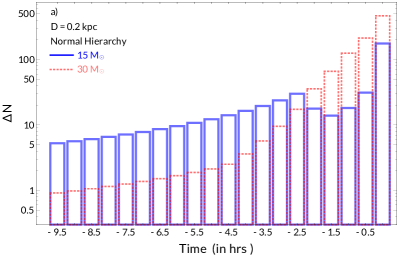
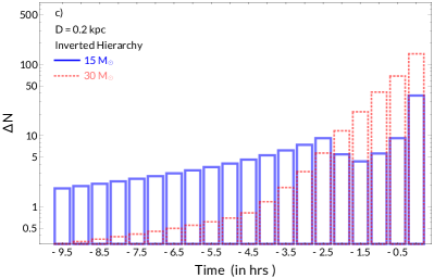
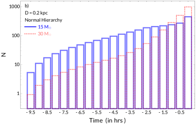
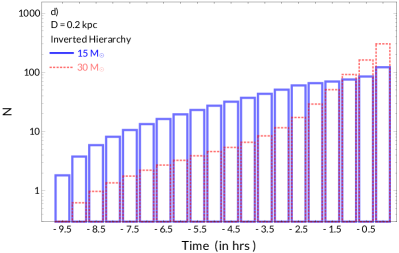
Figure 1: Top row a) and c): Number of presupernova neutrino events at a 17 kt liquid scintillator detector, in time bins of width $\Delta t=0.5$ hrs as a function of time before core-collapse. Bottom row or b) and d): Cumulative numbers of events in half-hour increments. Shown are the cases of a ZAMS 15 $\mathrel{{M_{\odot}}}$ (blue histogram) and a ZAMS 30 $\mathrel{{M_{\odot}}}$ (red histogram) progenitor, at a distance $D$=0.2 kpc, for the normal (left column) and inverted (right column) neutrino mass hierarchy.

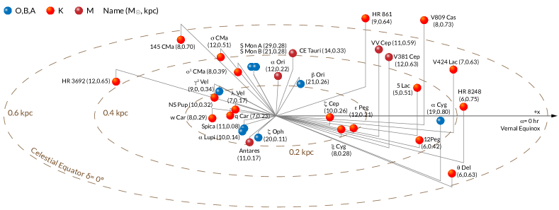
Figure 2: Illustration of nearby ($D\leq 1$ kpc) core collapse supernova candidates. Each star’s spectral type, name, mass and distance is shown in labels. See Table 6 for details and references.

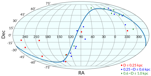
Figure 3: Mollweide projection of nearby ($D\leq 1$ kpc) core collapse supernova candidates. Symbols and colors correspond to distance intervals. The dotted line indicates the Galactic Plane. The red square near the center of the map is $\alpha$ Ori, best known as Betelgeuse.

2 Presupernova neutrino event rates and candidates

A liquid scintillator is ideal for the detection of presupernova neutrinos, through the inverse beta decay process (henceforth IBD, $\mathrel{{\bar{\nu}}_{e}}+p\rightarrow n+e^{+}$) due to its low energy threshold (1.8 MeV), and its timing, energy resolution, and background discrimination performance. The expected signal from a presupernova in neutrino detectors has been presented in recent articles (e.g., Asakura et al., 2016; Kato et al., 2015; Yoshida et al., 2016; Patton et al., 2017a; Kato et al., 2017; Li et al., 2020).

We consider an active detector mass of 17 kt, which is expected for JUNO, with detection efficiency of unity, and we use the IBD event rates in Patton et al. (2017a, 2019). Figure 1 shows the numbers of events and cumulative numbers of events for progenitor stars of zero age main-sequence (ZAMS) masses of 15 $\mathrel{{M_{\odot}}}$ and 30 $\mathrel{{M_{\odot}}}$ (here $\mathrel{{M_{\odot}}}=1.99\,10^{33}$ g is the mass of the Sun) at a distance of $D$=0.2 kpc (representative of Betelgeuse). Results are shown for the normal and inverted hierarchy of the neutrino mass spectrum. Times are negative, being relative to the time of core-collapse.

Figure 1 shows that a few hundred events are expected in the hours before core-collapse. For the 15 $\mathrel{{M_{\odot}}}$ model, the neutrino signal exceeds $\simeq$ 100 events at $t$=$-$4 hr and has a characteristic peak at $t\simeq-2.5$ hours, which marks the beginning of core silicon burning. For the 30 $\mathrel{{M_{\odot}}}$ model, the neutrino signal exceeds $\simeq$ 100 events at $t$=$-$2 hr. The number of events then increases steadily and rapidly, leading to a cumulative number of events that is larger than in the 15 $\mathrel{{M_{\odot}}}$ model.

For the detector background, we follow the event rates estimated in An et al. (2016) (see also Yoshida et al. (2016)) for JUNO: $r^{on}_{Bkg}\simeq 2.66/{\rm hr}$ and $r^{off}_{Bkg}\simeq 0.16/{\rm hr}$ in the reactor-on and reactor-off cases respectively. In addition to reactor neutrinos, other backgrounds are due, in comparable amounts (about 1 event per day each), to geoneutrinos, cosmogenic ⁸He/⁹Li, and accidental coincidences due to various radioactivity sources, like the natural decay chains, etc. For the latter, it is assumed that an effective muon veto will be in place, see An et al. (2016) for details. Roughly, a signal is detectable if the number of events expected is at least comparable with the number of background events in the same time interval ($N\gtrsim N_{\rm bkg}$). Using the reactor-on background rate, the most conservative presupernova event rate in Figure 1, and the fact that the number of signal events scales like $D^{-2}$, we estimate that a presupernova can be detected to a distance $D_{\rm max}\simeq$ 1 kpc.

What nearby stars could possibly undergo core collapse in the next few decades? To answer this question, we compiled a new list of 31 core collapse supernova candidates; see Appendix A and Table 6. Figure 2 gives an illustration of their names, positions, distances, masses, and colors. Figure 3 shows the equatorial coordinate system positions of the same stars, colored by distance bins, in a Mollweide projection. These candidates lie near the Galatic Plane, with clustering in directions associated with the Orion A molecular cloud (Großschedl et al., 2019) and the OB associations Cygnus OB2 and Carina OB1 (Lim et al., 2019). We find that for the stars in Table 6 the minimum separation (i.e., the separation of a star from its nearest neighbor in the same list) is, on average, $\langle\Delta\theta\rangle\simeq 10.4^{\circ}$, and that 70% of the candidate stars have $\Delta\theta\lesssim 12.8^{\circ}$ (see Table 7). Therefore, a sensitivity of $\simeq$ 10^∘ is desirable for complete disambiguation of the progenitor with a neutrino detector.

3 Angular Resolution and Sensitivity

Here we discuss the angular sensitivity of a liquid scintillator detector for realistic numbers of presupernova neutrino events. We consider two cases: a well tested liquid scintillator technology (henceforth LS) based on Linear AlkylBenzene (LAB), as is used in SNO+ (Andringa et al., 2016) and envisioned for JUNO; and a hypothetical setup where a Lithium compound is dissolved in the scintillator for enhanced angular sensitivity (henceforth LS-Li), as discussed for geoneutrino detection (Tanaka & Watanabe, 2014). As a notation definition, let us assume that the total number of events in the detector is $N=N_{S}+N_{\rm Bkg}$, where $N_{S}$ is the number of signal events and $N_{\rm Bkg}$ is the number of background events.

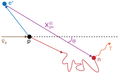
Figure 4: The geometry of Inverse Beta Decay in liquid scintillator. Shown are the incoming anti-neutrino (brown), proton (black), outgoing positron and its annihilation point (blue), outgoing neutron, its subsequent scattering events and its capture point (red), and the outgoing photon (orange). The vector $X^{(i)}_{pn}$ originates at the positron annihilation location and points in the direction of the neutron capture point. $\theta$ is the angle between $X^{(i)}_{pn}$ and the incoming neutrino momentum.

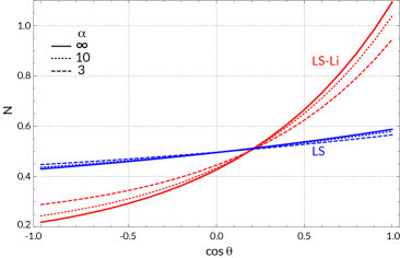
Figure 5: Normalized distributions of $\cos{\theta}$ for LS and LS-Li, for different values of the signal-to-background ratio, $\alpha=N_{S}/N_{\rm Bkg}$ (numbers in legend). Here, $\alpha=\infty$ means absence of background, $N_{\rm Bkg}=0$.

The IBD process in LS is illustrated in Figure 4. Overall, the sensitivity of this process to the direction of the incoming neutrino is moderate, with the emitted positron (neutron) momentum being slightly backward (forward)-distributed, see Beacom & Vogel (1999) and Vogel & Beacom (1999) for a detailed overview. Here, we follow the pointing method proposed and tested by the CHOOZ collaboration (Apollonio et al., 2000), which we describe briefly below.

Let us first consider a background-free signal, $N_{\rm Bkg}=0$. For each detected neutrino $\nu_{i}$ ($i=1,2,$…$,N$), we consider the unit vector $\hat{X}^{(i)}_{pn}$ that originates at the positron annihilation location and is directed towards the neutron capture point. Let $\theta$ be the angle that $\hat{X}^{(i)}_{pn}$ forms with the neutrino direction (see Figure 4). The unit vectors $\hat{X}^{(i)}_{pn}$ carry directional information – albeit with some degradation due to the neutron having to thermalize by scattering events before it can be captured – and possess a slightly forward distribution. The angular distributions expected for LS and LS-Li are given by Tanaka & Watanabe (2014) (in the context of geoneutrinos) in graphical form; we find that they are well reproduced by the following functions:

$$f_{LS}(\cos{\theta})\simeq 0.2718+0.2238\ \exp\left(0.345\cos{\theta}\right)$$ (1)

$$f_{LS-Li}(\cos{\theta})\simeq 0.1230+0.3041\ \exp\left(1.16\cos{\theta}\right).$$

Using these, one can find the forward-backward asymmetry, which is a measurable parameter:

$$\frac{a_{0}}{2}=\frac{N_{F}-N_{B}}{N_{F}+N_{B}}~{}.$$ (2)

Here $N_{F}$ and $N_{B}$ are the numbers of events in the forward ($\theta\leq\pi/2$) and backward ($\theta>\pi/2$) direction respectively. We obtain $a_{0}\simeq 0.16$ for LS, which is consistent with the distributions shown in Apollonio et al. (2000), and $a_{0}\simeq 0.78$ for LS-Li.

Let us now generalize to the case with a non-zero background, and define the signal-to-background ratio, $\alpha=N_{S}/N_{\rm Bkg}$. For simplicity, the background is modeled as isotropic and constant in time. Suppose that $N_{S}$, $\alpha$, and $a_{0}$ are known. In this case, the total angular distribution of the $N$ events will be a linear combination of two components, one for the directional signal

$$N_{B,S}=\frac{N_{S}}{2}\left(1-\frac{a_{0}}{2}\right)\qquad N_{F,S}=\frac{N_{S}}{2}\left(1+\frac{a_{0}}{2}\right),$$ (3)

and the other for the isotropic background

$$N_{B,{\rm Bkg}}=\frac{N_{\rm Bkg}}{2}\qquad N_{F,{\rm Bkg}}=\frac{N_{\rm Bkg}}{2}.$$ (4)

The two distributions have a relative weight of $\alpha$, which yields the forward-backward asymmetry as

$$\frac{a}{2}=\frac{(N_{F,S}+N_{F,{\rm Bkg}})-(N_{B,S}+N_{B,{\rm Bkg}})}{(N_{F,S}+N_{F,{\rm Bkg}})+(N_{B,S}+N_{B,{\rm Bkg}})}.$$ (5)

In the small background limit, $N_{\rm Bkg}\rightarrow 0$, then $\alpha\rightarrow\infty$ and $a\rightarrow a_{0}$. In the large background limit $N_{\rm Bkg}\rightarrow\infty$, then $\alpha\rightarrow 0$ and $a\rightarrow 0$.

Figure 5 shows the angular distribution for different signal-to-noise ratios $\alpha$ (see Table 1 for the corresponding values of $a$). For LS the $\alpha=\infty$ curve (blue solid) is taken from Equation (1), and for LS-Li the $\alpha=\infty$ curve (red solid) is taken from Equation (1). For LS-Li, an enhancement in the directionality is achieved as a result of an improved reconstruction of the positron annihilation point and a shortening of the neutron capture range. Enhancement in the directionality decreases for LS and LS-Li as the background becomes larger.

From here on, for all cases we adopt an approximate linear distribution for the $N$ events in the detector:

$$f(\cos{\theta})=\frac{1}{2}\Big{(}1+a\cos{\theta}\Big{)}~{}.$$ (6)

This form is accurate – yielding results that are commensurate with those obtained from the distributions in Figure 5 – and it allows to describe our results as functions of the varying parameter $a$ in a general and transparent manner.

Table 1: Values of $a$ for the curves in Figure 5.

$\alpha$	LS	LS-Li
$\infty$	0.1580	0.7820
10.0	0.1418	0.7165
3.0	0.1170	0.5911

Rigorously, $a$ depends on the neutrino energy. We investigated the uncertainty associated with treating $a$ as a (energy-independent) constant, and found it to be negligible in the present context where larger errors are present from, for example, uncertainties associated with modeling of the presupernova neutrino event rates. In addition, the values of $a$ used in the literature for supernova neutrinos, reactor neutrinos and geoneutrinos (e.g., Apollonio et al., 2000; Tanaka & Watanabe, 2014; Fischer et al., 2015) vary only by $\simeq$ 10-20% over a wide range of energy. The values of $a$ in Table 1 for the background-free $\alpha=\infty$ cases are used in Tanaka & Watanabe (2014) and Fischer et al. (2015) for geoneutrinos, which have an energy range ($E\simeq$ 2-5 MeV) and spectrum that is similar to those of presupernova neutrinos.

3.1 Pointing to the progenitor location

For a signal of $N$ IBD events in the detector from a point source on the sky, and therefore a set of unit vectors $\hat{X}^{(i)}_{pn}$ ($i=1,2,\ldots,N$), an estimate of the direction to the source is given by the average vector $\vec{p}$ (Apollonio et al., 2000; Fischer et al., 2015):

$$\vec{p}=\frac{1}{N}\sum_{i=1}^{N}\hat{X}^{(i)}_{pn}~{}.$$ (7)

This vector offers an immediate way to estimate the direction to the progenitor star in the sky. The calculation of the uncertainty in the direction is more involved (Apollonio et al., 2000), and requires examining the statistical distribution of $\vec{p}$, as follows.

Consider a Cartesian frame of reference where the neutrino source is on the negative side of the $z$-axis. In the limit of very high statistics ($N\rightarrow\infty$), the averages of the $x$- and $y$- components of the vectors $\hat{X}^{(i)}_{pn}$ vanish. The average of the $z$- component can be found from Equation (6), and is $\langle z\rangle=a/3$. Thus, the mean of $\vec{p}$ is:

$$\vec{p}_{m}=(0,0,|\vec{p}|)=(0,0,a/3)~{}.$$ (8)

For the linear distribution in Equation (6), the standard deviation is $\sigma=(\sqrt{3-a^{2}})/3\simeq 1/\sqrt{3}$ (where the approximation introduces a relative error of the form $a^{2}/6$, which is negligible in the present context). For $N\gg 1$, the Central Limit Theorem applies, and the distribution of the three components of $\vec{p}$ are Gaussians centered at the components of $\vec{p}_{m}$, and with standard deviations $\sigma_{x}=\sigma_{y}=\sigma_{z}=\sigma=1/\sqrt{3N}$. Hence, the probability distribution of the vector $\vec{p}$ is

$$P(p_{x},p_{y},p_{z})=\frac{1}{\big{(}2\pi\sigma^{2}\big{)}^{\frac{3}{2}}}\\ \exp\Bigg{(}\frac{-p_{x}^{2}-p_{y}^{2}-(p_{z}-|\vec{p}|)^{2}}{2\sigma^{2}}\Bigg{)}\;.$$ (9)

The angular uncertainty on the direction to the supernova progenitor is given by the angular aperture, $\beta$, of the cone around the vector $\vec{p}_{m}$, containing a chosen fraction of the total probability (e.g., $I=0.68$ or $I=0.90$):

$$\int P(p_{x},p_{y},p_{z})\ dp_{x}dp_{y}dp_{z}=I~{},$$ (10)

or, in spherical coordinates:

$$\int_{0}^{\infty}p^{2}dp\int_{\cos{\beta}}^{1}d\cos{\theta}\int_{0}^{2\pi}d\phi\ P(p_{x},p_{y},p_{z})=I~{}.$$ (11)

The latter form reduces to:

$$\frac{1}{2}\Bigg{[}1+{\rm Erf}(k)-\cos{\beta}\ \exp{\Bigg{(}-k^{2}\sin^{2}{\beta}\Bigg{)}}\\ \bigg{(}1+{\rm Erf}(k\cos{\beta})\bigg{)}\Bigg{]}=I\;,$$ (12)

where $k=\sqrt{3N/2}~{}|\vec{p}|=a\sqrt{N/6}$, and the error function is ${\rm Erf}(z)=2/\sqrt{\pi}\int_{0}^{z}\exp(-t^{2})\ dt$.

For a fixed value of $I$, Equation (12) can be solved numerically to find $\beta=\beta(k,I)$, and therefore to reveal the dependence of $\beta$ on $N$ and $a$. Figure 6 shows the dependence of $\beta$ on $N$, for two confidence levels (C.L.). The figure illustrates the (expected) poor performance of LS: we have $\beta\simeq 70^{\circ}$ at 68% C.L. and $N=100$, improving to $\beta\simeq 40^{\circ}$ at $N=500$. For the same C.L. and values of $N$, LS-Li would allow an improvement in the error by nearly a factor of 4, giving $\beta\simeq 18^{\circ}$ and $\beta\simeq 10^{\circ}$ in the two cases respectively. The degree of improvement in performance with increasing $a$ is shown in Figure 7, where $N=200$ is kept fixed.

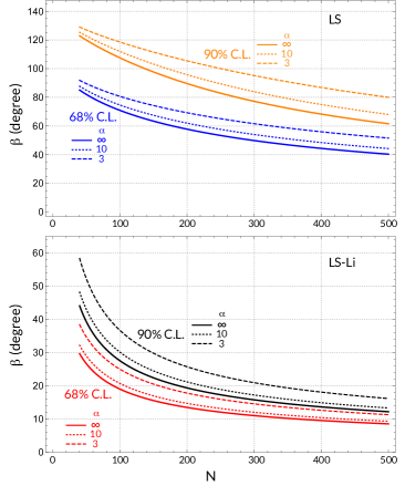
Figure 6: The angular uncertainty, $\beta$, as a function of the number of events, for LS and LS-Li, two different confidence levels, and three values of the signal-to-background ratio, $\alpha$ (see figure legend).

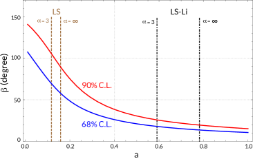
Figure 7: The angular uncertainty, $\beta$, as a function of the forward-backward asymmetry, $a$, for two different confidence levels (see figure legend) and fixed number of events, $N=200$. The vertical lines indicate the values of $a$ corresponding to $\alpha=\infty,~{}3$ for LS (dashed lines) and LS-Li (dot-dashed), see Table 1.

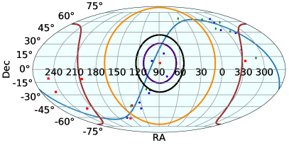
(a) t = -4.0 hours

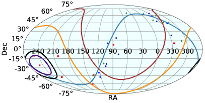
(b) t = -4.0 hours

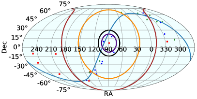
(c) t = -1.0 hour

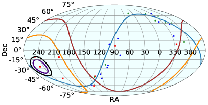
(d) t = -1.0 hour

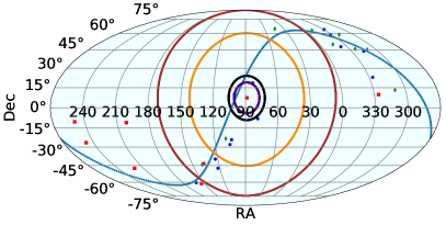
(e) t = -2 minutes

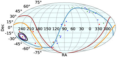
(f) t = -2 minutes

Figure 8: Angular error cones at 68% C.L. and 90% C.L. for LS (orange and maroon contours), and LS-Li (indigo and black contours) at 4 hours, 1 hour and 2 minutes prior to the core collapse. The left panels correspond to Betelgeuse ($D$= 0.222 kpc, $M\simeq 15\mathrel{{M_{\odot}}}$); the right panels to Antares ($D$= 0.169 kpc, $M\simeq 15\mathrel{{M_{\odot}}}$). The presence of background is considered in all cases according to An et al. (2016). The number of events is based on the model by Patton et al. (2017b).

Figure 9: Same as Figure 8, but for $\sigma$ Canis Majoris (left panels, $D$= 0.513 kpc, $M\simeq 15\mathrel{{M_{\odot}}}$) and S Monocerotis A (right panels, $D$= 0.282 kpc, $M\simeq 30\mathrel{{M_{\odot}}}$). Only 68% C.L. contours are shown here, for LS (orange) and LS-Li (indigo).

In the case of isotropic background the mean vector, $\vec{p}_{m}$, still points in the direction of the progenitor star. That is no longer true in the general case of anisotropic background, which would introduce a systematic shift in the direction of $\vec{p}_{m}$. A naive estimate for a point-like source of background gives an (average) shift in direction by an angle $\delta\lesssim N_{Bkg}/N_{S}$ (valid if $N_{Bkg}\ll N_{S}$ and independent of $a$), corresponding to $\delta\lesssim 4^{\circ}-10^{\circ}$ for parameters typical of Betelgeuse (see Table 2). A comparison with the typical values of $\beta$ indicates that the shift is probably negligible for LS ($\beta\gg\delta$, typically) but might have to be considered for LS-Li. A more accurate estimate of $\delta$ depends on site-specific information and is beyond the scope of the present paper.

Another source of potential uncertainty is in the site-specific number of accidental coincidences in the detector (e.g., a coincidence between a positron from a cosmic muon decay and a neutron capture from a different process). Although here we assume a strong muon veto (An et al., 2016), the actual performance of the veto in a realistic setting may be different and contribute to larger background levels that would negatively affect the presupernova localization. See Cao & Wang (2017) and references therein for technical information on realistic veto designs and their expected performance.

4 Progenitor Identification

Attempts at progenitor identification will involve a complex interplay of different information from different channels. Here, we discuss a plausible, although simplified, scenario where two essential elements are combined: (i) pointing information from a single liquid scintillator detector, using the method in Section 3; and (ii) a rough estimate of the distance to the star, from the comparison of the signal with models . Both these indicators will evolve with time over the duration of the presupernova signal, with the list of plausible candidates becoming shorter as higher statistics are collected in the detector. We emphasize that the goal here is not necessarily to reduce to a single star; even reducing the list to a few stars (3 or 4, for example) can be useful to the gravitational wave and electromagnetic astronomy communities.

Consider the two case studies shown in Figure 8 and detailed in Tables 2 and 3. The left column refers to Betelgeuse and the right column to Antares, both with a time distribution of IBD events as in Figure 1 for 15 $\mathrel{{M_{\odot}}}$. The three panels show how the 68% and 90% C.L. angular errors decrease with time, leading to a progressively more accurate estimate of the position.

For the case of LS, at $t=-1$ hr pre-collapse, as many as $\sim$ 10 progenitor stars are within the angular error cone, with only a minimal improvement at later times. Therefore, the identification of the progenitor can not be achieved using the angular information alone. It might be possible, however, in the presence of a rough distance estimation from the event rate in the detector. In both examples, a possible upper limit of $D<0.25$ kpc (red squares in Figure 8, also see Figure 3) results in a single pre-supernova being favored. For LS-Li, the angular information alone is sufficient to favor 3-4 stars as likely progenitors already $\sim$4 hours pre-collapse. At $t=-1$ hr, a single progenitor can be identified in the case of Antares.

A less fortunate scenario is shown in the left panels in Figure 9 (details in Table 4) for $\sigma$ Canis Majoris (distance $D=0.513$ kpc). The number of events was calculated according to the $15\mathrel{{M_{\odot}}}$ model in Figure 1. The lower signal statistics (the number of events barely reaches 60), and the larger relative importance of the background result in a decreased angular sensitivity. We find that LS will only eliminate roughly half of the sky if we use the 68% C.L. error cone. When combined with an approximate distance estimate, this coarse angular information might lead to identifying $\sim$ 10 stars as potential candidates. With LS-Li, the list of candidates might be slightly shorter but a unique identification would be very unlikely, even immediately before collapse.

A 30 $\mathrel{{M_{\odot}}}$ case is represented by the right panels in Figure 9 (and detailed in Table 5) for S Monocerotis A (distance $D=0.282$ kpc). An hour prior to the collapse $\simeq$  120 events are expected, allowing LS to shorten the progenitor list to $\simeq$ 12 stars within the error cone at $68\%$ C.L. Whereas, LS-Li narrows the progenitor list down to $\simeq$ 3 stars with the same C.L. one hour prior to the collapse. When combined with a rough distance estimate, the progenitor might be successfully identified.

In closing of this section, let us elaborate on the potential of estimating the distance to the star by comparing the observed neutrino event rate with models. The accuracy of such estimate depends on the uncertainty on model predictions, which in principle can be estimated from the spread in the presupernova neutrino number luminosity from different models in the current literature that begin with the same zero-age main sequence mass. Unfortunately, the presupernova models in the present literature do not allow a reasonable direct comparison due to key, yet often undisclosed, modelling choices made during the evolution of a stellar model (although see Patton et al. (2017b) for an exception). For example, the neutrino number luminosity can change by more than an order of magnitude due to the prescription used for mass loss by stellar winds over the evolution of the model, the treatment of convective boundaries, the spatial (mass) and temporal resolution of the model over its evolution, the global conservation of energy by the model over its evolution, the number of isotopes evolved by the nuclear reaction network, and how nuclear burning is coupled to the hydrodynamics (operator split versus fully coupled vs post-processing) especially during the advanced stages of massive star evolution. We must conclude, therefore, that the idea to use models to place distance constraints will become realistic only in the future, after more progress is achieved on presupernova emission models.

5 Discussion

We have demonstrated that it will be possible to use the neutrino IBD signal at a large liquid scintillator detector to obtain an early localization of a nearby pre-supernova ($D\lesssim 1$ kpc). The method we propose is robust, as it has been used successfully for reactor neutrinos, and it is sufficiently simple that it can be implemented during a pre-supernova signal detection. For a detector where the forward-backward asymmetry is about 10% (realistic for JUNO), and 200 events detected (also realistic at JUNO, for a star like Betelgeuse) the angular resolution is $\beta\simeq 60^{\circ}$, which is moderate, but sufficient to exclude a large number of potential candidate progenitors.

The method has the potential to become even more sensitive if it is used with LS-Li, and therefore it provides further motivation to develop new experimental concepts in this direction. For example, 200 signal events with forward-backward asymmetry of $\sim$40% would result in a resolution of about $15^{\circ}$, and the possibility to uniquely identify the progenitor star.

In a realistic situation, as soon as a presupernova signal is detected with high confidence (a few tens of candidate events), an alert with a coarse localization information can be issued, followed by updates with improved angular resolution in the minutes or hours leading to the neutrino burst detection.

Using the Patton et al. (2017b) presupernova model, we find that (see Figure 8) when the number of events reaches $N=100$ ($\simeq$ 1 hour pre-collapse for Betelgeuse), the angular information is already close to optimal, since only a minimal improvement of the positional estimate can be gained at subsequent times. Note, however, that our results are conservative. According to other simulations where the presupernova neutrino luminosity reaches a detectable level over a time scale of days (Kato et al., 2015; Guo et al., 2019), it might be possible to detect a larger number of events, resulting in even better angular resolutions in the last 1-2 hours before the core collapse.

It is possible that, when a nearby star reaches its final day or hours before becoming a supernova, a new array of neutrino detectors will be available. A large liquid scintillator experiment like the proposed THEIA (Askins et al., 2019), which could reach 80 kt (fiducial) mass, could observe more than $10^{3}$ IBD events, with an angular resolution of at least $\sim 30^{\circ}$. The resolution of THEIA would be improved by using a water-based liquid scintillator, where the capability to separate the scintillation and Cherenkov light would result in enhanced pointing ability (e.g., Askins et al., 2019) for IBD, and in the possibility to use neutrino-electron elastic scattering for pointing. A subdominant, but still useful, contribution to the pointing effort – at the level of tens of events – will come from $\mathcal{O}(1)$ kt liquid scintillator projects like SNO+ (Andringa et al., 2016) and the Jinping Neutrino Experiment (Beacom et al., 2017), for which the deep underground depth will result in very low background levels. Further activities on directionality in scintillators are ongoing (e.g., Biller et al., 2020). Data from elastic scattering events at water Cherenkov detectors like SuperKamiokande (Simpson et al., 2019) and possibly the planned HyperKamiokande ($\mathcal{O}(100)$ kt) (Abe et al., 2016), will also contribute, despite the loss of statistics (compared to liquid scintillator) due to the higher energy threshold ($\sim 5-7$ MeV). In these detectors, a possible phase with Gadolinium dissolved in the water, like in the upcoming SuperK-Gd, (Beacom & Vagins, 2004; Simpson et al., 2019), will allow better discrimination of the IBD events, resulting in an enhanced pointing potential.

In addition to new experimental scenarios, a different theoretical panorama may be realized as well, and there might be novel avenues to conduct fundamental science tests (e.g., searches for exotic light and weakly interacting particles) using presupernova neutrinos.

Table 2: Parameters and results for Betelgeuse, Figure 8, left panels. The angular errors at a given confidence level (C.L.) are in degrees.

					LS			LS-Li
Time to CC	$N_{\rm Total}$	$N_{\rm Signal}$	$N_{\rm Bkg}$	$\alpha$	$a$	68% C.L.	90% C.L.	$a$	68% C.L.	90% C.L.
4.0 hr	93	78	15	5.20	0.1308	$78.43^{\circ}$	$116.17^{\circ}$	0.6610	$23.24^{\circ}$	$33.98^{\circ}$
1.0 hr	193	170	23	7.39	0.1374	$63.92^{\circ}$	$98.42^{\circ}$	0.6942	$15.47^{\circ}$	$22.26^{\circ}$
2 min	314	289	25	11.56	0.1435	$52.72^{\circ}$	$81.79^{\circ}$	0.7254	$11.63^{\circ}$	$16.67^{\circ}$

Table 3: Parameters and results for Antares, Figure 8, right panels.

					LS			LS-Li
Time to CC	$N_{\rm Total}$	$N_{\rm Signal}$	$N_{\rm Bkg}$	$\alpha$	$a$	68% C.L.	90% C.L.	$a$	68% C.L.	90% C.L.
4.0 hr	161	146	15	9.73	0.1414	$66.27^{\circ}$	$101.59^{\circ}$	0.7147	$16.44^{\circ}$	$23.70^{\circ}$
1.0 hr	333	310	23	13.48	0.1452	$51.11^{\circ}$	$79.24^{\circ}$	0.7337	$11.16^{\circ}$	$15.98^{\circ}$
2 min	543	518	25	20.72	0.1488	$41.02^{\circ}$	$62.70^{\circ}$	0.7519	$8.54^{\circ}$	$12.19^{\circ}$

Table 4: Parameters and results for $\sigma$ Canis Majoris, Figure 9, left panels.

					LS		LS-Li
Time to CC	$N_{\rm Total}$	$N_{\rm Signal}$	$N_{\rm Bkg}$	$\alpha$	$a$	68 % C.L.	$a$	68 % C.L.
2.0 hr	31	11	20	0.55	0.0553	$103.28^{\circ}$	0.2797	$71.43^{\circ}$
1.0 hr	36	13	23	0.56	0.0560	$102.54^{\circ}$	0.2829	$68.32^{\circ}$
2 min	58	33	25	1.32	0.0887	$93.56^{\circ}$	0.4484	$41.57^{\circ}$

Table 5: Parameters and results for S Monocerotis A, Figure 9, right panels.

					LS		LS-Li
Time to CC	$N_{\rm Total}$	$N_{\rm Signal}$	$N_{\rm Bkg}$	$\alpha$	$a$	68 % C.L.	$a$	68 % C.L.
2.0 hr	44	24	20	1.20	0.0850	$96.53^{\circ}$	0.4300	$48.26^{\circ}$
1.0 hr	141	118	23	5.13	0.1305	$71.60^{\circ}$	0.6596	$19.00^{\circ}$
2 min	420	395	25	15.80	0.1466	$46.28^{\circ}$	0.7413	$9.84^{\circ}$

Appendix A Pre-Supernova Candidates

Table 6 compiles a list of 31 red and blue core-collapse supernova progenitors within 1 kpc that have both distance and mass estimates. Table 6 gives the star number (sorted by distance), Henry Draper (HD) catalog number, common name, constellation, distance, mass, J2000 right ascension (RA) and J2000 declination (Dec). For stars with multiple distance measurements, precedence is given to distances provided by the Gaia Collaboration et al. (2018), van Leeuwen (2007), and individual determinations, in this order. Earlier compilations (e.g., Nakamura et al., 2016) considered only red supergiant progenitors and did not require a mass estimate.

Table 7 lists the angular distance $\Delta\theta$ of each star to its nearest neighbor. Table 7 gives the star number, HD catalog and common name, the minimum angular separation between the star and its nearest neighbor, the HD catalog and common name of the nearest neighbor, and the star number of the nearest neighbor. The RA and Dec for each star is taken from Table 6 when calculating angular separations.

Table 6: Candidate Pre-supernova Stars.

N	Catalog Name	Common Name	Constellation	Distance (kpc)	Mass (M⊙)	RA	Dec
1	HD 116658	Spica/$\alpha$ Virginis	Virgo	$0.077\pm 0.004$	$11.43^{+1.15}_{-1.15}$	13:25:11.58	$-$11:09:40.8
2	HD 149757	$\zeta$ Ophiuchi	Ophiuchus	$0.112\pm 0.002$	$20.0$	16:37:09.54	$-$10:34:01.53
3	HD 129056	$\alpha$ Lupi	Lupus	$0.143\pm 0.003$	$10.1^{+1.0}_{-1.0}$	14:41:55.76	$-$47:23:17.52
4	HD 78647	$\lambda$ Velorum	Vela	$0.167\pm 0.003$	$7.0^{+1.5}_{-1.0}$	09:07:59.76	$-$43:25:57.3
5	HD 148478	Antares/$\alpha$ Scorpii	Scorpius	$0.169\pm 0.030$	$11.0-14.3$	16:29:24.46	$-$26:25:55.2
6	HD 206778	$\epsilon$ Pegasi	Pegasus	$0.211\pm 0.006$	$11.7^{+0.8}_{-0.8}$	21:44:11.16	+09:52:30.0
7	HD 39801	Betelgeuse/$\alpha$ Orionis	Orion	$0.222\pm 0.040$	$11.6^{+5.0}_{-3.9}$	05:55:10.31	+07:24:25.4
8	HD 89388	q Car/V337 Car	Carina	$0.230\pm 0.020$	$6.9^{+0.6}_{-0.6}$	10:17:04.98	$-$61:19:56.3
9	HD 210745	$\zeta$ Cephei	Cepheus	$0.256\pm 0.006$	$10.1^{+0.1}_{-0.1}$	22:10:51.28	+58:12:04.5
10	HD 34085	Rigel/$\beta$ Orion	Orion	$0.264\pm 0.024$	$21.0^{+3.0}_{-3.0}$	05:14:32.27	$-$08:12:05.90
11	HD 200905	$\xi$ Cygni	Cygnus	$0.278\pm 0.029$	$8.0$	21:04:55.86	+43:55:40.3
12	HD 47839	S Monocerotis A	Monoceros	$0.282\pm 0.040$	$29.1$	06:40:58.66	+09:53:44.71
13	HD 47839	S Monocerotis B	Monoceros	$0.282\pm 0.040$	$21.3$	06:40:58.57	+09:53:42.20
14	HD 93070	w Car/V520 Car	Carina	$0.294\pm 0.023$	$7.9^{+0.1}_{-0.1}$	10:43:32.29	$-$60:33:59.8
15	HD 68553	NS Puppis	Puppis	$0.321\pm 0.032$	$9.7$	08:11:21.49	$-$39:37:06.8
16	HD 36389	CE Tauri/119 Tauri	Taurus	$0.326\pm 0.070$	$14.37^{+2.00}_{-2.77}$	05:32:12.75	+18:35:39.2
17	HD 68273	$\gamma^{2}$ Velorum	Vela	$0.342\pm 0.035$	$9.0^{+0.6}_{-0.6}$	08:09:31.95	$-$47:20:11.71
18	HD 50877	$o^{1}$ Canis Majoris	Canis Major	$0.394\pm 0.052$	$7.83^{+2.0}_{-2.0}$	06:54:07.95	$-$24:11:03.2
19	HD 207089	12 Pegasi	Pegasus	$0.415\pm 0.031$	$6.3^{+0.7}_{-0.7}$	21:46:04.36	+22:56:56.0
20	HD 213310	5 Lacertae	Lacerta	$0.505\pm 0.046$	$5.11^{+0.18}_{-0.18}$	22:29:31.82	+47:42:24.8
21	HD 52877	$\sigma$ Canis Majoris	Canis Major	$0.513\pm 0.108$	$12.3^{+0.1}_{-0.1}$	07:01:43.15	$-$27:56:05.4
22	HD 208816	VV Cephei	Cepheus	$0.599\pm 0.083$	$10.6^{+1.0}_{-1.0}$	21:56:39.14	+63:37:32.0
23	HD 196725	$\theta$ Delphini	Delphinus	$0.629\pm 0.029$	$5.60^{+3.0}_{-3.0}$	20:38:43.99	+13:18:54.4
24	HD 203338	V381 Cephei	Cepheus	$0.631\pm 0.086$	$12.0$	21:19:15.69	+58:37:24.6
25	HD 216946	V424 Lacertae	Lacerta	$0.634\pm 0.075$	$6.8^{+1.0}_{-1.0}$	22:56:26.00	+49:44:00.8
26	HD 17958	HR 861	Cassiopeia	$0.639\pm 0.039$	$9.2^{+0.5}_{-0.5}$	02:56:24.65	+64:19:56.8
27	HD 80108	HR 3692	Vela	$0.650\pm 0.061$	$12.1^{+0.2}_{-0.2}$	09:16:23.03	-44:15:56.6
28	HD 56577	145 Canis Major	Canis Major	$0.697\pm 0.078$	$7.8^{+0.5}_{-0.5}$	07:16:36.83	$-$23:18:56.1
29	HD 219978	V809 Cassiopeia	Cassiopeia	$0.730\pm 0.074$	$8.3^{+0.5}_{-0.5}$	23:19:23.77	+62:44:23.2
30	HD 205349	HR 8248	Cygnus	$0.746\pm 0.039$	$6.3^{+0.7}_{-0.7}$	21:33:17.88	+45:51:14.5
31	HD 102098	Deneb/$\alpha$ Cygni	Cygnus	$0.802\pm 0.066$	$19.0^{+4.0}_{-4.0}$	20:41:25.9	+45:16:49.0

Note. — ^avan Leeuwen (2007), ^bTkachenko et al. (2016), ^cGaia Collaboration et al. (2018), ^dHarper et al. (2017), ^eSchiller & Przybilla (2008), ^fTetzlaff et al. (2011), ^gHowarth & Smith (2001), ^hCarpenter et al. (1999), ⁱCvetkovic et al. (2009), ^jShultz et al. (2014), ^kMontargès et al. (2018), ^lOhnaka et al. (2013), ^mNeilson et al. (2011), ⁿvan Belle et al. (2009); Malagnini et al. (2000), ^oNorth et al. (2007), ^pLee et al. (2014), ^qBaines et al. (2018), ^rReimers & Schroeder (1989), ^sTokovinin (1997)

Table 7: Minimum Angular Separation Between Pre-supernova Candidates.

N	Catalog/Common	Min. Ang.	Nearest Neighbor	Nearest Neighbor
	Name	Separation (degree)	Name	Number
1	HD 116658/Spica	39.66	HD 129056/$\alpha$ Lupi	3
2	HD 149757/$\zeta$ Ophiuchi	15.97	HD 148478/Antares	5
3	HD 129056/$\alpha$ Lupi	29.73	HD 148478/Antares	5
4	HD 78647/$\lambda$ Velorum	1.73	HD 80108/HR 3692	27
5	HD 148478/Antares	15.97	HD 149757/$\zeta$ Ophiuchi	2
6	HD 206778/$\epsilon$ Pegasi	13.08	HD 207089/12 Pegasi	19
7	HD 39801/Betelgeuse	11.59	S Mono A/B	12/13
8	HD 89338/q Car	3.30	HD 93070/w Car	14
9	HD 210745/$\zeta$ Cephei	5.69	HD 208816/VV Cephei	22
10	HD 34085/Rigel	18.60	HD 39801/Betelgeuse	7
11	HD 200905/$\zeta$ Cygni	4.39	HD 102098/Deneb	31
12	HD 47839/S Mono A	11.60	HD 39801/Betelgeuse	7
13	HD 47839/S Mono B	11.60	HD 39801/Betelgeuse	7
14	HD 93070/w Car	3.30	HD 89338/q Car	8
15	HD 68553/NS Puppis	7.72	HD 68273/$\gamma^{2}$ Velorum	17
16	HD 36389/119 Tauri	12.50	HD 39801/Betelgeuse	7
17	HD 68273/$\gamma^{2}$ Velorum	7.72	HD 68553/NS Puppis	15
18	HD 50877/$o^{1}$ Canis Majoris	4.12	HD 52877/$\sigma$ Canis Majoris	21
19	HD 207089/12 Pegasi	13.08	HD 206778/$\epsilon$ Pegasi	6
20	HD 213310/5 Lacertae	4.88	HD 216946/V424 Lacertae	25
21	HD 52877/$\sigma$ Canis Majoris	4.12	HD 50877/$o^{1}$ Canis Majoris	18
22	HD 208816/VV Cephei	5.69	HD 210745/$\zeta$ Cephei	9
23	HD 196725/$\theta$ Delphini	16.39	HD 206778/$\epsilon$ Pegasi	6
24	HD 203338/V381 Cephei	6.72	HD 208816/VV Cephei	22
25	HD 216946/V424 Lacertae	4.88	HD 213310/5 Lacertae	20
26	HD 17958/HR 861	23.49	HD 219978/V809 Cassiopeia	29
27	HD 80108/HR 3692	1.73	HD 78647/$\lambda$ Velorum	4
28	HD 56577/145 Canis Majoris	5.22	HD 50877/$o^{1}$ Canis Majoris	18
29	HD 219978/V809 Cassiopeia	9.33	HD 208816/VV Cephei	22
30	HD 205349/HR 8248	5.38	HD 200905/$\zeta$ Cygni	11
31	HD 102098/Deneb	4.39	HD 200905/$\zeta$ Cygni	11

References

- Aalbers et al. (2016) Aalbers, J., Agostini, F., Alfonsi, M., et al. 2016, J. Cosmology Astropart. Phys, 2016, 017, doi: 10.1088/1475-7516/2016/11/017
- Aalseth et al. (2018) Aalseth, C. E., Acerbi, F., Agnes, P., et al. 2018, European Physical Journal Plus, 133, 131, doi: 10.1140/epjp/i2018-11973-4
- Abe et al. (2016) Abe, K., Haga, Y., Hayato, Y., et al. 2016, Astroparticle Physics, 81, 39, doi: 10.1016/j.astropartphys.2016.04.003
- Acciarri et al. (2016) Acciarri, R., et al. 2016, arXiv e-prints. https://arxiv.org/abs/1601.02984
- Alekseev et al. (1987) Alekseev, E. N., Alekseeva, L. N., Volchenko, V. I., & Krivosheina, I. V. 1987, Soviet Journal of Experimental and Theoretical Physics Letters, 45, 589
- An et al. (2016) An, F., An, G., An, Q., et al. 2016, Journal of Physics G Nuclear Physics, 43, 030401, doi: 10.1088/0954-3899/43/3/030401
- Andringa et al. (2016) Andringa, S., et al. 2016, Adv. High Energy Phys., 2016, 6194250, doi: 10.1155/2016/6194250
- Antonioli et al. (2004) Antonioli, P., Tresch Fienberg, R., Fleurot, R., et al. 2004, New Journal of Physics, 6, 114, doi: 10.1088/1367-2630/6/1/114
- Apollonio et al. (2000) Apollonio, M., Baldini, A., Bemporad, C., et al. 2000, Phys. Rev. D, 61, 012001, doi: 10.1103/PhysRevD.61.012001
- Araki et al. (2005) Araki, T., et al. 2005, Phys. Rev. Lett., 94, 081801, doi: 10.1103/PhysRevLett.94.081801
- Asakura et al. (2016) Asakura, K., Gando, A., Gando, Y., et al. 2016, ApJ, 818, 91, doi: 10.3847/0004-637X/818/1/91
- Askins et al. (2019) Askins, M., et al. 2019, arXiv e-prints. https://arxiv.org/abs/1911.03501
- Baines et al. (2018) Baines, E. K., Armstrong, J. T., Schmitt, H. R., et al. 2018, AJ, 155, 30, doi: 10.3847/1538-3881/aa9d8b
- Beacom & Vagins (2004) Beacom, J. F., & Vagins, M. R. 2004, Phys. Rev. Lett., 93, 171101, doi: 10.1103/PhysRevLett.93.171101
- Beacom & Vogel (1999) Beacom, J. F., & Vogel, P. 1999, Phys. Rev. D, 60, 033007, doi: 10.1103/PhysRevD.60.033007
- Beacom et al. (2017) Beacom, J. F., et al. 2017, Chin. Phys., C41, 023002, doi: 10.1088/1674-1137/41/2/023002
- Beaudet et al. (1967) Beaudet, G., Petrosian, V., & Salpeter, E. E. 1967, ApJ, 150, 979, doi: 10.1086/149398
- Biller et al. (2020) Biller, S. D., Leming, E. J., & Paton, J. L. 2020, arXiv e-prints. https://arxiv.org/abs/2001.10825
- Bionta et al. (1987) Bionta, R. M., Blewitt, G., Bratton, C. B., et al. 1987, Phys. Rev. Lett., 58, 1494, doi: 10.1103/PhysRevLett.58.1494
- Bisnovatyi-Kogan & Seidov (1984) Bisnovatyi-Kogan, G. S., & Seidov, Z. F. 1984, Annals of the New York Academy of Sciences, 422, 319, doi: 10.1111/j.1749-6632.1984.tb23362.x
- Borexino Collaboration et al. (2018) Borexino Collaboration, Agostini, M., Altenmüller, K., et al. 2018, Nature, 562, 505, doi: 10.1038/s41586-018-0624-y
- Brugière (2017) Brugière, T. 2017, Nuclear Instruments and Methods in Physics Research A, 845, 326, doi: 10.1016/j.nima.2016.05.111
- Cao & Wang (2017) Cao, L. J., & Wang, Y. 2017, Ann. Rev. Nucl. Part. Sci., 67, 183, doi: 10.1146/annurev-nucl-101916-123318
- Carpenter et al. (1999) Carpenter, K. G., Robinson, R. D., Harper, G. M., et al. 1999, ApJ, 521, 382, doi: 10.1086/307520
- Cvetkovic et al. (2009) Cvetkovic, Z., Vince, I., & Ninkovic, S. 2009, Publications de l’Observatoire Astronomique de Beograd, 86, 331
- Farag et al. (2020) Farag, E., Timmes, F. X., Taylor, M., Patton, K. M., & Farmer, R. 2020, arXiv e-prints, arXiv:2003.05844. https://arxiv.org/abs/2003.05844
- Fischer et al. (2015) Fischer, V., Chirac, T., Lasserre, T., et al. 2015, J. Cosmology Astropart. Phys, 2015, 032, doi: 10.1088/1475-7516/2015/08/032
- Fowler & Hoyle (1964) Fowler, W. A., & Hoyle, F. 1964, ApJS, 9, 201, doi: 10.1086/190103
- Fuller et al. (1980) Fuller, G. M., Fowler, W. A., & Newman, M. J. 1980, ApJS, 42, 447
- Fuller et al. (1982a) —. 1982a, ApJS, 48, 279, doi: 10.1086/190779
- Fuller et al. (1982b) —. 1982b, ApJ, 252, 715, doi: 10.1086/159597
- Fuller et al. (1985) —. 1985, ApJ, 293, 1, doi: 10.1086/163208
- Gaia Collaboration et al. (2018) Gaia Collaboration, Brown, A. G. A., Vallenari, A., et al. 2018, A&A, 616, A1, doi: 10.1051/0004-6361/201833051
- Großschedl et al. (2019) Großschedl, J. E., Alves, J., Teixeira, P. S., et al. 2019, A&A, 622, A149, doi: 10.1051/0004-6361/201832577
- Guo et al. (2019) Guo, G., Qian, Y.-Z., & Heger, A. 2019, Phys. Lett., B796, 126, doi: 10.1016/j.physletb.2019.07.030
- Guo et al. (2007) Guo, X., et al. 2007, arXiv e-prints. https://arxiv.org/abs/hep-ex/0701029
- Harper et al. (2017) Harper, G. M., Brown, A., Guinan, E. F., et al. 2017, AJ, 154, 11, doi: 10.3847/1538-3881/aa6ff9
- Hirata et al. (1987) Hirata, K., Kajita, T., Koshiba, M., Nakahata, M., & Oyama, Y. 1987, Phys. Rev. Lett., 58, 1490, doi: 10.1103/PhysRevLett.58.1490
- Hirata et al. (1988) Hirata, K. S., Kajita, T., Koshiba, M., et al. 1988, Phys. Rev. D, 38, 448, doi: 10.1103/PhysRevD.38.448
- Howarth & Smith (2001) Howarth, I. D., & Smith, K. C. 2001, MNRAS, 327, 353, doi: 10.1046/j.1365-8711.2001.04658.x
- Hunter (2007) Hunter, J. D. 2007, Computing in Science & Engineering, 9, 90, doi: 10.1109/MCSE.2007.55
- IceCube Collaboration et al. (2018a) IceCube Collaboration, Aartsen, M. G., Ackermann, M., et al. 2018a, Science, 361, eaat1378, doi: 10.1126/science.aat1378
- IceCube Collaboration et al. (2018b) —. 2018b, Science, 361, 147, doi: 10.1126/science.aat2890
- Itoh et al. (1996) Itoh, N., Hayashi, H., Nishikawa, A., & Kohyama, Y. 1996, ApJS, 102, 411
- Kato et al. (2015) Kato, C., Delfan Azari, M., Yamada, S., et al. 2015, ApJ, 808, 168, doi: 10.1088/0004-637X/808/2/168
- Kato et al. (2017) Kato, C., Nagakura, H., Furusawa, S., et al. 2017, ApJ, 848, 48, doi: 10.3847/1538-4357/aa8b72
- Krauss et al. (1984) Krauss, L. M., Glashow, S. L., & Schramm, D. N. 1984, Nature, 310, 191, doi: 10.1038/310191a0
- Kutschera et al. (2009) Kutschera, M., Odrzywołek, A., & Misiaszek, M. 2009, Acta Physica Polonica B, 40, 3063
- Kyutoku & Kashiyama (2018) Kyutoku, K., & Kashiyama, K. 2018, Phys. Rev. D, 97, 103001, doi: 10.1103/PhysRevD.97.103001
- Langanke & Martínez-Pinedo (2000) Langanke, K., & Martínez-Pinedo, G. 2000, Nuclear Physics A, 673, 481, doi: 10.1016/S0375-9474(00)00131-7
- Langanke & Martínez-Pinedo (2014) —. 2014, Nuclear Physics A, 928, 305, doi: 10.1016/j.nuclphysa.2014.04.015
- Lee et al. (2014) Lee, B. C., Han, I., Park, M. G., Hatzes, A. P., & Kim, K. M. 2014, A&A, 566, A124, doi: 10.1051/0004-6361/201321863
- Li et al. (2020) Li, H.-L., Li, Y.-F., Wen, L.-J., & Zhou, S. 2020, arXiv e-prints, arXiv:2003.03982. https://arxiv.org/abs/2003.03982
- Li (2014) Li, Y.-F. 2014, in International Journal of Modern Physics Conference Series, Vol. 31, International Journal of Modern Physics Conference Series, 1460300, doi: 10.1142/S2010194514603007
- Lim et al. (2019) Lim, B., Nazé, Y., Gosset, E., & Rauw, G. 2019, MNRAS, 490, 440, doi: 10.1093/mnras/stz2548
- Lin & Lunardini (2020) Lin, Z., & Lunardini, C. 2020, Phys. Rev., D101, 023016, doi: 10.1103/PhysRevD.101.023016
- Malagnini et al. (2000) Malagnini, M. L., Morossi, C., Buzzoni, A., & Chavez, M. 2000, PASP, 112, 1455, doi: 10.1086/317714
- Misch et al. (2018) Misch, G. W., Sun, Y., & Fuller, G. M. 2018, ApJ, 852, 43, doi: 10.3847/1538-4357/aa9c41
- Montargès et al. (2018) Montargès, M., Norris, R., Chiavassa, A., et al. 2018, A&A, 614, A12, doi: 10.1051/0004-6361/201731471
- Nakamura et al. (2016) Nakamura, K., Horiuchi, S., Tanaka, M., et al. 2016, MNRAS, 461, 3296, doi: 10.1093/mnras/stw1453
- Neilson et al. (2011) Neilson, H. R., Lester, J. B., & Haubois, X. 2011, Astronomical Society of the Pacific Conference Series, Vol. 451, Weighing Betelgeuse: Measuring the Mass of Orionis from Stellar Limb-darkening (San Francisco: Astronomical Society of the Pacific), 117
- Newstead et al. (2019) Newstead, J. L., Strigari, L. E., & Lang, R. F. 2019, Phys. Rev. D, 99, 043006, doi: 10.1103/PhysRevD.99.043006
- North et al. (2007) North, J. R., Tuthill, P. G., Tango, W. J., & Davis, J. 2007, MNRAS, 377, 415, doi: 10.1111/j.1365-2966.2007.11608.x
- Odrzywolek (2009) Odrzywolek, A. 2009, Phys. Rev. C, 80, 045801, doi: 10.1103/PhysRevC.80.045801
- Odrzywolek et al. (2004a) Odrzywolek, A., Misiaszek, M., & Kutschera, M. 2004a, Astropart. Phys., 21, 303, doi: 10.1016/j.astropartphys.2004.02.002
- Odrzywolek et al. (2004b) —. 2004b, Acta Phys. Polon., B35, 1981. https://arxiv.org/abs/astro-ph/0405006
- Ohnaka et al. (2013) Ohnaka, K., Hofmann, K. H., Schertl, D., et al. 2013, A&A, 555, A24, doi: 10.1051/0004-6361/201321063
- Patton et al. (2017a) Patton, K. M., Lunardini, C., & Farmer, R. J. 2017a, ApJ, 840, 2, doi: 10.3847/1538-4357/aa6ba8
- Patton et al. (2017b) Patton, K. M., Lunardini, C., Farmer, R. J., & Timmes, F. X. 2017b, ApJ, 851, 6, doi: 10.3847/1538-4357/aa95c4
- Patton et al. (2019) Patton, K. M., Lunardini, C., Farmer, R. J., & Timmes, F. X. 2019, Neutrinos from Beta Processes in a Presupernova: Probing the Isotopic Evolution of a Massive Star, Zenodo, doi 10.5281/zenodo.2626645, doi: 10.5281/zenodo.2626645
- Raffelt et al. (2011) Raffelt, G. G., Redondo, J., & Viaux Maira, N. 2011, Phys. Rev., D84, 103008, doi: 10.1103/PhysRevD.84.103008
- Raj et al. (2020) Raj, N., Takhistov, V., & Witte, S. J. 2020, Phys. Rev. D, 101, 043008, doi: 10.1103/PhysRevD.101.043008
- Reimers & Schroeder (1989) Reimers, D., & Schroeder, K. P. 1989, A&A, 214, 261
- Schiller & Przybilla (2008) Schiller, F., & Przybilla, N. 2008, A&A, 479, 849, doi: 10.1051/0004-6361:20078590
- Schinder et al. (1987) Schinder, P. J., Schramm, D. N., Wiita, P. J., Margolis, S. H., & Tubbs, D. L. 1987, ApJ, 313, 531, doi: 10.1086/164993
- Shultz et al. (2014) Shultz, M., Wade, G. A., Petit, V., et al. 2014, MNRAS, 438, 1114, doi: 10.1093/mnras/stt2260
- Simpson et al. (2019) Simpson, C., Abe, K., Bronner, C., et al. 2019, arXiv e-prints, arXiv:1908.07551. https://arxiv.org/abs/1908.07551
- Tanaka & Watanabe (2014) Tanaka, H. K. M., & Watanabe, H. 2014, Scientific Reports, 4, 4708, doi: 10.1038/srep04708
- Tetzlaff et al. (2011) Tetzlaff, N., Neuhäuser, R., & Hohle, M. M. 2011, MNRAS, 410, 190, doi: 10.1111/j.1365-2966.2010.17434.x
- Tkachenko et al. (2016) Tkachenko, A., Matthews, J. M., Aerts, C., et al. 2016, MNRAS, 458, 1964, doi: 10.1093/mnras/stw255
- Tokovinin (1997) Tokovinin, A. A. 1997, A&AS, 124, 75, doi: 10.1051/aas:1997181
- van Belle et al. (2009) van Belle, G. T., Creech-Eakman, M. J., & Hart, A. 2009, MNRAS, 394, 1925, doi: 10.1111/j.1365-2966.2008.14146.x
- van der Walt et al. (2011) van der Walt, S., Colbert, S. C., & Varoquaux, G. 2011, Computing in Science Engineering, 13, 22, doi: 10.1109/MCSE.2011.37
- van Leeuwen (2007) van Leeuwen, F. 2007, A&A, 474, 653, doi: 10.1051/0004-6361:20078357
- Vogel & Beacom (1999) Vogel, P., & Beacom, J. F. 1999, Phys. Rev. D, 60, 053003, doi: 10.1103/PhysRevD.60.053003
- Yoshida et al. (2016) Yoshida, T., Takahashi, K., Umeda, H., & Ishidoshiro, K. 2016, Phys. Rev. D, 93, 123012, doi: 10.1103/PhysRevD.93.123012