A Comparison of Properties of Quasars with and without Rapid Broad Absorption Line Variability

Abstract

We investigate the correlation between rest-frame UV flux variability of broad absorption line (BAL) quasars and their variability in BAL equivalent widths (EWs) in a various timescale from $<10$ days to a few years in the quasar rest-frame. We use the data sets of BAL EWs taken by the Sloan Digital Sky Survey Reverberation Mapping (SDSS-RM) project and photometric data taken by the intermediate Palomar Transient Factory (iPTF) in $g$ and $R$-bands and the Panoramic Survey Telescope and Rapid Response System (Pan-STARRS) in $grizy$ bands. Our results are summarized as below; (1) the distributions of flux variability versus BAL variability show weak, moderate, or a strong positive correlation, (2) there is no significant difference in flux variability amplitudes between BAL quasar with significant short timescale EW variability (called class S1) and without (class S2), (3) in all time scales considered in this paper, the class S1 quasars show systematically larger BAL variability amplitudes than those of the class S2 quasars, and (4) there are possible correlations between BAL variability and physical parameters of the quasars such as black hole masses (moderate positive), Eddington ratios, and accretion disk temperature (strong negative) in the class S2 quasars. These results indicate that the BAL variability requires changing in the ionizing continuum and an ancillary mechanism such as variability in X-ray shielding gas located at the innermost region of an accretion disk.

1 Introduction

Quasar outflows ejected from their accretion disk around the supermassive black holes (SMBHs) are thought to be an important element of a feedback from active galactic nuclei since they have following roles; (i) radiatively- and/or magnetically-driven winds eject angular momentum from the quasar accretion disk (Blandford & Payne, 1982; Murray et al., 1995; Proga et al., 2000), (ii) they carry large amounts of energy and metal, then contributing to the chemical evolution of the host galaxy (Moll et al., 2007; Di Matteo et al., 2005), and (3) they regulate star formation in nearby interstellar and intergalactic regions. Thus, outflows are important in that they give insights for the co-evolution mechanism between central SMBH and its host galaxy (Ferrarese & Merritt, 2000; Shen et al., 2015).

Quasar outflows are usually detected as quasar absorption lines (QALs) in rest-frame UV spectra (intrinsic QALs hereafter). Intrinsic QALs are classified into following three types; Broad absorption lines (BALs; with FWHMs $>$ 2,000 km s^-1; Weymann et al., 1991), mini-BALs (with FWHMs of 500 - 2,000 km s^-1), and narrow absorption lines (NALs; with FWHMs $\leq$ 500 km s^-1). In overall quasar sample, the detection rates of BALs, mini-BALs, and NALs are $\sim 20\%$, $\sim 5\%$, and $\sim 50\%$, respectively, which probably depend on the viewing angle on our line of sight to the outflow winds (Murray et al., 1995; Ganguly et al., 2001; Elvis, 2012; Hamann et al., 2012). On the other hand, the BAL (or mini-BAL) fraction also depends on Eddington ratio and black hole mass of quasars; for AGNs with black hole mass of $\sim 10^{8}M_{\odot}$, line-driven winds are effectively launched only from the accretion disks with Eddington ratio of higher than $\sim$0.01, which yields BALs/mini-BALs on quasar spectra. (see Figures 1 and 4 in Giustini & Proga, 2019).

About 90$\%$ of BALs show time variability within 10 years (e.g., Gibson et al., 2008; Capellupo et al., 2011, 2012, 2013). However, physical mechanisms causing BAL variability are still unclear. Nowadays, two prevalent scenarios are proposed as follows: (1) outflow clouds moving across our line of sight (hereafter, cloud crossing) and (2) changing ionization states in the outflow clouds due to variability in the quasar continuum (hereafter, ionization state change). Proga et al. (2012) carried out the time-dependent, axisymmetric simulations of radiation disk winds with the stable disk radiation and confirmed that the very fast unsteady flows of the winds dramatically evolve with time. Indeed, the simulated BAL profile of Proga et al. (2012) became broader with time, which is consistent to the cloud crossing scenario. Previous observational studies support both the cloud crossing scenario (e.g., Gibson et al., 2008; Capellupo et al., 2013; Filiz Ak et al., 2012; Vivek et al., 2012, 2016) and the ionization state change scenario (e.g., Barlow, 1994; Filiz Ak et al., 2013; Wang et al., 2015), and there is no clear consensus upon which scenario is more favorable for the time variations of BAL features; studies of BAL variability with a timescale of a few years can not completely decompose the above two scenarios.

As a rare case, C IV BAL of SDSS J141007.74+541203.3 showed an extremely short time scale variability within 1.20 days in the quasar rest-frame (Grier et al., 2015). Recently, as a first attempt, Hemler et al. (2019), hereafter H19, systematically investigated BAL variability in short timescale ($<$10 days) for 27 BAL quasars spectroscopically monitored by the Sloan Digital Sky Survey Reverberation Mapping (SDSS-RM) project (Shen et al., 2015), and 15 quasars (55$\%$) had exhibited significant C IV BAL variability within 10 days in the quasar rest frame. This result implies that short time scale BAL variability are common phenomena in BAL quasars, since these BAL quasars have similar physical properties compared with those of the non-BAL quasars. From the perspective of short timescale variability, if the sizes of continuum and broad line region (BLR) have an order of $\sim 0.01$ pc or larger, crossing velocity of outflow clouds would excess the speed of light. Thus, the cloud crossing scenario is disfavored in explaining short time scale variability.

In the ionization state change scenario, variability of BALs originates in (i) changes of radiation intensity from quasars or (ii) changes in shielding gas that locates around the roots of outflows and prevents over-ionization of outflows from intense radiation (Murray et al., 1995; Proga et al., 2000). If flux variations and BAL variability correlate (or do not correlate) each other, former (or latter) explanation can be supported. However, a detailed correlation of UV flux and short-timescale BAL variability is still being debated (e.g., Vivek, 2019).

In this paper, we discuss the validity of the ionization state change scenario in short timescale using frequently observed equivalent width (hereafter, EW) data of BAL quasars provided by H19 and light-curves taken by multiple surveys, from which we can study flux variability and BAL variability simultaneously. In Section 2, sample selection and catalogs used for variability analysis are presented. Results of light curve analyses along with the BAL variability and relevant analysis are described in Section 3. In Section 4, we discuss the validity of the ionization state change scenario based on the analysis. We summarize our results in Section 5. We discuss the correlation between UV flux variability and BAL variability using light curves and BAL EWs. Throughout, we adopt a cosmology with $H_{0}=$70 km s^-1 Mpc^-1, $\Omega_{m}$=0.27 and $\Omega_{\Lambda}$=0.73.

2 Sample Selection and Analysis

2.1 Sample Selection

In order to examine the correlation between BAL and UV flux variability on short-time scale ($<$10-day in the quasar rest-frame), we use EWs of BALs from the H19 sample provided by the SDSS-RM project and photometric UV data taken by the intermediate Palomar Transient Factory (iPTF; Rau et al., 2009) and the Panoramic Survey Telescope and Rapid Response System (Pan-STARRS, hereafter PS1; Chambers et al., 2016; Flewelling et al., 2016). Among 27 BAL quasars of the H19 sample, light curves for 25 BAL quasars with 34 C IV BALs around the SDSS-RM observing epochs are available from the two catalogs. Physical parameters of 25 quasars are listed in Table 1 (see also H19 and Grier et al., 2019).

2.1.1 Data of EW of BALs

H19 examined C IV BAL variability in timescales of 0.21 to 486 days in the rest-frame for 27 C IV BAL quasars in the SDSS-RM project. These BAL quasars are selected with following criteria; (a) C IV broad absorption feature on quasar spectra satisfies BI $>$ 0 (Balnicity Index; Weymann et al., 1991), (b) the median signal-to-noise ratios between 1650 and 1750 ${\rm\AA}$ in the quasar rest-frame (Gibson et al., 2009a) are 6 pixel^-1 or higher per pixel (SN${}_{1700}\geq 6$), corresponding to $i$-band magnitude of $m_{i}<20.4$ (see also Figure 2 of H19), (c) BALs are not contaminated by residual sky flux or bad pixels. Consequently, H19 selected 27 C IV BAL quasars in a redshift range of $1.62<z<3.72$. Among 27 quasars, 10 quasars contain two C IV BALs on their spectra, to which H19 assigned identifiers [A] referred to the higher-velocity BAL and [B] to the lower-velocity BAL. For the rest quasars (i.e. 17 out of the 27 quasars) with only one C IV BAL, H19 applied identifier [A] to the C IV BAL (see also Table 1).

Subsequently, H19 defined BAL variability significance $G$ of C IV BAL EWs between epoch pairs ($\Delta$EW), by

$$G=\frac{\chi^{2}-(N-1)}{\sqrt{2(N-1)}},$$ (1)

$$\chi^{2}=\sum^{N}_{i=1}\Biggl{(}\frac{F_{2}-F_{1}}{\sqrt{\sigma_{2}^{2}+\sigma_{1}^{2}}}\Biggr{)}^{2}_{i}~{}~{},$$ (2)

where the $\chi^{2}$ indicates the square of the difference of flux between two epochs ($F_{1}$ and $F_{2}$) divided by combined uncertainty, summed over a specified region across $N$ spectral pixels (see also equation (3) in H19). The $G$ values in the C IV BAL regions (or the identified continuum regions) referred to $G_{B}$ (or $G_{C}$). If $G_{B}$ is larger than four (as well as $G_{C}$ is smaller than two, i.e., $G_{B}>4$ and $G_{C}<2$), H19 consider the variability to be a “significant”. As a result, they found that 15 out of the 27 quasars (19 of the 37 C IV BALs) exhibit significant C IV BAL variability within 10 rest-frame days. We use spectroscopic data (EW of BALs from MJD 56660 to MJD 57933) of quasars sampled by H19. Hereafter, we refer to these quasars as class S1 (or S2) that show (or do not show) at least one significant C IV BAL variability within 10 days in the quasar rest-frame.

2.1.2 iPTF Photometry

The iPTF has used the Samuel Oschin 48-inch Schmidt Telescope to perform wide-field surveys for a systematic exploration of optical transient objects. Most of the iPTF observation times are $g$ and $R$-band filters, and the standard exposure time is 60 seconds, which yields 5$\sigma$ limiting magnitude of 20.5 ($R$-band) and 21 ($g$-band). The filter transmissions for the $g$ and $R$-band are shown in Figure 4 of Law et al. (2009). The data were processed by photometric/astrometric pipeline implemented at the Infrared Processing and Analysis Center (IPAC). We use the PTF third data release (DR3) as photometric data by ${\tt MAG\_AUTO}$ (c.f, SExtractor; Bertin & Arnouts, 1996) for the 25 quasars (from MJD 54907 to MJD 57043, including the DR1 and DR2). Among the 27 quasars, there are no photometric data of the $g$ and $R$-band for two quasars (RM 565 and RM 631) in the H19 sample.

2.1.3 PS1 Photometry

The PS1 has performed 3-day cadence observations and photometry in the $grizy$ bands using a 1.8 m telescope (Chambers et al., 2016). The effective wavelength and blue and red edges (i.e., band width) of the $grizy$ bands are listed in Table 4 of Tonry et al. (2012). To analyze UV flux variability, we use photometric data of the PS1 DR2 from MJD 55215 to MJD 56864 for 25 quasars. Since photometric data of the PS1 are given in unit of Jy, we convert “psfFlux” to AB magnitude of which the zero point is 3631 Jy.

2.2 Analysis

2.2.1 Correlation between UV flux and C IV BAL variability

In the study of the correlation between UV flux variability and C IV BAL variability for the individual quasars, we adopt following procedures; (1) we select the data pair of the light curves ($m(t_{i})$ at i-th observation epoch $t_{i}$) and the BAL EWs ($EW(t_{m}^{{}^{\prime}})$ at m-th observation epoch $t_{m}^{{}^{\prime}}$) in the closest observation epoch with each other, then the time lag of the data pair should be within 2.5 days in the quasar rest-frame (i.e., $|t_{m}^{{}^{\prime}}-t_{i}|<2.5$ days), which is the median time-lag of short timescale BAL variability listed in Table 5 of H19, (2) we use the photometric and BAL EW data pairs whose pair numbers are greater than 3 per a quasar, (3) we estimate the Pearson’s product-moment correlation coefficients between UV flux variability and BAL variability $r$ (for all data points that satisfy the conditions (1) and (2)) and $r_{\Delta\tau<5}$ (for the data points whose rest-frame time separation between epochs $\Delta\tau$ is smaller than 5 days, where $\Delta\tau$ is $t_{j}-t_{i}$, and $t_{j}$ represents j-th observation epoch) to investigate the interrelation between flux variability ($\Delta m(\Delta\tau)=m(t_{j})-m(t_{i})$) and BAL EW variability ($\Delta EW(\Delta\tau)=EW(t_{n}^{{}^{\prime}})-EW(t_{m}^{{}^{\prime}})$).

According to the procedures (1) $-$ (3), we examine distributions of $\Delta m$ versus $\Delta EW$ and $\Delta m/\bigl{<}m\bigr{>}$ versus $\Delta EW/\bigl{<}EW\bigr{>}$ (i.e., data point of $\Delta m$ and $\Delta EW$ divided by the average magnitude and EW for corresponding observation epochs) per rest-frame time separation $\Delta\tau$ for both axis. In this paper, the criteria of correlation coefficients with weak, moderate, and strong correlations correspond to $0.3<|r|<0.4$, $0.4<|r|<0.6$, and $|r|>0.6$, respectively . If absolute values of correlation coefficients are less than 0.3, or the corresponding probabilities (i.e., $p$-values) are larger than 0.05, we regard those as no possible correlation. We do not consider photometric and EW errors for correlation coefficients.

2.2.2 Structure Function Analysis

The structure function analysis is one of the most popular ways to examine time dependence of flux variability amplitude. We analyze the structure function for the classes S1 and S2 quasars using the iPTF and the PS1 light curves with the definition by di Clemente et al. (1996),

$$SF_{m}(\Delta\tau)=\sqrt{\frac{\pi}{2}\bigl{<}|\Delta m(\Delta\tau)|\bigr{>}^{2}-\bigl{<}\sigma_{ij}^{2}\bigr{>}},$$ (3)

where $\bigl{<}|\Delta m(\Delta\tau)|\bigr{>}$ and $\bigl{<}\sigma_{ij}^{2}\bigr{>}~{}(=~{}\bigl{<}\sigma_{i}^{2}+\sigma_{j}^{2}\bigr{>}$) are the average values (denoted in bracket) of flux (magnitude) variability amplitude and photometric errors separated by time delay between two observation epochs $\Delta\tau$ in the quasar rest-frame. The structure function analysis has advantages of being less susceptible to outliers of flux variability amplitude and easily applicable to unevenly sampled time series. We also adopt a structure function formula defined by Trévese et al. (2007) for BAL EWs of the class S1 and S2 quasars,

$$SF_{\rm BAL}(\Delta\tau)=\frac{1}{M}\sum^{M}_{i,j}\Biggl{[}UDSF\Biggr{]},$$ (4)

$$UDSF=\sqrt{\frac{\pi}{2}}|{\rm log}~{}EW(t_{j})-{\rm log}~{}EW(t_{i})|,$$ (5)

where $EW(t_{i})$ and $EW(t_{j})$ are EWs of C IV BAL on observation epochs $t_{i}$ and $t_{j}$, and the sum means add up for all $M$ pairs of observation epochs. An unbinned discrete structure function (e.g., Trévese et al., 2007, 2013) is shown as $UDSF$. We estimate $UDSF$ and $SF_{\rm BAL}$ for the 34 individual C IV  BALs.

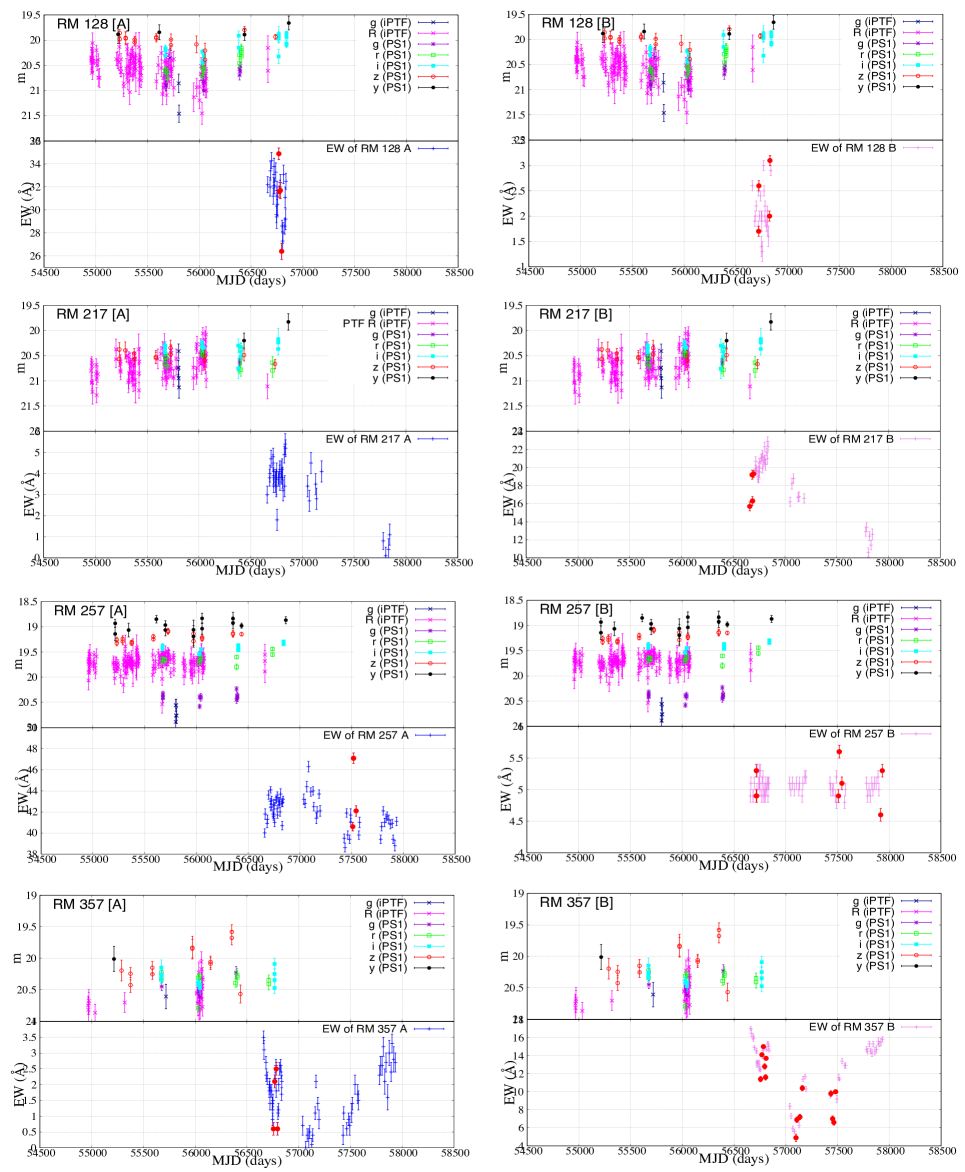
Figure 1: Light curves of the iPTF $g$ (navy), $R$ (magenta)-band, and the PS1 $g$ (purple), $r$ (green), $i$ (cyan), $z$ (red), and $y$ (black)-band ($top$), and EW variability of C IV BALs after dividing into A and B ($bottom$) for the class S1 quasars which show the significant BAL EW variability defined by H19. Red circles indicate data pairs that satisfy criteria of H19 for the significant short timescale BAL variability.

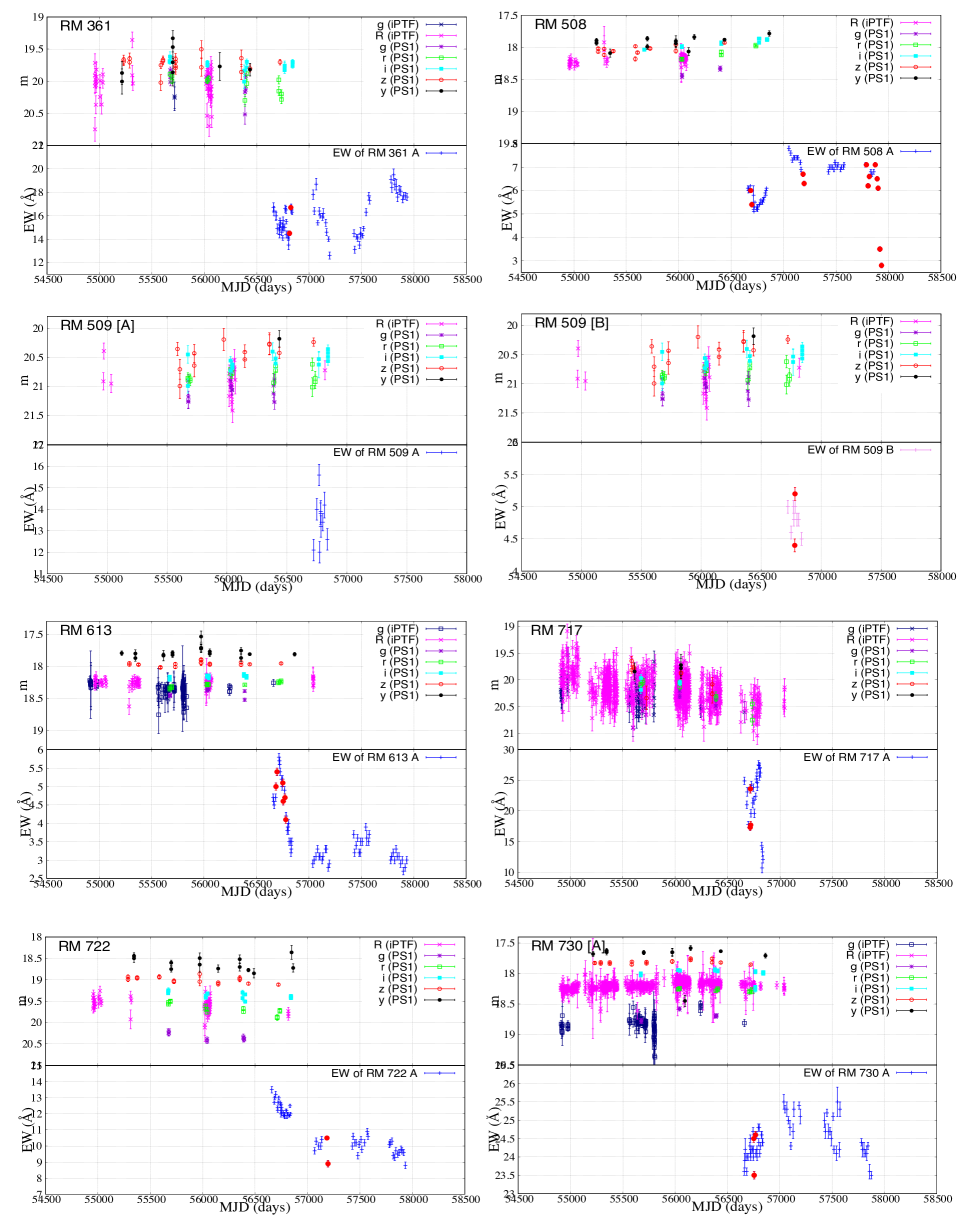
Figure 1: $Continued$.

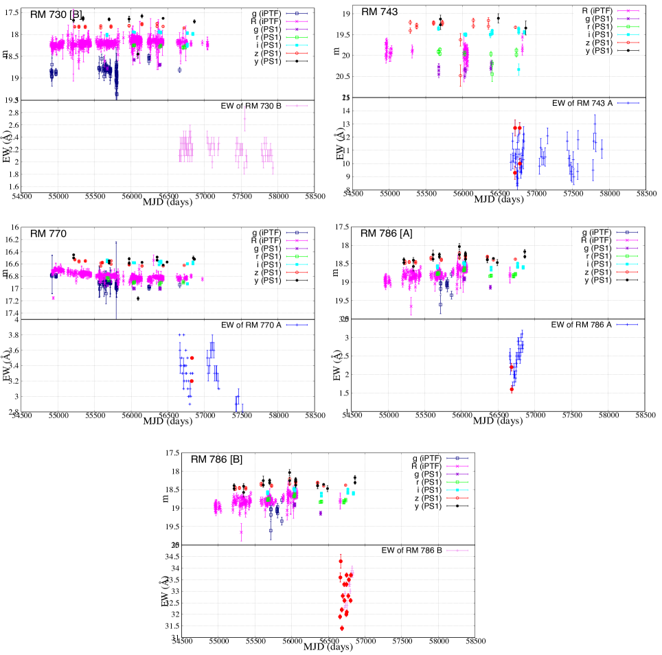
Figure 1: $Continued$.

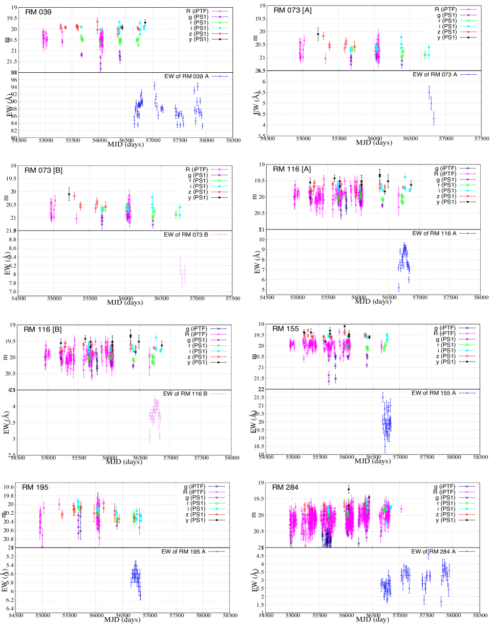
Figure 2: The same as Figure 1, but for the class S2 quasars.

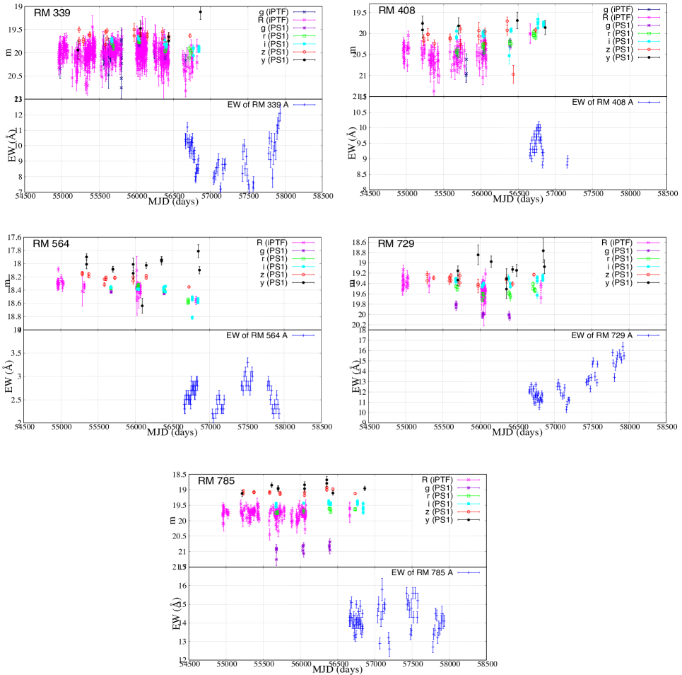
Figure 2: $Continued$.

Table 1: Physical properties of sample quasars

SDSS ID	RM ID	Redshift	$m_{i}$	$N_{\rm obs}$	Identifier	Class	log $\lambda L_{\lambda 1350}$	log $M_{\rm BH}$	$L_{\rm bol}/L_{\rm E}$
							(erg s-1)	($M_{\odot}$)
J141607.12+531904.8	RM 039	3.08	19.77	58	A	S2	45.619$\pm$0.003	8.48$\pm$0.07	0.109$\pm$0.017
J141741.72+530519.0	RM 073	3.43	20.37	3	A, B	S2	$\ldots$	$\ldots$	$\ldots$
J141432.46+523154.5	RM 116	1.88	19.68	64	A, B	S2	45.652$\pm$0.001	8.90$\pm$0.03	0.044$\pm$0.003
J141103.17+531551.3	RM 128	1.86	20.01	50	A∗, B∗	S1	45.359$\pm$0.002	8.68$\pm$0.05	0.037$\pm$0.004
J141123.68+532845.7	RM 155	1.65	19.65	41	A	S2	45.364$\pm$0.001	$\ldots$	$\ldots$
J141935.58+525710.7	RM 195	3.22	20.33	59	A	S2	$\ldots$	$\ldots$	$\ldots$
J141000.68+532156.1	RM 217	1.81	20.39	41	A, B∗	S1	45.382$\pm$0.002	8.67$\pm$0.02	0.040$\pm$0.001
J140931.90+532302.2	RM 257	2.43	19.54	65	A∗, B∗	S1	45.782$\pm$0.005	9.19$\pm$0.04	0.031$\pm$0.002
J141927.35+533727.7	RM 284	2.36	20.22	63	A	S2	45.642$\pm$0.001	9.05$\pm$0.05	0.031$\pm$0.003
J142014.84+533609.0	RM 339	2.01	20.00	64	A	S2	45.743$\pm$0.001	8.94$\pm$0.01	0.050$\pm$0.001
J141955.27+522741.1	RM 357	2.14	20.23	65	A∗, B∗	S1	$\ldots$	$\ldots$	$\ldots$
J142100.22+524342.3	RM 361	1.62	19.46	66	A∗	S1	45.576$\pm$0.001	$\ldots$	$\ldots$
J141409.85+520137.2	RM 408	1.74	19.63	65	A	S2	45.708$\pm$0.001	8.47$\pm$0.09	0.137$\pm$0.028
J142129.40+522752.0	RM 508	3.21	18.12	69	A∗	S1	46.919$\pm$1.000	10.35$\pm$1.00	0.029$\pm$0.095
J142233.74+525219.8	RM 509	2.65	20.30	10	A, B∗	S1	$\ldots$	$\ldots$	$\ldots$
J142306.05+531529.0	RM 564	2.46	18.24	67	A	S2	46.484$\pm$0.000	9.42$\pm$0.01	0.091$\pm$0.002
J141007.73+541203.4	RM 613	2.35	18.12	68	A∗	S1	46.591$\pm$0.001	9.10$\pm$0.01	0.245$\pm$0.005
J141648.26+542900.9	RM 717	2.17	19.69	49	A∗	S1	$\ldots$	$\ldots$	$\ldots$
J142419.18+531750.6	RM 722	2.54	19.49	59	A∗	S1	45.799$\pm$0.002	9.20$\pm$0.07	0.031$\pm$0.005
J142404.67+532949.3	RM 729	2.76	19.56	63	A	S2	46.074$\pm$0.001	9.10$\pm$0.01	0.074$\pm$0.001
J142225.03+535901.7	RM 730	2.69	17.98	65	A∗, B	S1	$\ldots$	$\ldots$	$\ldots$
J142405.10+533206.3	RM 743	1.74	19.18	49	A∗	S1	45.389$\pm$0.002	8.53$\pm$0.01	0.057$\pm$0.001
J142106.86+533745.2	RM 770	1.86	16.46	69	A∗	S1	46.948$\pm$0.003	9.31$\pm$0.10	0.344$\pm$0.007
J141322.43+523249.7	RM 785	3.72	19.19	67	A	S2	$\ldots$	$\ldots$	$\ldots$
J141421.53+522940.1	RM 786	2.04	18.63	68	A∗, B∗	S1	$\ldots$	$\ldots$	$\ldots$

3 Results

3.1 Correlation between UV flux and C IV BAL variability

As a first step to examine UV flux variability and BAL variability simultaneously, in Figures 1 and 2, we show light curves of the iPTF $g,R$ data and the PS1 $grizy$ data with BAL EWs ([A] and [B]) for the 34 BALs in the 25 quasars (i.e., excluding the data of RM 565 and RM 631) on the same time axis for the classes S1 and S2 quasars. In Figures 1 and 2, only 5 quasar/BAL pairs with the iPTF $R$-band photometric data satisfy the criteria in Section 2.2.1 (RM 284 [A], RM 339 [A], RM 717 [A], RM 730 [A], RM 730 [B], and RM770 [A]; hereafter, $five~{}quasars$). As a next step, we show the relation of the iPTF $R$-band variability $\Delta R$ versus the EW variability $\Delta EW$ (Figure 3). In Figure 4, we also indicate $\Delta R/\bigl{<}R\bigr{>}$ versus $\Delta EW/\bigl{<}EW\bigr{>}$ divided by $\Delta\tau$ for the $five~{}quasars$. We denote the details of these distributions for the $five~{}quasars$ in the following sections, including their spectral features (see also APPENDIX A in H19). The redshift, i-band magnitudes, and the class (S1 or S2) of each quasar and BAL are summarized in the parenthesis.

3.1.1 RM 284 [A] ($z=2.36,m_{i}=20.22,class:S2$)

In the RM284 spectrum, an extremely high velocity C IV trough is detected, and its velocity reaches from $\sim$ 35,000 to $\sim$ 59,000 km s^-1, that makes detection of any Si IV absorption in BAL[A] unclear. Al III absorption also does not clearly appear on the spectrum.

In Figure 3a, the number of data pair $N$ for $R$-band light curve data points and C IV BAL EWs is 17 (136 combinations of the observation epochs), which is the largest numbers in the $five~{}quasars$. We cannot find correlation of the distribution ($r=-0.03$, $r_{\Delta\tau<5}=0.04$). In Figure 4a, the distribution shows a weak or a moderate correlation ($r=0.39$, $r_{\Delta\tau<5}=0.42$ with $p$-values$<$0.04).

3.1.2 RM 339 [A] ($z=2.01,m_{i}=20.00,class:S2$)

This quasar’s spectrum contains Si IV and Al III BALs, whose velocity shifts are similar to the C IV trough. Figures 3b and 4b exhibit no possible correlations of the distributions in any timescales (i.e., $|r|<0.3$ or $p$-values$>$0.05).

3.1.3 RM 717 [A] ($z=2.17,m_{i}=19.69,class:S1$)

The C IV BAL of this quasar (BAL[A]) is composed of multiple components, and the accompanying Si IV BAL also exhibits a similar structure. BAL[A] showed the largest EW variability amplitude in the $five~{}quasars$. In Figure 3c, the $\Delta R$ - $\Delta EW$ distribution is shown no correlations ($r=-0.01$, $r_{\Delta\tau<5}=-0.07$). In Figure 4c, the correlation coefficient for all of data points indicates a weak correlation ($r=0.34$ with a $p$-value$<$0.01).

3.1.4 RM 730 [A], [B] ($z=2.69,m_{i}=17.98,class:S1$)

The spectrum of RM 730 contains two C IV BALs (BAL[A] and BAL[B]) separated by $\sim$ 500 km s^-1 from a red edge of the BAL[A] to a blue edge of the BAL[B], Only the BAL[A] exhibits a short timescale (rapid) variability based on criteria as defined in H19. A Si IV BAL and shallow Al III features (not BAL) are detected at velocities corresponding to BAL[A]. There are no BAL features of Si IV , Al III  , or P V at velocities associated to BAL[B].

The quasar does not show significant flux variability (i.e., $\Delta R<3\sigma$ photometric error). Figure 3d (for RM 730 [A]) presents EW variability ($\Delta EW$) that are comparable to these of RM 284 [A] and RM 339 [A], and Figure 3e (for RM 730 [B]) shows smaller EW variability than those of RM 284 [A], RM 339 [A], RM 717 [A], and RM 730 [A]. In Figures 3d, 3e, and 4d, there are no possible correlations in the $\Delta R$ — $\Delta EW$ distributions ($r=0.006$, $r_{\Delta\tau<5}=0.17$ for Figure 3d, $r=0.18$, $r_{\Delta\tau<5}=0.31$ with $p$-value=0.25 for Figure 3e, and $r=-0.06$, $r_{\Delta\tau<5}=-0.11$ for Figure 4d). Meanwhile, Figure 4e exhibits a strong correlation ($r=0.88$, $r_{\Delta\tau<5}=0.90$ with $p$-values$<$0.0001 for RM 730 [B]).

3.1.5 RM 770 [A] ($z=1.86,m_{i}=16.46,class:S1$)

This quasar is the apparently brightest in the H19 sample and does not contain both Si IV and Al III absorptions. The quasar also shows no significant flux variability within $R$-band photometric errors. In Figures 3f and 4f, we find no possible correlations of the distributions with $|r|<0.3$ or $p$-values$>$0.11.

In Figure 4, three of six distributions (i.e., except for RM 339 [A], RM 730 [A], and RM 770 [A]) present weak, moderate, or the strong correlation, and we also find that the correlation coefficients $r$ and $r_{\Delta\tau<5}$ are comparable for each BAL of the $five~{}quasars$.

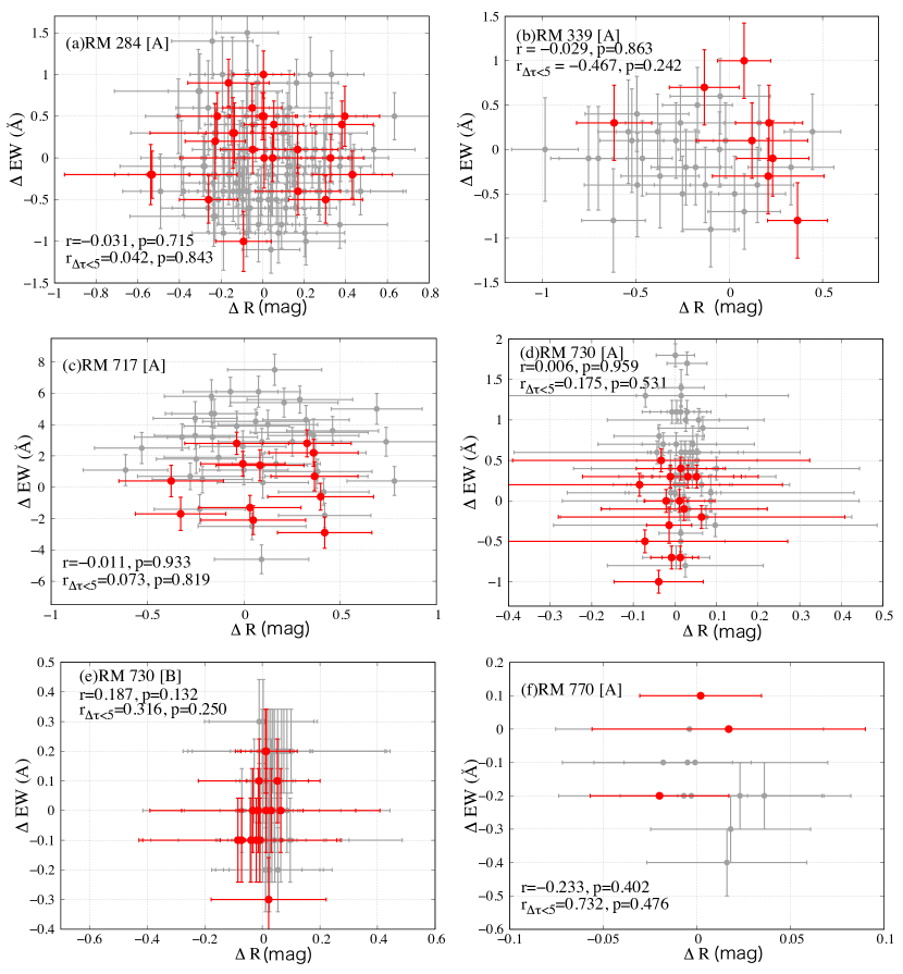
Figure 3: Distributions of $\Delta R$ versus $\Delta EW$ for (a) RM 284 [A], (b) RM 339 [A], (c) RM 717 [A], (d) RM 730 [A], (e) RM 730 [B], and (f) RM 770 [A]. Filled gray and red circles indicate the data points whose time separation is larger and smaller than 5 days. The correlation coefficients $r$ (for all of data points) and $r_{\Delta\tau<5}$ (for data point of $\Delta\tau<$ 5 days) with the associated $p$-values are described in each panel.

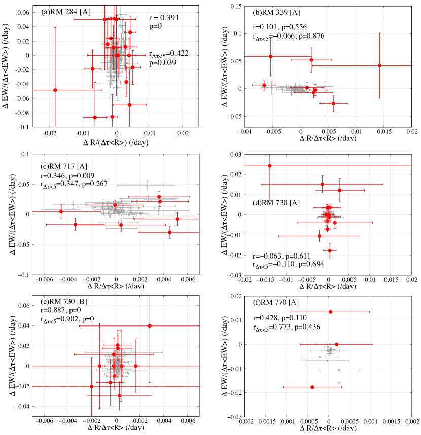
Figure 4: The same as Figure 3, but for distributions of $\Delta R/\bigl{<}R\bigr{>}$ versus $\Delta EW/\bigl{<}EW\bigr{>}$ both of which are divided by the rest-frame time separations $\Delta\tau$. The $p$-values with zero values indicate $p$-value$<$0.0001.

3.2 Structure Function Analysis

The PS1 DR2 data enable detailed structure function analysis to compare between the classes S1 and S2 quasars. On the other hand, it is difficult to investigate structure function analysis based on eqn. (3) using the iPTF $g,R$-band data due to large photometric error, since the average values of photometric error $\bigl{<}\sigma_{ij}^{2}\bigr{>}$ excess the mean UV flux variability amplitudes $\bigl{<}|\Delta m(\Delta\tau)|\bigr{>}^{2}$ especially in short timescale.

The rest-frame wavelength range through photometric bands depends on the redshifts of individual quasars. Therefore, we calculate structure functions for four bins of the rest-frame wavelength with the red-edges of the PS1 $grizy$ bands at the following rest-frame wavelength ($\lambda_{\rm red}$); (a) $\lambda_{\rm red}<2000~{}{\rm\AA}$, (b) $2000~{}{\rm\AA}<\lambda_{\rm red}<2500~{}{\rm\AA}$, (c) $2500~{}{\rm\AA}<\lambda_{\rm red}<3000~{}{\rm\AA}$, and (d) $\lambda_{\rm red}>3000~{}{\rm\AA}$, corresponding to full wavelength ranges ($\lambda_{\rm blue}<\lambda<\lambda_{\rm red}$; $\lambda_{\rm blue}$ corresponds to blue-edges of the following full wavelength ranges) of (a) $877~{}{\rm\AA}<\lambda<1991~{}{\rm\AA}$, (b) $1510~{}{\rm\AA}<\lambda<2498~{}{\rm\AA}$, (c) $2007~{}{\rm\AA}<\lambda<2989~{}{\rm\AA}$, and (d) $2603~{}{\rm\AA}<\lambda<3820~{}{\rm\AA}$ for the all of photometric data of the 25 quasars, respectively.

We estimate the structure function for the classes S1 and S2 quasars, including the short timescale variability $SF(\Delta\tau<10$ day). In the characterization of structure functions, power-law (e.g., Hook et al., 1994; Enya et al., 2002; Vanden Berk et al., 2004; MacLeod et al., 2012),

$$SF(\Delta\tau)=\Biggl{(}\frac{\Delta\tau}{\Delta\tau_{p}}\Biggr{)}^{\gamma}\equiv b\Delta\tau^{\gamma},$$ (6)

or a damped random walk (DRW: e.g., Kelly et al., 2009; MacLeod et al., 2010, 2012; Kozłowski, 2016a; Graham et al., 2017),

$$SF(\Delta\tau)=SF_{\infty}\sqrt{1-{\rm exp}(-\Delta\tau/\Delta\tau_{\rm DRW})},$$ (7)

is usually employed, where $\gamma$ and $\Delta\tau_{p}$ in eqn. (6) are the power-law index and the time scale such that $SF(\Delta\tau_{p})$ equals 1 mag. $SF_{\infty}$ and $\Delta\tau_{\rm DRW}$ in eqn. (7) are the asymptotic value at $\Delta\tau$ = $\infty$ and characteristic timescale, respectively. Figure 5 shows the structure functions of the light curves with fitted lines and describing fitted parameters of eqns. (6) and (7). Due to the large uncertainty in fitted parameters, we cannot evaluate accurate values for $\Delta\tau_{p}$ and $\Delta\tau_{\rm DRW}$; fitting errors of these two parameters exceed their own values.

Besides the analysis above for the continuum variability, we also apply the same approach to the structure function analysis for C IV EW variability based on eqns. (4) and (5) to these fitting models (Figure 6). In Figure 6b, we introduce another category to the classes S1 and S2 quasars; C IV BALs with significant short timescale variability defined by H19 are marked in asterisks in Table 1 ($*$) or not ($None$). In this category, we cannot make a quantitative physical parameter $\Delta\tau_{p}$ with the large uncertainty. As a similar BAL variability trend to the classes S1 and S2 quasars, the category $*$ shows the systematically larger BAL variability than that of the category “None”. The overall trends is that there is no clear difference in UV flux variability amplitudes between S1 and S2 (Figure 5), while BAL variability of the class S1 quasars (or “$*$”) are systematically larger than that of the class S2 (or “None”) from short to long timescales (Figure 6).

The flux we monitored in this study has larger wavelength than those of ionizing EUV flux. Therefore, we test flux variability dependence on the rest-frame wavelength to clarify a relation between the UV and ionizing continuum to C IV  ions ($h\nu>~{}$47 eV, $\lambda<260{\rm\AA}$). In general, the shorter the wavelength is, the larger quasar variability becomes (i.e., bluer-when-brighter (BWB) trend; e.g., Giveon et al., 1999; Vanden Berk et al., 2004; Kokubo et al., 2014). Then we characterize the trend for the class S2 quasars by

$$SF(\lambda)=a_{0}\exp{(-\lambda/\lambda_{0})},$$ (8)

where $a_{0}$ and $\lambda_{0}$ are fitting parameters (Vanden Berk et al., 2004). In Figure 7, the class S2 quasars show a weak BWB trend in contrast to the class S1 quasars with large photometric errors.

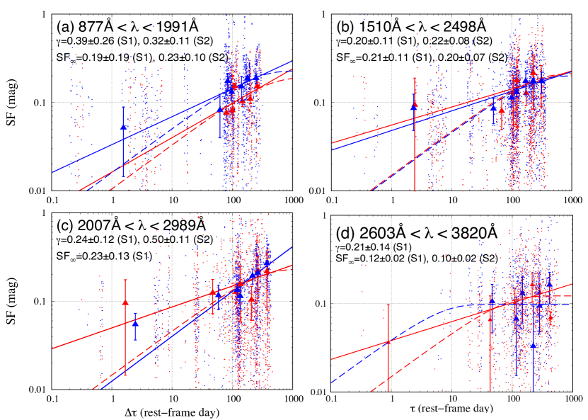
Figure 5: Structure Functions for photometric data of the class S1 (red triangle) and S2 (blue triangle) quasars, by dividing the rest-frame wavelength into 4 ranges; (a) $877~{}{\rm\AA}<\lambda<1991~{}{\rm\AA}$, (b) $1510~{}{\rm\AA}<\lambda<2498~{}{\rm\AA}$, (c) $2007~{}{\rm\AA}<\lambda<2989~{}{\rm\AA}$, and (d) $2603~{}{\rm\AA}<\lambda<3820~{}{\rm\AA}$. Red and blue dots represent the flux variability of 25 sample for all combinations of the observation epochs, corresponding to the classes S1 and S2 quasars. The structure functions of the classes S1 (red lines) and S2 (blue lines) quasars are fitted with a power low ($solid~{}line$) and a DRW ($dashed~{}line$). On short timescale ($<~{}$10 days), the structure function of the class S1 (or S2) quasars in panels (a) (or (d)) cannot be obtained due to larger photometric error than their mean flux variability. Fitting parameters of eqns. (6) and (7) are described in each panel.

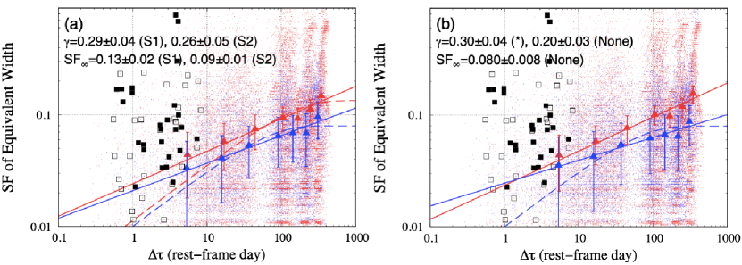
Figure 6: The same as Figure 5, but for the structure functions of C IV BAL EWs; (a) for the classes S1 and S2 quasars, including both BAL[A] and BAL[B], (b) for the C IV BALs that presented short timescale variability marked with asterisks in Table 1 ($*$: red) or not (None: blue). Red and blue dots indicate the UDSFs of 25 sample with smaller uncertainties ($\sigma_{\rm UDSF}<0.1$), corresponding to the classes S1 and S2 quasars. Filled (or open) black squares indicate short timescale significant variability of BAL[A] (or BAL[B]) defined by H19, and these plots are represented as UDSFs.

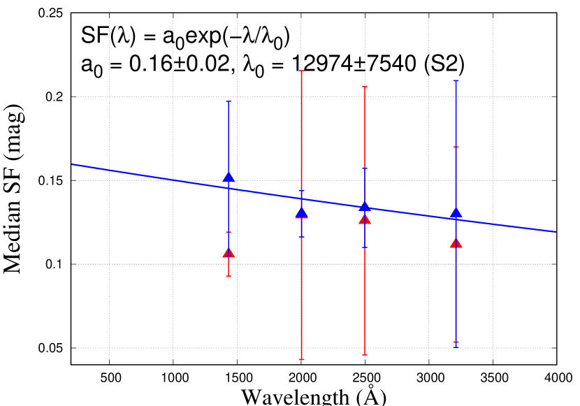
Figure 7: The median structure functions as a function of the rest-frame wavelength for the class S1 (red triangle) and S2 (blue triangle) quasars. The structure functions are the median values of each panel of Figure 5. The class S2 quasars are well fitted by eqn. (8). The fitting parameters are also shown.

3.3 Correlation between C IV BAL EW variability and Physical Properties of Sample Quasars

In order to probe the relation between BAL variability and physical properties of quasars, we also analysis the correlation between structure functions of C IV BAL EWs and physical parameters of the quasars such as bolometric luminosities $L_{\rm bol}$, black hole masses $M_{\rm BH}$, and Eddington ratios $L_{\rm bol}/L_{\rm Edd}$ after dividing into the classes S1 and S2 quasars. As listed in Table 1, we obtain these physical parameters from Grier et al. (2019) for 17 (bolometric luminosities), 15 (black hole masses) and 15 (Eddington ratios) out of the 25 quasars. Since the BAL variability is supposed to be sensitive to the ionization flux, we also study the relation between BAL variability and a physical quantity proportional to accretion disk temperature at an inner radius $T_{\rm in}~{}(\propto L_{\nu}^{3/8}M_{\rm BH}^{-3/4}\propto L_{\rm bol}^{3/8}M_{\rm BH}^{-3/4};$ see Section 4.1.3 and 4.2). For the 25 quasars, we assume the typical SED described by the bolometric corrections for $L_{\rm bol}=\zeta\lambda L_{\lambda}$, where $L_{\lambda}$ is a monochromatic luminosity, and factors $\zeta$ are 4.2, 5.2, and 8.1 for 1450, 3000, and 5100 ${\rm\AA}$, respectively (Runnoe et al., 2012a).

Figure 8 summarizes the relations between BAL variability in each timescale and physical parameters. In relation to Figure 8, Table 2 lists the correlation coefficients with their $p$-values for each rest-frame time separation range (unit of days): $\Delta\tau<$ 10, $10<\Delta\tau<$ 30, $30<\Delta\tau<$ 100, and $100<\Delta\tau$. Based on Table 2, we denote the details of the correlation between BAL variability and physical parameters in the following sections.

3.3.1 $SF_{\rm BAL}$ vs. $L_{\rm bol}$: Figure 8a

The classes S1 and S2 quasars do not show possible correlations ($0.3<|r|$ or $0.3<|r|<0.4$ with $p$-value$>$0.05) for any time separations.

3.3.2 $SF_{\rm BAL}$ vs. $M_{\rm BH}$: Figure 8b

Throughout, the class S1 quasars do not indicate possible correlations. On the other hand, the class S2 quasars show a moderate positive ($r=0.47$ with $p$-value $=$ 0.03) or a strong positive correlation ($r=0.67$ with $p$-value $=$ 0.02) after $\Delta\tau>30$ days.

3.3.3 $SF_{\rm BAL}$ vs. $L_{\rm bol}/L_{\rm Edd}$: Figure 8c

As a whole, the class S2 quasars present strong negative correlations ($r<-0.6$ with $p$-value $<$ 0.03). In contrast, the class S1 quasars show no correlations in any cases.

3.3.4 $SF_{\rm BAL}$ vs. $L_{\rm bol}^{3/8}M_{\rm BH}^{-3/4}$: Figure 8d

The class S2 quasars show strong negative correlations for $\Delta\tau>$ 10 days, while the class S1 quasars do not exhibit possible correlations.

There are no possible correlations between BAL variability and physical parameters for the class S1 quasars, and the overall distribution of the class S1 (14 quasars) and S2 (11 quasars) quasars ($|r_{\rm All}|<0.3$). Here, we emphasize that RM 613 and RM 770 whose Eddington ratios are comparably higher in the class S1 quasars ($L_{\rm bol}/L_{\rm Edd}=0.245\pm 0.005$, and $0.344\pm 0.007$, respectively) exhibit a different trend from the class S2 quasars with the strong negative correlation between C IV BAL variability and Eddington ratios (for $L_{\rm bol}/L_{\rm Edd}<$ 0.2).

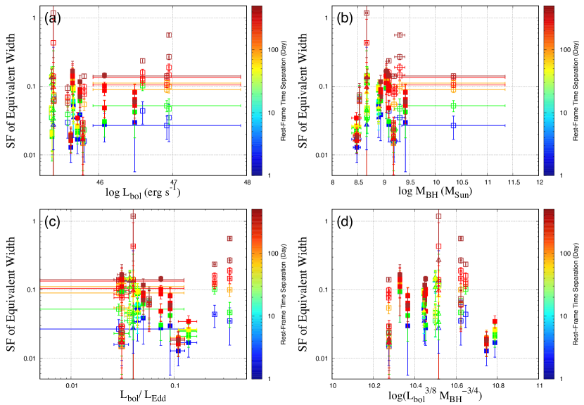
Figure 8: The relation between structure functions of C IV BAL EWs and physical properties at each rest-frame time-lag. Each panels indicate structure functions of BAL[A][B] for individual quasars based on eqn. (4) versus (a) bolometric luminosity, (b) black hole mass, (c) Eddington ratio, and (d) temperature of the accretion disk based on the standard model. Open and filled squares (or triangles) show the distribution for BAL[A] (or BAL[B]) of the classes S1 and S2 quasars. Colors indicate rest-frame time separation, where redder colors correspond to larger time lag, as shown in the color keys.

Table 2: The correlation coefficient with $p$-values between BAL variability and physical parameters

The range of time separation $\Delta\tau$ (days)	$r_{\rm S1}$a ($p$-values): 14 quasars	$r_{\rm S2}$b ($p$-values): 11 quasars	$r_{\rm All}$c ($p$-values): 25 quasars
$SF_{\rm BAL}$ vs. $L_{\rm bol}$ (Figure 8a)
$\Delta\tau<$ 10	-0.373 (0.231)	-0.083 (0.831)	-0.297 (0.190)
$10<\Delta\tau<$ 30	-0.202 (0.392)	0.135 (0.569)	-0.122 (0.452)
$30<\Delta\tau<$ 100	0.203 (0.467)	0.322 (0.283)	0.255 (0.189)
$100<\Delta\tau$	0.060 (0.722)	-0.051 (0.825)	0.062 (0.646)
For all data of $\Delta\tau$	0.064 (0.560)	0.163 (0.203)	0.088 (0.291)
$SF_{\rm BAL}$ vs. $M_{\rm BH}$ (Figure 8b)
$\Delta\tau<$ 10	-0.481 (0.134)	0.382 (0.349)	-0.268 (0.266)
$10<\Delta\tau<$ 30	-0.320 (0.182)	0.461 (0.072)	-0.118 (0.497)
$30<\Delta\tau<$ 100	0.039 (0.894)	0.671 (0.023)	0.228 (0.271)
$100<\Delta\tau$	-0.142 (0.429)	0.475 (0.029)	-0.044 (0.753)
For all data of $\Delta\tau$	-0.080 (0.489)	0.495 (0)	0.010 (0.909)
$SF_{\rm BAL}$ vs. $L_{\rm bol}/L_{\rm Edd}$ (Figure 8c)
$\Delta\tau<$ 10	-0.098 (0.774)	-0.765 (0.026)	-0.167 (0.493)
$10<\Delta\tau<$ 30	0.005 (0.984)	-0.754 (0)	-0.144 (0.407)
$30<\Delta\tau<$ 100	0.267 (0.355)	-0.737 (0.009)	0.062 (0.769)
$100<\Delta\tau$	0.208 (0.244)	-0.825 (0)	0.197 (0.153)
For all data of $\Delta\tau$	0.187 (0.103)	-0.670 (0)	0.146 (0.093)
$SF_{\rm BAL}$ vs. $L_{\rm bol}^{3/8}M_{\rm BH}^{-3/4}$ (Figure 8d)
$\Delta\tau<$ 10	0.377 (0.253)	-0.687 (0.059)	0.093 (0.705)
$10<\Delta\tau<$ 30	0.326 (0.173)	-0.687 (0.003)	-0.025 (0.886)
$30<\Delta\tau<$ 100	0.112 (0.703)	-0.817 (0.002)	-0.207 (0.320)
$100<\Delta\tau$	0.241 (0.177)	-0.751 (0)	0.107 (0.443)
For all data of $\Delta\tau$	0.181 (0.115)	-0.688 (0)	0.036 (0.677)

Note. — The correlations with $|r|>0.3$ and $p$-value$<$0.05 are marked in bold face. The $p$-values with zero values indicate $p$-value$<$0.0001.

4 Discussion

4.1 Ionization state change in Outflows

We first consider whether a change in the ionization condition of outflow winds explains the observational results.

4.1.1 Correlation between the BAL EWs and quasar variability

Trévese et al. (2013) found a clear correlation between variability of C IV BAL EWs and the rest-frame UV flux variability in a gravitational lensed BAL quasar APM 08279+5255, supporting the ionization state change as a possible origin of the BAL variability. Vivek (2019) also found 78 quasars of the SDSS DR12 with high signal-to-noise ratio spectra show a weak/moderate correlation between BAL and flux variability taken by the SDSS and the Catalina Real-Time Transient Survey (CRTS) catalog. He et al. (2017) analyzed the multi-epoch SDSS DR12 spectra of BAL quasars, and using EW ratios ($R$) of Si IV to C IV BAL, they suggested that a recombination timescale of BAL clouds is only a few days. This means the typical absorber density $n_{e}$ is $\sim 10^{6}$ cm^-3. Lu & Lin (2019) discovered a clear correlation between BAL variability and flux changes for 21 BAL quasars from the SDSS-I/II/III, including some of our sample (RM 357, RM 722, RM 729, RM 730, and RM 786). These studies conclude that changes in ionizing continuum cause BAL variability in a various time scale.

Most of distributions in Figure 3 show no positive or negative correlations. Meanwhile, BAL EW variability in Figure 4 shows weak, moderate positive ($r=0.39$ and $r_{\Delta\tau<5}=0.42$ for RM 284 [A], and $r=0.34$ for RM 717 [A]) or a strong positive ($r>0.7$ for RM 730 [B]) correlation with $R$-band variability in the timescale from $<$10 days to longer; these C IV BAL EWs increase (or decrease) when these quasars dim (or brighten) in short timescales. This result suggests a recombination time of outflow gas clouds is within a few days or a week. In contrast to the preceding argument, RM 339 [A], RM 730 [A], RM 770[A] do not indicate short timescale BAL variability. Moreover, relatively bright quasars RM 730 ($m_{i}=17.98$) and RM 770 ($m_{i}=16.46$ and log$L_{bol}=46.948\pm 0.003$) show no significant $R$-band variability (Figure 1). This trend likely follows a negative correlation between variability amplitude and the quasar luminosity (e.g, Giveon et al., 1999; Vanden Berk et al., 2004; MacLeod et al., 2012). Thus, we speculate BAL variability is mainly caused by quasar flux variability. Especially, less luminous quasars tend to show the correlation between BAL and flux variability. In terms of RM 339 [A], RM 730 [A], and RM 770 [A], it is necessary to consider another mechanism to change BAL EWs (see Section 4.2).

4.1.2 Structure Function

The structure functions in Figure 5 show following trends; (i) variability amplitudes become slightly larger with time separations as suggested in previous studies (e.g., Vanden Berk et al., 2004; MacLeod et al., 2010), and power-law indexes $\gamma$ in each panel are consistent with those of Vanden Berk et al. (2004), (ii) DRW model is not well fitted at short-timescale, as already reported by MacLeod et al. (2012). In other words, the classes S1 and S2 quasars in this study have consistent properties of flux variability with samples in previous studies.

Based on the ionization state change scenario in outflows, the larger flux changes in quasar yield, the larger EW variability in BALs. According to the scenario, the class S1 quasars, with larger BAL variability amplitudes than the class S2 quasars (Figures 6a and 6b), would show relatively larger flux variability than the class S2 quasars. However, contrary to this expectation, Figure 5 indicates almost comparable flux variability amplitudes with the classes S1 and S2 quasars in each panel.

In Figures 6a and 6b, we conjecture another possibility for the systematic difference in the BAL variability trend between the class S1 and S2 quasars (or the categories “$*$” and “None”); the BAL variability follows the trend that absorption lines with shallower line profiles (smaller EWs) more easily show the larger fractional variability $|\Delta EW/\bigl{<}EW\bigr{>}|$ (e.g, Lundgren et al., 2007). However, there is no significant difference in $\bigl{<}EW\bigr{>}$ between the class S1 (15.1 $\pm$ 0.4 ${\rm\AA}$) and S2 quasars (16.2 $\pm$ 0.3 ${\rm\AA}$) . Namely, the difference of their average EW ($\bigl{<}EW\bigr{>}$), which could cause BAL variability easily due to the ionization state change, can not be the origin behind the difference between the classes S1 and S2 quasars. Furthermore, in Figures 6a and 6b, significant BAL variability ($<$10-day) for BAL[A] show weak negative correlation between rest-frame time lag and $UDSF(<0.2)$ with a correlation coefficient of $r=-0.38$. The trend also suggests that BAL variability requires another physical process other than flux variability (see also Section 4.2).

4.1.3 Relation between BAL Variability and Physical Properties

In general, flux variability amplitude decreases with quasar luminosities, increases with black hole masses and decreases with Eddington ratios as already suggested in previous studies (e.g., Wold et al., 2007; Wilhite et al., 2008; Meusinger & Weiss, 2013; Rumbaugh et al., 2018) as explained in Section 4.1.1. If BAL variability is mainly driven by flux changes, the variability timescales and/or amplitude would also depend on physical properties of quasars.

We also evaluate the relation between BAL variability and the accretion disk temperature at an inner radius $T_{\rm in}$. Based on the standard thin accretion disk model (Shakura & Sunyaev, 1973), the effective temperature $T_{\rm eff}$ is proportional to $(M_{\rm BH}\dot{M}/R^{3})^{1/4}$, where $\dot{M}$ and $R$ are mass accretion rate and disk radius, respectively. For example, at the region of inner radius $R=3R_{\rm S}$ (Schwarzschild radius $R_{\rm S}=2GM_{\rm BH}/c^{2}\propto M_{\rm BH}$), the disk temperature $T_{\rm in}$ is proportional to $(\dot{M}/M_{\rm BH}^{2})^{1/4}$. The disk luminosity at optical/UV $L(=\nu L_{\nu})$, $\dot{M}$ and $M_{\rm BH}$ are related with $L\propto(\dot{M}M_{\rm BH})^{2/3}$ (i.e., $\dot{M}\propto L^{3/2}/M_{\rm BH}$; Collin & Kawaguchi, 2004). Therefore, the disk temperature $T_{\rm in}$ is described by

$$T_{\rm in}\propto L^{3/8}M_{\rm BH}^{-3/4}\propto L_{\rm bol}^{3/8}M_{\rm BH}^{-3/4}.$$ (9)

The negative correlation between BAL variability and the disk temperature $T_{\rm in}$ would also be expected, since, as well as the Eddington ratio ($\propto L_{\rm bol}M_{\rm BH}^{-1}$), the $T_{\rm in}$ is associated with bolometric luminosity and black hole mass. In fact, the class S2 quasars only show the strong correlation between structure functions of C IV BAL and physical properties of the Eddington ratio and $L_{\rm bol}^{3/8}M_{\rm BH}^{-3/4}$ (negative correlation) in Figure 8. These BAL variability trends are consistent with the relation between flux variability and physical parameters of quasars. The results also support the ionization state change scenario and are contrary to the cloud crossing scenario.

As described in Section 3.3, two quasars at higher Eddington ratios (the class S1 quasars RM 613 and RM 770) exhibit relatively large C IV BAL variability. The average C IV BAL EWs of these two quasars are smaller (4.8 $\pm$ 0.2 ${\rm\AA}$ for RM 613, and 3.6 $\pm$ 0.1 ${\rm\AA}$ for RM 770) than those of the other quasars (15.1 $\pm$ 0.4 ${\rm\AA}$ as the average EW of the class S1 quasars). The C IV BAL variability trend of RM 613 and RM 770 suggests the observational trend that shallower intrinsic absorption lines more easily show larger BAL variability as explained in Section 4.1.2. On the other hand, at lower Eddington ratios ($L_{\rm bol}/L_{\rm Edd}<0.1$), the class S1 quasar RM 217 ($\bigl{<}EW\bigr{>}=$ 4.2 $\pm$ 0.4 ${\rm\AA}$ for BAL[A]) presents the largest BAL variability, while RM 257 [A] with a relatively large average EW ($\bigl{<}EW\bigr{>}=$ 42.6 $\pm$ 0.4  ${\rm\AA}$) exhibits the smallest BAL variability in the class S1 quasars. As a whole, the class S1 quasars have a larger sample variance of the average C IV BAL EW than that of the class S2 quasars except for the data of RM 039 with $\bigl{<}EW\bigr{>}$ of 88.5 $\pm$ 0.7 ${\rm\AA}$ (see APPENDIX A and Figure A in this paper). Consequently, the variance of the average EW in the class S1 quasars yields no correlations in Figure 8.

In comparable EW of BAL samples, the correlation between BAL variability and black hole masses (positive correlation), and Eddington ratios or accretion disk temperature (negative correlation) indicates that the BAL variability amplitude depends on the properties of the accretion disk. Quasars with lower Eddington ratios frequently change the accretion rates (i.e., unstable fuel supply onto accretion disk). The frequent change of accretion rate causes rapid and large flux variability of quasars (c.f., Wilhite et al., 2008; Rumbaugh et al., 2018). Consequently, the ionization states in outflow winds can be affected by flux variability in quasars with lower Eddington ratios because of a sudden increasing or decreasing of a fuel supply onto the accretion disk.

4.2 The Changes in Shielding Gas?

We find several important results; (1) Among the $five~{}quasars$, three quasars present weak, moderate, or a strong positive correlation between the iPTF $R$-band variability and BAL variability (Figure 4), (2) there is almost no significant difference of flux variability amplitudes between BAL quasars with the significant EW variability and the others (Figure 5), while BAL variability for the class S1 are systematically larger than that for the class S2 from $<10$ days to longer timescales ($>10$ days) (Figure 6), and (3) BAL variability and physical parameters show a possible positive (black hole masses) and negative correlations (Eddington ratios and the accretion disk temperature) in the class S2 quasars (Figure 8). From Figure 6, the classes S1 and S2 quasars could show the systematic difference of flux variability between them based on the ionization state change. However, the result (2) does not show such a trend, and this fact indicates that the BAL variability cannot be explained only by the flux variability in quasars.

As an ancillary mechanism to explain short and/or long timescale BAL variability, the variations in shielding gas is proposed (c.f., Hamann et al., 2013); it is a inner disk flow that fails to escape from the disk (i.e., failed wind) and presents frequent variability in very short timescales of the order of days to weeks (Proga et al., 2000; Proga & Kallman, 2004; Proga et al., 2012; Giustini & Proga, 2019). The shielding gas appears to prevent over-ionization of outflows at a down stream. If the shielding gas locating at the innermost of an accretion disk fluctuates its own ionization state, an amount of ionizing photons (e.g, EUV continuum) is probably adjusted due to variations of the shielding gas. Consequently, outflows change their ionization state. As an observational suggestion, broad absorbing features via X-ray ultra-fast outflows have rapidly changed in a timescale of hours to months that is consistent with a typical timescale of the shielding gas (Saez et al., 2009; Gofford et al., 2014, see also Giustini & Proga 2019).

One of the candidate of shielding gas is a warm absorber that has been detected as absorption edges in X-ray spectra (e.g., Gallagher et al., 2002, 2006). Warm absorbers were originally proposed to avoid over-ionization of the outflows (Murray et al., 1995). In most case, strong X-ray warm absorbers are detected in spectra of BAL quasars. To put it another way, strong X-ray absorption is rarely detected in spectra of non-BAL quasars (e.g., HS 1700+6416; Lanzuisi et al., 2012). Notably, the result (2) indicates that the effect of variations in shielding gas is probably more prominent in the class S1 quasars, since the BAL variability timescales of this class are similar to that of the shielding gas (Proga et al., 2012). If we detect simultaneous changes of X-ray absorbers and BAL variability, the ionization state change scenario becomes more robust the physical mechanism of BAL variability.

5 Conclusion

We examined the correlation between the variability of flux for BAL quasars and their EWs in a various time scales from $<10$ days to a few years in the quasar rest-frame. In the study of the correlation, we used the data sets of EW of BALs taken by the Sloan Digital Sky Survey Reverberation Mapping (SDSS-RM) project, reported by H19 and photometric data taken by the iPTF) with $g$, $R$-band and the PS1 with $grizy$ bands. We divide the sample into two the classes (S1 and S2) according to the presence or the lack of short timescale BAL variability. Our results are summarized as follows.

• Among the $five~{}quasars$ that satisfy the conditions (1) and (2) in Section 2.2.1, three quasars present weak, moderate (for RM 284 and RM 717), and a strong correlation (for RM 730) between flux variability and BAL variability (Figure 4).

• The classes S1 and S2 quasars show no significant difference in flux variability amplitudes (Figure 5).

• There is systematic difference in BAL variability amplitudes between the classes S1 and S2 quasars (Figure 6).

• The distributions of BAL variability amplitudes and black hole masses, Eddington ratios and the accretion disk temperature exhibit strong negative correlations for the class S2 quasars (Figure 8).

These results indicate that BAL variability primarily requires variations in the ionizing continuum, and secondarily an ancillary mechanism such as variability in shielding gas except for the gas motion scenarios.

Appendix A Relation between BAL Variability, Eddington Ratio, and Average EW

We investigate the relation between BAL variability and Eddington ratio, and the average EW with following distributions: (i) Eddington ratio versus average EW, (ii) BAL variability versus Eddington ratio, and (iii) BAL variability versus average EW in Figure A. BALs of the class S1 quasars with comparably smaller average EW, RM 217, RM 613, and RM 770 (whose average EW are $\bigl{<}EW\bigr{>}=4.2\pm 0.4~{}{\rm\AA},4.8\pm 0.2~{}{\rm\AA}$, and $3.6\pm 0.1~{}{\rm\AA}$, respectively) exhibit extremely large BAL variability in the distributions (ii) and (iii). In contrast, those for RM 257 [A] with $\bigl{<}EW\bigr{>}=~{}$42.6 $\pm$ 0.4$~{}{\rm\AA}$ show the smallest BAL variability in the class S1 quasars. The sample variance of $\bigl{<}EW\bigr{>}$ for the class S1 quasar ($s^{2}=158.4$ ${\rm\AA}^{2}$) is larger than that for the class S2 quasars ($s^{2}=10.5$ ${\rm\AA}^{2}$) except for RM 039 with $\bigl{<}EW\bigr{>}$ of 88.5 $\pm$ 0.7 ${\rm\AA}$. As a result, the class S1 quasars seem to have no correlation ($r_{\rm S1}=$ 0.19 and -0.29 for the distributions (ii) and (iii)). In terms of the class S2 quasars, they indicate negative correlations in the distributions (ii) ($r_{\rm S2}=-0.67$) and (iii) ($r_{\rm S2}=-0.46$). Especially in the distribution (ii), despite comparable average EWs for RM 116 [A], RM 339 [A], RM 408 [A], and RM 729 [A] ($\bigl{<}EW\bigr{>}=8.2\pm 0.3~{}{\rm\AA},9.7\pm 0.3~{}{\rm\AA},9.8\pm 0.2~{}{\rm\AA}$, and $11.8\pm 0.3~{}{\rm\AA}$, respectively), they suggest a negative correlation between BAL variability and Eddington ratios. This result indicates that the Eddington ratio can be an index of BAL variability. The negative correlation between the average EWs and BAL variability (distribution (iii); $r=-0.46$ for the class S2 quasars) means the trend that shallower absorption lines show larger fractional variability (e.g, Lundgren et al., 2007).

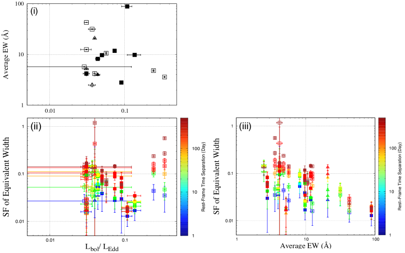
Figure A: The plot of Eddington ratios versus average EWs ($top$), Eddington ratios versus BAL variability (the same as Figure 8c; $bottom~{}left$), and average EWs versus BAL variability ($bottom~{}right$). The symbols (Open and filled squares or triangles) are the same in Figure 8. Colors for bottom panels indicate the rest-frame time separation, where redder colors correspond to larger time lag, as shown in the color keys.

References

- Barlow (1994) Barlow T. A. 1994, PASP, 106, 548
- Bertin & Arnouts (1996) Bertin, E., & Arnouts, S. 1996, \aas, 117, 393
- Blandford & Payne (1982) Blandford, R. D., & Payne, D. G. 1982, MNRAS, 199, 883
- Capellupo et al. (2011, 2012, 2013) Capellupo, D. M., Hamann, F., Shields, J. C., et al. 2011, MNRAS, 413, 908
- Capellupo et al. (2012) Capellupo, D. M., Hamann, F., Shields, J. C., Rodríguez Hidalgo, P., & Barlow, T. A. 2012, MNRAS, 422, 3249
- Capellupo et al. (2013) Capellupo, D. M., Hamann, F., Shields, J. C., Halpern, J. P., & Barlow, T. A. 2013, MNRAS, 429, 1872
- Chambers et al. (2016) Chambers, K. C., Magnier, E. A., Metcalfe, N., et al. 2016, ArXiv e-prints, arXiv:1612.05560
- Collin & Kawaguchi (2004) Collin S., & Kawaguchi T. 2004, A&A, 426, 797
- di Clemente et al. (1996) di Clemente, A., Giallongo, E., Natali, G., Trevese, D., & Vagnetti, F. 1996, ApJ, 463, 466
- Di Matteo et al. (2005) Di Matteo, T., Springel, V., & Hernquist, L. 2005, Nature, 433, 604
- Elvis (2012) Elvis M., 2012, in Chartas G., Hamann F., Leighly K. M., eds, Astronomical Society of the Pacific Conference Series Vol. 460, AGN Winds in Charleston. p. 186 (arXiv:1201.3520)
- Enya et al. (2002) Enya, K., Yoshii, Y., Kobayashi, Y., et al. 2002, ApJS, 141, 45
- Ferrarese & Merritt (2000) Ferrarese, L., & Merritt, D. 2000, ApJ, 539L, 9
- Filiz Ak et al. (2012) Filiz Ak, N., Brandt, W. N., Hall, P. B., et al. 2012, ApJ, 757, 114
- Filiz Ak et al. (2013) Filiz Ak, N., Brandt, W. N., Hall, P. B., et al. 2013, ApJ, 777, 168
- Flewelling et al. (2016) Flewelling H., Magnier, E. A., Chambers, K. C., et al., 2016, arXiv preprints, arXiv:1612.05243
- Gallagher et al. (2002) Gallagher, S. C., Brandt, W. N., Chartas, G., & Garmire, G. P. 2002, ApJ, 567, 37
- Gallagher et al. (2006) Gallagher, S. C., Brandt, W. N., Chartas, G., et al. 2006, ApJ, 644, 709
- Ganguly et al. (2001) Ganguly, R., Bond, N. A., Charlton, J. C., et al. 2001, ApJ, 549, 133
- Gibson et al. (2009a) Gibson, R. R., Brandt, W. N., Gallagher, S. C., & Schneider, D. P. 2009a, ApJ, 696, 924
- Gibson et al. (2008) Gibson, R. R., Brandt, W. N., Schneider, D. P., & Gallagher, S. C. 2008, ApJ, 675, 985
- Giustini & Proga (2019) Giustini, M., & Proga, D. 2019, A&A, 630, A94
- Giveon et al. (1999) Giveon, U., Maoz, D., Kaspi, S., Netzer, H., & Smith, P. S. 1999, MNRAS, 306, 637
- Gofford et al. (2014) Gofford, J., Reeves, J. N., Braito, V., et al. 2014, ApJ, 784, 77
- Graham et al. (2017) Graham, M. J., Djorgovski, S. G., Drake, A. J., et al. 2017, MNRAS, 470, 4112
- Grier et al. (2015) Grier, C. J., Hall, P. B., Brandt, W. N., et al. 2015, ApJ, 806, 111
- Grier et al. (2019) Grier, C. J., Shen, Y., Horne, K., et al. 2019, arXive-prints, arXiv:1904.03199
- Hamann et al. (2013) Hamann, F., Chartas, G., McGraw, S., et al. 2013, MNRAS, 435, 133
- Hamann et al. (2012) Hamann, F., Simon, L., Hidalgo, P. R., et al. 2012, ASP Conf. Ser. Vol. 460, AGN Winds in Charleston, San FranciscoAstron. Soc. Pac.pg. 47
- He et al. (2017) He, Z., Wang, T., Zhou, H., et al. 2017, ApJS, 229, 22
- Hemler et al. (2019) Hemler, Z. S., Grier, C. J., Brandt, W. N., et al. 2019 (H19), ApJ, 872, 21
- Hook et al. (1994) Hook, I. M., McMahon, R. G., Boyle, B. J., & Irwin, M. J. 1994, MNRAS, 268, 305
- Kelly et al. (2009) Kelly B. C., Bechtold J., & Siemiginowska A. 2009, ApJ, 698, 895
- Kokubo et al. (2014) Kokubo, M., Morokuma, T., Minezaki, T., Doi, M., Kawaguchi, T., Sameshima, H., & Koshida, S. 2014, ApJ, 783, 46
- Kozłowski (2016a) Kozłowski S. 2016a, ApJ, 826, 118
- Lanzuisi et al. (2012) Lanzuisi, G., Giustini, M., Cappi, M., et al. 2012, ApJ, 544, A2
- Law et al. (2009) Law N. M., Kulkarni S. R., Dekany R. G., et al. 2009, PASP, 121, 1395
- Lu & Lin (2019) Lu, W.-J., & Lin, Y.-R. 2019, arXive-prints, arXiv:1908.03844
- Lundgren et al. (2007) Lundgren, B. F., Wilhite, B. C., Brunner, R. J., et al. 2007, ApJ, 656, 73
- MacLeod et al. (2010) MacLeod, C. L., Ivezić, Ž., Kochanek, C. S., et al. 2010, ApJ, 721, 1014
- MacLeod et al. (2012) MacLeod, C. L., Ivezić, Ž., Sesar, B., et al. 2012, ApJ, 753, 106
- Meusinger & Weiss (2013) Meusinger, H., & Weiss, V. 2013, A&A, 560, A104
- Moll et al. (2007) Moll, R., et al. 2007, A&A, 463, 513
- Murray et al. (1995) Murray, N., Chiang, J., Grossman, S. A., Voit, G. M. 1995, ApJ, 451, 498
- Proga & Kallman (2004) Proga, D., & Kallman, T. R. 2004, ApJ, 616, 688
- Proga et al. (2012) Proga, D., Rodriguez-Hidalgo, P., & Hamann, F. 2012, AGN Winds in Charleston, 171
- Proga et al. (2000) Proga, D., Stone, J. M., & Kallman, T. R. 2000, ApJ, 543, 686
- Rau et al. (2009) Rau, A., Kulkarni, S. R., Law, N. M., et al. 2009, PASP, 121, 1334
- Rumbaugh et al. (2018) Rumbaugh, N., Shen, Y., Morganson, E., et al. 2018, ApJ, 854, 160
- Runnoe et al. (2012a) Runnoe, J. C., Brotherton, M. S., & Shang, Z. 2012a, MNRAS, 422, 478
- Saez et al. (2009) Saez, C., Chartas, G., & Brandt, W. N. 2009, ApJ, 697, 194
- Shakura & Sunyaev (1973) Shakura N. I., & Sunyaev R. A. 1973, A&A, 24, 337
- Shen et al. (2015) Shen, Y., Brandt, W. N., Dawson, K. S., et al. 2015, ApJS, 216, 4
- Tonry et al. (2012) Tonry, J. L., Stubbs, C. W., Lykke, K. R., et al. 2012, ApJ, 750, 99
- Trévese et al. (2007) Trévese, D., Paris, D., Stirpe, G. M., Vagnetti, F., & Zitelli, V. 2007, A&A, 470, 49
- Trévese et al. (2013) Trévese, D., Saturni, F. G., Vagnetti, F., et al. 2013, A&A, 557, A91
- Vanden Berk et al. (2004) Vanden Berk, D. E., Wilhite, B. C., Kron, R. G., et al. 2004, ApJ, 601, 692
- Vivek (2019) Vivek, M. 2019, MNRAS, 486, 2379
- Vivek et al. (2016) Vivek M., Srianand R., & Gupta N. 2016, MNRAS, 455, 136
- Vivek et al. (2012) Vivek M., Srianand R., Mahabal A., & Kuriakose V. C. 2012, MNRAS, 421, L107
- Wang et al. (2015) Wang, T., Yang, C., Wang, H., & Ferland, G. 2015, ApJ, 814, 150
- Weymann et al. (1991) Weymann, R. J., Morris, S. L., Foltz, C. B., & Hewett, P. C. 1991, ApJ, 373, 23
- Wilhite et al. (2008) Wilhite, B. C., Brunner, R. J., Grier, C. J., Schneider, D. P., & Vanden Berk, D. E. 2008, MNRAS, 383, 1232
- Wold et al. (2007) Wold, M., Brotherton, M. S., & Shang, Z. 2007, MNRAS, 375, 989