Correction to: A Practical, Provably Linear Time, In-place and Stable Merge Algorithm via the Perfect Shuffle

Abstract

We correct a paper previously submitted to CoRR. That paper claimed that the algorithm there described was provably of linear time complexity in the average case. The alleged proof of that statement contained an error, being based on an invalid assumption, and is invalid. In this paper we present both experimental and analytical evidence that the time complexity is of order $N^{2}$ in the average case, where $N$ is the total length of the merged sequences.

keywords: algorithm, perfect shuffle, merging, sorting, stability, in-place

1 Introduction

We correct an invalid claim made in [4]. That paper described an in-place, stable merge algorithm and presented a “proof” of average case, linear time complexity. That alleged proof was invalid, being based on an incorrect assumption. In this paper we point to the error in the proof and offer an alternative analysis of the time complexity. We also report experimental results of executing the algorithm. These results are consistent with time complexity of order $n^{2}$, in the average case.

2 Experimental Results

Figure 1: Number of moves per element

No experimental results were reported in [4], except for citing [2] where some results of experiments were reported that were consistent with linear time. Those experiments were conducted on quite long sequences of integers. In [2] Table 1 the sizes go from $2^{9}$ to $2^{29}$ and in Figure 3 they go up to about 50 million. What may be very relevant is the statement that the numbers being processed were 8-bit integers, i.e., much smaller that the sequence length, so that the sequences being merged comprise a relatively small number of long sub-sequences of identical numbers. The performance of the algorithm on these very special distributions says little about its expected performance on more general distributions. This may explain the discrepancy between these results and those of our own which we now present.

The elements of our integer data sets were drawn at random from 1 through $4N$, where $N$ is the combined lengths of the merged sequences, which to some extent minimised the occurrence of duplicate elements. We experimented only with input lists of equal length $N/2$. For each length we ran 10 tests counting the number of element moves and comparisons, as a measure of the time taken. The average number of moves over the 10 tests divided by $N$ is plotted vs. $N$ over the range 500 - 20000 in Figure 1. The ratio $moves/N$ grows approximately linearly with $N$ which indicates that the number of moves itself is of order $N^{2}$. Interestingly, the number of comparisons per element is consistently around 1.0, so a plot was not necessary. A worst case upper bound of $O(N^{2})$ was established in [4]. Such slow behaviour makes the algorithm, as it stands, of little practical value.

We also recorded the length of the $P$ segments (see Appendix 1) at the time they were rotated and the frequency of occurrence of segments of each size. The results are displayed in Figures 2 and 3. These plots show an increase in the frequencies of $P$ segments of a particular length as $N$ increases, which is consistent with the super-linear time performance.

Figure 2: Frequency of instances of $P$ of a certain length

Figure 3: Frequency of instances of $P$ of a certain length

3 Errors in the previous presentation

We reproduce the algorithm from [4] in Appendix 1. The alleged proof of linear time is reproduced in Appendix 2. In each traversal of the outer loop in the algorithm elements are moved either by a single exchange or by a shuffle or by a rotation. Each rotation requires moves $\geq c(|P|+|D|+|O|)$ for some constant $c$. See Figure 5. In Appendix 2, Lemmas 1 and 2 attempt to show that the probability of the occurrence of a $P$ sequence of a particular length decreases exponentially with the length of the sequence. From this Lemmas 3, 4 and 5 deduce that the expected time spent scanning, shuffling or rotating is constant and independent of the input size. Finally Theorem 1 uses these Lemmas to show that the average time complexity is $O(N)$ where $N$ is the total length of the input.

This result is not supported by the experimental results just presented in Section 2. The reason is that the proofs of Lemmas 1 and 2 are based on a false assumption. Consider Lemma 2 regarding $|P|$ which grows with increasing $N$ according to the experiments. The proof is based on the assumption that the probability that $|P|=p$ is given by the number of possible arrangements of remaining unplaced elements where $|P|=p$ divided by the number of all possible arrangements of the remaining unplaced elements. This is valid only if the elements in $P$ and $Sh$ are randomly, independently and identically distributed. This may be true at the start of the process, as is the case for our experiments where the input lists are pseudo-randomly chosen, but does not necessarily remain true as the algorithm progresses because elements in $O$ have been selected to be less than the first element in $P$ before insertion in front of $P$. Hence the proof is not valid.

4 Time Complexity Analysis

We construct a function of $N$ that describes the probability that the $n^{th}$ element in one of the merged sequences is less than the $(n-k)^{th}$ element in the other. Then we examine this function experimentally.

Let $X_{1},X_{2},\ldots,X_{N}$ denote a set of integers selected independently and identically distributed from $(1,2,\ldots,4N)$, where the ”4” can be any integer $>N$. Let the ordered sequence be denoted by $X_{(1)},X_{(2)},\ldots,X_{(N)}$, so that $X_{(1)}\leq X_{(2)}\ldots\leq X_{(N)}$.
Let $Y_{1},Y_{2},\ldots,Y_{N}$ denote a set of integers selected independently and identically distributed from $(1,2,\ldots,4N)$, where the ”4” can be any integer $>N$. Let the ordered sequence be denoted by $Y_{(1)},Y_{(2)},\ldots,Y_{(N)}$, so that $Y_{(1)}\leq Y_{(2)}\ldots\leq Y_{(N)}$.
Let $M=4N$ and let $P(statement)$ denote the probability that the statement is true.

Then, from basic order statistics, we have the following probability distributions:

(a)

$P(X_{(1)}\leq x)=1-(1-x/M)^{N}$, $x=1,2,\ldots,M$.

(b)

$P(X_{1}\leq x)=x/M$, $x=1,2,\ldots,M$, which function is denoted by $F(x)$, the cumulative density function.

(c)

$$P(X_{(n)})\leq x)=\sum^{N}_{j=k}\left(\begin{array}[]{c}N\\ j\end{array}\right)F(x)^{j}(1-F(x))^{N-j}$$

$x=1,2,\ldots,M$, $n=1,2,\ldots,N$, which function is denoted $G_{n}(x)$.

(d)

For a given $k$, $k=(0,1,2,\ldots)$, $n-k\geq 1$, $n\leq N$,

$$P(X_{n-k}>Y_{n})=\sum^{M}_{x=1}P(X_{(n-k)}>x)\cdot P(Y_{(n)}=x)=\sum^{M}_{x=1}(1-G_{n-k}(x))\cdot(G_{n}(x)-G_{n}(x-1))$$

where $G_{n}(0)=0$.

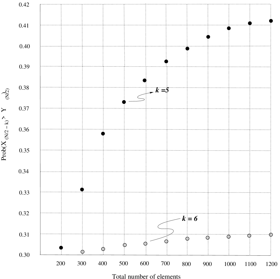
Figure 4: $P(X_{n-k}>Y_{n})$

We computed the value of $P(X_{n-k}>Y_{n})$ for various values of $n,N$ and $k$. The results are displayed in Figure 4. We note that:

1. $P(X_{n-k}>Y_{n})>k$, for a particular $k$, increases with $N$.

2. $P(X_{n-k}>Y_{n})>k$, for particular $N$, decreases with increasing $k$.

These observations are consistent with the experimental results displayed in Figures 2 and 3.

If the $n^{th}$ element in one of the merged sequences is less than the $(n-k)^{th}$ element in the other, then there exists a $D$ segment in the shuffled sequences of length $\geq 2k$. See Figure 5. At some point the algorithm is required to unpack this segment and rotate the $P-O$ segment, where $|P|\geq 1$. This requires at least $|D|+|O|+1$ moves, since $|P|\geq 1$, but can not guarantee no more than $|O|+1$ elements are now in their final locations. That is, $\geq 3k+1$ moves are needed to place $k+1$ elements. Since the frequency of occurrence of $D$ segments of length $2k$ increases with $N$ this causes the number of moves to be super-linear in $N$.

5 Conclusions

We have presented experimental results and a theoretical analysis showing that the time complexity of this algorithm is super-linear in $N$, even in the average case. Consequently, it does not improve on the original perfect shuffle based algorithm [3]. We suggest that it might be interesting to consider if the initial shuffling of the merged sequences necessarily introduces so much disorder that, on the average, the 2-ordered sequence can not be sorted in linear time.

Acknowledgement The authors wish to thank Julie Zhou for showing us how to use order statistics.

Appendix 1: The algorithm for equal length lists

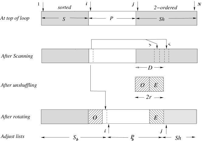
Figure 5: The three sub-arrays

Suppose the lists are of equal length. The process maintains three lists: a sorted list, $S$, an intermediate list, $P$ and a 2-ordered list, $Sh$. Figure 5 illustrates these structures. The array indices $i$ and $j$ are used to delineate the extents of the three lists. Index $i$ defines the beginning of $P$ and $j$ the beginning of $Sh$. The list $S$ comprises $A[1]$ - $A[i-1]$, $P$ is $A[i]$ - $A[j-1]$ and $Sh$ is $A[j]$ - $A[N]$.

The algorithm Right-going-merge, see Algorithm 1, uses four procedures. The procedure Scan returns an integer $r$ such that $A[j]$ - $A[j+2r-1]$ is a maximal, even length prefix of $Sh$, denoted $D$, such that all odd indexed elements are less than $A[i]$, the first element of $P$. Scan is only invoked if $|Sh|\geq 2$. The procedure Shuffle performs an in-shuffle on the input lists, assumed to be of equal length, i.e., only the interior elements are moved, the first and last elements are left unmoved. The procedure Unshuffle performs the inverse of Shuffle, i.e., an un-in-shuffle, on $D$ to produce the two lists $O$ and $E$. Shuffling methods are discussed in Section 4. The procedure Rotate circularly shifts the two adjacent segments of $A$ that represent $P$ and $O$ to the right by $r$. See Figure 5. We call this procedure right-going-merge because the scan proceeds from left to right. As described in Section 2.3, to handle the case where the lists are not of equal length, we also use the mirror image of this procedure, called the left-going-merge, which scans from right to left.

	Create $Sh$ by applying Shuffle to the two, equal length lists;
	{Recall that $A[i]$ is $P[1]$ and $A[j]$ is $Sh[1]$}
	$i:=$ index of first element in $Sh$; $j:=i+1$;
	while not $Sh$ is empty do
		if $P[1]<Sh[1]$ then {adjust lists} i := i+1
			if $|P|=0$ then $j:=j+1$; complement(type) fi
		else if $|Sh|=1$ then $r$ := 1; Rotate; {adjust lists} i := i+1; j:=j+1
		else {Figure 1} Scan; Unshuffle; Rotate;
			{Adjust lists} $i:=i+r+1;$ $j:=j+2r$ fi fi
	endwhile;

Algorithm 1: Right-going-merge

Appendix 2: The invalid proof

Lemma 5.1

If $r>0$ then $Pr(|D|=2r)\leq 1/2^{r}$.

Proof   
Let the number of elements in $P$, which are all from one list, say $L$, plus the number of $L$ elements in $Sh$, be $n$ and the number of $R$ elements in $Sh$ be $m$. The number of possible merged arrangements of these $n+m$ elements is $(n+m)!/(n!m!)$.

Suppose Scan defines $D$ such that $|D|=2r>0$. We note that $m\geq r$ and $n\geq m$. After the Unshuffle, Rotate and redefinition of the list, the number of $L$ elements in $P$ and $Sh$ is $n-1$ and the number of $R$ elements in $Sh$ is $m-r$. See Figure 5. The number of arrangements consistent with this fact is $(n+m-r-1)!/((n-1)!(m-r)!)$. Hence the probability that $|D|=2r$ is given by:

$$Pr(|D|=2r) = \frac{(n+m-r-1)!n!m!}{(m-r)!(n-1)!(n+m)!}$$

$$= \frac{n.m(m-1)\cdots(m-r+1)}{(n+m)(n+m-1)\cdots(n+m-r)}$$

$$= \frac{n}{n+m-r}\times\frac{m}{n+m}\times\frac{m-1}{n+m-1}\cdots\times\frac{m-r+1}{n+m-r+1}$$

$$\leq 1/2^{r}$$

because $m\geq r$ implies $n/(n+m-r)\leq 1$ and, for all $0\leq k$, $(m-k)/(n+m-k)\leq 1/2$. $\Box$

Let $P_{b}$ and $S_{b}$ be the $P$ and $S$ lists, respectively, at the bottom of the while loop, after all rearrangements and adjustments to the lists. See Figure 5.

Lemma 5.2

$Pr(|P_{b}|=p)\leq 1/2^{p-1}$.

Proof   
Suppose there are $n$ elements of type left and $m$ of type right distributed across $S_{b}$ and $P_{b}$. Then $m$ is within one of $n$ because the numbers of each type remaining in $Sh$ are within one of each other and the input lists were of equal length. The number of possible merged arrangements of these $m+n$ elements is $(m+n)!/(m!n!)$.

Without loss of generality, suppose the elements in $P_{b}$ are of type left. Then the number of arrangements consistent with the existence of $|P_{b}|=p$ elements all greater than any element in $S_{b}$ is the number of ways that $S_{b}$ can result from the merge of $n$ with $m-p$ elements, i.e., $(m+n-p)!/((m-p)!n!)$. Hence the probability that $|P_{b}|=p$ is given by:

$$Pr(|P_{b}|=p) = \frac{(m+n-p)!}{(m-p)!n!}\times\frac{m!n!}{(m+n)!}$$

$$= \frac{m(m-1)(m-2)\cdots(m-p+1)}{(m+n)(m+n-1)(m+n-2)\cdots(m+n-p+1)}$$

$$= \frac{m}{(m+n)}\times\frac{m-1}{m+n-1}\times\frac{m-2}{m+n-2}\cdots\times\frac{m-p+1}{m+n-p+1}$$

$$\leq 1/2^{p-1}$$

because $m/(m+n)<1$ and, for all $0\leq k<n$, $(m-k)/(m+n-k)\leq 1/2$. $\Box$

Lemmas 5.1 and 5.2 allow us to show that the expected time complexity of all the loop procedures is a constant.

Lemma 5.3

The expected time used by the Scan procedure is constant.

Proof   
The time taken to scan $2r$ elements is $k_{1}r$, for some constant $k_{1}$. Hence the expected time, expt-scan, is given by:

expt-scan $$= \sum_{r}k_{1}rPr(|D|=2r)\leq\sum_{r=1}^{\infty}k_{1}r/2^{r}=2k_{1},$$

by Lemma 5.1. $\Box$

Because element comparisons are restricted to the Scan procedure, Lemma 5.3 tells us that the average number of comparisons per loop traversal is a constant.

Lemma 5.4

The expected time used by the unShuffle procedure is constant.

Proof   
The time required to Unshuffle a list $D$, where $|D|=2r$, is $k_{2}r$, for some constant $k_{2}$. See Section 4 below. Hence the expected time, expt-shuff, is given by:

expt-shuff $$= \sum_{r}k_{2}rPr(|D|=2r)\leq\sum_{r=1}^{\infty}k_{2}r/2^{r}=2k_{2},$$

by Lemma 5.1 and the fact that the unshuffle works on the result of the scan. $\Box$

Lemma 5.5

The expected time used by the Rotate procedure is constant.

Proof   
$P_{b}+1$ elements are rotated, where $P_{b}$ is list $P$ at the bottom of the loop, i.e., after rotation. The time taken to rotate $|P_{b}|+1$ elements is $\leq(|P_{b}|+1)k_{3}$, for some constant $k_{3}$. Hence the expected time, expt-rot, is given by:

expt-rot $$= \sum_{p}(p+1)k_{3}Pr(|P_{b}|=p)\leq\sum_{p=1}^{\infty}(p+1)k_{3}/2^{p}=\sum_{p=1}^{\infty}pk_{3}/2^{p}+\sum_{p=1}^{\infty}k_{3}/2^{p}=3k_{3},$$

by Lemma 5.2. $\Box$

Because element moves are restricted to the Unshuffle and Rotate procedures, Lemmas 5.4 and 5.5 tell us that the average number of moves per loop traversal is a constant.

Theorem 5.1

The average time complexity of the algorithm is $O(n)$, where $n$ is the combined length of the two input lists.

Proof   
Consider the merge procedures. The actions inside the loop are either constant time operations or scans, rotations or unshuffles which, by Lemmas 5.3, 5.4, 5.5 and the “linearity of expectations” [1, Appendix C], are expected constant time operations. Hence the expected time to traverse the while loop is a constant.

Now consider the general case where the problem is broken down to the merge of a sequence of equal length lists of lengths say $n_{1}$, $n_{2}\ldots n_{k}$. We observe that $\sum_{i=1}^{k}n_{i}=n$. Since each merge takes time $O(n_{i})$, the total time is $O(n)$. $\Box$

References

- [1] Thomas H. Cormen. Introduction to Algorithms. Cambridge, 2001.
- [2] Mehmet Emin Dalkiliç, Elif Acar, and Gorkem Tokatli. A simple shuffle-based stable in-place merge algorithm. Procedia CS, 3:1049–1054, 2011.
- [3] John Ellis and Minko Markov. In situ, stable merging by way of the perfect shuffle. The Computer Journal, 43:40–53, 2000.
- [4] John Ellis and Ulrike Stege. A provably, linear time, in-place and stable merge algorithm via the perfect shuffle. CoRR, 1508.00292, 2015.