Probing $Zt\bar{t}$ couplings using $Z$ boson polarization in $ZZ$ production at hadron colliders

Abstract

We propose to utilize the polarization information of the $Z$ bosons in $ZZ$ production, via the gluon-gluon fusion process $gg\to ZZ$, to probe the $Zt\bar{t}$ gauge coupling. The contribution of longitudinally polarized $Z$ bosons is sensitive to the axial-vector component ($a_{t}$) of the $Zt\bar{t}$ coupling. We demonstrate that the angular distribution of the charged lepton from $Z$ boson decays serves well for measuring the polarization of $Z$ bosons and the determination of $a_{t}$. We show that $ZZ$ production via the $gg\to ZZ$ process complement to $Zt\bar{t}$ and $tZj$ productions in measuring the $Zt\bar{t}$ coupling at hadron colliders.

1. Introduction.

Top quark, the heaviest fermion in the Standard Model (SM), is commonly believed to be sensitive to new physics (NP) beyond the SM. The top quark often plays a key role in triggering electroweak symmetry breaking (EWSB) in many NP models, and as a result, the gauge couplings of top quarks, e.g. $Wtb$ and $Zt\bar{t}$, may largely deviate from the SM predictions Martin (1997); Contino (2011); Bellazzini et al. (2014); Panico and Wulzer (2016); Csaki and Tanedo (2015). The $Wtb$ couplings have been well measured in both the single top quark production and the top-quark decay Chen et al. (2005); Prasath V et al. (2015); Cao et al. (2017); Romero Aguilar et al. (2015); Hioki and Ohkuma (2016); Buckley et al. (2016); Zhang (2016); Birman et al. (2016); Jueid (2018); Cao et al. (2018); Sun et al. (2019); Cao et al. (2019); the $Zt\bar{t}$ coupling can be measured in $t\bar{t}Z$ and $tjZ$ productions Baur et al. (2005); Campbell et al. (2013); Rontsch and Schulze (2014); Cao and Yan (2015); Bessidskaia Bylund et al. (2016); Berger et al. (2009); Degrande et al. (2018); Martini and Schulze (2020) which are, unfortunately, difficult to separately determine the vector and axial-vector components of the $Zt\bar{t}$ coupling. The chiral structure of the $Zt\bar{t}$ coupling would reveal the gauge structure of NP models Richard (2014); Cao and Yan (2015), therefore, measuring and distinguishing the vector and axial vector components of the $Zt\bar{t}$ coupling is in order.

In this work we explore the potential of measuring the $Zt\bar{t}$ coupling using the polarization information of the $Z$ bosons in $ZZ$ production, at the CERN Large Hadron Collider (LHC). The $Zt\bar{t}$ coupling contributes to $ZZ$ production through top-quark loop effects in the gluon fusion channel. The process, $gg\to ZZ$, has been used to constrain the Higgs boson width through the interference of box and triangle diagrams and it has been shown to be sensitive to many NP effects Caola and Melnikov (2013); Chen et al. (2014); Campbell et al. (2014); Coleppa et al. (2014); Gainer et al. (2015); Azatov et al. (2015); Englert et al. (2015a); Li et al. (2015); Englert et al. (2015b); Azatov et al. (2016); Goncalves et al. (2018a); Lee et al. (2019a); Goncalves et al. (2018b); He et al. (2019). In particular, the polarization of the $Z$ boson pair highly depends on the $Zt\bar{t}$ coupling. The polarizations of $Z$ bosons in $ZZ$ pair production can be categorized as: TT (transverse-transverse), TL (transverse-longitudinal), and LL (longitudinal-longitudinal).

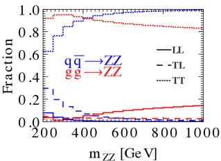
Figure 1: The fractions of three polarization modes in the processes of $gg\to ZZ$ and $q\bar{q}\to ZZ$ at the 13 TeV LHC.

Figure 1 shows the fraction of the three polarization modes of $ZZ$ pairs in the processes of $gg\to ZZ$ (red) and $q\bar{q}\to ZZ$ (blue) at the 13 TeV LHC. The TT mode dominates in both production processes as a result of that, owing to the Goldstone boson equivalence theorem, the interaction of the longitudinal mode to light quarks is highly suppressed by the small mass of the light quarks. The suppression of the LL mode in the $gg\to ZZ$ channel arises from the cancellation between the box and triangle diagrams due to unitarity, and the cancellation is sensitive to the axial-vector coupling of $Zt\bar{t}$ Glover and van der Bij (1989). In the high energy limit, the contribution of top-quark loops to the LL mode is given by

$$M_{\pm,\pm,0,0}\sim\frac{m_{t}^{2}}{m_{Z}^{2}}\left(a_{t}^{2}-\frac{1}{4}\right)\left[\log^{2}\left(\frac{\hat{s}}{m_{t}^{2}}\right)-2i\pi\log\left(\frac{\hat{s}}{m_{t}^{2}}\right)\right],$$ (1)

where $a_{t}$ is the axial-vector component of the $Zt\bar{t}$ coupling, $m_{t}$ and $m_{Z}$ denotes the mass of the top quark and $Z$ boson, respectively. The subscript $+$, $-$ and $0$ denote the right-handed, left-handed and longitudinal polarization of the gluons or $Z$ bosons, respectively. In the SM, $a_{t}=1/2$, and it yields a strong cancellation in the LL mode scattering. However, in the NP model the value of $a_{t}$ can deviate from its SM value, so that the above-mentioned cancellation is spoiled and the fraction of the LL mode contribution would be enhanced. Therefore, the polarization information of the $Z$ boson pairs in $ZZ$ production, via $gg\to ZZ$, can be used to probe the axial-vector coupling of $Zt\bar{t}$ interaction at hadron colliders.

2. $ZZ$ production via Gluon fusion.

Here, we consider the case that the NP effects modify only the four-dimensional $Zt\bar{t}$ coupling. The effective Lagrangian of the $Zt\bar{t}$ interaction is

$$\mathcal{L}=\frac{g_{W}}{2c_{W}}\bar{t}(v_{t}-a_{t}\gamma_{5})\gamma_{\mu}t,$$ (2)

where $g_{W}$ is the electroweak gauge coupling and $c_{W}$ is the cosine of the weak mixing angle $\theta_{W}$. In the SM,

$$v_{t}^{\rm SM}=\frac{1}{2}-\frac{2}{3}s_{W}^{2}=0.3526,\quad a_{t}^{\rm SM}=\frac{1}{2},$$ (3)

where $s_{W}\equiv\sin\theta_{W}$. We calculate the helicity amplitudes of the channel $g(\lambda_{1})g(\lambda_{2})\to Z(\lambda_{3})Z(\lambda_{4})$ using FeynArts and FeynCalc Hahn (2001); Shtabovenko et al. (2016) where $\lambda_{i}$ labels the helicity of particle $i$. The contribution of the box diagram ($\square$) to each helicity amplitude can be parametrized as Glover and van der Bij (1989),

$$M^{\square}_{\lambda_{1},\lambda_{2},\lambda_{3},\lambda_{4}} =\left(v_{t}^{2}+a_{t}^{2}\right)A_{\lambda_{1},\lambda_{2},\lambda_{3},\lambda_{4}}$$

$$+\left(v_{t}^{2}-a_{t}^{2}\right)B_{\lambda_{1},\lambda_{2},\lambda_{3},\lambda_{4}}$$

$$+a_{t}^{2}C_{\lambda_{1},\lambda_{2},\lambda_{3},\lambda_{4}},$$ (4)

where $\lambda_{i}=\pm$ and $0$. Both $B_{\lambda_{1},\lambda_{2},\lambda_{3},\lambda_{4}}$ and $C_{\lambda_{1},\lambda_{2},\lambda_{3},\lambda_{4}}$ vanish for (massless) light quark loops. In the limit of $\hat{s}=-\hat{t}/2=-\hat{u}/2\gg m_{t}$, where $\hat{s},\hat{t}$ and $\hat{u}$ are the usual Mandelstam variables, the coefficients $A,B$ and $C$ are

$$A\sim\text{Constant},$$

$$B\sim 0,$$

$$C_{\pm,\pm,0,0}\sim-\frac{m_{t}^{2}}{m_{Z}^{2}}\left[\log^{2}\left(\frac{\hat{s}}{m_{t}^{2}}\right)-2i\pi\log\left(\frac{\hat{s}}{m_{t}^{2}}\right)\right].$$ (5)

Here, the constant in the coefficient $A$ is a combination of gauge couplings and loop factor. Furthermore, The contribution of the triangle diagram ($\bigtriangleup$) to each helicity amplitude is

$$M_{\pm,\pm,0,0}^{\bigtriangleup}\sim\frac{m_{t}^{2}}{4m_{Z}^{2}}\left[\log^{2}\left(\frac{\hat{s}}{m_{t}^{2}}\right)-2i\pi\log\left(\frac{\hat{s}}{m_{t}^{2}}\right)\right],$$ (6)

which cancels with the coefficient $C$ in the contribution of the box diagram $M^{\square}$ for each helicity amplitude. The sensitivity of the cancellation on $a_{t}$ can be understood from the fact that the axial current is not conserved for the top quark, whose mass is at the weak scale.

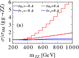
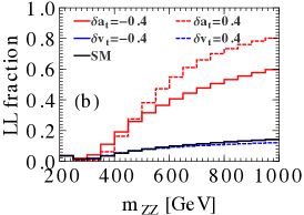
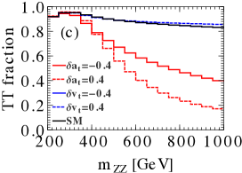
Figure 2: (a) The differential cross section of $gg\to ZZ$ for various $\delta v_{t}$’s and $\delta a_{t}$’s, normalized to the SM prediction, as a function of $m_{ZZ}$ at the 13 TeV LHC; the polarization fraction of the LL mode (b) and the TT mode (c).

Below, we consider the impact of the non-standard $Zt\bar{t}$ coupling to the differential cross sections of $gg\to ZZ$ by changing only one parameter at a time. Both of the light and top quark loop contributions have been included in our numerical calculation. The light quark loop contribution gives the dominant contribution to the inclusive cross section, while it is only sensitive to the TT mode of the $ZZ$ pairs. Any deviation in the LL mode of the inclusive cross section, as studied in this work, can only come from the non-standard $Zt\bar{t}$ coupling. Furthermore, we have compared the result of our numerical calculations with that using the MadGraph5 code Alwall et al. (2014) and found excellent agreement.

Define $\delta v_{t}$ and $\delta a_{t}$ as the amount of deviation of the vector and axial-vector couplings from the SM values, i.e.,

$$\delta v_{t}=v_{t}-v_{t}^{\rm SM},\quad\delta a_{t}=a_{t}-a_{t}^{\rm SM}.$$ (7)

Figure 2(a) shows the differential cross sections of $gg\to ZZ$, normalized to the SM prediction, as a function of the invariant mass of the $Z$ boson pair ($m_{ZZ}$) for various $\delta v_{t}$’s and $\delta a_{t}$’s at the 13 TeV LHC. Figure 2(b) and (c) show the fraction of the LL and TT modes as a function of $m_{ZZ}$, respectively. The TL mode is not plotted as it is quite small in comparison with the LL and TT modes. The LL model is very sensitive to the anomalous $a_{t}$ coupling; for example, the contribution of the LL mode increases dramatically in the large $m_{ZZ}$ region for $\delta a_{t}=\pm 0.4$, cf. the red solid and red dashed curves. On the other hand, the LL mode is not sensitive to $\delta v_{t}$. The fractions of the LL and TT modes are slightly altered for the choice of $\delta v_{t}=\pm 0.4$ and are very close to their fractions in the SM; cf. the blue and black curves. Therefore, the polarization information of the $Z$ bosons in $ZZ$ production can be utilized to provide a good probe of the anomalous $a_{t}$ coupling.

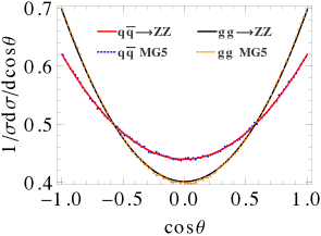
Figure 3: The $\cos\theta$ distribution, of the processes $gg,{q\bar{q}}\to ZZ\to 4\ell$ in the SM, where the solid and dotted curves denote the theory template and the MC simulation, respectively, without imposing any kinematic cut.

The polarization information of the final state $Z$ boson can be inferred from the angular distribution ($\cos\theta$) of the charged lepton in the rest frame of the $Z$ boson from which the charged lepton is emitted. The angular distributions for various polarization states of the $Z$ boson are given as

$$\phi_{L}(\cos\theta)=\frac{3}{4}(1-\cos^{2}\theta),~{}\phi_{T}(\cos\theta)=\frac{3}{8}(1+\cos^{2}\theta),$$ (8)

where $\phi_{L}$ denotes a longitudinally polarized $Z$ boson, and $\phi_{T}$ a transversely polarized $Z$. The angle $\theta$ is defined as the opening angle between the charged lepton three-momentum in the rest frame of the $Z$-boson and the $Z$-boson three-momentum in the center of mass frame of the $ZZ$ pair.

To determine the value of $a_{t}$, we compare the angular distributions ($\cos\theta$) predicted by the Monte Carlo (MC) simulation to the theory template obtained by the analytical calculation. The theory template of $\cos\theta$ distribution, of the processes $gg,{q\bar{q}}\to ZZ\to 4\ell$ with $\ell=e^{\pm},\mu^{\pm}$, is approximated by multiplying the fraction of each polarization mode of the $ZZ$ boson pair with the corresponding $\phi_{L,T}$ distributions. Though the spin correlation between the two final-state $Z$ bosons is not strictly maintained in this approximation, the prediction of the theory template (solid curves) on the $\cos\theta$ distribution, via either the $q\bar{q}$ or $gg$ scattering process, in the SM agrees very well with that obtained by the MC simulation (dashed curves), as clearly shown in Figure 3 without imposing any kinematic cut.

3. Collider simulation.

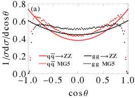
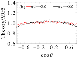
Figure 4: (a) The $\cos\theta$ distribution, of the processes $gg,{q\bar{q}}\to ZZ\to 4\ell$ in the SM, after imposing the kinematic cuts as described in the main text. The solid curves represents the theory template and the dotted curves denotes the MC simulation; (b) The ratio between the prediction of theory template and the MC data for $|\cos\theta|<0.8$.

Next we perform a detailed Monte Carlo simulation to explore the potential of probing $a_{t}$ via the signal process $gg\to ZZ\to 4\ell$ at the 13 TeV LHC and a 100 TeV proton-proton (pp) hadron collider. Its major background comes from the process $q\bar{q}\to ZZ$, while the other backgrounds are negligible Aaboud et al. (2018). We generate both the signal and background events by MadGraph5 Alwall et al. (2014) at the parton-level and pass events to PYTHIA Sjostrand et al. (2008) for showering and hadronization. The Delphes package is used to simulate the detector smearing effects de Favereau et al. (2014). The QCD corrections are taken into account by introducing a constant $\kappa$ factor, i.e. $\kappa_{gg}=1.8$ and $\kappa_{q\bar{q}}=1.7$ Caola et al. (2015); Cascioli et al. (2014); Heinrich et al. (2018); Grazzini et al. (2019); Kallweit and Wiesemann (2018); Agarwal and Von Manteuffel (2019). At the analysis level, both the signal and background events are required to pass the kinematic cuts: $|\eta_{\ell}|<2.5$ and $P_{T\ell}>15~{}{\rm GeV}$. We further require the invariant mass window cut for same flavor leptons as $80<m_{\ell\ell}<100~{}{\rm GeV}$ and demand $m_{4\ell}>600~{}{\rm GeV}$ to enhance the LL mode.

The kinematic cuts inevitably modify the lepton kinematics and the polarization fractions of the $ZZ$ bosons. In this study, we require $m_{ZZ}>600~{}{\rm GeV}$ and $|\eta_{Z}|<2$. Figure 4(a) displays the $\cos\theta$ distribution after imposing the kinematic cuts for the processes $gg\to ZZ$ (black) and $q\bar{q}\to ZZ$ (red). The shapes of the $\cos\theta$ distributions of the theory template agree with those of the MC simulation (labeled as MG5 in Fig. 4) except near the edge region. Note that the predictions of MG5 have included the effects from parton shower and detector level simulation. Focusing on the central region with $|\cos\theta|<0.8$, we plot the ratio between the normalized theory template and the MC simulation in Fig 4(b), which shows good agreements between the two calculations. Hence, we applied the cut of $|\cos\theta|<0.8$ in the following analysis, when using only the theory template predictions.

The total event number of the signal ($N_{s}$) and background ($N_{b}$) processes are

$$N_{s}= \sigma(gg\to ZZ)\times 4{\rm Br}^{2}\times\epsilon_{\rm cut}^{g}\times\mathcal{L}_{\rm int},$$

$$N_{b}= \sigma(q\bar{q}\to ZZ)\times 4{\rm Br}^{2}\times\epsilon_{\rm cut}^{q}\times\mathcal{L}_{\rm int},$$ (9)

where $\epsilon_{\rm cut}^{g,q}$ is the cut efficiency for the signal and background process, respectively. $\mathcal{L}_{\rm int}$ is the integrated luminosity, and

$${\rm Br}\equiv{\rm Br}(Z\to e^{+}e^{-})={\rm Br}(Z\to\mu^{+}\mu^{-}).$$ (10)

In the SM (with $\delta v_{t}=\delta a_{v}=0$), the total cross section of the signal ($\sigma_{s}$) and background ($\sigma_{b}$) processes are,

$$\sigma_{s}=\sigma(gg\to ZZ)\times 4{\rm Br}^{2}\times\epsilon_{\rm cut}^{g}\simeq 0.032~{}{\rm fb},$$

$$\sigma_{b}=\sigma(q\bar{q}\to ZZ)\times 4{\rm Br}^{2}\times\epsilon_{\rm cut}^{q}\simeq 0.2~{}{\rm fb}$$ (11)

at the 13 TeV LHC, while at a 100 TeV pp collider

$$\sigma_{s}=\sigma(gg\to ZZ)\times 4{\rm Br}^{2}\times\epsilon_{\rm cut}^{g}\simeq 1.26~{}{\rm fb},$$

$$\sigma_{b}=\sigma(q\bar{q}\to ZZ)\times 4{\rm Br}^{2}\times\epsilon_{\rm cut}^{q}\simeq 1.72~{}{\rm fb}.$$ (12)

There are roughly about 700 and 9000 events of $ZZ$ pairs produced at the 13 TeV LHC and a 100 TeV pp collider with an integrated luminosity of $3000~{}{\rm fb}^{-1}$.

For probing the $Zt\bar{t}$ coupling, we divide the $|\cos\theta|$ distribution into 8 bins and use the binned likelihood function to estimate the sensitivity for the hypothesis of NP with a non-vanishing $(\delta v_{t},\delta a_{t})$ against the hypothesis of the SM coupling Cowan et al. (2011),

$$L(\delta v_{t},\delta a_{t})=\prod_{i=1}^{N_{\rm bin}}\frac{(s_{i}(\delta v_{t},\delta a_{t})+b_{i})^{n_{i}}}{n_{i}!}e^{-s_{i}(\delta v_{t},\delta a_{t})-b_{i}},$$ (13)

where $n_{i}$ denotes the number of observed events in the $i$th bin, $b_{i}$ the number of background events, and $s_{i}(\delta v_{t},\delta a_{t})$ the number of signal events with the anomalous coupling $(\delta v_{t},\delta a_{t})$. The observed event is assumed to be $n_{i}=b_{i}+s_{i}(0,0)$. The numbers of the signal events ($s_{i}$) and the background events ($b_{i}$) in each bin are determined by the total cross section, the fraction of polarization modes of the $Z$ boson pair and the $\phi_{L,T}$ functions, i.e.,

$$s_{i}(\delta v_{t},\delta a_{t}),b_{i}=F_{N}^{g,q}N_{s,b}\int_{i}d\cos\theta\left[R_{L}^{g,q}\phi_{L}+(1-R_{L}^{g,q})\phi_{T}\right],$$ (14)

where $R_{L}^{g,q}$ is the fraction of a longitudinal polarized $Z$ boson, which decays into a pair of electron or muon leptons, in the scattering processes $gg\to ZZ$ and $q\bar{q}\to ZZ$, respectively. Here, $F_{N}^{g,q}$ is the normalization factor to ensure that $F_{N}^{g,q}\int_{-0.8}^{0.8}d\cos\theta\left[R_{L}^{g,q}\phi_{L}+(1-R_{L}^{g,q})\phi_{T}\right]=1.$ Explicitly, $F_{N}^{g,q}=1/(0.728+0.216R_{L}^{g,q})$. Define the likelihood function ratio as following,

$$q^{2}=-2\frac{L(\delta v_{t},\delta a_{t})}{L(0,0)},$$ (15)

which describes the exclusion of the hypothesis of NP with non-zero $(\delta v_{t},\delta a_{t})$ versus the hypothesis of SM at the $q$-sigma ($q\sigma$) level.

Figure 5 displays the projected regions of the parameter space in which $(\delta v_{t},\delta a_{t})$ can be measured at the $2\sigma$ level, at the 13 TeV LHC and a 100 TeV pp hadron collider with an integrated luminosity of $3000~{}\rm{fb}^{-1}$. The cyan and gray regions denote the constraints provided by the measurement of $tZj$ Aad et al. (2020); Sirunyan et al. (2019) and $Zt\bar{t}$ Sirunyan et al. (2020); Aaboud et al. (2019) productions at the 13 TeV LHC, respectively. The horizontal black line represents the upper limit of $\delta a_{t}$ derived from the strength of the off-shell Higgs-boson signal in $ZZ$ production Aaboud et al. (2018). The purple region denotes the projected parameter space obtained from measuring the degree of polarization of the $Z$ bosons in $gg\to ZZ$ production, at the $2\sigma$ level, at the 13 TeV LHC, while the orange region is the projected parameter space for a 100 TeV pp collider.

It is evident that the measurement of $Zt\bar{t}$ production, as compared to $ZZ$ and $tZj$ productions, yields the strongest constraint on values of $\delta v_{t}$ and $\delta a_{t}$ at the 13 TeV LHC. However, the drawback of this measurement is that the bounded region contains a degeneracy of $\delta a_{t}$ and $\delta v_{t}$, i.e.

$$0.77\leq 3.05\left(\delta a_{t}+0.5\right)^{2}+1.71\left(\delta v_{t}+0.19\right)^{2}\leq 1.14.$$ (16)

Taking into account the $tZj$ production can partially resolve the degeneracy, found in analyzing the $Zt\bar{t}$ events. The $ZZ$ production is sensitive only to $a_{t}$, and it alone yields a twofold constraint $\delta a_{t}\in[-0.25,0.15]\cup[-1.16,-0.75]$ at the 13 TeV LHC, and $\delta a_{t}\in[-0.08,0.06]\cup[-1.00,-0.92]$ at a 100 TeV pp collider, cf. the two purple and orange regions. With a larger data sample in the future runs of the LHC and a 100 TeV pp collider, it is possible to precisely determine first the axial-vector component $a_{t}$, and then the vector component $v_{t}$ of the $Zt\bar{t}$ coupling. The measurement of $tZj$ production is particularly important for the determination of its vector component from the combined analysis. It was shown in Ref. Mangano et al. (2017); Vos (2017) that at a 100 TeV pp collider, the measurement of the $Zt\bar{t}$ coupling could be further improved by studying the $t\bar{t}Z$ and $tjZ$ production cross sections and its uncertainty can be controlled to within a few percent level.

Before closing this section, we would like to compare our findings, derived from studying the polarization state of the produced $ZZ$ pairs from $gg$ fusion, with that in the literature, obtained from studying the inclusive production rates alone. In Ref. Azatov et al. (2016), it was concluded that $a_{t}$ can be constrained as $\delta a_{t}/a_{t}\in[-0.42,0.35]$ by measuring the $gg\to ZZ$ inclusive cross section at the 14 TeV LHC with an integrated luminosity of $3~{}\rm{ab}^{-1}$. With $a_{t}^{\rm SM}=0.5$, the result of our analysis, invoking the polarization information of the final state $ZZ$ pairs, yields $\delta a_{t}/a_{t}\in[-0.44,0.3]$, though it is for a 13 TeV LHC. It appears that our result only slightly improve the sensitivity of this production channel to the measurement of the $Zt\bar{t}$ coupling. However, the main point made and demonstrated in this work is that the LL mode of the $ZZ$ pair production is sensitive to the anomalous $a_{t}$ (but not $v_{t}$) coupling of top quark to $Z$ boson. Hence, it can be used to help disentangle the contributions of both $a_{t}$ and $v_{t}$ couplings in the total inclusive cross section measurement. Moreover, the result presented in this work could potentially be improved if one utilizes advanced technologies such as Boosted Decision Tree or Multi-Variable Analysis Lee et al. (2019a, b), which is however beyond the scope of this work.

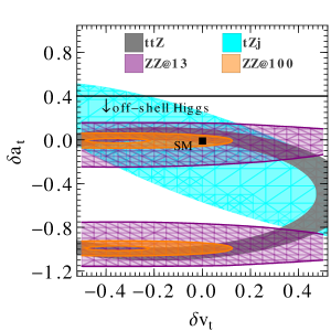
Figure 5: The parameter space of $(\delta v_{t},\delta a_{t})$, to be constrained by the measurement of $ZZ$ production, at the $2\sigma$ level at the 13 TeV LHC (purple region) and a 100 TeV pp hadron collider (orange region), respectively, with an integrated luminosity of $3000~{}\rm{fb}^{-1}$. The gray region represents the present constraint from the $Zt\bar{t}$ production Aaboud et al. (2019); Sirunyan et al. (2020), and the cyan region from the $tZj$ production Sirunyan et al. (2019); Aad et al. (2020) at the 13 TeV LHC.

4. Summary.

We propose to measure the axial-vector component of the $Zt\bar{t}$ coupling by utilizing the polarization information of the $Z$ bosons in the process $gg\to ZZ$, at the 13 TeV LHC and a 100 TeV proton-proton collider. When the final-state $Z$-bosons are both longitudinally polarized, the cross section for $gg\to ZZ$ is sensitive to the axial-vector coupling $a_{t}$, because the axial current is not conserved for massive top quarks. We demonstrate that the fraction of longitudinal-longitudinal (LL) mode increases with a non-vanishing anomalous coupling $a_{t}$, when the invariant mass of the $Z$-boson pair becomes larger. From the angular distribution of the charged leptons from the $Z$-boson decay, one can determine the polarization of the $Z$ bosons and in turn to probe the anomalous $a_{t}$ coupling, regardless of the value of the vector component ($v_{t}$) of the $Zt\bar{t}$ coupling. By comparing the theory template and Monte Carlo simulation, we find the parameter space of $\delta a_{t}\equiv a_{t}-a_{t}^{\rm SM}$ which can be probed at the $2\sigma$ level, from the measurement of $ZZ$ production at hadron colliders. It is $\delta a_{t}\in[-0.25,0.15]\cup[-1.16,-0.75]$ at the 13 TeV LHC, and $\delta a_{t}\in[-0.08,0.06]\cup[-1.00,-0.92]$ at a 100 TeV pp collider. We emphasize that the $ZZ$ production is complementary to the $Zt\bar{t}$ and $tZj$ productions in the measurement of the $Zt\bar{t}$ coupling.

Acknowledgments. BY thank Yandong Liu, Zhuoni Qian and Ling-Xiao Xu for helpful discussion. QHC and YZ are supported in part by the National Science Foundation of China under Grant Nos. 11725520, 11675002 and 11635001. BY was supported by the U.S. Department of Energy through the Office of Science, Office of Nuclear Physics under Contract DE-AC52-06NA25396 and by an Early Career Research Award (C. Lee). C.-P. Yuan was supported by the U.S. National Science Foundation under Grant No. PHY-1719914. C.-P. Yuan is also grateful for the support from the Wu-Ki Tung endowed chair in particle physics.

References

- Martin (1997) S. P. Martin, pp. 1–98 (1997), [Adv. Ser. Direct. High Energy Phys.18,1(1998)], eprint hep-ph/9709356.
- Contino (2011) R. Contino, in Physics of the large and the small, TASI 09, proceedings of the Theoretical Advanced Study Institute in Elementary Particle Physics, Boulder, Colorado, USA, 1-26 June 2009 (2011), pp. 235–306, eprint 1005.4269.
- Bellazzini et al. (2014) B. Bellazzini, C. Csaki, and J. Serra, Eur. Phys. J. C74, 2766 (2014), eprint 1401.2457.
- Panico and Wulzer (2016) G. Panico and A. Wulzer, Lect. Notes Phys. 913, pp.1 (2016), eprint 1506.01961.
- Csaki and Tanedo (2015) C. Csaki and P. Tanedo, in Proceedings, 2013 European School of High-Energy Physics (ESHEP 2013): Paradfurdo, Hungary, June 5-18, 2013 (2015), pp. 169–268, eprint 1602.04228.
- Chen et al. (2005) C.-R. Chen, F. Larios, and C. P. Yuan, Phys. Lett. B631, 126 (2005), eprint hep-ph/0503040.
- Prasath V et al. (2015) A. Prasath V, R. M. Godbole, and S. D. Rindani, Eur. Phys. J. C75, 402 (2015), eprint 1405.1264.
- Cao et al. (2017) Q.-H. Cao, B. Yan, J.-H. Yu, and C. Zhang, Chin. Phys. C41, 063101 (2017), eprint 1504.03785.
- Romero Aguilar et al. (2015) R. Romero Aguilar, A. O. Bouzas, and F. Larios, Phys. Rev. D92, 114009 (2015), eprint 1509.06431.
- Hioki and Ohkuma (2016) Z. Hioki and K. Ohkuma, Phys. Lett. B752, 128 (2016), eprint 1511.03437.
- Buckley et al. (2016) A. Buckley, C. Englert, J. Ferrando, D. J. Miller, L. Moore, M. Russell, and C. D. White, JHEP 04, 015 (2016), eprint 1512.03360.
- Zhang (2016) C. Zhang, Phys. Rev. Lett. 116, 162002 (2016), eprint 1601.06163.
- Birman et al. (2016) J. L. Birman, F. Deliot, M. C. N. Fiolhais, A. Onofre, and C. M. Pease, Phys. Rev. D93, 113021 (2016), eprint 1605.02679.
- Jueid (2018) A. Jueid, Phys. Rev. D98, 053006 (2018), eprint 1805.07763.
- Cao et al. (2018) Q.-H. Cao, P. Sun, B. Yan, C. P. Yuan, and F. Yuan, Phys. Rev. D98, 054032 (2018), eprint 1801.09656.
- Sun et al. (2019) P. Sun, B. Yan, and C. P. Yuan, Phys. Rev. D99, 034008 (2019), eprint 1811.01428.
- Cao et al. (2019) Q.-H. Cao, P. Sun, B. Yan, C. P. Yuan, and F. Yuan (2019), eprint 1902.09336.
- Baur et al. (2005) U. Baur, A. Juste, L. H. Orr, and D. Rainwater, Phys. Rev. D71, 054013 (2005), eprint hep-ph/0412021.
- Campbell et al. (2013) J. Campbell, R. K. Ellis, and R. Rontsch, Phys. Rev. D 87, 114006 (2013), eprint 1302.3856.
- Rontsch and Schulze (2014) R. Rontsch and M. Schulze, JHEP 07, 091 (2014), [Erratum: JHEP09,132(2015)], eprint 1404.1005.
- Cao and Yan (2015) Q.-H. Cao and B. Yan, Phys. Rev. D92, 094018 (2015), eprint 1507.06204.
- Bessidskaia Bylund et al. (2016) O. Bessidskaia Bylund, F. Maltoni, I. Tsinikos, E. Vryonidou, and C. Zhang, JHEP 05, 052 (2016), eprint 1601.08193.
- Berger et al. (2009) E. L. Berger, Q.-H. Cao, and I. Low, Phys. Rev. D80, 074020 (2009), eprint 0907.2191.
- Degrande et al. (2018) C. Degrande, F. Maltoni, K. Mimasu, E. Vryonidou, and C. Zhang, JHEP 10, 005 (2018), eprint 1804.07773.
- Martini and Schulze (2020) T. Martini and M. Schulze, JHEP 04, 017 (2020), eprint 1911.11244.
- Richard (2014) F. Richard (2014), eprint 1403.2893.
- Caola and Melnikov (2013) F. Caola and K. Melnikov, Phys. Rev. D88, 054024 (2013), eprint 1307.4935.
- Chen et al. (2014) M. Chen, T. Cheng, J. S. Gainer, A. Korytov, K. T. Matchev, P. Milenovic, G. Mitselmakher, M. Park, A. Rinkevicius, and M. Snowball, Phys. Rev. D89, 034002 (2014), eprint 1310.1397.
- Campbell et al. (2014) J. M. Campbell, R. K. Ellis, and C. Williams, JHEP 04, 060 (2014), eprint 1311.3589.
- Coleppa et al. (2014) B. Coleppa, T. Mandal, and S. Mitra, Phys. Rev. D90, 055019 (2014), eprint 1401.4039.
- Gainer et al. (2015) J. S. Gainer, J. Lykken, K. T. Matchev, S. Mrenna, and M. Park, Phys. Rev. D91, 035011 (2015), eprint 1403.4951.
- Azatov et al. (2015) A. Azatov, C. Grojean, A. Paul, and E. Salvioni, Zh. Eksp. Teor. Fiz. 147, 410 (2015), [J. Exp. Theor. Phys.120,354(2015)], eprint 1406.6338.
- Englert et al. (2015a) C. Englert, Y. Soreq, and M. Spannowsky, JHEP 05, 145 (2015a), eprint 1410.5440.
- Li et al. (2015) C. S. Li, H. T. Li, D. Y. Shao, and J. Wang, JHEP 08, 065 (2015), eprint 1504.02388.
- Englert et al. (2015b) C. Englert, I. Low, and M. Spannowsky, Phys. Rev. D91, 074029 (2015b), eprint 1502.04678.
- Azatov et al. (2016) A. Azatov, C. Grojean, A. Paul, and E. Salvioni, JHEP 09, 123 (2016), eprint 1608.00977.
- Goncalves et al. (2018a) D. Goncalves, T. Han, and S. Mukhopadhyay, Phys. Rev. Lett. 120, 111801 (2018a), [Erratum: Phys. Rev. Lett.121,no.7,079902(2018)], eprint 1710.02149.
- Lee et al. (2019a) S. J. Lee, M. Park, and Z. Qian, Phys. Rev. D100, 011702 (2019a), eprint 1812.02679.
- Goncalves et al. (2018b) D. Goncalves, T. Han, and S. Mukhopadhyay, Phys. Rev. D98, 015023 (2018b), eprint 1803.09751.
- He et al. (2019) H.-R. He, X. Wan, and Y.-K. Wang (2019), eprint 1902.04756.
- Glover and van der Bij (1989) E. W. N. Glover and J. J. van der Bij, Nucl. Phys. B321, 561 (1989).
- Hahn (2001) T. Hahn, Comput. Phys. Commun. 140, 418 (2001), eprint hep-ph/0012260.
- Shtabovenko et al. (2016) V. Shtabovenko, R. Mertig, and F. Orellana, Comput. Phys. Commun. 207, 432 (2016), eprint 1601.01167.
- Alwall et al. (2014) J. Alwall, R. Frederix, S. Frixione, V. Hirschi, F. Maltoni, O. Mattelaer, H. S. Shao, T. Stelzer, P. Torrielli, and M. Zaro, JHEP 07, 079 (2014), eprint 1405.0301.
- Aaboud et al. (2018) M. Aaboud et al. (ATLAS), Phys. Lett. B786, 223 (2018), eprint 1808.01191.
- Sjostrand et al. (2008) T. Sjostrand, S. Mrenna, and P. Z. Skands, Comput. Phys. Commun. 178, 852 (2008), eprint 0710.3820.
- de Favereau et al. (2014) J. de Favereau, C. Delaere, P. Demin, A. Giammanco, V. Lemaitre, A. Mertens, and M. Selvaggi (DELPHES 3), JHEP 02, 057 (2014), eprint 1307.6346.
- Caola et al. (2015) F. Caola, K. Melnikov, R. Rontsch, and L. Tancredi, Phys. Rev. D92, 094028 (2015), eprint 1509.06734.
- Cascioli et al. (2014) F. Cascioli, T. Gehrmann, M. Grazzini, S. Kallweit, P. Maierhofer, A. von Manteuffel, S. Pozzorini, D. Rathlev, L. Tancredi, and E. Weihs, Phys. Lett. B735, 311 (2014), eprint 1405.2219.
- Heinrich et al. (2018) G. Heinrich, S. Jahn, S. P. Jones, M. Kerner, and J. Pires, JHEP 03, 142 (2018), eprint 1710.06294.
- Grazzini et al. (2019) M. Grazzini, S. Kallweit, M. Wiesemann, and J. Y. Yook, JHEP 03, 070 (2019), eprint 1811.09593.
- Kallweit and Wiesemann (2018) S. Kallweit and M. Wiesemann, Phys. Lett. B786, 382 (2018), eprint 1806.05941.
- Agarwal and Von Manteuffel (2019) B. Agarwal and A. Von Manteuffel, in 14th International Symposium on Radiative Corrections: Application of Quantum Field Theory to Phenomenology (RADCOR 2019) Avignon, France, September 8-13, 2019 (2019), eprint 1912.08794.
- Cowan et al. (2011) G. Cowan, K. Cranmer, E. Gross, and O. Vitells, Eur. Phys. J. C71, 1554 (2011), [Erratum: Eur. Phys. J.C73,2501(2013)], eprint 1007.1727.
- Aad et al. (2020) G. Aad et al. (ATLAS) (2020), eprint 2002.07546.
- Sirunyan et al. (2019) A. M. Sirunyan et al. (CMS), Phys. Rev. Lett. 122, 132003 (2019), eprint 1812.05900.
- Sirunyan et al. (2020) A. M. Sirunyan et al. (CMS), JHEP 03, 056 (2020), eprint 1907.11270.
- Aaboud et al. (2019) M. Aaboud et al. (ATLAS), Phys. Rev. D99, 072009 (2019), eprint 1901.03584.
- Mangano et al. (2017) M. Mangano et al., CERN Yellow Rep. pp. 1–254 (2017), eprint 1607.01831.
- Vos (2017) M. Vos, PoS EPS-HEP2017, 471 (2017).
- Lee et al. (2019b) J. Lee, N. Chanon, A. Levin, J. Li, M. Lu, Q. Li, and Y. Mao, Phys. Rev. D100, 116010 (2019b), eprint 1908.05196.