Contact geometry for simple thermodynamical systems with friction

Abstract

Using contact geometry we give a new characterization of a simple but important class of thermodynamical systems which naturally satisfy the first law of thermodynamics (total energy preservation) and the second law (increase of entropy). We completely clarify its qualitative dynamics, the underlying geometrical structures and we show how to use discrete gradient methods.

1 Introduction

In this paper, we introduce a differential geometric framework that incorporates in a very natural way fundamental thermodynamical concepts as the free energy and the rate of entropy production.

Typically, in the previous literature, this description needs to introduce appropriate Poisson and dissipation brackets with combined properties that allows the two laws of thermodynamics to be satisfied.

One of the most successful methods are based on the introduction of metriplectic structures (see [Kau84, Mor86] coupling a Poisson and a gradient structure, where the entropy now $S$ is constructed from a Casimir function of the Poisson structure. Other approaches like in [EB91a, EB91b] use similar techniques, called single generation formalism introducing a generalized bracket which is naturally divided into two parts: a non-canonical Poisson bracket and a new dissipation bracket. The derived structures are capable of reproducing both reversible and irreversible evolutions providing a unifying formalism for many systems ruled by the laws of thermodynamics (see also [vdSM19]). These approaches have proved to be very useful for the description of complex thermodynamical systems and also facilitate their numerical integration.

Also recently, Gay-Balmaz and Yoshimura [GY17, GY19] have introduced a “variational principle” for the description of thermodynamical systems. Their formulation extends the Hamilton principle of classical mechanics to include irreversible processes by introducing additional phenomenological and variational constraints.

A more geometrical approach is based on the use of contact geometry [God69, LM87]. In this approach it is proposed that the thermodynamical phase space is equipped with a contact structure. For each function $f$, using the contact structure, it is possible to associate a Hamiltonian vector field $X_{f}$ which is the infinitesimal generator of a contact transformation (see Section 2). In this framework the manifold of equilibrium states is represented by a Legendre submanifold. The Hamiltonian vector field $X_{f}$ is tangent to the Legendrian submanifold if and only if the function vanishes on the Legendre submanifold, that is, the Legendre submanifold is contained on the zero level set of the Hamiltonian vector field. The flow of $X_{f}$ restricted to the Legendrian submanifold are interpreted as thermodynamical processes [Mru93, MNCSS91, GP20]. More recently, there has been a resurgence of interest in the study of contact dynamics mainly for the study of systems with dissipation and their geometric properties ([Bra17, Bra18, dLLV19]).

In this paper, based on the two laws of thermodynamics and the contact geometry, we study, in Sections 2 and 3, the thermodynamical evolution in terms of a different vector field from the Hamiltonian field associated with the structure of contact and a function. In this case, we study the dynamics associated to the evolution or horizontal vector field. This vector field is defined in terms of the bi-vector canonically associated with the contact structure. We will check that this vector field satisfies for natural Hamiltonian functions the two laws of thermodynamics and we study its qualitative behaviour. Moreover, the relation with the single generation formalism is stated without the use of any artificial construction. Finally, in Section 4, since the evolution vector field is associated to a bi-vector field we analyse the possibility of numerically approaching the flow using discrete gradient methods (see for instance [Gon96, QT96, IA88]).

2 Contact geometry

In this section, we consider some ingredients of contact geometry that we will need in the sequel [God69, LM87, dLLV19].

Let $M$ be a differentiable manifold of dimension $2n+1$ and a 1-form $\eta$ on $M$. We say that $\eta$ is a contact 1-form if $\eta\wedge(d\eta)^{n}\not=0$ at every point. We say that $(M,\eta)$ is a contact manifold. A distinguished vector field for a contact manifold is the Reeb vector field $R\in{\mathfrak{X}}(M)$ univocally characterized by

$$i_{R}\eta=1\quad\hbox{and}\quad i_{R}d\eta=0\;.$$

We can define also an isomorphism of $C^{\infty}(M,\mathbb{R})$ modules by

$$\begin{array}[]{rrcl}\flat:&{\mathfrak{X}}(M)&\longrightarrow&\Omega^{1}(M)\\ &X&\longmapsto&i_{X}d\eta+\eta(X)\eta\end{array}$$

Observe that $\flat^{-1}(\eta)=R$.

Using the generalized Darboux theorem, we have canonical coordinates $(q^{i},p_{i},S)$, $1\leq i\leq n$ in a neighborhooh of every point $x\in M$, such that the contact 1-form $\eta$ and the Reeb vector field are:

$$\eta=dS-p_{i}\;dq^{i}\qquad\hbox{and}\qquad R=\frac{\partial}{\partial S}\;.$$

Define the bi-vector $\Lambda$ on $M$ by

$$\Lambda(\alpha,\beta)=-d\eta(\flat^{-1}(\alpha),\flat^{-1}(\beta)),\qquad\alpha,\beta\in\Omega^{1}(M)\;.$$ (1)

In canonical coordinates,

$$\Lambda=\frac{\partial}{\partial p_{i}}\wedge\left(\frac{\partial}{\partial q^{i}}+p_{i}\frac{\partial}{\partial S}\right)$$ (2)

Define the $C^{\infty}(M,\mathbb{R})$-linear mapping

$$\sharp_{\Lambda}:\Omega^{1}(M)\rightarrow{\mathfrak{X}}(M)$$

by $\langle\beta,\sharp(\alpha)\rangle=\Lambda(\alpha,\beta)$ with $\alpha,\beta\in\Omega^{1}(M)$.

Given a function $f\in C^{\infty}(M,\mathbb{R})$ we will define the following vector fields

• Hamiltonian or contact vector field $X_{f}$ defined by

  $$X_{f}=\sharp_{\Lambda}(df)-fR$$

  or in other terms, $X_{f}$ is the unique vector field such that

  $$\flat(X_{f})=df-(R(f)+f)\,\eta\;.$$

  In canonical coordinates:

  $$X_{f}=\frac{\partial f}{\partial p_{i}}\frac{\partial}{\partial q^{i}}-\left(\frac{\partial f}{\partial q^{i}}+p_{i}\frac{\partial f}{\partial S}\right)\frac{\partial}{\partial p_{i}}+\left(p_{i}\frac{\partial f}{\partial p_{i}}-f\right)\frac{\partial}{\partial S}$$

• The evolution or horizontal vector field

  $${\mathcal{E}}_{f}=\sharp_{\Lambda}(df)=X_{f}+fR$$

  or

  $$\flat({\mathcal{E}}_{f})=df-R(f)\,\eta\;.$$

  In canonical coordinates:

  $${\mathcal{E}}_{f}=\frac{\partial f}{\partial p_{i}}\frac{\partial}{\partial q^{i}}-\left(\frac{\partial f}{\partial q^{i}}+p_{i}\frac{\partial f}{\partial S}\right)\frac{\partial}{\partial p_{i}}+p_{i}\frac{\partial f}{\partial p_{i}}\frac{\partial}{\partial S}$$

  We will see in the next section that the evolution vector field will be useful to describe some simple thermodynamical systems with friction where the variable $S$ will play the role of the entropy of the system.

The pair $(\Lambda,E=-R)$ is a particular case of Jacobi structure since it satisfies

$$[\Lambda,\Lambda]=2E\wedge\Lambda\quad\hbox{and}\quad[\Lambda,E]=0\;.$$

From this Jacobi structure we can define the Jacobi bracket as follows:

$$\{f,g\}=\Lambda(df,dg)+fE(g)-gE(f),\quad f,g\in C^{\infty}(M,\mathbb{R})$$

The mapping $\{\;,\;\}:C^{\infty}(M,\mathbb{R})\times C^{\infty}(M,\mathbb{R})\longrightarrow C^{\infty}(M,\mathbb{R})$ is bilinear, skew-symmetric and satisfies the Jacobi’s identity but, in general, it does not satisfy the Leibniz rule; this last property is replaced by a weaker condition:

$$\hbox{Supp}\ \{f,g\}\subset\hbox{Supp}\ f\cap\hbox{Supp}\ g\;.$$

In this sense, this bracket generalizes the well-known Poisson brackets. Indeed, a Poisson manifold is a particular case of Jacobi manifold.

In local coordinates

$$\{f,g\} = \frac{\partial f}{\partial p_{i}}\frac{\partial g}{\partial q^{i}}-\frac{\partial f}{\partial q^{i}}\frac{\partial g}{\partial p_{i}}-\frac{\partial f}{\partial S}\left(p_{i}\frac{\partial g}{\partial p_{i}}-g\right)+\frac{\partial g}{\partial S}\left(p_{i}\frac{\partial f}{\partial p_{i}}-f\right)$$

It is also interesting for us to introduce the bracket (Cartan bracket) that now does not obey the Jacobi identity

$$[f,g] = \Lambda(df,dg)$$

$$= \frac{\partial f}{\partial p_{i}}\frac{\partial g}{\partial q^{i}}-\frac{\partial f}{\partial q^{i}}\frac{\partial g}{\partial p_{i}}-\frac{\partial f}{\partial S}\left(p_{i}\frac{\partial g}{\partial p_{i}}\right)+\frac{\partial g}{\partial S}\left(p_{i}\frac{\partial f}{\partial p_{i}}\right)$$

The main example of contact manifold for us will be $T^{*}Q\times\mathbb{R}$, where $Q$ is $n$-dimensional manifold, with contact structure defined by

$$\eta=pr_{2}^{*}(dS)-pr_{1}^{*}(\theta_{Q})\equiv dS-\theta_{Q}$$

where $pr_{1}:T^{*}Q\times\mathbb{R}\rightarrow T^{*}Q$ and $pr_{2}:T^{*}Q\times\mathbb{R}\rightarrow\mathbb{R}$ are the canonical projections and $\theta_{Q}$ is the Liouville 1-form on the cotangent bundle defined by

$$\Theta_{Q}(X_{\mu_{q}})=\langle\mu_{q},T_{\mu_{q}}\pi_{Q}X_{\mu_{q}}\rangle$$

where $X_{\mu_{q}}\in T_{\mu_{q}}T^{*}Q$. Taking bundle coordinates $(q^{i},p_{i})$ on $T^{*}Q$ we have that $\eta=dS-p_{i}dq^{i}$.

On such a manifold we can define the bi-vector

$$\Lambda_{0}=\Lambda+\sharp_{\Lambda}(dS)\wedge R$$

which is Poisson, that is $[\Lambda_{0},\Lambda_{0}]=0$. In coordinates,

$$\Lambda_{0}=\frac{\partial}{\partial p_{i}}\wedge\frac{\partial}{\partial q^{i}}$$

is like the canonical Poisson bracket on $T^{*}Q$ but now applied to functions on $T^{*}Q\times\mathbb{R}$.

Observe that in this case the Cartan bracket can be rewritten in terms of the Poisson bracket induced by $\Lambda_{0}$ and an extra term that describe the thermodynamical behaviour. That is,

$$[f,g]=\{f,g\}_{\Lambda_{0}}-\frac{\partial f}{\partial S}\Delta g+\frac{\partial g}{\partial S}\Delta f$$

where $\Delta=-\sharp_{\Lambda}(dS)$ is the Liouville vector field:

$$\Delta=p_{i}\frac{\partial}{\partial p_{i}}$$

We will denote by

$$\{f,g\}_{\Delta}=\frac{\partial g}{\partial S}\Delta f-\frac{\partial f}{\partial S}\Delta g$$

then the Cartan bracket is written as in the single generation formalism [EB91a, EB91b] as

$$[f,g]=\{f,g\}_{\Lambda_{0}}+\{f,g\}_{\Delta}$$ (3)

Now, we will discuss some interesting properties of the qualitative behaviour of the evolution vector field $E_{f}$. In [BdLMP20] appears a similar result for contact hamitonian vector fields (see also [God69]).

Proposition 2.1.

We have that

$${\mathcal{L}}_{{\mathcal{E}}_{f}}\eta=-R(f)\eta+df\;.$$

Proof.

The proof is a trivial consequence of the properties of the Lie derivative and the properties of the Hamiltonian vector field (see [LM87]):

$${\mathcal{L}}_{{\mathcal{E}}_{f}}\eta = {\mathcal{L}}_{X_{f}+fR}\eta={\mathcal{L}}_{X_{f}}\eta+{\mathcal{L}}_{fR}\eta$$

$$= -R(f)\eta+(i_{R}\eta)df=-R(f)\eta+df$$

∎

Theorem 2.2.

Let ${\mathcal{L}}_{c}(f)=f^{-1}(c)$ be a level set of $f:M\rightarrow\mathbb{R}$ where $c\in\mathbb{R}$. We assume that ${\mathcal{L}}_{c}(f)\not=0$ and $R(f)(x)\not=0$ for all $x\in{\mathcal{L}}_{c}(f)$. Then

1. The 2-form $\omega_{c}\in\Omega^{2}({\mathcal{L}}_{c}(f))$ defined by

   $$\omega_{c}=-di_{c}^{*}\eta$$

   is an exact symplectic structure. Here $i_{c}:{\mathcal{L}}_{c}f\hookrightarrow M$ denotes the canonical inclusion

2. If $\Delta_{c}$ is the Liouville vector field, that is,

   $$i_{\Delta_{c}}\omega_{c}=i_{c}^{*}\eta$$

   then the restriction of ${\mathcal{E}}_{f}$ to ${\mathcal{L}}_{c}(f)$ verifies that

   $${\mathcal{E}}_{f}\big{|}_{{\mathcal{L}}_{c}(f)}=R(f)\big{|}_{{\mathcal{L}}_{c}(f)}\Delta_{c}$$

Proof.

The form $\omega_{c}$ is trivially closed. To see that it is a symplectic form, we just need to check that is non degenerate. Let $p\in{\mathcal{L}}_{c}(f)$. Notice that, at that point, $\omega_{c}=-d\eta|_{T_{p}{\mathcal{L}}_{c}(f)}$. By the condition $R(f)\neq 0$, we have that $R_{p}$ (and, hence $\ker\eta=\hbox{span }\langle R\rangle$) is transverse to $T_{p}{\mathcal{L}}_{c}(f)$. But since $\eta_{p}\wedge d\eta_{p}^{n}\neq 0$,then $d\eta|_{V}$ is non-degenerate for every subspace $V$ transverse to $\ker\eta$. Therefore, $\omega_{c}$ is also non-degenerated.

For the second part, we first remark that ${\mathcal{E}}_{f}(f)=0$, hence ${(i_{c})}_{*}{\mathcal{E}}_{f}={\mathcal{E}}_{f}|_{{\mathcal{L}}_{c}(f)}$ is a well-defined vector field. By Proposition 2.1 and Cartan’s identity

$$i_{{\mathcal{E}}_{f}}d\eta=-R(f)\eta+df.$$

Pulling back by $i_{c}$, we get

$$i_{{(i_{c})}_{*}{\mathcal{E}}_{f}}i_{c}^{*}d\eta=-(R(f)\circ i_{c})i_{c}^{*}\eta+di_{c}^{*}f=-(R(f)\circ i_{c})i_{c}^{*}\eta,$$

dividing by $-(R(f)\circ i_{c})$,

$$-i_{{(i_{c})}_{*}{\mathcal{E}}_{f}/R(f)}i_{c}^{*}d\eta=i_{{(i_{c})}_{*}{\mathcal{E}}_{f}/R(f)}\omega_{c}=i_{c}^{*}\eta.$$

Thus, ${(i_{c})}_{*}\left({\mathcal{E}}_{f}/R(f)\right)=\Delta_{c}$, as we wanted to show. ∎

Observe that since

$${\mathcal{E}}_{f}\big{|}_{{\mathcal{L}}_{c}(f)}=R(f)\big{|}_{{\mathcal{L}}_{c}(f)}\Delta_{c}$$

then the dynamics on each energy level is like a Liouville dynamics after a time reparametrization

$$dt=\frac{1}{R(f)}d\tau\;.$$

3 Simple mechanical systems with friction

In this section, we will describe using the evolution vector field simple thermodynamic systems, that is systems for which one scalar thermal variable (in our case the entropy) and a finite set of mechanical variables (position and momenta) are enough to describe all the possible states of the system. We assume that the system is adiabatically closed, that is, systems where there is not associated transfer outside of work, matter or heat. That is, we consider adiabatically closed thermodynamic systems. In this case, the thermodynamical simple systems are described by a Lagrangian function:

$$\begin{array}[]{rrcl}L:&TQ\times\mathbb{R}&\longrightarrow&\mathbb{R}\\ &(v_{q},S)&\longmapsto&L(v_{q},S)\end{array}$$

where $Q$ is the configuration manifold describing the mechanical part of the thermodynamical system, $TQ$ the tangent bundle with canonical projection $\tau_{Q}:TQ\rightarrow Q$ given by $\tau_{Q}(v_{q})=q$. The entropy of the system is described by the real variable $S\in\mathbb{R}$. If we consider coordinates $(q^{i})$ on $Q$ and induced coordinates $(q^{i},\dot{q}^{i})$ on $TQ$ then $\tau_{Q}(q^{i},\dot{q}^{i})=(q^{i})$.

We will see that the Lagrangian function itself will produce a friction force satisfying naturally the two laws of thermodynamics.

We will assume that the Lagrangian system is regular, that is, the matrix

$$(W_{ij})=\left(\frac{\partial^{2}L}{\partial\dot{q}^{i}\partial\dot{q}^{j}}\right)$$

is regular and the mapping $\mathbb{F}L:TQ\times\mathbb{R}\rightarrow T^{*}Q\times\mathbb{R}$ is a local diffeomorphism, where:

$$\mathbb{F}L(q^{i},\dot{q}^{i},S)=(q^{i},\frac{\partial L}{\partial\dot{q}^{i}},S)$$

is the Legendre transform. Then, we may define a Hamiltonian function $H:T^{*}Q\times\mathbb{R}\rightarrow\mathbb{R}$ given by

$$H(q^{i},p_{i},S)=p_{i}\dot{q}^{i}-L(q^{i},\dot{q}^{i},S)$$

where now the coordinates $\dot{q}^{i}$ are implicitly defined by the relations $p_{j}=\frac{\partial L}{\partial\dot{q}^{j}}(q^{i},\dot{q}^{i},S)$.

The equations of motion defined by the evolution vector field ${\mathcal{E}}_{H}$ are

$$\frac{dq^{i}}{dt} = \frac{\partial H}{\partial p_{i}}\;,$$

$$\frac{dp_{i}}{dt} = -\frac{\partial H}{\partial p_{i}}-p_{i}\frac{\partial H}{\partial S}$$

$$\frac{dS}{dt} = p_{i}\frac{\partial H}{\partial p_{i}}\;.$$

The vector field ${\mathcal{E}}_{H}$ satisfies the following two properties that are related with thermodynamical systems that conserves its energy, but redistributes it in an irreversible way, that property is collected by the variable $S$, the entropy of the system.

Proposition 3.1.

The integral curves of ${\mathcal{E}}_{H}$ satisfies the following properties:

1. ${\mathcal{E}}_{H}(H)=0$, that is, $\frac{dH}{dt}=0$;

2. ${\mathcal{E}}_{H}(S)=\Delta(H)$, that is, $\frac{dS}{dt}=\Delta H$.

Proof.

Both are consequence of the definition of the evolution vector field ${\mathcal{E}}_{H}=\sharp_{\Lambda}(dH)$. ∎

Assume that the Hamiltonian $H$ is given by

$$H(q^{i},p_{i},S)=\frac{1}{2}g^{ij}p_{i}p_{j}+V(q,S)$$ (4)

where $(g^{ij})$ is positive semi-definite (for instance, it is associated to a Riemannian metric on $Q$). Then, the vector field ${\mathcal{E}}_{H}$ describes a thermodynamical system with friction satisfying the first two laws of the thermodynamics:

Proposition 3.2.

The integral curves of ${\mathcal{E}}_{H}$ satisfies the following properties:

1. First law of Thermodynamics:

   $$\frac{dH}{dt}=0\quad\text{(preservation of the total energy);}$$

2. Second law of Thermodynamics:

   $$\frac{dS}{dt}=\Delta H\geq 0\quad\text{(total entropy of an isolated system never decreases).}$$

Proof.

It is a direct consequence of Proposition 3.1 and $\Delta H=p_{i}g^{ij}p_{j}\geq 0$. ∎

If we express the dynamics in terms of the brackets defined in (3) we have that

$$\dot{f}=\{f,H\}_{T^{*}Q}+\{f,H\}_{\Delta}.$$ (5)

Obviously, $\{H,H\}_{T^{*}Q}=\{H,H\}_{\Delta}=0$ (first law) and $\{S,H\}_{T^{*}Q}=0$ and $\{S,H\}_{\Delta}=\Delta H\geq 0$ (second law). Observe that in Equation (5) both brackets are using the function $H$ as ”generator”. This is the reason that typically this formalism is known as single generator formalism [EB91a].

Example 1.

Linearly damped system

Consider a linearly damped system described by coordinates $(q,p,S)$, where $q$ represents the position, $p$ the momentum of the particle and $S$ is the entropy of the surrounding thermal bath. The system is described by the Hamiltonian

$$H(q,p,S)=\frac{p^{2}}{2m}+V(q)+\gamma S$$

Therefore, the equations of motion for ${\mathcal{E}}_{H}$ are:

$$\dot{q} = \frac{p}{m}$$

$$\dot{p} = -V^{\prime}(q)-\gamma p$$

$$\dot{S} = \frac{p^{2}}{m}$$

Obviously $\dot{H}=0$ and $\dot{S}\geq 0$.

In the Lagrangian side we obtain the system:

$$m\ddot{q}+\gamma\dot{q}+V^{\prime}(q) = 0$$

$$\dot{S} = m\dot{q}^{2}$$

observe that in this system the friction term is given by the 1-form $F_{fr}(q,\dot{q})=-\gamma\dot{q}dq$ Therefore the equation of temporal evolution of the entropy can be rewritten as follows

$$\dot{S}=-\frac{1}{T}\langle F_{fr}(q,\dot{q}),\dot{q}\rangle$$

where $T=\frac{\partial H}{\partial S}=-\frac{\partial L}{\partial S}=\gamma$ represents the temperature of the thermal bath. (see [GY17, GY19]).

Obseve that the two brackets are:

$$\{f,g\}_{\Lambda_{0}} = \frac{\partial f}{\partial p}\frac{\partial g}{\partial q}-\frac{\partial g}{\partial p}\frac{\partial f}{\partial q}$$

$$\{f,g\}_{\Delta} = p\frac{\partial g}{\partial S}\frac{\partial f}{\partial p}-p\frac{\partial f}{\partial S}\frac{\partial g}{\partial p}$$

In particular

$$\{H,g\}_{\Lambda_{0}} = \frac{p}{m}\frac{\partial g}{\partial q}-\frac{\partial g}{\partial p}V^{\prime}(q)$$

$$\{H,g\}_{\Delta} = \frac{p^{2}}{m}\frac{\partial g}{\partial S}-\gamma p\frac{\partial g}{\partial p}$$

and

$${\mathcal{E}}_{H}(g)=\dot{g}=\{H,g\}_{\Lambda_{0}}+\{H,g\}_{\Delta}$$

Therefore it is clear that $\{H,H\}_{\Lambda_{0}}=0$ and $\{H,H\}_{\Delta}=0$ (by skew-symmetry) and $\{H,S\}_{\Lambda_{0}}=0$ and $\{H,S\}_{\Delta}=\frac{p^{2}}{m}\geq 0$.

4 Geometric integration of simple thermodynamical systems

4.1 Integration based on discrete gradients

Numerical methods for general thermodynamical systems are implemented usually using the metriplectic formalism (see [Mie11, GOR12]), however in our case, for the examples that we are considering, we can easily adapt the construction of discrete gradient methods to the bivector $\Lambda$.

For simplicity, we will assume that $Q=\mathbb{R}^{N}$. Then the systems that we want to study are described by the ODEs

$$\dot{x}=(\sharp_{\Lambda})_{x}(\nabla H(x)),$$

with $x=(q^{i},p_{i},S)\in\mathbb{R}^{2n+1}$ and $\nabla H(x)\in\mathfrak{X}(Q)$ is the standard gradient in $\mathbb{R}^{N}$ with respect to the euclidean metric.

Using discretizations of the gradient $\nabla H(x)$ it is possible to define a class of integrators which preserve the first integral $H$ exactly.

Definition 4.1.

Let $H:\mathbb{R}^{N}\longrightarrow\mathbb{R}$ be a differentiable function. Then $\bar{\nabla}H:\mathbb{R}^{2N}\longrightarrow\mathbb{R}^{N}$ is a discrete gradient of $H$ if it is continuous and satisfies

$$\bar{\nabla}H(x,x^{\prime})^{T}(x^{\prime}-x) =H(x^{\prime})-H(x)\,,\quad\,\mbox{ for all }x,x^{\prime}\in\mathbb{R}^{N}\,,$$ (6a)

$$\bar{\nabla}H(x,x) =\nabla H(x)\,,\quad\quad\quad\quad\mbox{ for all }x\in\mathbb{R}^{N}\,.$$ (6b)

Some examples of discrete gradients are

• The mean value (or averaged) discrete gradient given by

  $$\bar{\nabla}_{1}H(x,x^{\prime}):=\int_{0}^{1}\nabla H((1-\xi)x+\xi x^{\prime})d\xi\,,\quad\mbox{ for }x^{\prime}\not=x\,.$$ (7)

• The midpoint (or Gonzalez) discrete gradient given by

  $$\bar{\nabla}_{2}H(x,x^{\prime}) :=\nabla H\left(\frac{1}{2}(x^{\prime}+x)\right)$$ (8)

  $$+\frac{H(x^{\prime})-H(x)-\nabla H\left(\frac{1}{2}(x^{\prime}+x)\right)^{T}(x^{\prime}-x)}{|x^{\prime}-x|^{2}}(x^{\prime}-x)\,,$$

  for $x^{\prime}\not=x$.

• The coordinate increment discrete gradient where each component given by

  $$\bar{\nabla}_{3}H(x,x^{\prime})_{i}=\frac{H(x^{\prime}_{1},\ldots,x^{\prime}_{i},x_{i+1},\ldots,x_{n})-H(x^{\prime}_{1},\ldots,x^{\prime}_{i-1},x_{i},\ldots,x_{n})}{x^{\prime}_{i}-x_{i}}\,$$

  $1\leq i\leq N$, when $x_{i}^{\prime}\not=x_{i}$, and

  $$\bar{\nabla}_{3}H(x,x^{\prime})_{i}=\frac{\partial H}{\partial x_{i}}(x^{\prime}_{1},\ldots,x^{\prime}_{i-1},x^{\prime}_{i}=x_{i},x_{i+1},\ldots,x_{n}),$$

  otherwise.

Once a discrete gradient $\bar{\nabla}H$ has been chosen, it is straightforward to define an energy-preserving integrator by, for instance, using the midpoint discrete gradient:

$$\frac{x_{k+1}-x_{k}}{h}=(\sharp_{\Lambda})_{(x_{k}+x_{k+1})/2}\bar{\nabla}_{2}H(x_{k},x_{k+1}),$$ (9)

where $\Lambda$ is the bivector associated to the canonical contact structure $\eta_{Q}$ of $Q=\mathbb{R}^{2n+1}$, given in local coordinates by (2).

As in the continuous case, it is immediate to check that $H$ is exactly preserved using (9) and the skew-symmetry of $\Lambda$

$$\begin{split}H(x_{k+1})-H(x_{k})&=\bar{\nabla}_{2}H(x_{k},x_{k+1}^{\prime})^{T}(x_{k+1}-x_{k})\\ &=h\Lambda(\bar{\nabla}_{2}H(x_{k},x_{k+1}),\bar{\nabla}_{2}H(x_{k},x_{k+1}))=0.\end{split}$$

On the other hand, by (9) the entropy satisfies

$$S_{k+1}-S_{k}=h\Lambda(\bar{\nabla}_{2}H(x_{k},x_{k+1}),dS).$$

If $H$ is of the form (4) with $V$ a quadratic function then

$$H(x_{k+1})-H(x_{k})=dH\left(\frac{x_{k}+x_{k+1}}{2}\right)(x_{k+1}-x_{k}).$$

In fact this is a well-known property of quadratic functions. Hence, we must have

$$dH\left(\frac{x_{k}+x_{k+1}}{2}\right)=\bar{\nabla}_{2}H(x_{k},x_{k+1}),$$

so that

$$S_{k+1}-S_{k}=h\Lambda\left(dH\left(\frac{x_{k}+x_{k+1}}{2}\right),dS\right)=h\frac{p_{k}^{i}+p_{k+1}^{i}}{2}\frac{\partial H}{\partial p^{i}}\left(\frac{x_{k}+x_{k+1}}{2}\right)\geq 0,$$

since by (2) we have that

$$\Lambda(dq^{i},dS)=0,\quad\Lambda(dp_{i},dS)=p_{i}\quad\text{and}\quad\Lambda(dS,dS)=0.$$

Example 2.

Consider the Hamiltonian function $H:T^{*}Q\rightarrow\mathbb{R}$ given by

$$H(q,p,S)=\frac{p^{2}}{2}+\frac{q^{2}}{2}+\gamma S,$$ (10)

where $Q=\mathbb{R}$, which is the Hamiltonian function associated with the damped harmonic oscillator.

Now, if we may apply the midpoint discrete gradient and the associated integrator given by (9), we obtain the following integrator

$$\begin{split}q_{1}=&\frac{2\gamma hq_{0}-h^{2}q_{0}+4hp_{0}+4q_{0}}{2\gamma h+h^{2}+4}\\ p_{1}=&-\frac{2\gamma hp_{0}+h^{2}p_{0}+4hq_{0}-4p_{0}}{2\gamma h+h^{2}+4}\\ S_{1}=&\frac{S_{0}h^{4}+(4S_{0}\gamma+4q_{0}^{2})h^{3}+(4S_{0}\gamma^{2}-16p_{0}q_{0}+8S_{0})h^{2}}{(2\gamma h+h^{2}+4)^{2}}\\ &+\frac{(16S_{0}\gamma+16p_{0}^{2})h+16S_{0}}{(2\gamma h+h^{2}+4)^{2}}.\end{split}$$ (11)

Of course, using equations (11) we obtain an integrator with constant energy and increasing entropy. In figures 1 we can see that the qualitative behaviour of the integrator is fairly accurate, while in 2 we see the entropy increases at the same rate as the exact one.

Figure 1: Trajectory of (11): the initial data are $q_{0}=0$, $p_{0}=10$ and $S_{0}=0$; the step is $h=0.1$ and $\gamma=0.1$. We plot the positions $q_{k}$ and compare the integrator with the integral curve of the evolution dynamics ${\mathcal{E}}_{H}$.

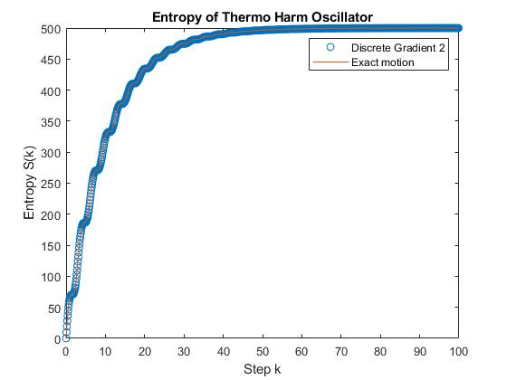
Figure 2: Error of (11): using the same initial data and settings from Figure 1, we plot the error with respect to the exact motion.

5 Conclusions and future work

We have shown the importance of the evolution or horizontal vector field to describe simple thermodynamical systems. We have proven that the restriction of this vector field to constant energy hypersurfaces is a time reparametrization of a Liouville vector field. Also, the relation with the single generation formalism of [EB91a] is elucidated and the construction of geometric integrators satisfying the two laws of thermodynamics.

Of course, our techniques are applied only to simple thermodynamical systems but we consider them to be the building blocks to model more evolved thermodynamical systems using interconnection of these simple systems as in [EMvdS07]. We will study this framework in a future paper.

Moreover, we will study the possibility of introducing the techniques developed in discrete mechanics, in particular, variational integrators, to numerically integrate the equations of the evolution vector field associated to a given Lagrangian function $L:TQ\times\mathbb{R}\longrightarrow\mathbb{R}$. This would allow us to develop higher order methods in a simple way as in [MW01]. In recent papers such as [ASdLLMdD20, VBS19] a discrete Herglotz principle is introduced, allowing to obtain integrators for Lagrangian contact systems. We think that it is possible to adapt the previous constructions to the case of evolution vector fields. We will now develop some of the lines of this future research.

5.1 The geometric setting

Let $L:TQ\times\mathbb{R}\longrightarrow\mathbb{R}$ be a regular Lagrangian function as in Section 3 (see [dLV19, dLV20]). As before, let us introduce coordinates on $TQ\times\mathbb{R}$, denoted by $(q^{i},\dot{q}^{i},S)$, where $(q^{i})$ are coordinates in $Q$, $(q^{i},\dot{q}^{i})$ are the induced bundle coordinates in $TQ$ and $S$ is a global coordinate in $\mathbb{R}$.

Given a Lagrangian function $L$, using the canonical endomorphism ${\mathbf{S}}$ on $TQ$ locally defined by

$${\mathbf{S}}=dq^{i}\otimes\frac{\partial}{\partial\dot{q}^{i}},$$

one can construct a 1-form $\lambda_{L}$ on $TQ\times\mathbb{R}$ given by

$$\lambda_{L}={\mathbf{S}}^{*}(dL)$$

where now ${\mathbf{S}}$ and ${\mathbf{S}}^{*}$ are the natural extensions of ${\mathbf{S}}$ and its adjoint operator ${\mathbf{S}}^{*}$ to $TQ\times\mathbb{R}$ [dRR87].

Therefore, we have that

$$\lambda_{L}=\frac{\partial L}{\partial\dot{q}^{i}}\,dq^{i}.$$

Now, the 1-form on $TQ\times\mathbb{R}$ given by $\eta_{L}=dS-\lambda_{L}$ or, in local coordinates, by

$$\eta_{L}=dS-\frac{\partial L}{\partial\dot{q}^{i}}\,dq^{i}$$

is a contact form on $TQ\times\mathbb{R}$ if and only if $L$ is regular; indeed, if $L$ is regular, then we may prove that $\eta_{L}\wedge(d\eta_{L})^{n}\not=0$, and the converse is also true.

The corresponding Reeb vector field is given in local coordinates by

$${\mathcal{R}}_{L}=\frac{\partial}{\partial S}-W^{ij}\frac{\partial^{2}L}{\partial\dot{q}^{j}\partial S}\,\frac{\partial}{\partial\dot{q}^{i}},$$

where $(W^{ij})$ is the inverse matrix of the Hessian $(W_{ij})$.

The energy of the system is defined by

$$E_{L}=\Delta(L)-L$$

where $\Delta=\dot{q}^{i}\,\frac{\partial}{\partial\dot{q}^{i}}$ is the natural extension of the Liouville vector field on $TQ$ to $TQ\times\mathbb{R}$. Therefore, in local coordinates we have that

$$E_{L}=\dot{q}^{i}\,\frac{\partial L}{\partial\dot{q}^{i}}-L.$$

Denote by $\flat_{L}:T(TQ\times\mathbb{R})\longrightarrow T^{*}(TQ\times\mathbb{R})$ the vector bundle isomorphism given by

$$\flat_{L}(v)=i_{v}(d\eta_{L})+(i_{v}\eta_{L})\,\eta_{L}$$

where $\eta_{L}$ is the contact form on $TQ\times\mathbb{R}$ previously defined. We shall denote its inverse isomorphism by $\sharp_{L}=(\flat_{L})^{-1}$.

Let ${\xi}_{L}$ be the unique vector field satisfying the equation

$$\flat_{L}({\xi}_{L})=dE_{L}-(\mathcal{R}_{L}E_{L}+E_{L})\,\eta_{L}.$$ (12)

A direct computation from eq. (12) shows that if $(q^{i}(t),\dot{q}^{i}(t),S(t))$ is an integral curve of ${\xi}_{L}$, then it satisfies the generalized Euler-Lagrange equations considered by G. Herglotz in 1930:

$$\begin{split}&\frac{d}{dt}\left(\frac{\partial L}{\partial\dot{q}^{i}}\right)-\frac{\partial L}{\partial q^{i}}=\frac{\partial L}{\partial\dot{q}^{i}}\frac{\partial L}{\partial S}\;,\\ &\dot{S}=L(q^{i},\dot{q}^{i},S)\;.\end{split}$$ (13)

Now, given a regular Lagrangian function $L$, we may define the bi-vector $\Lambda_{L}$ on $TQ\times\mathbb{R}$ as in (1) associated to the contact form $\eta_{L}$. That is,

$$\Lambda_{L}(\alpha,\beta)=-d\eta_{L}(\flat_{L}^{-1}(\alpha),\flat_{L}^{-1}(\beta)),\qquad\alpha,\beta\in\Omega^{1}(TQ\times\mathbb{R})\;.$$ (14)

If $(q^{i}(t),\dot{q}^{i}(t),S(t))$ is an integral curve of the evolution vector field ${\mathcal{E}}_{L}$ associated to the contact form $\eta_{L}$ defined by

$${\mathcal{E}}_{L}=\sharp_{\Lambda_{L}}(dE_{L})\hbox{ or }\flat_{L}({\xi}_{L})=dE_{L}-(\mathcal{R}_{L}E_{L})\,\eta_{L}\;,$$

then it satisfies the thermodynamical Herglotz equations

$$\begin{split}&\frac{d}{dt}\left(\frac{\partial L}{\partial\dot{q}^{i}}\right)-\frac{\partial L}{\partial q^{i}}=\frac{\partial L}{\partial\dot{q}^{i}}\frac{\partial L}{\partial S}.\\ &\dot{S}=\dot{q}^{i}\frac{\partial L}{\partial\dot{q}^{i}}.\end{split}$$ (15)

Moreover, if $H$ is the Hamiltonian function defined by $H=E_{L}\circ(\mathbb{F}L)^{-1}$, where $\mathbb{F}L:TQ\times\mathbb{R}\rightarrow T^{*}Q\times\mathbb{R}$ is the Legendre transform, then the evolution vector field ${\mathcal{E}}_{H}$ associated to $H$ is $\mathbb{F}L$-related to ${\mathcal{E}}_{L}$.

5.2 Integration based on discrete Herglotz principle

Now, we propose to construct a numerical integrator for ${\mathcal{E}}_{L}$ based on a similar method to the discrete Herglotz principle [ASdLLMdD20, VBS19].

Let $L_{d}:Q\times Q\times\mathbb{R}\rightarrow\mathbb{R}$ be a discrete Lagrangian function. Then a possible integrator for the evolution dynamics is

$$D_{1}L_{d}(q_{1},q_{2},S_{1})+(1+D_{S}L_{d}((q_{1},q_{2},S_{1}))D_{2}L_{d}(q_{0},q_{1},S_{0})=0$$ (16)

and the entropy is subjected to

$$S_{1}-S_{0}=(q_{1}-q_{0})D_{2}L_{d}(q_{0},q_{1},S_{0}).$$ (17)

Example 3.

Consider again the Hamiltonian function (10) of the damped harmonic oscillator. Since $H$ is regular, we might consider the corresponding Lagrangian function $L:TQ\times\mathbb{R}\rightarrow\mathbb{R}$ given by

$$L(q,\dot{q},S)=\frac{\dot{q}^{2}}{2}-\frac{q^{2}}{2}-\gamma S.$$

A standard discretization of this Lagrangian function is given by means of a quadrature rule like

$$L_{d}(q_{0},q_{1},S_{0})=\frac{(q_{1}-q_{0})^{2}}{2h}-h\frac{(q_{1}+q_{0})^{2}}{8}-h\gamma S_{0}.$$

The discrete Herglotz equations (16) together with (17) give the explicit integrator

$$\begin{split}&q_{2}=\frac{\gamma h^{3}q_{0}+\gamma h^{3}q_{1}+4\gamma hq_{0}-4\gamma hq_{1}-h^{2}q_{0}-2h^{2}q_{1}-4q_{0}+8q_{1}}{h^{2}+4}\\ &S_{1}=S_{0}+\frac{(q_{1}-q_{0})^{2}}{h}-h\frac{q_{1}^{2}-q_{0}^{2}}{4}.\end{split}$$ (18)

In Figures 3 we plot the integrator given by equations (18). We see that the qualitative behaviour of the integrator is also quite good. In fact, an open question is whether the error can be improved by considering discrete Lagrangian functions approximating well enough the exact discrete Lagrangian function.

As a last comment, the entropy for equations (18) is increasing and the Hamiltonian oscillates before stabilizing around a constant value (cf. Fig 4).

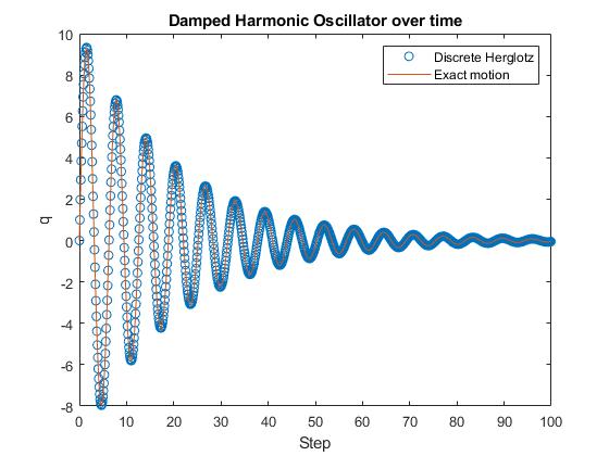
Figure 3: Trajectory of (18): the initial data are $q_{0}=0$, $q_{1}=1$ and $S_{0}=0$; the step is $h=0.1$ and $\gamma=0.1$. We plot the positions $q_{k}$ and compare the integrator with the integral curve of the evolution dynamics ${\mathcal{E}}_{L}$.

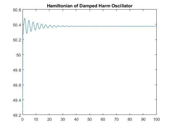
Figure 4: Hamiltonian of (18): using the same initial data and settings from Figure 3, we plot the Hamiltonian function along the iterations of the integrator.

References

• [ASdLLMdD20] Anahory Anahory Simoes, Manuel de León, Manuel Lainz, and David Martín de Diego. On the geometry of discrete contact mechanics. arxiv:2003.11892 [math.ph], 2020.
• [BdLMP20] Alessandro Bravetti, Manuel de León, Juan Carlos Marrero, and Edith Padrón. Contact Hamiltonian systems, Reeb-Liouville dynamics and invariant measures, Preprint, 2020.
• [Bra17] Alessandro Bravetti. Contact Hamiltonian Dynamics: The Concept and Its Use. Entropy, 19(12):535, October 2017.
• [Bra18] Alessandro Bravetti. Contact geometry and thermodynamics. Int. J. Geom. Methods Mod. Phys., 16(supp01):1940003, October 2018.
• [dLLV19] Manuel de León and Manuel Lainz Valcázar. Contact Hamiltonian systems. J. Math. Phys., 60(10):102902, 18, 2019.
• [dLV19] Manuel de León and Manuel Lainz Valcázar. Singular Lagrangians and precontact Hamiltonian Systems. International Journal of Geometric Methods in Modern Physics (forthcoming), August 2019.
• [dLV20] Manuel de León and Manuel Lainz Valcázar. Infinitesimal symmetries in contact hamiltonian systems. Journal of Geometry and Physics, 2020.
• [dRR87] Manuel de León and Paulo R. Rodrigues. Methods of Differential Geometry in Analytical Mechanics, volume 158. Elsevier, Amsterdam, 1987.
• [EB91a] B. J. Edwards and A. N. Beris. Noncanonical Poisson bracket for nonlinear elasticity with extensions to viscoelasticity. J. Phys. A, 24(11):2461–2480, 1991.
• [EB91b] B. J. Edwards and A. N. Beris. Noncanonical Poisson bracket for nonlinear elasticity with extensions to viscoelasticity. J. Phys. A, 24(11):2461–2480, 1991.
• [EMvdS07] Damien Eberard, Bernhard Maschke, and Arjan J. van der Schaft. On the interconnection structures of irreversible physical systems. In Lagrangian and Hamiltonian methods for nonlinear control 2006, volume 366 of Lect. Notes Control Inf. Sci., pages 209–220. Springer, Berlin, 2007.
• [God69] Claude Godbillon. Géométrie différentielle et mécanique analytique. Hermann, Paris, 1969. OCLC: 1038025757.
• [Gon96] O. Gonzalez. Time integration and discrete Hamiltonian systems. J. Nonlinear Sci., 6(5):449–467, 1996.
• [GOR12] Juan Carlos García Orden and Ignacio Romero. Energy-entropy-momentum integration of discrete thermo-visco-elastic dynamics. Eur. J. Mech. A Solids, 32:76–87, 2012.
• [GP20] Sergio Grillo and Edith Padrón. Extended Hamilton-Jacobi theory, contact manifolds, and integrability by quadratures. J. Math. Phys., 61(1):012901, 22, 2020.
• [GY17] François Gay-Balmaz and Hiroaki Yoshimura. A Lagrangian variational formulation for nonequilibrium thermodynamics. Part I: Discrete systems. Journal of Geometry and Physics, 111:169–193, January 2017.
• [GY19] François Gay-Balmaz and Hiroaki Yoshimura. From Lagrangian Mechanics to Nonequilibrium Thermodynamics: A Variational Perspective. Entropy, 21(1):8, January 2019.
• [IA88] T. Itoh and K. Abe. Hamiltonian-conserving discrete canonical equations based on variational difference quotients. J. Comput. Phys., 76(1):85–102, 1988.
• [Kau84] Allan N. Kaufman. Dissipative Hamiltonian systems: a unifying principle. Phys. Lett. A, 100(8):419–422, 1984.
• [LM87] Paulette Libermann and Charles-Michel Marle. Symplectic geometry and analytical mechanics, volume 35 of Mathematics and its Applications. D. Reidel Publishing Co., Dordrecht, 1987. Translated from the French by Bertram Eugene Schwarzbach.
• [Mie11] Alexander Mielke. Formulation of thermoelastic dissipative material behavior using GENERIC. Contin. Mech. Thermodyn., 23(3):233–256, 2011.
• [MNCSS91] Ryszard Mrugala, James D. Nulton, J. Christian Schön, and Peter Salamon. Contact structure in thermodynamic theory. Reports on Mathematical Physics, 29(1):109–121, February 1991.
• [Mor86] Philip J. Morrison. A paradigm for joined Hamiltonian and dissipative systems. volume 18, pages 410–419. 1986. Solitons and coherent structures (Santa Barbara, Calif., 1985).
• [Mru93] R. Mrugala. Continuous contact transformations in thermodynamics. In Proceedings of the XXV Symposium on Mathematical Physics (Toruń, 1992), volume 33, pages 149–154, 1993.
• [MW01] J. E. Marsden and M. West. Discrete mechanics and variational integrators. Acta Numer., 10:357–514, 2001.
• [QT96] G. R. W. Quispel and G. S. Turner. Discrete gradient methods for solving ODEs numerically while preserving a first integral. J. Phys. A, 29(13):L341–L349, 1996.
• [VBS19] Mats Vermeeren, Alessandro Bravetti, and Marcello Seri. Contact variational integrators. J. Phys. A, 52(44):445206, 28, 2019.
• [vdSM19] Arjan van der Schaft and Bernhard Maschke. About some system-theoretic properties of port-thermodynamic systems. In Geometric science of information, volume 11712 of Lecture Notes in Comput. Sci., pages 228–238. Springer, Cham, 2019.