Towards empirical force fields that match experimental observables

Abstract

Biomolecular force fields have been traditionally derived based on a mixture of reference quantum chemistry data and experimental information obtained on small fragments. However, the possibility to run extensive molecular dynamics simulations on larger systems achieving ergodic sampling is paving the way to directly using such simulations along with solution experiments obtained on macromolecular systems. Recently, a number of methods have been introduced to automatize this approach. Here we review these methods, highlight their relationship with machine learning methods, and discuss the open challenges in the field.

I Introduction

Classical molecular dynamics (MD) simulations at the atomistic scale offer a unique opportunity to model the conformational dynamics of biomolecular systems. Being able to reveal mechanisms at spatial and temporal scales that are difficult to observe experimentally, MD simulations are often seen as a computational microscope.Dror et al. (2012) In the past years, they have been applied to study problems ranging from protein folding Lindorff-Larsen et al. (2011) and aggregation Baftizadeh et al. (2012) to RNA-protein interactions,Pérez-Villa, Darvas, and Bussi (2015); Krepl et al. (2015) transmembrane proteins dynamics,Arkhipov et al. (2013) and full viruses,Freddolino et al. (2006) bacteria,Yu et al. (2016) or organelles.Singharoy et al. (2019) The capability of MD simulations to reproduce and predict experimental results is limited by the statistical errors arising from the finite length of simulations and by the systematic errors resulting from the inaccuracies of the underlying models. Interactions are often modeled using empirically parametrized force fields that allow timescales of the order of the microsecond to be routinely simulated. Importantly, the two sources of error mentioned above are deeply intertwined, because only systematic errors that are larger than statistical errors can be detected by comparison with reference experimental results. Indeed, in the past 20 years, the use of special purpose hardware,Shaw et al. (2014) optimized software,Case et al. (2005); Abraham et al. (2015) and enhanced sampling methods,Valsson, Tiwary, and Parrinello (2016); Camilloni and Pietrucci (2018) has significantly reduced the statistical errors, thereby allowing force fields inaccuracies to be detected and largely alleviated. In spite of this, empirical force fields are still far from perfect and in some cases are poorly predictive. For instance, it is not trivial to have force fields capable of simultaneously describing correctly folded, disordered, single-chain proteins or protein complexes,Robustelli, Piana, and Shaw (2018); Piana et al. (2020) to correctly predict RNA structure from sequence-only information across a wide range of structural motifs,Šponer et al. (2018) or to reproduce experimental kinetics in ligand-receptor systems.Capelli et al. (2020)

Solution experiments are optimally suited for validation of force fields, since they provide information about transiently populated structures as well, and they have traditionally been used in this sense. Nevertheless, several approaches have enabled solution experiments to be used directly during force-field fitting, together with available quantum chemistry data. The aim of this perspective is to review these approaches, highlight their relationship with machine learning methods, and discuss the open challenges in the field.

II Empirical force fields: bottom up or top down?

We will use here as paradigmatic examples some of the force fields that are most used for simulating biomolecular systems, namely AMBER,Cornell et al. (1995) CHARMM,MacKerell, Wiorkiewicz-Kuczera, and Karplus (1995) OPLS,Jorgensen and Tirado-Rives (1988) and GROMOS.Oostenbrink et al. (2004) All the mentioned force fields share a common functional form, including bond stretching, angle potentials, torsional potentials, Lennard-Jones, and electrostatic interactions:

$$E=\sum_{bonds}\frac{1}{2}k_{b}(r-r_{0})^{2}+\sum_{angles}\frac{1}{2}k_{a}(a-a_{0})^{2}+\\ \sum_{torsions}\sum_{n}\frac{V_{n}}{2}(1+\cos(n\phi-\delta))+\\ \sum_{LJ}4\epsilon_{ij}\left(\left(\frac{\sigma_{ij}}{r_{ij}}\right)^{12}-\left(\frac{\sigma_{ij}}{r_{ij}}\right)^{6}\right)+\sum_{electrostatics}\frac{q_{i}q_{j}}{r_{ij}}$$ (1)

The parameters ($k_{b};r_{0};k_{a};a_{0};V_{n};\delta;\sigma;\epsilon;q$) are derived from small fragments in advance and depend on the atom type and its chemical environment. Polarizable force fields (such as AMOEBA Shi et al. (2013) and a variant of CHARMM Patel, Mackerell Jr, and Brooks III (2004)), reactive force fields (such as ReaxFF Senftle et al. (2016)), and semi-empirical methods (such as DFTB Seifert and Joswig (2012)) have different functional forms but similar considerations can be applied. The parameters in Eq. 1 are derived with a variety of different procedures that depend on the specific force field and are summarized in Table 1. In particular, some of the parameters are typically derived from quantum chemistry calculations performed at a varying level of accuracy, in a bottom-up spirit. Other parameters are instead derived from experimental data, either using spectroscopy experiments, databases of crystallographic structures, or other gas-phase or solution-phase experiments, in a top-down spirit.

Table 1: Collection of commonly used force fields and method used in their original version for obtaining the respective parameter sets (reference to the original paper is reported for each force field family). A more detailed table is reported in Supplementary Material.

	AMBER Cornell et al. (1995)	CHARMM MacKerell, Wiorkiewicz-Kuczera, and Karplus (1995)	OPLS Jorgensen and Tirado-Rives (1988)	GROMOS Oostenbrink et al. (2004)
Bond	Experiments	Experiments + Ab initio	AMBER parameters	Experiments
Bend	Experiments	Experiments + Ab initio	AMBER parameters	Experiments
Torsion	Experiments + Ab initio	Experiments + Ab initio	AMBER parameters	Ab initio
LJ	Monte Carlo liquid simulations + OPLS parameters	Experiments + Ab initio	Experiments + Ab initio + Monte Carlo liquid simulations	Experiments
Charges	Ab initio	Experiments + Ab initio	Experiments + Ab initio + Monte Carlo liquid simulations	Experiments

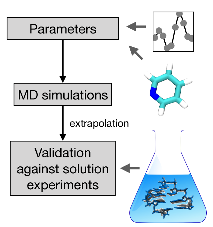
Figure 1: Traditional procedure used for force-field parametrization. Parameters are obtained from calculations or experiments on small molecules or fragments. Simulations are then validated for their capability to maintain the native structure of a macromolecule or against solution experiments. Since fitting and validation are done on different types of systems, there is a large risk associated to extrapolation.

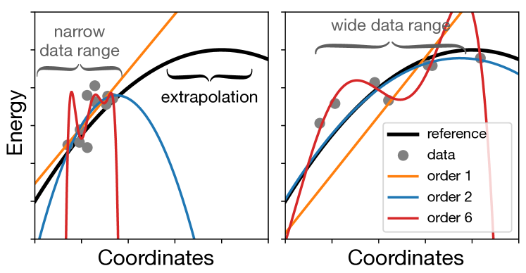
Figure 2: Typical errors observed when fitting a function and extrapolating. The horizontal axis represents a configurational coordinate (e.g., a dihedral angle) and the vertical axis an observable that is used for fitting (e.g., the energy of the system). The true function is shown as a solid line, and the available reference data are shown as grey points. Lines fitted on the reference data using polynomials of increasing order (order 1, 2, and 6) are shown in colors. Data are collected on a narrow (left panel) or wide (right panel) range of configurations. The simple model (order 1) represents a force field with too few parameters or with an incorrect functional form. When fitted on a narrow range of configurations (left panel) it reproduces well the true function. However, it fails the extrapolation to the right part of the graph. When fitted on a wide range of configurations (right panel) the intrinsic limited transferability of the model emerges from the error observed on the fitted points. The complex model (order 2) represents a force field with more parameters and a more physical functional form, since also the reference curve is an order 2 polynomial. When fitted on a narrow range of configurations (left panel) it can lead to significant overfitting. Conversely, when fitted on a wide range of configurations (right panel), it reproduces well the true function on the entire range of configurations. The highest order polynomial (order 6) overfits the reference data in both cases.

One of the factors impacting the reliability of a force field is the accuracy of the employed reference data. For instance, a force field fitted purely on quantum chemistry data cannot provide results that are more accurate than the reference method. However, this limit can be surpassed if multiple sources of data are combined. As an additional and perhaps even more important source of error, one should take into account that reference data used in force-field fitting, either computational or experimental ones, are obtained studying systems that are necessarily not identical to those that one wants to simulate later (see Fig. 1). For instance, torsional parameters and partial charges in the AMBER force field are traditionally obtained using quantum chemistry calculations in small fragments of up to a few dozen atoms, typically including a couple of aminoacids, but are later used to simulate oligopeptides or full protein domains. Similarly, Lennard-Jones parameters in the OPLS force field are obtained from vaporization calorimetry of pure organic liquids such as tetrahydrofuran, pyridine or benzene, but then applied to cases where the analyzed compounds are only portions of a sugar, nucleobase, or aminoacid respectively. These parameters have not been changed in more recent OPLS versions. The reliability of a force field when used in a context different from the one in which it was parametrized depends on the transferability of the functional form in Eq. 1 (see Fig. 2). Given the very large gap between the size and complexity of the systems used for parameter fitting and the systems to which force fields are applied, it appears almost a miracle that current force fields are, for instance, capable of correctly identifying the folded state of a protein.Lindorff-Larsen et al. (2011)

It is interesting to look at a few anecdotal examples to better understand how this is possible. The traditional AMBER force field for nucleic acids has been used for several years before it was realized that sufficiently long simulations could lead to a transition to experimentally unobserved rotamers in the $\alpha$ and $\gamma$ torsions of DNA backbone.Várnai and Zakrzewska (2004); Pérez et al. (2007) Following this empirical observation, a joint effort of several groups lead to the parmbsc0 reparameterization of DNA backbone,Pérez et al. (2007) where the parameters corresponding to these two torsional angles were fitted against quantum chemistry calculations. A similar episode occurred later with the $\chi_{OL3}$ corrections, derived to counteract the occurrence of ladder-like structures in RNA.Zgarbová et al. (2011) In the CHARMM force field for proteins, one of the most important additions after its initial development has been the introduction of empirical corrections maps (CMAP) Mackerell Jr, Feig, and Brooks III (2004), that deviate from the functional form of Eq. 1 by the presence of coupling terms between consecutive torsional angles. These corrections were fitted on quantum chemistry data, but required also a heuristic adjustment to fix the typical values of torsional angles in $\alpha$-helical and $\beta$-sheet regions. As a further example, empirical adjustments of the AMBER and CHARMM force fields were performed respectively in Ref. Best and Hummer, 2009 and in Refs. Piana, Lindorff-Larsen, and Shaw, 2011; Best et al., 2012, where solution data on short oligopeptides were used to optimize backbone dihedrals so as to reproduce helix-coil transitions.

A general trend that can be seen is that experimental data on macromolecular systems (e.g., nucleic acids duplexes or protein domains) are typically used for validation, whereas the parameters are fitted on either theoretical or experimental information available for much smaller systems. Nonetheless, the observation of failures in macromolecular systems is the only way to detect which precise parameters should be corrected. The last three mentioned works, Best and Hummer (2009); Piana, Lindorff-Larsen, and Shaw (2011); Best et al. (2012) instead, report direct fitting of parameters on simulations of short oligomers.

III Recent approaches for fitting force field parameters on experimental data

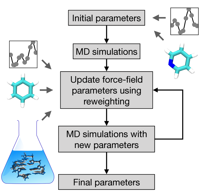
Figure 3: Schematic representation of a force-field fitting procedure using experimental data on macromolecular systems. Initial parameters are tuned based on both quantum chemistry data and experimental data on small systems (e.g., individual residues). Molecular dynamics simulations are then performed on macromolecular systems. Reweighting is used to optimize force field parameters in order to maximize the agreement with a set of available data including experiments on macromolecular systems. In principle, this second stage might include also quantum chemistry data and experimental data on small systems. Even when not explicitly used at this stage, the initial set of quantum chemistry and experimental data is still playing a role for all the parameters that are not further adjusted. Even on the adjusted parameters, the information about the initial force field remains present if regularization terms are included.

A number of approaches have been introduced to allow fitting force fields directly on experimental data taken on macromolecular systems rather than on small fragments, all of them following a flowchart similar to the one illustrated in Fig. 3. Since solution experiments often report results that are averaged over an ensemble of copies of the same molecule, these methods are typically designed to enforce ensemble averages rather than instantaneous values. Norgaard et al. Norgaard, Ferkinghoff-Borg, and Lindorff-Larsen (2008) introduced an approach where a force field is iteratively refined until agreement with experiment is obtained. At each iteration, a simulation is performed and the force field parameters are optimized by assigning new weights to the visited conformations. Thus, through such reweighting procedure, one can predict what result would be obtained using these slightly modified parameters. At some point, when the refined force field and the initial one become too different, it is necessary to iterate the procedure performing a new simulation. The method was applied to the refinement of a coarse-grained model of a protein and fitted against paramagnetic relaxation enhancement experiments. The same method was later used to choose the parameters of an implicit-solvent model against reference all-atom simulations.Bottaro, Lindorff-Larsen, and Best (2013) Li et al. Li and Brüschweiler (2011) showed how to refine an all-atom protein force field using chemical shifts and full-length protein simulations. A common trait of all these methods is that even small changes in force field parameters can make the resulting ensemble very different from the original one making the reweighting procedure less accurate. In Ref. Li and Brüschweiler, 2011, a local reweighting procedure was introduced to alleviate this issue. This procedure is based on the heuristic observation that the ensemble of conformations accessible to a residue is maximally affected by the parameters used for that residue and, to a lesser extent, by the parameters used for the other (possibly identical) residues. Since this is an approximation, a subsequent simulation performed with the corrected force field was necessary to validate the modification. Refs. Wang, Chen, and Van Voorhis, 2012; Wang, Martinez, and Pande, 2014 used a similar automatic procedure to optimize water models. Interestingly, they realized that a straightforward fitting procedure might lead to overfitting and showed how a regularization term can be included in order to alleviate this issue. Finally, Cesari et al. Cesari et al. (2019) introduced a procedure to refine atomistic force fields where heterogenous systems and types of experimental data are used to refine the AMBER RNA force field. Enhanced sampling techniques are employed by the authors to ergodically sample the conformational space for a number of RNA tetramers and hairpin loops, and a regularization term is used in the fitting scheme to maintain the refined force field close to the initial one. The weight of the regularization term is chosen with a cross-validation procedure aimed at maximizing the transferability of the parameters.

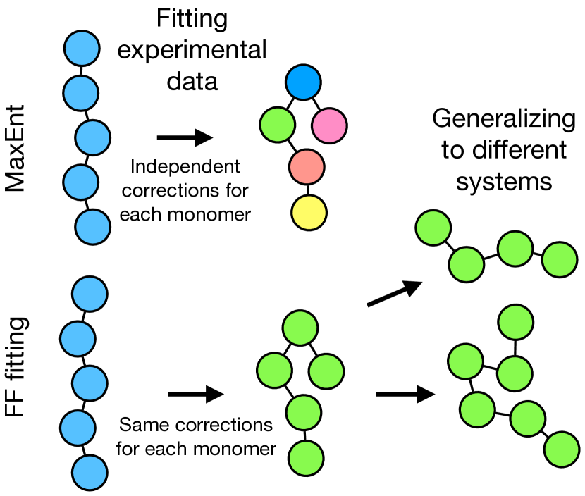
Figure 4: Difference between maximum entropy and force-field fitting procedures. When using the maximum entropy principle to enforce agreement between simulation and experiment, one free parameter is used for each data point. As a consequence, different chemically equivalent units might be treated differently. This does not allow the corrections to be transferred to other molecules, for which new experimental data would be required. When using force-field fitting procedures, instead, all chemically equivalent units are treated in the same manner. This allows the derived parameters to be generalized to other molecules where the same units are used as building blocks.

It is important to recognize the difference between the mentioned approaches, which are meant to generate transferable force-field parameters, and methods meant to improve the agreement with experiment for a specific system for which data are available.Bonomi et al. (2017) This second class includes a variety of approaches such as Bayesian schemesHummer and Köfinger (2015); Bonomi et al. (2016) and methods based on the maximum entropy principle.Pitera and Chodera (2012); Cesari, Reißer, and Bussi (2018) In the maximum entropy formalism the number of free parameters is equal to the number of experimental datapoints. For instance, in a homogenous polymer, each of the monomers will feel a different correction that makes its structure as compatible as possible with experiments. Since the number of parameters is very high, regularization methods can be used and tuned with a cross-validation procedure (see, e.g., Ref. Bottaro et al., 2018). In addition, if a polymer of a different length needs to be simulated, new experimental data should be obtained. In force-field fitting procedures, the chemical structure of the investigated molecule is a priori used to reduce the number of parameters. For instance, in a homogenous polymer, each of the monomers will feel the same correction (although perhaps terminal monomers might be treated differentlyMlỳnskỳ et al. (2020)). On the one hand, this allows to encode a large amount of information in the specific choice of the functional form employed. This type of information is similar to the one that is included when atoms are classified in types in order to obtain their parameters.Mobley et al. (2018) On the other hand, it significantly reduces the number of parameters potentially making the resulting force field transferable. Ref. Cesari, Gil-Ley, and Bussi, 2016 used a hybrid approach were maximum entropy restraints were used but kept by construction constant across chemically equivalent parts of the system. For a recent comparison of approaches taken from both classes, see Ref. Orioli et al., 2020.

Besides the discussed systematic approaches, that report methodological improvements aimed at optimizing parameters based on experimental data, a number of recently developed force fields include terms that were manually adjusted based on the result of MD simulations on systems of different complexity and their capability to reproduce experimental data. For instance, Refs. Robustelli, Piana, and Shaw, 2018; Best and Hummer, 2009; Piana, Lindorff-Larsen, and Shaw, 2011; Best et al., 2012 reported optimizations of parameters based on the solution properties of oligopeptides. The atomic radii of the AMBER ff15ipq force field were chosen so as to provide correct salt-brigde interactions.Debiec et al. (2016) Finally, two recent variants of the AMBER RNA force field contain corrections on hydrogen bonds obtained scanning a series of parameters and minimizing the discrepancy with solution experiment for RNA oligomers.Kührová et al. (2019); Mlỳnskỳ et al. (2020)

IV The machine learning lesson: how to avoid overfitting

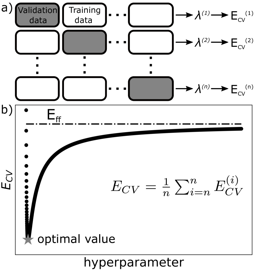
Figure 5: Cross-validation can be used to decrease overfitting and allow more generalizable force-field improvements. a) In $n$-fold cross validation, the data set is randomly split into $n$ blocks of equal size. A single block of data is left out and the parameters are trained on the remaining $n-1$ blocks. This is repeated once for each block, yielding multiple sets of trained parameters $\lambda^{(1)},\dots,\lambda^{(n)}$. The error $E_{CV}^{(k)}$ obtained with parameters $\lambda^{(k)}$ in reproducing the $k$-th block is then computed, and the average over the $n$ results is the cross-validation error ($E_{CV}$). Leave-one-out cross validation is a special case where each block contains a single data point, whereas in leave-$p$-out cross validation all possible subsets of $p$ data are left out. b) Hyperparameters controlling model complexity (such as regularization coefficients) are then chosen so as to minimize the cross-validation error.

Overfitting is a ubiquitous problem when fitting procedures are done in a blind manner. The prototypical cases are machine learning and related algorithms where functions of arbitrary complexity, supported by no or little physical understanding, are used to fit empirical data. The machine learning community has thus developed a number of tools that can be used to avoid or at least alleviate this issue.

Many different machine learning techniques exist and are typically based on a common framework.Mehta et al. (2019) The basic ingredient is a dataset made up of a set of independent variables ($\mathbf{X}$, samples) and a set of dependent variables ($\mathbf{Y}$, labels). Next, a set of models is proposed to map $\mathbf{X}$ into $\mathbf{Y}$ with best accuracy. A model is defined by a set of parameters plus a set of hyperparameters. This splitting is guided by computational convenience such that inference can be approached in a multi-level fashion: typically, model parameters are found by solving an optimization problem at fixed hyperparameters, that on the other hand are preferably scanned over a discrete scale. This double approach is more easily understood when another basic ingredient of machine learning is introduced, that is the cost function. The cost function is used to estimate the performance of a model, and while it is usually a continuous function of the model parameters, it can have a non-trivial dependence on the hyperparameters. For example, the set of hyperparameters can include the architecture of the model, the optimization algorithm used to find the optimal model parameters, the functional form of the cost function itself, etc. Similar choices also need to be taken in force field fitting, as discussed in detail in the next Section.

Since the sets of parameters and hyperparameters defining models are fitted against a finite set of examples $\{\mathbf{X},\mathbf{Y}\}$, overfitting can easily occur. In the limit of fitting on an infinite amount of data, the only limitation of a model would be determined by its complexity. In this limit, a too simple model would underfit the data, leading to a bias in the result. This bias can be decreased by increasing the model complexity. But since in general we deal with datasets of finite size, increasing the complexity of the model would result in a large contribution to the error (variance) due to the sampling. A too complex model would overfit the data, thus having a seriously low performance on new independent data.

The search for the model with the optimal tradeoff between bias and variance (i.e. between under- and over-fitting) follows two directions. One is to split the dataset into a training and a cross-validation set, prior to analysis. Model parameters are fitted against data in the training set, and afterwards the optimized model is validated against the validation set data not included in the training procedure. This procedure is usually referred to as cross-validation (Fig. 5), and depending on how the cross-validation set is built can be referred to as leave-one-out, leave-$p$-out, or $n$-fold cross validation. The other is to reduce the risk of overfitting by means of regularization techniques, the most common consisting in adding terms to the cost function that prevent the model parameters from reaching values extremely adapted to the dataset. This comes at the cost of increasing the number of hyperparameters (e.g., the relative size of training and cross-validation sets, their composition, coefficients of regularization terms, etc.) that continue to be affected by risk of overfitting. Even if a close solution to this problem is not established yet, overfitting should be taken into account for each level of inference (for both parameters and hyperparameters). The most straightforward way to deal with this multi-level risk of overfitting is to a priori split the dataset into three subsets: in addition to the standard training and cross-validation subsets, an independent test set is introduced. The training set is used to fit the optimal values of parameters at fixed hyperparameters; optimal hyperparameters are then fitted against the cross-validation set. Eventually, the performance of the model defined by the optimal parameters and hyperparameters is evaluated on the test set. A more robust approach consists in nested cross-validation Cawley and Talbot (2010), in which parameters and hyperparameters are optimized on a single dataset, but the criterion used to optimize model parameters (training) is different from the optimization criterion used for hyperparameters (model selection). Validation of the selected optimized model against new data that, importantly, has not been used to adjust neither parameters nor hyperparameters, is best practice in this case as well.

V Overfitting in force field development

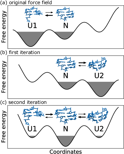
Figure 6: Free-energy landscapes when using reweighting and iterative simulations. The native state, compatible with experimental information, is in the middle (N). Two metastable non-native states that, based on experimental information, are supposed to have a low population, are also shown (U1 and U2). In the original force field (panel a), the N state is sampled, but the most stable state is U1. During the reweighting procedure, the force field learns how to improve the agreement with experiments by disfavoring U1. However, since U2 was never observed in this simulation, there is nothing that prevents it to be stable when using the refined force field. Once a simulation is performed with the refined force field (panel b), the state U2 appears with large population leading to disagreement with experiment. In principle, if a reweighting is performed using only the second simulation, state U1 might appear again with an incorrect population. Only a reweighting where both simulations are combined, and thus all the possible states can be observed, is capable of generating a force field that correctly sets N as the global free-energy minimum and U1 and U2 as metastable states with low population (panel c).

Force-field fitting procedures can be interpreted as machine learning methods where the parameters are the optimized coefficients and data and labels are a mixture of information obtained from both quantum chemistry calculations and various experimental techniques. One should thus pay attention to overfitting. Whenever overfitting occurs, transferability of the force field to a different case might be compromised. As already discussed, if parameters are only fitted on small systems, their transferability to larger systems might be limited. The other phenomenon that can be observed in reweighting methods is the subtle overfitting on the analyzed trajectory. In particular, if parameters are derived to match experimental data by reweighting a trajectory that is not sufficiently long, they might not work correctly on another trajectory obtained using the same force field but with different initial conditions. In addition, since reweighting schemes can only modulate the weight of states that have been explored but cannot predict the population of states that have not been observed (see, e.g., Ref. Rangan et al., 2018 for a comparison of restraining and reweighting when used to implement the maximum entropy principle), the only way to detect these problems is to keep the target force field as close as possible to the original one with some form of regularization and to then perform a new simulation once parameters have been optimized (see Fig. 6).

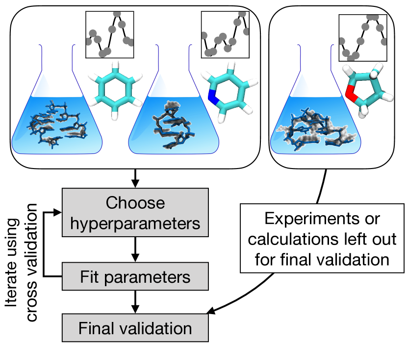
Figure 7: Schematic representation of a training/final-validation procedure. Force-field fitting can be based on a combination of quantum chemistry data, experimental data on small systems and experimental data on macromolecular systems. All data can be used in parameter fitting, and cross-validation (see Fig. 5) can be used to help the choice of hyperparameters. To this end, it is necessary that a separate set of data, either theoretical or experimental, is left out until the very end of the procedure to validate the transferability of the model. This separate data should not be used to take any decision during the fitting procedure, or the information leak might make the final validation not truly independent.

Every other decision taken in the path should be included in the list of hyperparameters. Coefficients controlling regularization terms used in the optimization, that control the relative weight of initial force field and of experimental data, are naturally considered hyperparameters. The functional form of the force field itself is a hyperparameter. The analogous of these hyperparameters in the training of neural network are regularization terms or early stopping criteria and network architecture, respectively.Goodfellow, Bengio, and Courville (2016) In force-field fitting, a number of additional hyperparameters might be used whose control might be more or less explicit. For instance, the so-called forward models used to calculate experimental observables from MD trajectories contain a number of parameters. If the training is done to reproduce the energetics of quantum chemistry calculations, the set of structures used for fitting and their relative weights are to be considered as hyperparameters. Even the precise quantum methods used to compute the total energy might contain a number of hidden parameters (e.g., the possibility to use either implicit or explicit solvent or the specific method used to solve the many-body Schrödinger equation).

If hyperparameters are chosen a priori based on some independent intuition or information, for instance the fact that a given quantum chemistry method is more accurate than another one, then this extra information will be encoded in the final result, improving the quality of the resulting model. However, if hyperparameters are optimized by monitoring the performance of the force field on a specific system, then this system will implicitly become part of the training set. Thus, the resulting model should be validated against a separate system (Fig. 7). A practical example would be if different variants of a force field are derived using three different quantum chemistry methods, then the best method is chosen checking the stability of the native structure of a specific system using all the derived variants. Unless there are other independent evidences that the selected quantum chemistry method is better than the other ones, this choice should be considered as fitted on the specific system and should be then validated on an independent one. Therefore, as a final remark, all the decisions taken in the process should be critically evaluated in this respect.

VI Critical issues and open challenges

The recent works done in adjusting force field parameters including experimental data suggests that this is a promising field that will lead to important improvements in the future. There are however a number of critical issues that one should carefully consider.

First, we suggest that all input data should be considered at the same time, irrespectively of being obtained from experiment or from quantum chemistry calculations. Both experimental and quantum chemistry data can indeed be equivalently used for training or for validation. Importantly, one should consider that different data have different relative errors and different information content. Data that provide limited information during fitting will also provide less stringent validations. Particularly valuable are data obtained on systems as close as possible to those that one is interested in simulating. Less weight instead should be given to data obtained in very different conditions (e.g., without solvent) or on systems that are too simple to be considered as representative (e.g., individual aminoacids or nucleotides). As an exception to this general rule, one should consider that different types of data typically give access to the energetics in different portions of the conformational space. For instance, solution experiments on macromolecular systems are valuable in providing the relative stability of structures that can be distinguished using some probe. Quantum chemistry calculations are instead valuable when states are difficult to be distinguished in the experiment, or when probing rarely visited states (such as transition states).

Reference data should be obtained in conditions as realistic as possible. One should carefully consider the conditions in which experiments are carried out, and prefer experiments performed in conditions that can be reproduced in MD simulations. Ideally, specific experiments might be designed and performed in order to facilitate force field development, such as solution experiments on systems small enough to allow ergodic sampling but large enough to provide transferable information. When instead basing the fits on quantum chemistry calculations, one should consider the importance of the solvent. Additionally, errors in the experimental data should be taken into account. Very important are also errors in the forward models used to connect structures obtained in MD simulations with experiments, since these errors are often larger than the those of the raw data. Errors in the quantum chemistry calculations should be quantified as well.

Taking inspiration from the machine learning community, it is fundamental to understand how to avoid overfitting. In particular, overfitting on specific systems should be avoided, and this can be achieved by including as heterogenous as possible systems in the dataset. Similarly, overfitting should be avoided on specific trajectories. To this end, separate validation simulations can be run or robust estimates of the statistical errors can be pursued. Regularization terms can be used to tune model complexity thus reducing the impact of overfitting. Validation should be made on data that are obtained in an as independent as possible manner.

Finally, the current functional form (Eq. 1) might be too limited to be usable on a wide range of cases. Increasing the complexity of the model might help in this respect. Complexity can be introduced by physical insight (e.g., explicitly polarizable force fields Patel, Mackerell Jr, and Brooks III (2004); Shi et al. (2013) or modified Lennard-Jones potentials Li and Merz Jr (2014)) or by blind learning of non-linear models (e.g., neural network potentials Behler and Parrinello (2007); Smith, Isayev, and Roitberg (2017)). Nonetheless, one should keep in mind that, whenever complexity is increased, overfitting has more chance to appear. In this respect, for a fixed number of parameters, the more physical the functional form is, the less it will tend to overfit. Interestingly, neural networks are now routinely used to fit bottom up potentials where the training data can be generated by computational methods and can then be easily made very abundant.Behler and Parrinello (2007); Smith, Isayev, and Roitberg (2017); Noé et al. (2020); Gkeka et al. (2020) These approaches are however typically designed to be trained on very small systems or chemical groups, and their applicability to macromolecular systems has not been shown yet. It is thus still to be seen if neural network potentials can be used fruitfully when force fields are directly fitted on experimental data.

Supplementary Material

A table reporting more details about the methods used to obtain parameters in the most common biomolecular force field.

Data availability

Data sharing not applicable — no new data generated.

References

- Dror et al. (2012) R. O. Dror, R. M. Dirks, J. Grossman, H. Xu, and D. E. Shaw, “Biomolecular simulation: a computational microscope for molecular biology,” Annu. Rev. Biophys. 41, 429–452 (2012).
- Lindorff-Larsen et al. (2011) K. Lindorff-Larsen, S. Piana, R. O. Dror, and D. E. Shaw, “How fast-folding proteins fold,” Science 334, 517–520 (2011).
- Baftizadeh et al. (2012) F. Baftizadeh, X. Biarnes, F. Pietrucci, F. Affinito, and A. Laio, “Multidimensional view of amyloid fibril nucleation in atomistic detail,” J. Am. Chem. Soc. 134, 3886–3894 (2012).
- Pérez-Villa, Darvas, and Bussi (2015) A. Pérez-Villa, M. Darvas, and G. Bussi, “ATP dependent NS3 helicase interaction with RNA: insights from molecular simulations,” Nucleic Acids Res. 43, 8725–8734 (2015).
- Krepl et al. (2015) M. Krepl, M. Havrila, P. Stadlbauer, P. Banáš, M. Otyepka, J. Pasulka, R. Stefl, and J. Šponer, “Can we execute stable microsecond-scale atomistic simulations of protein–RNA complexes?” J. Chem. Theory Comput. 11, 1220–1243 (2015).
- Arkhipov et al. (2013) A. Arkhipov, Y. Shan, R. Das, N. F. Endres, M. P. Eastwood, D. E. Wemmer, J. Kuriyan, and D. E. Shaw, “Architecture and membrane interactions of the EGF receptor,” Cell 152, 557–569 (2013).
- Freddolino et al. (2006) P. L. Freddolino, A. S. Arkhipov, S. B. Larson, A. McPherson, and K. Schulten, “Molecular dynamics simulations of the complete satellite tobacco mosaic virus,” Structure 14, 437–449 (2006).
- Yu et al. (2016) I. Yu, T. Mori, T. Ando, R. Harada, J. Jung, Y. Sugita, and M. Feig, “Biomolecular interactions modulate macromolecular structure and dynamics in atomistic model of a bacterial cytoplasm,” Elife 5, e19274 (2016).
- Singharoy et al. (2019) A. Singharoy, C. Maffeo, K. H. Delgado-Magnero, D. J. Swainsbury, M. Sener, U. Kleinekathöfer, J. W. Vant, J. Nguyen, A. Hitchcock, B. Isralewitz, et al., “Atoms to phenotypes: Molecular design principles of cellular energy metabolism,” Cell 179, 1098–1111 (2019).
- Shaw et al. (2014) D. E. Shaw, J. Grossman, J. A. Bank, B. Batson, J. A. Butts, J. C. Chao, M. M. Deneroff, R. O. Dror, A. Even, C. H. Fenton, et al., “Anton 2: raising the bar for performance and programmability in a special-purpose molecular dynamics supercomputer,” in SC’14: Proceedings of the International Conference for High Performance Computing, Networking, Storage and Analysis (IEEE, 2014) pp. 41–53.
- Case et al. (2005) D. A. Case, T. E. Cheatham III, T. Darden, H. Gohlke, R. Luo, K. M. Merz Jr, A. Onufriev, C. Simmerling, B. Wang, and R. J. Woods, “The Amber biomolecular simulation programs,” J. Comput. Chem. 26, 1668–1688 (2005).
- Abraham et al. (2015) M. J. Abraham, T. Murtola, R. Schulz, S. Páll, J. C. Smith, B. Hess, and E. Lindahl, “GROMACS: High performance molecular simulations through multi-level parallelism from laptops to supercomputers,” SoftwareX 1, 19–25 (2015).
- Valsson, Tiwary, and Parrinello (2016) O. Valsson, P. Tiwary, and M. Parrinello, “Enhancing important fluctuations: Rare events and metadynamics from a conceptual viewpoint,” Annu. Rev. Phys. Chem. 67, 159–184 (2016).
- Camilloni and Pietrucci (2018) C. Camilloni and F. Pietrucci, “Advanced simulation techniques for the thermodynamic and kinetic characterization of biological systems,” Adv. Phys. X 3, 1477531 (2018).
- Robustelli, Piana, and Shaw (2018) P. Robustelli, S. Piana, and D. E. Shaw, “Developing a molecular dynamics force field for both folded and disordered protein states,” Proc. Natl. Acad. Sci. U.S.A. 115, E4758–E4766 (2018).
- Piana et al. (2020) S. Piana, P. Robustelli, D. Tan, S. Chen, and D. E. Shaw, “Development of a force field for the simulation of single-chain proteins and protein-protein complexes,” J. Chem. Theory Comput. 16, 2494–2507 (2020).
- Šponer et al. (2018) J. Šponer, G. Bussi, M. Krepl, P. Banáš, S. Bottaro, R. A. Cunha, A. Gil-Ley, G. Pinamonti, S. Poblete, P. Jurečka, N. G. Walter, and M. Otyepka, “RNA structural dynamics as captured by molecular simulations: a comprehensive overview,” Chem. Rev. 118, 4177–4338 (2018).
- Capelli et al. (2020) R. Capelli, W. Lyu, V. Bolnykh, S. Meloni, J. M. H. Olsen, U. Rothlisberger, M. Parrinello, and P. Carloni, “On the accuracy of molecular simulation-based predictions of koff values: a metadynamics study,” bioRxiv preprint, doi:10.1101/2020.03.30.015396 (2020).
- Cornell et al. (1995) W. D. Cornell, P. Cieplak, C. I. Bayly, I. R. Gould, K. M. Merz, D. M. Ferguson, D. C. Spellmeyer, T. Fox, J. W. Caldwell, and P. A. Kollman, “A second generation force field for the simulation of proteins, nucleic acids, and organic molecules,” J. Am. Chem. Soc. 117, 5179–5197 (1995).
- MacKerell, Wiorkiewicz-Kuczera, and Karplus (1995) A. D. MacKerell, J. Wiorkiewicz-Kuczera, and M. Karplus, “An all-atom empirical energy function for the simulation of nucleic acids,” J. Am. Chem. Soc. 117, 11946–11975 (1995).
- Jorgensen and Tirado-Rives (1988) W. L. Jorgensen and J. Tirado-Rives, “The OPLS [optimized potentials for liquid simulations] potential functions for proteins, energy minimizations for crystals of cyclic peptides and crambin,” J. Am. Chem. Soc. 110, 1657–1666 (1988).
- Oostenbrink et al. (2004) C. Oostenbrink, A. Villa, A. E. Mark, and W. F. Van Gunsteren, “A biomolecular force field based on the free enthalpy of hydration and solvation: The GROMOS force-field parameter sets 53A5 and 53A6,” J. Comput. Chem. 25, 1656–1676 (2004).
- Shi et al. (2013) Y. Shi, Z. Xia, J. Zhang, R. Best, C. Wu, J. W. Ponder, and P. Ren, “Polarizable atomic multipole-based AMOEBA force field for proteins,” J. Chem. Theory Comput. 9, 4046–4063 (2013).
- Patel, Mackerell Jr, and Brooks III (2004) S. Patel, A. D. Mackerell Jr, and C. L. Brooks III, “CHARMM fluctuating charge force field for proteins: II protein/solvent properties from molecular dynamics simulations using a nonadditive electrostatic model,” J. Comput. Chem. 25, 1504–1514 (2004).
- Senftle et al. (2016) T. P. Senftle, S. Hong, M. M. Islam, S. B. Kylasa, Y. Zheng, Y. K. Shin, C. Junkermeier, R. Engel-Herbert, M. J. Janik, H. M. Aktulga, et al., “The ReaxFF reactive force-field: development, applications and future directions,” NPJ Comput. Mater. 2, 1–14 (2016).
- Seifert and Joswig (2012) G. Seifert and J.-O. Joswig, “Density-functional tight binding – an approximate density-functional theory method,” Wiley Interdiscip. Rev. Comput. Mol. Sci. 2, 456–465 (2012).
- Várnai and Zakrzewska (2004) P. Várnai and K. Zakrzewska, “DNA and its counterions: a molecular dynamics study,” Nucleic Acids Res. 32, 4269–4280 (2004).
- Pérez et al. (2007) A. Pérez, I. Marchán, D. Svozil, J. Šponer, T. E. Cheatham III, C. A. Laughton, and M. Orozco, “Refinement of the AMBER force field for nucleic acids: improving the description of / conformers,” Biophys. J. 92, 3817–3829 (2007).
- Zgarbová et al. (2011) M. Zgarbová, M. Otyepka, J. Šponer, A. Mládek, P. Banáš, T. E. Cheatham, and P. Jurečka, “Refinement of the Cornell et al. nucleic acids force field based on reference quantum chemical calculations of glycosidic torsion profiles,” J. Chem. Theory Comput. 7, 2886–2902 (2011).
- Mackerell Jr, Feig, and Brooks III (2004) A. D. Mackerell Jr, M. Feig, and C. L. Brooks III, “Extending the treatment of backbone energetics in protein force fields: limitations of gas-phase quantum mechanics in reproducing protein conformational distributions in molecular dynamics simulations,” J. Comput. Chem. 25, 1400–1415 (2004).
- Best and Hummer (2009) R. B. Best and G. Hummer, “Optimized molecular dynamics force fields applied to the helix-coil transition of polypeptides,” J. Phys. Chem. B 113, 9004–9015 (2009).
- Piana, Lindorff-Larsen, and Shaw (2011) S. Piana, K. Lindorff-Larsen, and D. E. Shaw, “How robust are protein folding simulations with respect to force field parameterization?” Biophys. J. 100, L47–L49 (2011).
- Best et al. (2012) R. B. Best, X. Zhu, J. Shim, P. E. Lopes, J. Mittal, M. Feig, and A. D. MacKerell Jr, “Optimization of the additive CHARMM all-atom protein force field targeting improved sampling of the backbone , and side-chain 1 and 2 dihedral angles,” J. Chem Theory Comput. 8, 3257–3273 (2012).
- Norgaard, Ferkinghoff-Borg, and Lindorff-Larsen (2008) A. B. Norgaard, J. Ferkinghoff-Borg, and K. Lindorff-Larsen, “Experimental parameterization of an energy function for the simulation of unfolded proteins,” Biophys. J. 94, 182–192 (2008).
- Bottaro, Lindorff-Larsen, and Best (2013) S. Bottaro, K. Lindorff-Larsen, and R. B. Best, “Variational optimization of an all-atom implicit solvent force field to match explicit solvent simulation data,” J. Chem Theory Comput. 9, 5641–5652 (2013).
- Li and Brüschweiler (2011) D.-W. Li and R. Brüschweiler, “Iterative optimization of molecular mechanics force fields from NMR data of full-length proteins,” J. Chem. Theory Comput. 7, 1773–1782 (2011).
- Wang, Chen, and Van Voorhis (2012) L.-P. Wang, J. Chen, and T. Van Voorhis, “Systematic parametrization of polarizable force fields from quantum chemistry data,” J. Chem. Theory Comput. 9, 452–460 (2012).
- Wang, Martinez, and Pande (2014) L.-P. Wang, T. J. Martinez, and V. S. Pande, “Building force fields: an automatic, systematic, and reproducible approach,” J. Phys. Chem. Lett. 5, 1885–1891 (2014).
- Cesari et al. (2019) A. Cesari, S. Bottaro, K. Lindorff-Larsen, P. Banáš, J. Šponer, and G. Bussi, “Fitting corrections to an RNA force field using experimental data,” J. Chem. Theory Comput. 15, 3425–3431 (2019).
- Bonomi et al. (2017) M. Bonomi, G. T. Heller, C. Camilloni, and M. Vendruscolo, “Principles of protein structural ensemble determination,” Curr. Opin. Struct. Biol. 42, 106–116 (2017).
- Hummer and Köfinger (2015) G. Hummer and J. Köfinger, “Bayesian ensemble refinement by replica simulations and reweighting,” J. Chem. Phys. 143, 12B634_1 (2015).
- Bonomi et al. (2016) M. Bonomi, C. Camilloni, A. Cavalli, and M. Vendruscolo, “Metainference: A Bayesian inference method for heterogeneous systems,” Sci. Adv. 2, e1501177 (2016).
- Pitera and Chodera (2012) J. W. Pitera and J. D. Chodera, “On the use of experimental observations to bias simulated ensembles,” J. Chem. Theory Comput. 8, 3445–3451 (2012).
- Cesari, Reißer, and Bussi (2018) A. Cesari, S. Reißer, and G. Bussi, “Using the maximum entropy principle to combine simulations and solution experiments,” Computation 6, 15 (2018).
- Bottaro et al. (2018) S. Bottaro, G. Bussi, S. D. Kennedy, D. H. Turner, and K. Lindorff-Larsen, “Conformational ensembles of RNA oligonucleotides from integrating NMR and molecular simulations,” Science Adv. 4, eaar8521 (2018).
- Mlỳnskỳ et al. (2020) V. Mlỳnskỳ, P. Kührová, T. Kühr, M. Otyepka, G. Bussi, P. Banáš, and J. Šponer, “Fine-tuning of the AMBER RNA force field with a new term adjusting interactions of terminal nucleotides,” J. Chem. Theory Comput., doi:10.1021/acs.jctc.0c00228 (2020).
- Mobley et al. (2018) D. L. Mobley, C. C. Bannan, A. Rizzi, C. I. Bayly, J. D. Chodera, V. T. Lim, N. M. Lim, K. A. Beauchamp, D. R. Slochower, M. R. Shirts, et al., “Escaping atom types in force fields using direct chemical perception,” J. Chem. Theory Comput. 14, 6076–6092 (2018).
- Cesari, Gil-Ley, and Bussi (2016) A. Cesari, A. Gil-Ley, and G. Bussi, “Combining simulations and solution experiments as a paradigm for RNA force field refinement,” J. Chem. Theory Comput. 12, 6192–6200 (2016).
- Orioli et al. (2020) S. Orioli, A. H. Larsen, S. Bottaro, and K. Lindorff-Larsen, “How to learn from inconsistencies: Integrating molecular simulations with experimental data,” Prog. Mol. Biol. Transl. 170, 123–176 (2020).
- Debiec et al. (2016) K. T. Debiec, D. S. Cerutti, L. R. Baker, A. M. Gronenborn, D. A. Case, and L. T. Chong, “Further along the road less traveled: AMBER ff15ipq, an original protein force field built on a self-consistent physical model,” J. Chem. Theory Comput. 12, 3926–3947 (2016).
- Kührová et al. (2019) P. Kührová, V. Mlỳnskỳ, M. Zgarbová, M. Krepl, G. Bussi, R. B. Best, M. Otyepka, J. Šponer, and P. Banáš, “Improving the performance of the AMBER RNA force field by tuning the hydrogen-bonding interactions,” J. Chem. Theory Comput. 15, 3288–3305 (2019).
- Mehta et al. (2019) P. Mehta, M. Bukov, C.-H. Wang, A. G. Day, C. Richardson, C. K. Fisher, and D. J. Schwab, “A high-bias, low-variance introduction to machine learning for physicists,” Phys. Rep. 810, 1–124 (2019).
- Cawley and Talbot (2010) G. C. Cawley and N. L. Talbot, “On over-fitting in model selection and subsequent selection bias in performance evaluation,” J. Mach. Learn. Res. 11, 2079–2107 (2010).
- Rangan et al. (2018) R. Rangan, M. Bonomi, G. T. Heller, A. Cesari, G. Bussi, and M. Vendruscolo, “Determination of structural ensembles of proteins: restraining vs reweighting,” J. Chem. Theory Comput. 14, 6632–6641 (2018).
- Goodfellow, Bengio, and Courville (2016) I. Goodfellow, Y. Bengio, and A. Courville, Deep learning (MIT press, 2016).
- Li and Merz Jr (2014) P. Li and K. M. Merz Jr, “Taking into account the ion-induced dipole interaction in the nonbonded model of ions,” J. Chem Theory Comput. 10, 289–297 (2014).
- Behler and Parrinello (2007) J. Behler and M. Parrinello, “Generalized neural-network representation of high-dimensional potential-energy surfaces,” Phys. Rev. Lett. 98, 146401 (2007).
- Smith, Isayev, and Roitberg (2017) J. S. Smith, O. Isayev, and A. E. Roitberg, “ANI-1: an extensible neural network potential with DFT accuracy at force field computational cost,” Chem. Sci. 8, 3192–3203 (2017).
- Noé et al. (2020) F. Noé, A. Tkatchenko, K.-R. Müller, and C. Clementi, “Machine learning for molecular simulation,” Annu. Rev. Phys. Chem. 71, doi: 10.1146/annurev–physchem–042018–052331 (2020).
- Gkeka et al. (2020) P. Gkeka, G. Stoltz, A. B. Farimani, Z. Belkacemi, M. Ceriotti, J. Chodera, A. R. Dinner, A. Ferguson, J.-B. Maillet, H. Minoux, et al., “Machine learning force fields and coarse-grained variables in molecular dynamics: application to materials and biological systems,” arXiv preprint arXiv:2004.06950 (2020).