Towards a Parallel-in-Time Calculation of Time-Periodic Solutions with Unknown Period

Abstract

This paper presents a novel parallel-in-time algorithm able to compute time-periodic solutions of problems where the period is not given. Exploiting the idea of the multiple shooting method, the proposed approach calculates the initial values at each subinterval as well as the corresponding period iteratively. As in the Parareal method, parallelization in the time domain is performed using discretization on a two-level grid. A special linearization of the time-periodic system on the coarse grid is introduced to speed up the computations. The iterative algorithm is verified via its application to the Colpitts oscillator model.

1 Introduction

Steady-state analysis is a common task in electrical engineering, for example, during the initial design stages of, e.g., electric circuits or motors. Classical sequential time stepping may lead to lengthy transient computation particularly when the underlying dynamical system possesses a large time constant. Various approaches for efficient steady-state calculation are known from the literature. For instance, clever methods to choose the starting value Bermudez_2019aa or an explicit error correction Takahashi_2010aa could accelerate the time-domain calculation considerably.

A powerful tool for speeding up the classical time stepping is the class of parallel-in-time methods, such as the multigrid reduction in time Falgout_2014aa or Parareal Lions_2001aa . Originating from the multiple shooting method Morrison_1962aa , they are based on the splitting of the considered time interval into several windows and updating the solution at synchronization points iteratively. The use of coarse and fine discretizations propagates quickly low-frequency information of the solution using a cheap sequential solver followed by a very accurate result with a precise fine solver applied in parallel.

Another direction of obtaining the steady state is based on the solution of the joint space- and time-discrete time-periodic system formulated on the whole period Hara_1985aa . There the initial and final values are coupled through the prescribed periodicity condition. An obstacle within the solution of the periodic problem in the time domain becomes the large size of the system matrix as well as its special block structure due to the interdependence of the solution vectors over the period. To deal with this difficulty a frequency domain approach was proposed in Biro_2006aa . In case of linear problems, the method takes advantage of the block-cyclic matrix structure by applying the discrete Fourier transform. It fully decouples the variables, thereby allowing for the separate solution of each harmonic coefficient. This approach was further extended and incorporated into the Parareal framework by the authors in Kulchytska-Ruchka_2019ag . There, a simplified Newton-based iterative algorithm was presented together with its convergence analysis for the efficient treatment of nonlinear problems.

Solutions of time-periodic problems become much more challenging when the period is not given. Such situation occurs, e.g., when dealing with an autonomous system Deuflhard_1984aa . In contrast to a non-autonomous problem, the periodicity cannot be determined from the applied excitation. This paper proposes a numerical algorithm capable of determining an appropriate period automatically using parallelization in the time domain. Extending the idea of the multiple shooting method we include the unknown period together with multiple initial values as the sought parameters into the iterative procedure. Verification of the presented approach is illustrated through its application to the Colpitts oscillator model Kampowsky_1992aa .

The paper is organized as follows. Section 2 describes the basis of the multiple shooting approach including the unknown period as an additional variable. This is further expanded to the family of the Parareal-based methods in Section 3. Section 4 applies the proposed parallel-in-time approach to the Colpitts oscillator model using a particular linerization on the coarse level. The paper is finally summarized in Section 5.

2 Multiple shooting with unknown period

We consider the following time-periodic problem for a system of ordinary differential equations (ODEs)

$$\mathbf{M}\tilde{\mathbf{u}}^{\prime}(t) =\mathbf{f}(\tilde{\mathbf{u}}(t)),\ \ t\in(0,T)$$ (1)

$$\tilde{\mathbf{u}}(0) =\tilde{\mathbf{u}}(T),$$

where the period $T>0$ and the vector $\tilde{\mathbf{u}}:[0,T]\to\mathbb{R}^{d},$ $d\geq 1$ are sought. $\mathbf{M}$ is a given non-singular mass matrix, $\mathbf{f}$ is a bounded and Lipschitz continous right-hand side (RHS) function. Following Deuflhard_1984aa we incorporate the period $T$ as an unknown parameter by performing the change of variables

$$[0,T]\ni t\mapsto\tau:=t/T\in[0,1].$$ (2)

The problem (1) is thereby transformed into the equivalent one: find $T>0$ and ${\mathbf{u}}:[0,1]\to\mathbb{R}^{d}$ such that

$$\mathbf{M}{\mathbf{u}}^{\prime}(\tau) =T\mathbf{f}({\mathbf{u}}(\tau)),\ \ \tau\in(0,1)$$ (3)

$${\mathbf{u}}(0) ={\mathbf{u}}(1).$$

The unit interval $[0,1]$ is then partitioned into $N$ windows by the nodes $0=\tau_{0}<\tau_{1}<\dots<\tau_{N}=1.$ The $n$-th subinterval has length $\Delta\tau_{n}=\tau_{n}-\tau_{n-1},$ for $n=1,\dots,N.$

For a given discrete variable $\mathbf{U}_{n-1}$, we consider an initial value problem (IVP) on the window $(\tau_{n-1},\tau_{n}]$

$$\mathbf{M}{\mathbf{u}}^{\prime}_{n}(\tau) =T\mathbf{f}({\mathbf{u}_{n}}(\tau)),\ \ \tau\in(\tau_{n-1},\tau_{n}]$$ (4)

$${\mathbf{u}_{n}}(\tau_{n-1}) ={\mathbf{U}_{n-1}}$$

and let $\mathcal{F}(\tau_{n},\tau_{n-1},\mathbf{U}_{n-1},T)$ denote the solution operator of (4) for $n=1,\dots,N.$ A sketch of the piecewise-defined solution due to the interval splitting is shown in Fig. 1. In order to eliminate the jumps at the synchronization points $\tau_{n},$ $n=1,\dots,N-1$ as well as the difference between the initial value at $\tau_{0}$ and the final one at $\tau_{N}$ the matching conditions:

$$\varPhi(\mathbf{z}):=\left\{\begin{aligned} \mathcal{F}(\tau_{N},\tau_{N-1},\mathbf{U}_{N-1},T)-\mathbf{U}_{0}&=0,\\ \mathcal{F}(\tau_{n},\tau_{n-1},\mathbf{U}_{n-1},T)-\mathbf{U}_{n}&=0,\ \ n=1,\dots,N-1\end{aligned}\right.$$ (5)

have to be satisfied, where $\mathbf{z}=\left[\mathbf{U}_{0}^{\top},\dots,\mathbf{U}_{N-1}^{\top},T\right]^{\!\top}\!.$ System (5) represents the root-finding problem for the mapping $\varPhi:\mathbb{R}^{Nd+1}\rightarrow\mathbb{R}^{Nd}.$ The Jacobian of $\varPhi$ is given by

$$\mathbf{J}_{\varPhi}(\mathbf{z})=\begin{bmatrix}-\mathbf{I}&&&\mathbf{G}_{N}&\mathbf{g}_{N}\\ \mathbf{G}_{1}&-\mathbf{I}&&&\mathbf{g}_{1}\\ &\ddots&\ddots&&\vdots\\ &&\mathbf{G}_{N-1}&-\mathbf{I}&\mathbf{g}_{N-1}\end{bmatrix},$$ (6)

where

$$\mathbf{G}_{n}=\frac{\partial\mathcal{F}}{\partial\mathbf{U}_{n-1}}(\tau_{n},\tau_{n-1},\mathbf{U}_{n-1},T),\qquad\mathbf{g}_{n}=\frac{\partial\mathcal{F}}{\partial T}(\tau_{n},\tau_{n-1},\mathbf{U}_{n-1},T),$$ (7)

$n=1,\dots,N$ and $\mathbf{I}$ is the identity matrix. The root $\mathbf{z}$ of (5) can then be calculated using the Newton method, i.e., for a given $\mathbf{z}^{(0)}$ and $k=0,1,\dots$ solution $\mathbf{z}^{(k+1)}$ at the iteration $k+1$ is updated through

$$\mathbf{J}_{\varPhi}\bigl{(}\mathbf{z}^{(k)}\bigr{)}\Delta\mathbf{z}^{(k)} =-{\varPhi}\bigl{(}\mathbf{z}^{(k)}\bigr{)},$$ (8)

$$\mathbf{z}^{(k+1)} =\Delta\mathbf{z}^{(k)}+\mathbf{z}^{(k)}.$$ (9)

Note that due to the introduction of the additional variable $T$ the system of equations (8) is underdetermined and can be solved, e.g., by calculating the Moore-Penrose pseudoinverse. A generalized eigenvalue-based gauging as well as the corresponding theory for the Moore-Penrose pseudoinversion was presented in Boroujeni_2010aa . We note that in case when the size of (8) is large it can be condensed to a $d$-dimensional system with $d+1$ unknowns by block Gaussian elimination Deuflhard_1984aa .

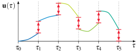
Figure 1: Example of the interval splitting within the multiple shooting for $N=5$. The mismatches at the synchronization points $\tau_{n},$ $n=1,\dots,N-1$ together with the periodicity jump between the solution at $\tau_{0}$ and $\tau_{N}$ are eliminated (up to a prescribed tolerance) by solving the root-finding problem.

3 Periodic time-parallelization with coarse grid correction

Inheriting the idea of the Parareal algorithm Lions_2001aa ; Gander_2007ab we approximate the derivative in $\mathbf{G}_{n}$ (7) in a finite difference way using a coarse propagator $\mathcal{G},$ i.e., for the iteration $k$ and $n=1,\dots,N$

$$\mathbf{G}_{n}^{(k)}\Delta\mathbf{U}_{n-1}^{(k)} =\frac{\partial\mathcal{F}}{\partial\mathbf{U}_{n-1}}\bigl{(}\tau_{n},\tau_{n-1},\mathbf{U}_{n-1}^{(k)},T\bigr{)}\bigl{[}\mathbf{U}_{n-1}^{(k+1)}-\mathbf{U}_{n-1}^{(k)}\bigr{]}$$ (10)

$$\approx\mathcal{G}\bigl{(}\tau_{n},\tau_{n-1},\mathbf{U}_{n-1}^{(k+1)},T\bigr{)}-\mathcal{G}\bigl{(}\tau_{n},\tau_{n-1},\mathbf{U}_{n-1}^{(k)},T\bigr{)}.$$

Similar to the fine propagator $\mathcal{F},$ the operator $\mathcal{G}$ solves the IVP (4) on each time window. However, in contrast to the fine solver the coarse propagator has a considerably lower precision, e.g., it uses a lower-order time integrator or bigger time steps. Substituting (10) into (8) we obtain the periodic Parareal with periodic coarse problem Gander_2013ab with unknown period (PP-PC-UP):

$$\begin{bmatrix}-\mathbf{I}&&&{\mathcal{G}_{N}\left(\cdot,T\right)}&\mathbf{g}^{(k)}_{N}\\ {\mathcal{G}_{1}\left(\cdot,T\right)}&-\mathbf{I}&&&\mathbf{g}^{(k)}_{1}\\ &\ddots&\ddots&&\vdots\\ &&{\mathcal{G}_{N-1}\left(\cdot,T\right)}&-\mathbf{I}&\mathbf{g}^{(k)}_{N-1}\end{bmatrix}\begin{bmatrix}\mathbf{U}_{0}^{(k+1)}\\ \mathbf{U}_{1}^{(k+1)}\\ \vdots\\ \mathbf{U}_{N-1}^{(k+1)}\\ T^{(k+1)}\end{bmatrix}=\begin{bmatrix}\mathbf{b}_{N}^{(k)}\\ \mathbf{b}_{1}^{(k)}\\ \vdots\\ \mathbf{b}_{N-1}^{(k)}\end{bmatrix},$$ (11)

where we denote $\mathbf{b}_{n}^{(k)}:=\mathbf{g}_{n}^{(k)}T^{(k)}+\mathcal{G}\bigl{(}\tau_{n},\tau_{n-1},\mathbf{U}^{(k)}_{n-1},T\bigr{)}-\mathcal{F}\bigl{(}\tau_{n},\tau_{n-1},\mathbf{U}^{(k)}_{n-1},T\bigr{)}$ and $\mathcal{G}_{n}\bigl{(}\cdot,T\bigr{)}:=\mathcal{G}\bigl{(}\tau_{n},\tau_{n-1},\cdot,T\bigr{)}$ for $n=1,\dots,N.$ Following Deuflhard_1984aa we have

$$\mathbf{g}_{n}^{(k)} =\frac{\partial\mathcal{F}}{\partial T}\bigl{(}\tau_{n},\tau_{n-1},\mathbf{U}_{n-1}^{(k)},T\bigr{)}=\frac{\partial}{\partial T}\Bigl{[}\mathbf{U}_{n-1}^{(k)}+\mathbf{M}^{-1}\int\limits_{\tau_{n-1}}^{\tau_{n}}T\mathbf{f}({\mathbf{u}}(\tau))d\tau\Bigr{]}$$ (12)

$$=\mathbf{M}^{-1}\int\limits_{\tau_{n-1}}^{\tau_{n}}\mathbf{f}({\mathbf{u}}(\tau))d\tau\approx\mathbf{M}^{-1}\Delta\tau_{n}\mathbf{f}\bigl{(}\mathcal{F}\bigl{(}\tau_{n},\tau_{n-1},\mathbf{U}_{n-1}^{(k)},T\bigr{)}\bigr{)},$$

for $n=1,\dots,N.$ In the general case, the system of equation (11) is nonlinear and implicit, which requires an additional linearization.

Building upon the ideas presented in Kulchytska-Ruchka_2019ag , which dealt with the time-periodic problem for a known given period $T$, we encorporate an additive splitting of the system matrix in (11). For this let us introduce a modified coarse propagator $\bar{\mathcal{G}},$ which instead of (4) solves an approximate model with a linearized function $\bar{\mathbf{f}}(\mathbf{u})=\mathbf{A}\mathbf{u}+\mathbf{c}$ on the RHS, i.e.,

$$\mathbf{M}{\mathbf{u}}^{\prime}_{n}(\tau) =T\bar{\mathbf{f}}(\mathbf{u}_{n}(\tau))=T[\mathbf{A}_{n}\mathbf{u}_{n}(\tau)+\mathbf{c}_{n}],\ \ \tau\in(\tau_{n-1},\tau_{n}]$$ (13)

$$\mathbf{u}_{n}(\tau_{n-1}) =\mathbf{U}_{n-1}$$

with a given Jacobi-matrix $\mathbf{A}_{n}$ and a vector $\mathbf{c}$. Having the linear coarse model we construct a fixed point iteration: for $s=0,1,\dots$

$$\begin{bmatrix}-\mathbf{I}&&&{\bar{\mathcal{G}}_{N}\left(\cdot,T\right)}&\mathbf{g}^{(k)}_{N}\\ {\bar{\mathcal{G}}_{1}\left(\cdot,T\right)}&-\mathbf{I}&&&\mathbf{g}^{(k)}_{1}\\ &\ddots&\ddots&&\vdots\\ &&{\bar{\mathcal{G}}_{N-1}\left(\cdot,T\right)}&-\mathbf{I}&\mathbf{g}^{(k)}_{N-1}\end{bmatrix}\begin{bmatrix}\mathbf{U}_{0}^{(k+1,s+1)}\\ \mathbf{U}_{1}^{(k+1,s+1)}\\ \vdots\\ \mathbf{U}_{N-1}^{(k+1,s+1)}\\ T^{(k+1)}\end{bmatrix}=\begin{bmatrix}\mathbf{h}_{N}^{(k+1,s)}\\ \mathbf{h}_{1}^{(k+1,s)}\\ \vdots\\ \mathbf{h}_{N-1}^{(k+1,s)}\end{bmatrix}$$ (14)

where we denote $\mathbf{h}_{n}^{(k+1,s)}:=\mathbf{b}_{n}^{(k)}+\bar{\mathcal{G}}\bigl{(}\tau_{n},\tau_{n-1},\mathbf{U}^{(k+1,s)}_{n-1},T\bigr{)}-{\mathcal{G}}\bigl{(}\tau_{n},\tau_{n-1},\mathbf{U}^{(k+1,s)}_{n-1},T\bigr{)}$ and $\bar{\mathcal{G}}_{n}\bigl{(}\cdot,T\bigr{)}:=\bar{\mathcal{G}}\bigl{(}\tau_{n},\tau_{n-1},\cdot,T\bigr{)}$ for $n=1,\dots,N.$ Assuming that $\bar{\mathcal{G}}$ solves (13) with the implicit Euler method using a single step on $(\tau_{n-1},\tau_{n}]$ and that all the windows have the same length $\Delta\tau$, we have an explicit representation for the coarse solution

$$\left[1/\Delta\tau\cdot\mathbf{M}-T^{(k)}\mathbf{A}\right]\bar{\mathcal{G}}\bigl{(}\tau_{n},\tau_{n-1},\mathbf{U}^{(k+1,s)}_{n-1},T\bigr{)}=1/\Delta\tau\cdot\mathbf{M}\mathbf{U}^{(k+1,s)}_{n-1}+T^{(k)}\mathbf{c}_{n},$$ (15)

for $n=1,\dots,N.$ Denoting by $\mathbf{C}:=1/\Delta\tau\cdot\mathbf{M}$ and $\mathbf{Q}^{(k)}:=\mathbf{C}-T^{(k)}\mathbf{A}$ and plugging this into the system (13) we obtain

$$\begin{bmatrix}-\mathbf{Q}^{(k)}&&&\mathbf{C}&\mathbf{Q}^{(k)}\mathbf{g}^{k}_{N}\\ \mathbf{C}&-\mathbf{Q}^{(k)}&&&\mathbf{Q}^{(k)}\mathbf{g}^{k}_{1}\\ &\ddots&\ddots&&\vdots\\ &&\mathbf{C}&-\mathbf{Q}^{(k)}&\mathbf{Q}^{(k)}\mathbf{g}^{k}_{N-1}\end{bmatrix}\begin{bmatrix}\mathbf{U}_{0}^{(k+1,s+1)}\\ \mathbf{U}_{1}^{(k+1,s+1)}\\ \vdots\\ \mathbf{U}_{N-1}^{(k+1,s+1)}\\ T^{(k+1)}\end{bmatrix}=\begin{bmatrix}\mathbf{Q}^{(k)}\mathbf{h}_{N}^{(k+1,s)}-T^{(k)}\mathbf{c}_{N}\\ \mathbf{Q}^{(k)}\mathbf{h}_{1}^{(k+1,s)}-T^{(k)}\mathbf{c}_{1}\\ \vdots\\ \mathbf{Q}^{(k)}\mathbf{h}_{N-1}^{(k+1,s)}-T^{(k)}\mathbf{c}_{N-1}\end{bmatrix}.$$

Remark 1

We note that when the period $T$ is given within the problem setting (1), the corresponding block-cyclic matrix (system matrix of (3) without the last column) can be transformed into a block-diagonal using the frequency domain transformation Biro_2006aa . A detailed description of the approach as well as a Newton-like linearization of the periodic system within the parallel-in-time setting is presented in Kulchytska-Ruchka_2019ag .

4 Numerical example

We now consider the Colpitts oscillator model presented in Kampowsky_1992aa . It is described by the circuit illustrated in Fig. 2, which consists of an inductance, a bipolar transistor, as well as of four capacitances and four resistances. The Colpitts oscillator model was exploited in the multi-rate context in Pulch_2005aa .

$$C_{1}=$50\text{\,}\mathrm{pF}$,$$

Figure 2: Circuit of the Colpitts oscillator model Kampowsky_1992aa .

The mathematical model of the circuit is given by an implicit system of ODEs Kampowsky_1992aa , namely, we search for the four node voltages $\mathbf{U}=[U_{1},U_{2},U_{3},U_{4}]^{\top}$ s.t.

$$\begin{bmatrix}1&0&0&0\\ 0&C_{1}+C_{3}&-C_{3}&-C_{1}\\ 0&-C_{3}&C_{2}+C_{3}+C_{4}&-C_{2}\\ 0&-C_{1}&-C_{2}&C_{1}+C_{2}\end{bmatrix}\begin{bmatrix}\dot{U}_{1}\\ \dot{U}_{2}\\ \dot{U}_{3}\\ \dot{U}_{4}\end{bmatrix}$$ (16)

$$=\begin{bmatrix}(U_{2}-U_{1})R_{2}/L\\ (U_{\mathrm{op}}-U_{1})/R_{2}+x_{\mathrm{C}}h(U_{4}-U_{2})-I_{\mathrm{S}}h(U_{4}-U_{3})\\ -U_{3}/R_{4}+x_{\mathrm{E}}h(U_{4}-U_{3})-I_{\mathrm{S}}h(U_{4}-U_{2})\\ -U_{4}/R_{3}+(U_{\mathrm{op}}-U_{4})/R_{1}-y_{\mathrm{E}}h(U_{4}-U_{3})-y_{\mathrm{C}}h(U_{4}-U_{2})\end{bmatrix},$$

with the parameters $y_{\mathrm{E}}=$10\text{\,}\mathrm{\SIUnitSymbolMicro A}$,$ $x_{\mathrm{E}}=$1.01\text{\,}\mathrm{mA}$,$ $I_{\mathrm{S}}=$1\text{\,}\mathrm{mA}$$ $y_{\mathrm{C}}=$20\text{\,}\mathrm{\SIUnitSymbolMicro A}$,$ $x_{\mathrm{C}}=$1.02\text{\,}\mathrm{mA}$,$ and the nonlinear function $h(x)=\exp(x/U_{\mathrm{T}})-1$, $U_{\mathrm{T}}=$2.585\text{\,}\mathrm{V}$,$ coming from the applied transistor model. Compared to the model introduced in Kampowsky_1992aa , the value of $U_{\mathrm{T}}$ is chosen bigger to ease the convergence of PP-PC using the function $h.$ In practice, one may need appropriate homotopy or damping strategies, see Deuflhard_2004aa .

    

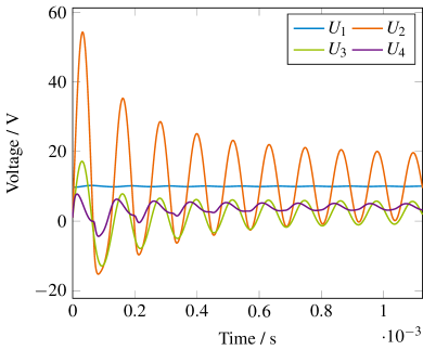
Figure 3: Left: Transient behavior of the Colpitts oscillator until the steady state. Right: Convergence of the PP-PC approach with a linearized coarse grid problem for the case when the period $T$ is given Kulchytska-Ruchka_2019ag and of PP-PC-UP when $T$ is unknown (3).

The transient behavior of the oscillator on $[0,1.125]$ $\text{\,}\mathrm{ms}$ is shown in Fig. 3 on the left. The time step $\delta T=$0.1125\text{\,}\mathrm{\SIUnitSymbolMicro s}$$ and the initial value at $t=0$ is $\mathbf{u}_{0}=[9.75,1,1,1]^{\top}$ are chosen.

To find the periodic steady-state solution and the corresponding period $T$ we apply the iteration (14). Linearization of the nonlinear periodic system on the coarse level is performed using a surrogate linear model, i.e., $\bar{\mathcal{G}}$ solves the problem (13) with $\bar{\mathbf{f}}(\mathbf{U})=\mathbf{A}\mathbf{U}+\mathbf{c}$ given by

$$\mathbf{A} =\begin{bmatrix}-R_{2}/L&R2/L&&\\ -1/R_{2}&-x_{\mathrm{C}}/\bar{U}_{\mathrm{T}}&I_{\mathrm{S}}/\bar{U}_{\mathrm{T}}&(x_{\mathrm{C}}-I_{\mathrm{S}})/\bar{U}_{\mathrm{T}}\\ 0&I_{\mathrm{S}}/\bar{U}_{\mathrm{T}}&-1/R_{4}-x_{\mathrm{E}}/\bar{U}_{\mathrm{T}}&(x_{\mathrm{E}}-I_{\mathrm{S}})/\bar{U}_{\mathrm{T}}\\ 0&y_{\mathrm{C}}/\bar{U}_{\mathrm{T}}&y_{\mathrm{E}}/\bar{U}_{\mathrm{T}}&-1/R_{3}-1/R_{1}-y_{\mathrm{E}}/\bar{U}_{\mathrm{T}}-y_{\mathrm{C}}/\bar{U}_{\mathrm{T}}\end{bmatrix},$$ (17)

$$\mathbf{c} =\left[0,U_{\mathrm{op}}/R_{2},0,U_{\mathrm{op}}/R_{1}\right]^{\top},$$ (18)

with $\bar{U}_{\mathrm{T}}=$0.2585\text{\,}\mathrm{V}$.$ The unit interval $[0,1]$ is split into $N=10$ windows. The coarse time step $\Delta\tau=0.1$ and the fine step $\delta\tau=10^{-4}$ were chosen within the time integration. The calculated period with the fixed point iteration (3) is $T=$0.1125\text{\,}\mathrm{ms}$.$ The right-hand part of the Fig. 3 shows convergence of the PP-PC iteration with the linearization from Kulchytska-Ruchka_2019ag for a given period $T$ as well as for an unknown period (PP-PC-UP). Both results are obtained up to the relative tolerance of $10^{-3}.$ One can see that in case when $T$ is known the method required less iterations, as one would expect. When comparing the computational cost of the computations in terms of the number of linear systems solves, PP-PC and PP-PC-UP delivered the periodic solution effectively $4$ and $3$ times faster than the sequential time stepping, respectively.

5 Conclusions

An iterative parallel-in-time method for solving time-periodic problems where the period is not initially given is proposed in this paper. It complements the system of equations originating from the Parareal-like algorithm with an additional variable $T$ and gives an underdetermined system of nonlinear equations. A linearization using the fixed point iteration is applied on the coarse grid. The algorithm is verified through its application to a Colpitts oscillator model.

- [1] A. Bermúdez, D. Gómez, M. Piñeiro, and P. Salgado. A novel numerical method for accelerating the computation of the steady-state in induction machines. Comput. Math. Appl., 79(2):274–292, 2019.
- [2] O. Bíró and K. Preis. An efficient time domain method for nonlinear periodic eddy current problems. IEEE Trans. Magn., 42(4):695–698, 2006.
- [3] P. Deuflhard. Computation of periodic solutions of nonlinear ODEs. BIT, (24):456–466, 1984.
- [4] P. Deuflhard. Newton methods for nonlinear problems: affine invariance and adaptive algorithms. Springer, Berlin, 2004.
- [5] R. D. Falgout, S. Friedhoff, T. V. Kolev, S. P. MacLachlan, and J. B. Schroder. Parallel time integration with multigrid. SIAM J. Sci. Comput., 36(6):C635–C661, 2014.
- [6] M. J. Gander, Y.-L. Jiang, B. Song, and H. Zhang. Analysis of two parareal algorithms for time-periodic problems. SIAM J. Sci. Comput., 35(5):A2393–A2415, 2013.
- [7] M. J. Gander and S. Vandewalle. Analysis of the parareal time-parallel time-integration method. SIAM J. Sci. Comput., 29(2):556–578, 2007.
- [8] T. Hara, T. Naito, and J. Umoto. Time-periodic finite element method for nonlinear diffusion equations. IEEE Transactions on Magnetics, 21(6):2261–2264, 1985.
- [9] W. Kampowsky, P. Rentrop, and W. Schmidt. Classification and numerical simulation of electric circuits. Surv. Math. Ind., 2(1):23–65, 1992.
- [10] I. Kulchytska-Ruchka and S. Schöps. Efficient parallel-in-time solution of time-periodic problems using a multi-harmonic coarse grid correction, 2019. ArXiv: 1908.05245.
- [11] J.-L. Lions, Y. Maday, and G. Turinici. A parareal in time discretization of PDEs. Comptes Rendus de l’Académie des Sciences – Series I – Mathematics, 332(7):661–668, 2001.
- [12] R. Mirzavand Boroujeni, E. J. W. ter Maten, T. G. J. Beelen, W. H. A. Schilders, and A. Abdipour. Robust periodic steady state analysis of autonomous oscillators based on generalized eigenvalues. In: B. Michielsen, J.-R. Poirier (eds.), Scientific Computing in Electrical Engineering SCEE 2010, Mathematics in Industry, vol. 16, pp. 293–302, 2012.
- [13] D. D. Morrison, J. D. Riley, and J. F. Zancanaro. Multiple shooting method for two-point boundary value problems. Comm. ACM, 5(12):613–614, 1962.
- [14] R. Pulch. Multi time scale differential equations for simulating frequency modulated signals. APNUM, 53(2–4):421–436, 2005.
- [15] Y. Takahashi, T. Tokumasu, A. Kameari, H. Kaimori, M. Fujita, T. Iwashita, and S. Wakao. Convergence acceleration of time-periodic electromagnetic field analysis by singularity decomposition-explicit error correction method. IEEE Trans. Magn., 46(8):2947–2950, 2010.