Pion and Kaon parton distributions in the QCD instanton vacuum

Abstract

We discuss a general diagrammatic description of n-point functions in the QCD instanton vacuum that resums planar diagrams, enforces gauge invariance and spontaneously broken chiral symmetry. We use these diagrammatic rules to derive the pion and kaon quasi-parton amplitude and distribution functions at leading order in the instanton packing fraction for large but finite momentum. The instanton and anti-instanton zero modes and non-zero modes are found to contribute to the quasi-distributions, but the latter are shown to drop out in the large momentum limit. The pertinent pion and kaon parton distribution amplitudes and functions are made explicit at the low renormalization scale fixed by the inverse instanton size. Assuming that factorization holds, the pion parton distributions are evolved to higher renormalization scales with one-loop DGLAP and compared to existing data.

I Introduction

Light cone distribution amplitudes are central to the description of hard exclusive processes with large momentum transfer. They account for the non-perturbative quark and gluon content of a hadron in the infinite momentum frame. Using factorization, hard cross sections can be split into soft partonic distributions convoluted with perturbativly calculable processes. The soft partonic distributions are inherently non-perturbative. They can be extracted through moments using experiments FF , or more recently lattice simulations JI ; JI1 .

Several QCD lattice simulations have suggested that the bulk characteristics and correlations of the light hadronic operators are mostly unaffected by lattice cooling CHU , strongly suggesting that semi-classical gauge and fermionic fields maybe dominant in the ground state. At weak coupling, instantons and anti-instantons are exact classical gauge tunneling configurations with large actions and finite topological charge which support exact quark zero modes with specific chirality.

Extensive calculations both analytically and numerically DP ; IQCD ; MF , describing the QCD ground state as an ensemble of instantons and anti-instantons with hopping quark zero modes where found to reproduce most of the cooled lattice simulations. In the quenched approximation, these calculations can be organized by observing that the ensemble is characterized by a small packing fraction in the large $N_{c}$ limit which is dominated by planar graphs.

The twist-2 pion distribution amplitude and function have been discussed in the context of the QCD sum rules M1 , bottom-up holographic models BROD , bound state re-summations M3 , basis light front quantization using an effective Nambu-Jona-Lasinio (NJL) interaction BASIS , covariant NJL models with effective interactions BRO , and the instanton model using non-local effective interactions and modified dipole-like or gaussian quark masses time-like LAW1 ; LAW2 .

The instanton model for the QCD vacuum is inherently space-like. It is amenable to QCD through semi-classics and allows for an organizational principle that enforces chiral ang gauge Ward identities. It is well suited for the description of the bulk of the QCD vacuum with its its flavor singlet axial and scale anomalies, and its mesonic and baryonic excitations through pertinent Euclidean correlators DP ; IQCD ; MF . However, its inherent Euclidean character makes it difficult to characterize the non-perturbative time-like structure of its partonic constituents as probed by deep inelastic scattering.

The recent suggestion put forth by Ji JI and its matching protocol JI2 , to extract the light cone distribution functions from equal-time quasi-distributions in Euclidean space, has been carried on the lattice with some reasonable success LATTICE . This formulation makes the instanton calculus amenable to a first principle semi-classical analysis of the quasi-distributions, and therefore the light cone distributions by matching. Since the distribution functions obey sum rules, the enforcement of the Ward identities is important. This can be sought through a diagrammatic expansion and power counting around the planar approximation, both of which preserve chiral and gauge invariance. We note that recently, the quasi-pion distribution functions were analyzed using some of the models described above RAD ; QUASI .

The purpose of this paper is to revisit the n-point functions in the random instanton vacuum (RIV) in the planar approximation as in POB . The latter resums a large class of instanton contributions in the form of non-perturbative integral equations with full chiral and gauge symmetry. While these equations are in general involved and require a numerical analysis, we will analyze them relying on the diluteness of the instantons and anti-instantons in the QCD vacuum, where the packing fraction is small with $\kappa\approx 10^{-3}$. All calculations will be carried at leading order (LO) and/or next to leading order (NLO) in $\alpha\approx\sqrt{\kappa}$.

This expansion provides an organizational principle and addresses some of the shortcomings in DP ; MF by enforcing the axial and vector Ward identities in the planar approximation. It turns out that the zero modes and non-zero modes are equally important in this enforcement, as initially noted for the 2-point vector correlator in GROSS . Also, the virtual character of the induced effective quark constituents generated by the planar resummation makes their time-like manifestation in the pion distribution amplitude and function very subtle.

This paper consists of several new results in the QCD random instanton vacuum (RIV): 1/ a generalization of the planar resummation to the n-point functions; 2/ an explicit derivation of the 2- and 3-point functions at NLO; 3/ a derivation of the quark effective mass at NLO; 4/ a planar re-summation of the pion quasi-parton amplitude and distribution functions at LO; 5/ explicit expressions for the pion and kaon PDA, PDF and TMD at LO; 6/ an explicit proof of the axial Ward identity for the axial-axial correlation function at NLO; 7/ an explicit evolution of the pion PDA, PDF and TMD and comparison with currently available data.

The organization of the paper is as follows: in section II we briefly review the general aspects of the random instanton vacuum, and detail the planar approximation for the derivation of the quark propagator. We derive the induced effective quark mass and in general spin-valued self-energy at NLO. In section III we show how the 2-point meson correlators are re-summed, and use the result to derive the pion pseudo-scalar vertex at NLO. The pion decay constant is worked out in the leading logarithm approximation. In section IV we derive the pion QPDA in LO in the leading logarith approximation and beyond. In section V we show how the planar re-summation applies to the 3-point functions and use it to construct the pion QPDF, PDF and TMD also at LO. All the results are QCD evolved and compared to available data. Our conclusions are in section VI. A number of details can be found in several Appendices, including the LO result for the GPDF.

II Quark propagator

Key to the analysis of the spontaneous breaking of chiral symmetry in the random instanton vacuum is the appearance of a momentum dependent constituent mass dynamically. To illustrate this, consider the quark propagator in the chiral limit and the quenched approximation of QCD

$$\left<\psi(x)\psi^{\dagger}(y)\right>=\bigg{<}\left<x|(-i\not{\partial}-\not{A}-im)^{-1}|y\right>\bigg{>}_{A}$$ (1)

where the averaging is over the gauge configurations $A$. In the instanton vacuum, the gauge configurations are restricted to the semi-classical set of instantons and anti-instantons which are sampled either random (random instanton model) or through their semi-classical interactions (interacting instanton model). Throughout, we will refer to the instanton liquid model as the random instanton model. With this in mind and to enforce topological neutrality of the vacuum, the semi-classical configurations are chosen to be $\frac{N}{2}$ instantons and $\frac{N}{2}$ anti-instantons non-interacting and randomly distributed in a 4-volume $V_{4}$, with

$$A=\sum_{I=1}^{\frac{N}{2}}A_{I}+\sum_{\bar{I}=1}^{\frac{N}{2}}A_{\bar{I}}$$ (2)

Each of the instanton and anti-instanton $A_{I,\bar{I}}$ in (2) is an SU(2) valued matrix embedded in SU($N_{c}$) with arbitrary orientation $U_{I,\bar{I}}$ in color space and position $z_{I,\bar{I}}$ in 4-space. For simplicity, all instantons are chosen to carry the same size $\rho\approx 1/3$ fm with a density fixed at $n=N/V_{4}\approx 2\,{\rm fm}^{-4}$. In Fig. 1 we show the instanton size distribution versus their size $\rho$ in fm from the instanton liquid model in comparison to SU(2) lattice simulations IQCD MICHAEL .

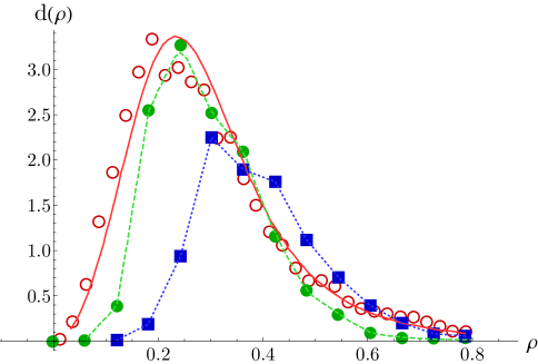
Figure 1: Instanton size distribution in pure SU(2) gauge theory calculated on the lattice MICHAEL and in the interacting instanton liquid model (IILM) IQCD . The unit scale is fm. Closed points correspond to lattice data with decreasing lattice spacing. Open points are from an IILM calculation. The solid line is a parameterization of the IILM result as discussed in IQCD . The dotted and dashed lines simply aid the eye. In both pure SU(2) and pure SU(3), an average value $\rho\approx 1/3\,\textrm{fm}$ is found.

In the semiclassical background (2) the quark propagator can be organized as an expansion in multiple re-scatterings with increasing number of instantons and anti-instantons

$$S-S_{0}=\bigg{<}\sum_{I}S_{I}-S_{0}+\sum_{I\neq J}(S_{I}-S_{0})S_{0}^{-1}(S_{J}-S_{0})+\sum_{I\neq J,J\neq K}(S_{I}-S_{0})S_{0}^{-1}(S_{J}-S_{0})S_{0}^{-1}(S_{K}-S_{0})+..\bigg{>}$$ (3)

Here $S_{0}=1/(-i\not{\partial}-im)$ is the free quark propagator, $S_{I}=1/(-i\not{\partial}-\not{A}_{I}-im)$ is the quark propagator in a single instanton or anti-instanton background and the sum is over all instantons and anti-instantons. The averaging means independent integrations over the instanton and anti-instanton positions and color orientations.

II.1 Planar re-summation

Large $N_{c}$ QCD is essentially a quenched approximation dominated by planar graphs. The same applies to its semi-classical approximation in terms of a random instanton vacuum, if we note that $n\sim N_{c}$ and that the averaging over the SU($N_{c}$) color orientations bring extra factors of $1/N_{c}$. The planar contributions to the quark propagator are re-summed through the formal equation POB

$$S-S_{0}=\frac{N}{2V_{4}}\int_{I+\bar{I}}dz_{I}dU_{I}\left(\frac{1}{1-S_{\not{I}}\Delta}\right)S_{\not{I}}S_{0}^{-1}S=\frac{N}{2V_{4}}\int_{I+\bar{I}}dz_{I}dU_{I}\,S_{0}\left(\frac{1}{S_{0}S_{\not{I}}^{-1}S_{0}-S_{0}\Delta S_{0}}\right)S$$ (4)

with the single instanton (anti-instanton) propagator $S_{I}=S_{0}+S_{\not{I}}$ , and the amputated and re-summed propagator

$$S_{0}^{-1}SS_{0}^{-1}=\Delta+S_{0}^{-1}$$ (5)

The integrations in (4) is over the instanton moduli for fixed instanton size. The integration over the rigid gauge color $U_{I}$ projects onto the color singlet channel, while the integration over the global 4-position $z_{I}$ restores translational invariance. (4) is readily recast in the form

$$S^{-1}-S_{0}^{-1}=\frac{N}{2V_{4}}\int_{I+\bar{I}}dz_{I}dU_{I}\left(\frac{1}{S-S_{0}(S_{0}^{-1}+S_{\not{I}}^{-1})S_{0}}\right)$$ (6)

Inserting the identity

$$S_{\not{I}}^{-1}=\frac{1}{S_{I}-S_{0}}=S_{0}^{-1}(-A_{I})^{-1}S_{I}^{-1}$$ (7)

in (6) yields a formal integral equation for the self-energy POB

$$S^{-1}-S_{0}^{-1}=\frac{N}{2V_{4}}\int_{I+\bar{I}}dz_{I}dU_{I}\frac{1}{S-\not{A_{I}}^{-1}}\equiv\frac{N}{2V_{4}}\int_{I+\bar{I}}dz_{I}dU_{I}\,\Sigma_{I}$$ (8)

which sums over a single instanton plus anti-instanton. The SU($N_{c}$) averaging in (8) over $U_{I}$ projects onto the color singlet channel, and the z-integral restores translational invariance. Throughout and for simplicity, only the massless case will be considered with $m=0$ unless specified otherwise.

For $S^{-1}-S_{0}^{-1}=-i\sigma$, (8) takes the formal gap-like form

$$i\sigma=\frac{N}{2N_{c}V_{4}}\int_{I+\bar{I}}dz_{I}\,{\rm Tr}_{C}\bigg{(}\not{A_{I}}\frac{1}{i\not{\partial}+\not{A_{I}}+i\sigma}(i\not{\partial}+i\sigma)\bigg{)}$$ (9)

with ${\rm Tr}_{C}$ referring to the color trace (in some places below it will also mean spin as well). The small parameter $\kappa$ or packing fraction,

$$\kappa=\frac{N\rho^{4}}{2V_{4}N_{c}}\equiv\alpha^{2}\rho^{4}\approx 3.186\,\times 10^{-3}$$ (10)

is of order $N_{c}^{0}$ provided that the instanton density is made to scale as $N/V_{4}\sim N_{c}$.

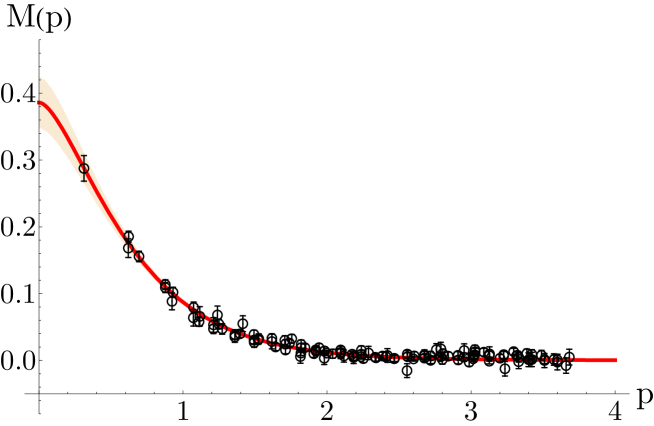
Figure 2: Momentum dependence of the instanton induced effective quark mass in singular gauge (13) at LO (solid-curves), compared to the effective quark mass measured on the lattice in Coulomb gauge BOWMAN (open-circles). The unit scale is GeV. We obtain a fitted parameter intervals $M(0)=383\pm 39$ MeV and $\rho=0.313\pm 0.016$ fm.

II.2 Effective mass at LO

The effective mass operator (8) can be sought iteratively $\sigma=\alpha\sigma_{0}+\alpha^{2}\sigma_{1}+...$, with a starting correction of order $\alpha$ and not $\alpha^{2}$ POB . In leading order (LO),

$$\Delta_{I}(x,y)\equiv\left<x\right|\frac{1}{i\not{\partial}+\not{A_{I}}+i\alpha\sigma_{0}}\left|y\right>=\frac{\psi_{0I}(x)\psi_{0I}^{\dagger}(y)}{i\alpha\sigma_{00}}+{\cal O}(\alpha)$$ (11)

with $\sigma_{00}=\left<0|\sigma_{0}|0\right>=\sqrt{2}||q\varphi^{\prime 2}||\sim\rho$, the expectation value of $\sigma_{0}$ in the zero mode state $\psi_{0I}$. Its form is given in Appendix A both in regular and singular gauge. The norm notation is subsumed. Inserting (11) into (9) yields the effective mass at LO

$$M(p)\approx\alpha\sigma_{0}(p)=\frac{\alpha}{\sigma_{00}}{\rm Tr}_{C}\left(\not{p}\left(\psi_{0I}(p)\psi_{0I}^{\dagger}(p)+\psi_{0\bar{I}}(p)\psi_{0\bar{I}}^{\dagger}(p)\right)\not{p}\right)\equiv\frac{\alpha}{\sigma_{00}}{\rm Tr}_{C}\left({\not{p}\left(P_{I}(p)+P_{\bar{I}}(p)\right)\not{p}}\right)=\frac{\alpha}{\sqrt{2}}\frac{|p\varphi^{\prime}(p)|^{2}}{||q\varphi^{\prime 2}||}$$

with $P_{I}$ the zero mode projector. After color tracing, the effective mass operator is diagonal in spin. The last relation holds for both the regular and singular gauge, but with different zero mode profiles. In singular gauge from Appendix A we have

$$\frac{M(p)}{M(0)}=\bigg{(}\left|z\left(I_{0}K_{0}-I_{1}K_{1}\right)^{\prime}\right|^{2}\bigg{)}_{z=\frac{1}{2}\rho p}$$ (13)

The effective mass is not analytic in the packing fraction since $\alpha\sim\sqrt{\kappa}$. In Fig. 2 we show (II.2) for $M(0)=383$ MeV and $\rho=0.313$ fm in solid-red curve in comparison to the lattice generated effective quark mass in Coulomb gauge BOWMAN . The spread corresponds to a $99\%$ confidence interval generated by a standard weighted least squares regression on the data in Fig. 2, giving parameter ranges $M(0)=383\pm 39$ MeV and $\rho=0.313\pm 0.016$ fm. At large momenta, $M(p)\approx 1/p^{6}$ falls faster than $\alpha^{D}_{s}(p^{2})/p^{2}$ with $D=39/27$ derived using short distance QCD arguments POLITZER , but in good agreement with the lattice results.

II.3 Effective mass at NLO

At next to leading order (NLO) the effective mass is obtained by further expanding (11) and keeping the contributions to order $\alpha$. For that, we can organize (11) formally so that

$$\Delta_{I}= \frac{1}{i\not{\partial}+\not{A_{I}}+i\alpha\sigma_{00}}+\frac{1}{i\not{\partial}+\not{A_{I}}+i\alpha\sigma_{00}}(-i\alpha(\sigma_{0}-\sigma_{00}))\,\Delta_{I}$$

$$= \bigg{(}\frac{P_{I}}{i\alpha\sigma_{00}}+G_{I}\bigg{)}+\bigg{(}\frac{P_{I}}{i\alpha\sigma_{00}}+G_{I}\bigg{)}(-i\alpha(\sigma_{0}-\sigma_{00}))\,\Delta_{I}$$ (14)

with $P_{I}$ the projector on the quark zero mode, and $G_{I}$ the quark non-zero mode propagator in the instanton background. Using the virtual quark eigenstates $(i\not{\partial}+\not{A_{I}})\psi_{kI}=E_{k}\psi_{kI}$ and the mode expansion for $G_{I}=\sum_{k\neq 0}\psi_{kI}\psi^{\dagger}_{kI}/E_{k}$ we can explicitly solve for $\Delta_{I}$ at NLO

$$\Delta_{I}= \frac{P_{I}}{i\alpha\sigma_{00}}+\sum_{k\neq 0}\frac{\psi_{kI}\psi_{kI}^{\dagger}}{E_{k}}+P_{I}\sum_{k\neq 0}\frac{\sigma_{0k}\sigma_{k0}}{E_{k}\sigma_{00}}-\sum_{k\neq 0}\frac{\psi_{kI}\psi_{0I}^{\dagger}\sigma_{k0}}{E_{k}\sigma_{00}}-\sum_{k\neq 0}\frac{\psi_{0I}\psi_{kI}^{\dagger}\sigma_{0k}}{E_{k}\sigma_{00}}+{\cal O}(\alpha)$$ (15)

The matrix elements $\sigma_{kl}=\left<k|\sigma|l\right>$ involve $\sigma$ only in leading order or $\sigma_{0}$. From (9) the self-energy at NLO is spin-valued and reads

$$\Sigma_{I} = \not{A_{I}}\frac{-1}{i\not{\partial}+\not{A_{I}}+i\sigma}(i\not{\partial}+i\sigma)$$ (16)

$$\approx i\not{\partial}\frac{P^{I}}{i\alpha\sigma_{00}}i\not{\partial}+i\not{\partial}(1-P^{I}\hat{\sigma})G^{I}(1-\hat{\sigma}P^{I})i\not{\partial}-i\not{\partial}+i\not{\partial}P^{I}\hat{\sigma}+\hat{\sigma}P^{I}i\not{\partial}-\frac{\beta_{00}}{i\sigma_{00}^{2}}i\not{\partial}P^{I}i\not{\partial}\approx\frac{\Sigma_{I0}}{\alpha}+\Sigma_{I1}$$

with $\hat{\sigma}={\sigma_{0}}/{\sigma_{00}}$. The last contribution was added to account for the planar re-summation to the self-energy through the gap-equation

$$-i\beta_{00}(p)=\int d^{4}x\,d^{4}y\,e^{ip\cdot(x-y)}\,{\rm Tr}_{C}\Sigma_{I1}(x,y)={\rm Tr}_{C}\Sigma_{I1}(p,p)$$ (17)

The anti-instanton contribution follows through the substitution $I\rightarrow\bar{I}$. The effective mass at NLO follows by substituting (16) in (9) which is now a true gap-equation because of the contribution (17). The first contribution is in agreement with (II.2). The non-zero mode contribution $G_{I}$ in (16) is important for the enforcement of symmetries at NLO. Its explicit form in singular gauge is given in Appendix A.

III Mesonic vertices in the planar approximation

In this section we formulate the planar resummation for the 2-point functions. We will focus on flavor singlet correlators with a single flavor and ignore vacuum loops, with the assumption that we are evaluating non-singlet flavor correlators where the loop corrections are suppressed by $1/N_{c}$. We will analyze in details the resummation for the 2-point pseudoscalar source at LO and NLO.

III.1 Meson correlators

The T-matrix in the planar approximation for re-scattering of two quarks in the $2\rightarrow 2$ channel, can be constructed using formally the 2PI kernel

$$K=\frac{N}{2V}\int_{I+\bar{I}}dz_{I}dU_{I}\,\bigg{(}\Sigma_{I}\otimes\Sigma_{I}\bigg{)}$$ (18)

with the color-spin-space valued self-energy $\Sigma_{I}$ given in (8). We can now use the 2PI kernel to construct any 2-point correlation function in the QCD instanton vacuum. For that, consider the general local and colorless source $J_{\Gamma}=\psi^{\dagger}\Gamma\psi$, say for a meson of spin-flavor $\Gamma$, and define the amputated spin-flavored valued operator

$$O_{\Gamma\,ab}(P,k)=$$

$$S^{-1}(k)\left<\psi_{a}(k)\psi_{b}^{\dagger}(P-k)J_{\Gamma}(P)\right>S^{-1}(k-P)$$

where the averaging is carried over the instanton-anti-instanton vacuum gauge configurations. (III.1) refers to a quark of color-spin-a and momentum $k$ combining with a quark of color-spin-b and momentum $P-k$ to give a colorless meson of spin-$\Gamma$ and momentum $P$.

The resummed instanton contributions to (III.1) in the planar approximation can be obtained by tracing (III.1) with the 2PI kernel (18) with the result

$$O_{\Gamma}(P,k)=\Gamma+\alpha^{2}\rho^{4}\sum_{I+\bar{I}}\int\frac{d^{4}p}{(2\pi)^{4}}\,{\rm Tr}_{C}\bigg{(}\Sigma_{I}(k,p)S(p)O_{\Gamma}(P,p)S(p-P)\Sigma_{I}(p-P,k-P)\bigg{)}$$ (20)

The net effect of averaging over the instanton-anti-instanton ensemble is the projection onto the color singlet channel and momentum conservation. (200 is the analogue of the Bethe-Salpeter equation for the vertex functions. Using (20) the re-summed 2-point function for an arbitrary meson correlator in the planar approximations is

$${\cal C}_{\Gamma_{1}\Gamma_{2}}(P)\equiv\left<O_{\Gamma_{1}}(-P)O_{\Gamma_{2}}(P)\right>=-\int\frac{d^{4}k}{(2\pi)^{4}}\,{\rm Tr}_{C}\bigg{(}\Gamma_{1}S(k)O_{\Gamma_{2}}(P,k)S(k-P)\bigg{)}$$ (21)

III.2 Pseudo-scalar pion vertex at LO

The leading-order $\alpha$ contribution to the pion pseudoscalar correlator can be obtained by setting $\Gamma=\gamma_{5}$, $\Sigma_{I}\sim\Sigma_{0}/\alpha$ and $S\sim 1/(\not{k}-i\alpha\sigma_{0}(0))$ in (20-21). As we will show below, many of our expressions will in fact be (logarithmically) divergent in $\alpha$. We will encounter integrals of the form ($n\geq 2$)

$$\int\frac{d^{4}k}{(2\pi)^{4}}\frac{F(k)}{\left(k^{2}+\alpha^{2}\sigma_{0}^{2}(0)\right)^{n}}$$ (22)

where $F(k)$ is a smooth function that approaches a constant value as $k^{2}\rightarrow 0$ and rapidly drops off as $k^{2}\gg\rho^{-2}$. To extract the leading contribution in $\alpha$ from the integral of this kind, we may shift $k^{2}\rightarrow k^{2}-\alpha^{2}\sigma_{0}^{2}(0)$, and subsequently drop corrections to $F(k^{2}-\alpha^{2}\sigma_{0}^{2}(0))\approx F(k^{2})$ which only contribute subleading divergent corrections (e.g. $\alpha\log(\alpha)$, $\alpha^{2}\log(\alpha)$, etc.). As will prove useful later, it is totally equivalent to instead only shift $k_{\perp}^{2}\rightarrow k_{\perp}^{2}-\alpha^{2}\sigma_{0}^{2}(0)$, which then leads to a shift in the lower bound of integration of only $k_{\perp}^{2}$.

$$k_{\perp}^{2}>\alpha^{2}\sigma_{0}^{2}(0)=M^{2}(0)$$ (23)

With this in mind, a formal solution follows for the vertex operator $O_{5}(P,k)\approx\gamma^{5}F_{5}(P,k)$, with the vertex function $F_{5}(P,k)$ diagonal in spin space. In singular gauge, the latter formally satisfies the integral equation

$$\gamma^{5}F_{5}(P,k)=\gamma^{5}+\frac{\varphi^{\prime}(k)\varphi^{\prime}(k-P)|k||k-P|}{\sigma_{00}^{2}}\,\int\frac{d^{4}p}{(2\pi)^{4}}F_{5}(P,p)\left(-\psi_{I}^{\dagger}(p)\psi_{I}(p-P)\frac{1-\gamma_{5}}{2}+\psi_{\bar{I}}^{\dagger}(p)\psi_{\bar{I}}(p-P)\frac{1+\gamma_{5}}{2}\right)$$

This is a Fredholm integral equation of the second-kind, and can be solved with a Liouville-Neumann series, which is found to be geometric. The solution then follows by summation with the result

$$F_{5}(P,k)=1+\lambda(P)\frac{\varphi^{\prime}(k)\varphi^{\prime}(k-P)|k||k-P|}{\sigma_{00}^{2}}$$ (25)

with $\lambda(P)$ satisfying

$$\lambda(P)\bigg{(}1-\frac{2}{\sigma_{00}^{2}}\,{\int\frac{d^{4}k}{(2\pi)^{4}}\varphi^{\prime 2}(k)\varphi^{\prime 2}(k-P)(k^{2}-k\cdot P)}\bigg{)}=1$$

For small momentum we have $\lambda(P)\approx(\sqrt{N_{c}}/f_{\pi})/P^{2}$, corresponding to the pion pole in the chiral limit. We note that the LO contribution (25) amounts to the effective coupling at the pion pole

$$\bigg{(}iO_{5}(P,k)\bigg{)}_{P^{2}\approx 0}\approx\frac{\sqrt{N_{c}}}{f_{\pi}}\sqrt{M(k)}\left(\frac{i\gamma_{5}}{P^{2}}\right)\sqrt{M(k-P)}$$

with the running mass of order $\alpha$ given in (II.2). This LO result is in agreement with the effective vertex following from the partially resummed planar diagrams in DP ; IQCD ; MF . (25) gives the full pion pseudoscalar vertex on- and off-mass-shell in the massless limit. The massive case will be discussed below.

III.3 Pion decay constant $f_{\pi}$ at LO

The explicit values of $g_{\pi},f_{\pi}$ follow from the pseudo-scalar two-point correlation function (21) with the vertex function (25), which is of order $\alpha^{0}$ to LO. More specifically, the pion pole contribution reads

$${\cal C}_{\gamma_{5};\gamma_{5}}(P)\approx-\int\frac{d^{4}k}{(2\pi)^{4}}{\rm Tr}\left(\gamma_{5}F_{5}(P,k)\frac{1}{\not{k}}\gamma_{5}\frac{1}{\not{k}-\not{P}}\right)\approx\frac{g_{\pi}^{2}}{P^{2}}$$

$g_{\pi}$ defines the pseudoscalar pion-quark-quark coupling and in LO is given by

$$g_{\pi}^{2}=-N_{c}\left(\int\frac{d^{4}k}{(2\pi)^{4}}\left(3\,\varphi^{\prime 4}+7(k\rho)\,\varphi^{\prime 3}\varphi^{\prime\prime}+{(k\rho)^{2}}\left(\varphi^{\prime 3}\varphi^{\prime\prime\prime}+\varphi^{\prime 2}\varphi^{\prime\prime 2}\right)\right)\right)^{-1}$$ (29)

The pion decay constant $f_{\pi}$ is related to $g_{\pi}$ in (29) by chiral reduction with

$$f_{\pi}g_{\pi}=-2i\left<\psi^{\dagger}\psi\right>\approx 2N_{c}\frac{M(0)}{(2\pi\rho)^{2}}$$ (30)

in leading order in the current quark mass. The last identity is the LO contribution to the chiral condensate, and is the expected Goldberger-Treiman relation for the effective quark coupling. (30) is infrared finite and of order $\alpha$. Both $f_{\pi},g_{\pi}$ are infrared sensitive with

$$g_{\pi}^{2}\approx N_{c}\bigg{(}\int\frac{d^{4}k}{(2\pi)^{4}}\frac{(2\pi\rho)^{4}}{k^{4}}\bigg{)}^{-1}$$ (31)

and similarly for $f_{\pi}$

$$f_{\pi}^{2}\approx 4N_{c}\int\frac{d^{4}k}{(2\pi)^{4}}\,\frac{M^{2}(0)}{k^{4}}$$ (32)

Note that $g_{\pi}$ in (29) and therefore $f_{\pi}$ in (30) are UV finite with an approximate range of $1/\rho$. The infrared sensitivity follows from the shift which led to (23). This shift will be understood throughout.

To logarithmic accuracy $g_{\pi}^{2}\sim N_{c}/{\rm ln}(1/\alpha)$ and $f_{\pi}^{2}\sim N_{c}\alpha^{2}{\rm ln}(1/\alpha)$ with

$$f_{\pi}^{2}\approx\frac{N_{c}M^{2}(0)}{2\pi^{2}}\,{\rm ln}\bigg{(}\frac{C}{\rho M(0)}\bigg{)}$$ (33)

modulo a constant $C$ of order 1. $f_{\pi}^{2}$ captures the chiral conductivity in the QCD vacuum RANDOM . Using the values of $M(0)\rho$ displayed in Fig. 2 we have $C=0.849$ for $f_{\pi}=86\,\textrm{MeV}$ in the chiral limit, $C=0.897$ for $f_{\pi}=93\,\textrm{MeV}$ for massive pions, and $C=1.04453$ for $f_{K}=110\,\textrm{MeV}$ for massive kaons (see below).

III.4 Pseudo-scalar pion vertex at NLO

The pseudo-scalar pion vertex can be sought at NLO using

$$O_{5}(P,k)=\gamma^{5}\bigg{(}1+F_{5}(P,k)\bigg{)}+\alpha\overline{F}_{5}(P,k)+{\cal O}(\alpha^{2})$$ (34)

in (20) and the explicit form of the spin-valued self-energy (16) at NLO. The result is

$$\overline{F}_{5}(P,k)=K_{\pi}\overline{F}_{5}(P,k)$$

$$+\rho^{4}\sum_{I+\bar{I}}\int\frac{d^{4}p}{(2\pi)^{4}}{\rm Tr}_{C}\bigg{(}\Sigma_{I1}(k,p)S_{0}(p)\gamma^{5}{F}_{5}(P,p)S_{0}(p_{-})\Sigma_{I0}(p_{-},k_{-})+\Sigma_{I0}(k,p)S_{0}(p)\gamma^{5}{F}_{5}(P,p)S_{0}(p_{-})\Sigma_{I1}(p_{-},k_{-})\bigg{)}$$

with $k_{-},p_{-}=k-P,p-P$. The reduced kernel $K_{\pi}$ involves only the zero modes and satisfies

$$K_{\pi}O=\rho^{4}\sum_{I,\bar{I}}\int\frac{d^{4}p}{(2\pi)^{4}}{\rm Tr}_{C}\bigg{(}\Sigma_{I0}(k,p)S_{0}(p)OS_{0}(p_{-})\Sigma_{I0}(p_{-},k_{-})\bigg{)}$$

(III.4) defines formally an integral-type equation for the spin-valued operator $\overline{F}_{5}(P,k)$. The homogeneous part does not iterate due to a mismatch in chirality. In the inhomogeneous contribution, we note that most of the contributions in $\Sigma_{I1}$ as given in (16) do not contribute due to a mismatch in chirality except for $\delta G_{I}=G_{I}-S_{0}$, thus the result

$$\overline{F}_{5}(P,k)= \sum_{I+\bar{I}}\int\frac{d^{4}p}{(2\pi)^{4}}{\rm Tr}_{C}\left(\not{k}\delta G_{I}(k,p)\gamma^{5}F_{5}(P,p)\psi_{0I}(p_{-})\frac{1}{i\sigma_{00}}\psi_{0I}^{\dagger}(k_{-})\not{k}_{-}\right)$$

$$+ \sum_{I+\bar{I}}\int\frac{d^{4}p}{(2\pi)^{4}}{\rm Tr}_{C}\left(\not{k}\psi_{0I}(k)\frac{1}{i\sigma_{00}}\psi^{\dagger}_{0I}(p)\gamma^{5}F_{5}(P,p)\delta G_{I}(p_{-},k_{-})\not{k}_{-}\right)$$ (37)

It may be checked that the non-vanishing spin-valued structures of (III.4) are of the type $\gamma_{5}\not{P}$ and $\gamma_{5}\not{k}$ times invariant scalars. For estimates, we may use $\delta G_{I}$ in the Born approximation (singular gauge)

$$\delta G_{I}(k,p)\rightarrow\frac{1}{S_{0}^{-1}+i\not{A}}_{I}-S_{0}\approx-iS_{0}\not{A}_{I}S_{0}\approx iS_{0}\bigg{(}\frac{\gamma^{M}{\bar{\sigma}}^{MN}x^{N}\rho^{2}}{(x^{2}+\rho^{2})x^{2}}\bigg{)}S_{0}\rightarrow 4\pi^{2}\frac{1}{\not{k}}\bigg{(}\gamma^{M}{\bar{\sigma}}^{MN}q^{N}\frac{(q\rho)^{2}K_{2}(q\rho)-2}{q^{4}}\bigg{)}\frac{1}{\not{p}}$$

with $q=|p-k|$. We note that asymptotically $G_{I}\approx S_{0}$, which prompts the use of $\delta G_{I}\approx 0$ in most calculations in the random instanton model. The Born approximation allows to go beyond.

IV Pion quasi-parton distribution amplitude

The most extensively studied partonic distribution is the twist-2 pion parton distribution amplitude (PDA) which characterizes the amplitude to find a pair of $q,\bar{q}$ with parton fraction $x,\bar{x}$ of the pion total longitudinal momentum and $x+\bar{x}=1$. The PDA is constrained by the empirical pion form factor FF and is known at asymptotic scales to be $6x\bar{x}$ AS . At lower scales, there are model calculations BRO ; LAW1 ; LAW2 . Recently, a QCD lattice simulations was used to extract the pion quasi-parton distribution amplitude (QPDA) based on the large momentum effective theory JI following the original suggestion in JI1 .

The proposed quasi-parton distribution put forth in JI1 , translates to the pion QPDA for the twist-2 as

$$\tilde{\phi}_{\pi}(x,P_{z})=\frac{i}{f_{\pi}}\int\frac{dz}{2\pi}\,e^{-i(x-\bar{x})zP_{z}/2}\,\left<\pi(p)\right|{\psi}^{\dagger}(z_{-})\gamma^{z}\gamma^{5}\,[z_{-},z_{+}]\,\psi(z_{+})\left|0\right>$$ (39)

where the quark fields are separated along the z-direction at $z_{\pm}=\pm z/2$ in Euclidean space, and $[z_{-},z_{+}]$ is a gauge link enforcing gauge invariance. Gauge links in Euclidean space correspond to heavy quark propagators. In the single instanton or anti-instanton background they are defined in Appendix C. Long links develop a self-energy in the form $e^{-\Delta z}$, with generically $\Delta\sim\alpha\rho$ and typically $\Delta\approx 70$ MeV SELF . Note that in the infinite momentum limit this contribution is of order $e^{-\Delta/P_{z}}\approx 1$.

The amplitude (39) is normalized by the PCAC condition

$$\int_{-\infty}^{+\infty}dx\,\tilde{\phi}_{\pi}(x,P_{z})=\frac{i}{f_{\pi}P_{z}}\left<\pi(p)|{\psi}^{\dagger}(0)\gamma^{z}\gamma^{5}\psi(0)|0\right>=1$$

(40)

The pion light cone distribution amplitude follows by taking the limit $P_{z}\rightarrow\infty$ (infinite momentum) through perturbative matching JI2 . We note that $x,\bar{x}$ are in general unbound with $0\leq x,\bar{x}\leq 1$ only expected in the infinite momentum limit. More general properties of the QPDA were recently discussed in RAD . A more general QPDA is discussed in Appendix D.

IV.1 Planar approximation

In the random instanton vacuum, a typical planar contribution to the matrix element in (39) is illustrated in Fig. 4. It follows from the 2-point like correlator $\left<J_{5}{\mathbb{J}}_{5z}\right>$ with ${\mathbb{J}}_{5z}$ a point split non-local source. If we set the gauge link in (39) to 1 as we argued earlier, the properly normalized result at the pion pole is

$$\tilde{\phi}_{\pi}(x,P_{z})=\lim_{P^{2}\rightarrow 0}\frac{-i}{f_{\pi}g_{\pi}}\frac{P^{2}}{P_{z}}\int\frac{d^{4}k}{(2\pi)^{4}}\delta\left(x-\frac{1}{2}-\frac{k_{z}}{P_{z}}\right){\rm Tr}_{C}\left(\gamma^{z}\gamma^{5}S_{1}O_{5}(p_{1},p_{2})S_{2}\right)$$ (41)

where $p_{1,2}=k\pm\frac{P}{2}$ and

$$p_{1}^{2}=\left(k_{4}\pm\frac{i}{2}E_{\pi}\right)^{2}+k_{\perp}^{2}+x^{2}P_{z}^{2}$$ (42)

$$p_{2}^{2}=\left(k_{4}\mp\frac{i}{2}E_{\pi}\right)^{2}+k_{\perp}^{2}+\bar{x}^{2}P_{z}^{2}$$ (43)

with $E_{\pi}=P_{z}$. We note that (41) is of order $\alpha^{0}$ since the trace-part is of order $\alpha$ and $f_{\pi}\sim\alpha$ from (32). Specifically, using the pseudo-scalar vertex at NLO (34), we have at the pion pole

$$\tilde{\phi}_{\pi}(x,P_{z}) \approx\lim_{P^{2}\rightarrow 0}\frac{-i}{g_{\pi}f_{\pi}}\frac{P^{2}}{P_{z}}\int\frac{d^{4}k}{(2\pi)^{4}}\delta\left(x-\frac{1}{2}-\frac{k_{z}}{P_{z}}\right){\rm Tr}_{C}\left(\gamma^{z}\gamma^{5}\frac{1}{{\not{p}}_{1}}\gamma^{5}F_{5}(p_{1},p_{2})\frac{i\alpha\sigma_{0}({p_{2}})}{{p}^{2}_{2}}\right)$$ (44)

$$+\lim_{P^{2}\rightarrow 0}\frac{-i}{g_{\pi}f_{\pi}}\frac{P^{2}}{P_{z}}\int\frac{d^{4}k}{(2\pi)^{4}}\delta\left(x-\frac{1}{2}-\frac{k_{z}}{P_{z}}\right){\rm Tr}_{C}\left(\gamma^{z}\gamma^{5}\frac{i\alpha\sigma_{0}({p_{1}})}{{p}^{2}_{1}}\gamma^{5}F_{5}(p_{1},p_{2})\frac{1}{{\not{p}}_{2}}\right)$$

$$+\lim_{P^{2}\rightarrow 0}\frac{-i}{g_{\pi}f_{\pi}}\frac{P^{2}}{P_{z}}\int\frac{d^{4}k}{(2\pi)^{4}}\delta\left(x-\frac{1}{2}-\frac{k_{z}}{P_{z}}\right){\rm Tr}_{C}\left(\gamma^{z}\gamma^{5}\frac{1}{{\not{p}}_{1}}\alpha\overline{F}_{5}(p_{1},p_{2})\frac{1}{{\not{p}}_{2}}\right)$$

where the trace is now over color-spin. Inserting the pseudoscalar vertices at NLO (25) and (III.4) in (44) give the leading contribution of order $\alpha^{0}$ to the QPDA

$$\tilde{\phi}_{\pi}(x,P_{z})\approx -\frac{4N_{c}}{f^{2}_{\pi}}\int\frac{d^{4}k}{(2\pi)^{4}}\delta\left(x-\frac{1}{2}-\frac{k_{z}}{P_{z}}\right)\,\left({M({p_{1}})M({p_{2}})}\right)^{\frac{1}{2}}\,\left(\frac{\bar{x}M({p_{1}})+{x}M({p_{2}})}{p_{1}^{2}p_{2}^{2}}\right)$$

$$+\lim_{P^{2}\rightarrow 0}\frac{\alpha}{g_{\pi}f_{\pi}\sigma_{00}}\frac{P^{2}}{P_{z}}\sum_{I+\bar{I}}\int\frac{d^{4}kd^{4}q}{(2\pi)^{8}}\delta\left(x-\frac{1}{2}-\frac{k_{z}}{P_{z}}\right)$$

$$\times\bigg{(}{\rm Tr}_{C}\bigg{(}\gamma^{z}\gamma^{5}\delta G_{I}(p_{1},q_{1})\gamma^{5}F_{5}(q_{1},q_{2})\psi_{0I}(q_{2})\psi_{0I}^{\dagger}(p_{2})\bigg{)}$$

$$+{\rm Tr}_{C}\bigg{(}\gamma^{z}\gamma^{5}\psi_{0I}(p_{1})\psi_{0I}^{\dagger}(q_{1})\gamma^{5}F_{5}(q_{1},q_{2})\delta G_{I}(q_{2},p_{2})\bigg{)}\bigg{)}$$

with $p_{1,2}=k\pm P/2$, $q_{1,2}=q\pm P/2$, and $E_{\pi}=(P_{z}^{2}+m_{\pi}^{2})^{\frac{1}{2}}\rightarrow P_{z}$ in the chiral limit. The first contribution involves only the zero modes, while the second contribution involves the cross contribution from zero modes and non-zero modes. With the help of the axial Ward identity, we have checked that to order $\alpha^{0}$, (IV.1) with the link modification (see below) is properly normalized,

$$\int_{-\infty}^{+\infty}dx\,\tilde{\phi}_{\pi}(x,P_{z})=1$$ (46)

Figure 3: Tree contribution at LO to the pion QPDA.

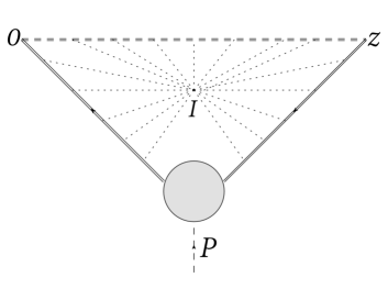
Figure 4: Star contribution at LO to the pion QPDA.

IV.2 QPDA and PDA at LO

IV.2.1 Zero mode contribution

The first contribution in (IV.1) can be readily evaluated in singular gauge. It is solely due to the zero modes. We note that for $k_{4}=0$ a pair of poles satisfying $k_{\perp}^{2}+x^{2}P_{z}^{2}=\frac{1}{4}E_{\pi}^{2}$ pinch the real $k_{4}$-integration line. To address the pinch, we rotate to Minkowski space $k_{4}\rightarrow ik_{4}$, shift $k_{4}\rightarrow k_{4}+(x-\frac{1}{2})P_{z}$ and carry the $k_{z}$-integration to have

$$\tilde{\phi}^{0}_{\pi}(x)\approx\lim_{P_{z}\rightarrow\infty}\frac{-4iN_{c}}{f^{2}_{\pi}}\int\frac{dk_{4}d^{2}k_{\perp}}{(2\pi)^{4}}\big{(}M(y_{1})M(y_{2})\big{)}^{\frac{1}{2}}\bigg{(}\frac{\bar{x}M(y_{1})+xM(y_{2})}{y_{1}^{2}y_{2}^{2}}\bigg{)}$$ (47)

with

$$y^{2}_{1}=-k_{4}(k_{4}+2xP_{z})+k_{\perp}^{2}-i\epsilon$$

$$y^{2}_{2}=-k_{4}(k_{4}-2\bar{x}P_{z})+k_{\perp}^{2}-i\epsilon$$ (48)

The integrand in (47) involves massless poles and also square-root branch points through the running mass (see below). The $k_{4}$-integration can be carried by contour integration. The poles are located at

$$k_{4\pm}=-xP_{z}\pm\sqrt{x^{2}P_{z}^{2}+k_{\perp}^{2}-i\epsilon}$$

$$\bar{k}_{4\pm}=+\bar{x}P_{z}\pm\sqrt{\bar{x}^{2}P_{z}^{2}+k_{\perp}^{2}-i\epsilon}$$ (49)

The pair $k_{4-},\bar{k}_{4+}$ moves to infinity at large momentum $P_{z}\rightarrow\infty$ and will be ignored (their contribution is exponentially small), while the pair

$$k_{4+}\approx\frac{k_{\perp}^{2}-i\epsilon}{2xP_{z}}$$

$$\bar{k}_{4-}\approx\frac{k_{\perp}^{2}-i\epsilon}{-2\bar{x}P_{z}}$$ (50)

approaches the real-axis, on opposite sides for $x\bar{x}\geq 0$ and the same sides for $x\bar{x}<0$. In the absence of the cuts, the QPDA has support only for $x\bar{x}\geq 0$ after pole closing. To proceed further, we need to address the cuts.

IV.2.2 Unmodified effective mass at large $P_{z}$

In singular gauge, the running mass $M(y_{1,2})$ at LO in (II.2) is given in terms of modified Bessel functions $I,K$ (A). When expressed in integral form, $I,K$ exhibit $({y^{2}_{1,2}})^{\frac{1}{2}}$ branch points. Note that the branch points are very explicit in regular gauge with (A)

$$M(y_{1,2})\approx e^{-2\rho(y^{2}_{1,2})^{\frac{1}{2}}}$$

We choose the branch-cut for the square-root function $({(a-k_{4})(b+k_{4})})^{\frac{1}{2}}$ to be along the negative imaginary axis such that at large $k_{4}>0$ the value of the square-root equals $-i$. The contour deformation of the $k_{4}$-integral into the upper half-plane, guarantees the positivity of the real part of $y_{1,2}$ and thus the decay of $M(y_{1,2})$ asymptotically. For $x\bar{x}>0$ the contribution from the poles is purely real, while for $x\bar{x}<0$ their contribution is complex. To ensure $x\leftrightarrow\bar{x}$ symmetry of the PDA after contour integration, the branch cuts have to be arranged symmetrically for the x- and $\bar{\rm x}$-contributions in (47). With this in mind, the result for the pion distribution amplitude (PDA) at LO is ($k_{\perp}\geq M(0)$)

$${\phi}^{0}_{\pi}(x)\approx\frac{2N_{c}M^{2}(0)}{f_{\pi}^{2}}\int\frac{d^{2}k_{\perp}}{(2\pi)^{3}}\frac{1}{k_{\perp}^{2}}\bigg{(}\theta(x\bar{x})\bigg{(}\bar{x}M_{\perp}^{\frac{1}{2}}+xM_{\underline{\perp}}^{\frac{1}{2}}\bigg{)}+\theta(-\bar{x})\,\bar{x}\,\bigg{(}M^{\frac{1}{2}}_{\perp}-\overline{M}^{\frac{3}{2}}_{\underline{\perp}}\bigg{)}+\theta(-x)\,x\,\bigg{(}M^{\frac{1}{2}}_{\underline{\perp}}-\overline{M}^{\frac{3}{2}}_{\perp}\bigg{)}\bigg{)}$$ (51)

with

$$M_{\perp}=\frac{M(k_{\perp}/\sqrt{x})}{M(0)}\,\qquad\,M_{\underline{\perp}}=\frac{M(k_{\perp}/\sqrt{\bar{x}})}{M(0)}\,\qquad\,\overline{M}_{\perp}=\frac{M(-ik_{\perp}/\sqrt{x})}{M(0)}\,\qquad\,\overline{M}_{\underline{\perp}}=\frac{M(-ik_{\perp}/\sqrt{\bar{x}})}{M(0)}$$ (52)

followed by the replacement $M(0)\rightarrow M(k)$ in the pion decay constant (32), to guarantee the normalization (46). In the physical region $x\bar{x}>0$, (51) can be evaluated in closed form since the integrand is a total derivative,

$${\phi}^{0}_{\pi}(x)\approx\frac{2N_{c}M^{2}(0)}{(2\pi)^{2}f_{\pi}^{2}}\left(\bar{x}F\left(\frac{\rho M(0)}{2\sqrt{x}}\right)+xF\left(\frac{\rho M(0)}{2\sqrt{\bar{x}}}\right)\right)\rightarrow\frac{1}{{\rm ln}\bigg{(}\frac{C}{\rho M(0)}\bigg{)}}\,\left(\bar{x}F\left(\frac{\rho M(0)}{2\sqrt{x}}\right)+xF\left(\frac{\rho M(0)}{2\sqrt{\bar{x}}}\right)\right)$$ (53)

The right-most relation follows from the leading logarithm approximation for the pion decay constant, with $\rho M(0)\sim\alpha$ and

$$F(z)\equiv I_{1}(z)K_{1}(z)-I_{0}(z)K_{0}(z)$$ (54)

The infrared sensitivity of the PDA follows from the enforcement of the power counting as we noted earlier. It matches the infrared sensitivity of the squared pion decay constant as given in (32), and cancels in the ratio after regulation $k_{\perp}\geq M(0)$ as we indicated earlier. To logarithmic accuracy, the PDA simplifies to

$$\phi_{\pi}^{0}(x)\rightarrow\theta(x\bar{x})$$ (55)

with support only in the physical range and unit normalization. In this deep infrared regime, the pion is composed democratically of partonic quarks in the range $0\leq x\leq 1$ including the end points.

For finite size instantons, the form factors $M_{\perp,\underline{\perp}}$ cause the PDA to vanish at the end points $x=0,1$ as initially noted in LAW1 , but otherwise develops spurious contributions in the non-physical region $x\bar{x}<0$ with real and imaginary parts. We recall that in the physical region with $x\bar{x}\geq 0$, the running mass involves a real combination of the modified Bessel functions $I,K$ as in (A), and a complex combination of the cylindrical Bessel functions $J,N$ for $x\bar{x}<0$ in the unphysical regions where momentum is conserved ($P_{z}=xP_{z}+\bar{x}P_{z}$) but energy is not ($|P_{z}|\neq|xP_{z}|+|\bar{x}P_{z}|$).

Current lattice simulations of the quasi-parton distributions LATTICE exhibit finite contributions outside the physically allowed x-support. However, they are vanishingly small at large momentum $P_{z}$. These spurious contributions relate to the transversality of the pion distribution in the QCD instanton vacuum. They do not arise in the $1/N_{c}$ analysis in two-dimensions QCD2 . We now show how to remove them approximately, without affecting the power counting in $\alpha$ at LO, and therefore gauge and chiral symmetry.

IV.2.3 Modified effective mass at large $P_{z}$

At large $P_{z}$, an approximative way to eliminate the spurious contributions without affecting the power counting in $\alpha$, is through the substitution $M(y)\rightarrow M(k_{\perp})$, which removes explicit $k_{4}$ dependence at the integrand level. It is cut-free and restricts the final $k_{\perp}$-integration to the expected physical range $M(0)\leq k_{\perp}\leq 1/\rho$. Unfortunately, this substitution fails at the end-points $x,\bar{x}=0$. To see this, we recall that for fixed $k_{\perp}$, the contribution to the QPDA follows from each of the two poles in (IV.2.1-IV.2.1) with at large $P_{z}$

$$\bigg{(}y_{1}^{2}=0:\,\,\,y_{2}^{2}=2k_{4}P_{z}\approx\frac{k_{\perp}^{2}}{x}\bigg{)}\qquad{\rm and}\qquad\bigg{(}y_{2}^{2}=0:\,\,\,y_{1}^{2}=-2k_{4}P_{z}\approx\frac{k_{\perp}^{2}}{\bar{x}}\bigg{)}$$ (56)

When a quark (antiquark) goes on mass shell the anti-quark (quark) virtuality becomes parametrically large at the end points $x,\bar{x}=0$. Say $x,\bar{x}\approx\alpha^{2}\ll 1$ at the end-points, then the $k_{\perp}$-integration range at each of the pole is vanishingly small with $M(0)\leq k_{\perp}\approx\alpha/\rho\approx M(0)$, causing the PDA to vanish. In contrast, when $x,\bar{x}\approx\alpha^{0}$ away from the end-points, the $k_{\perp}$-integration range is large with $M(0)\leq k_{\perp}\leq 1/\rho$ in line with the leading logarithmic approximation and power counting in (53).

A simple modification of the induced effective quark mass (13) at large $P_{z}$, that enforces these observations without upsetting the power counting in $\alpha$, that is commensurate with (56) with manifest $x\leftrightarrow\bar{x}$ symmetry and free of spurious contributions, is

$$M(y)\rightarrow M\bigg{(}\frac{k_{\perp}}{\lambda_{\pi}\sqrt{|x\bar{x}|}}\bigg{)}=M(0)\bigg{(}\left|z\left(I_{0}K_{0}-I_{1}K_{1}\right)^{\prime}\right|^{2}\bigg{)}_{z=\frac{\rho k_{\perp}}{2\lambda_{\pi}\sqrt{|x\bar{x}|}}}\equiv M(0)\bigg{(}\left|zF^{\prime}(z)\right|^{2}\bigg{)}_{z=\frac{\rho k_{\perp}}{2\lambda_{\pi}\sqrt{|x\bar{x}|}}}$$ (57)

where $\lambda_{\pi}\approx\alpha^{0}$ is a parameter of order 1, which is fixed by normalizing the PDA. We note that the PDA is normalized in power counting at LO for the unmodified effective mass. With this in mind, the closed-form PDA at LO following from the large $P_{z}$ limit is ($k_{\perp}\geq M(0)$)

$$\phi^{0}_{\pi}(x)\rightarrow\frac{2N_{c}}{f_{\pi}^{2}}\int\frac{d^{2}k_{\perp}}{(2\pi)^{3}}\frac{\theta(x\bar{x})}{k_{\perp}^{2}}{M^{2}(k_{\perp}/\lambda_{\pi}\sqrt{x\bar{x}})}\rightarrow\frac{\theta(x\bar{x})}{{\rm ln}\bigg{(}\frac{C}{\rho M(0)}\bigg{)}}\int_{\rho M(0)/2\lambda\sqrt{x\bar{x}}}^{\infty}dz\,z^{3}F^{\prime\,4}(z)$$ (58)

(58) is similar to (53), but with no spurious contributions! For $x,\bar{x}\approx\alpha^{2}$, the effective quark mass in (58) is probed at virtualities larger than $1/\rho$, which is still justified by noting the agreement of the effective quark mass with the lattice data at large momenta in Fig. 2.

IV.2.4 Non-zero mode contribution

The non-zero mode contributions in (IV.1) do not vanish at finite $P_{z}$, but are in general small due to the fact that at short distances $G_{I}\approx S_{0}$ or $\delta G_{I}\approx 0$ (UV limit), a standard approximation in the random instanton model. For an estimate of their contribution beyond, we may use the Born approximation (III.4) in (IV.1). A close inspection shows that the ensuing color-spin traces are short of the binary pole structure $1/(y_{1}^{2}y_{2}^{2})$ which is required for: 1/ a finite contribution as $P_{z}\rightarrow\infty$; 2/ a finite contribution for $x\bar{x}\geq 0$. In this approximation, the non-zero modes do not contribute to the PDA as $P_{z}\rightarrow\infty$.

A more explicit evaluation of the non-zero modes in (IV.1) follows from the observation that after analytical continuation the external quark lines are put on mass-shell. The ensuing contribution to (IV.1) can be worked out in closed form. Using the modified cutoff, and the definitions of the mass-shell conditions in Appendix E, a lengthy calculation gives

$$\phi_{\pi}^{\not{0}}(x)\approx\lim_{P_{z}\rightarrow\infty}\frac{\alpha}{f_{\pi}^{2}}\frac{(\sqrt{2}\pi\rho)^{2}}{\sigma_{00}P_{z}}\int\frac{d^{2}k_{\perp}}{(2\pi)^{3}}{M(k_{\perp}/\lambda_{\pi}\sqrt{x\bar{x}})}\,{\rm Tr}\bigg{(}{\sigma}^{z}\bigg{(}\bigg{(}\overline{\mathbb{F}}(P,k_{2})-\overline{\mathbb{F}}(P,k_{1})\bigg{)}-\bigg{(}\mathbb{F}(P,k_{2})-\mathbb{F}(P,k_{1})\bigg{)}\bigg{)}\bigg{)}$$ (59)

Here $k_{1,2}=k\pm P/2$ with $k_{1,2}^{2}\approx 0$ in the large $P_{z}$ limit and $P^{2}=0$ on mass shell. The first contribution is from the instanton and the second contribution from the anti-instanton in the bracket. The form factors are

$$\mathbb{F}(P,p)=\frac{\sigma_{z}\overline{p}+p\sigma_{z}}{2p\cdot P}\,f(\rho\sqrt{P^{2}})+\bigg{(}\frac{\sigma_{z}(\overline{P}+\overline{p})+(P+p)\sigma_{z}}{(P+p)^{2}}-\frac{\sigma_{z}\overline{p}+p\sigma_{z}}{2p\cdot P}\bigg{)}\,f(\rho\sqrt{(p+P)^{2}})$$

$$\overline{\mathbb{F}}(P,p)=\frac{\sigma_{z}{p}+\overline{p}\sigma_{z}}{2p\cdot P}\,f(\rho\sqrt{P^{2}})+\bigg{(}\frac{\sigma_{z}(P+p)+(\overline{P}+\overline{p})\sigma_{z}}{(\overline{P}+\overline{p})^{2}}-\frac{\sigma_{z}p+\overline{p}\sigma_{z}}{2p\cdot P}\bigg{)}\,f(\rho\sqrt{(p+P)^{2}})$$ (60)

with $f(z)=zK_{1}(z)-1$. Throughout, the Weyl notation $p=p_{\mu}\sigma^{\mu}$, $\overline{p}=p_{\mu}\overline{\sigma}^{\mu}$ etc. is used with $\sigma^{\mu}=(1,\vec{\sigma})$ and $\overline{\sigma}^{\mu}=(1,-\vec{\sigma})$. The finite contribution in (IV.2.4) when inserted in (59) cancels out. The non-zero mode contribution (59) to the PDA vanishes at LO.

IV.2.5 Massive Pion and Kaon

The explicit breaking of chiral symmetry by light quark masses $u,d,s$ is understood in the QCD instanton vacuum, with the masses for the pion and kaon in LO obeying the GOR relation DP ; IQCD ; MF . In our case, this can be explicitly checked to hold in power counting. For a finite current mass $m$, a rerun of the arguments leading to the effective quark mass in (II.2) yields

$$M(p,m)=\frac{\alpha\,|p\varphi^{\prime}(p)|^{2}}{\bigg{(}2||q\varphi^{\prime 2}||^{2}+\frac{m^{2}}{4\alpha^{2}}\bigg{)}^{\frac{1}{2}}+\frac{m}{2\alpha}}+m\equiv\frac{M(p,0)}{\bigg{(}1+\xi^{2}\bigg{)}^{\frac{1}{2}}+\xi}+m$$ (61)

with the mass parameter

$$\xi=\frac{mM(0,0)\rho^{2}}{8\pi^{2}\kappa}$$ (62)

For light quarks $M(0)\equiv M(0,0)\approx 386$ MeV and $\rho\approx 1/(631{\rm MeV})$. For massive quarks we find $M(0,5)\approx 383.7\,\textrm{MeV}\approx M(0)$ and $M(0,150)\approx 372.6\,\textrm{MeV}\approx M(0)$ for the up-down and strange quarks respectively. The effective quark mass is almost unchanged. As a result, the pseudoscalar decay constant for the pion and kaon are about the same at LO for massive quarks.

For the massive case, the integral equation (25) for the pseudoscalar meson vertex holds with the substitution

$$\sigma_{00}\rightarrow{\bigg{(}2||q\varphi^{\prime 2}||^{2}+\frac{m^{2}}{4\alpha^{2}}\bigg{)}^{\frac{1}{2}}+\frac{m}{2\alpha}}\approx\sqrt{2}||q\varphi^{\prime 2}||+\frac{m}{2\alpha}$$ (63)

As a result the mass-shell vertex (III.2) at LO changes to

$$\bigg{(}iO_{5}(P,k)\bigg{)}_{P^{2}\approx-m_{P}^{2}}\approx\frac{\sqrt{N_{c}}}{f_{P}}\sqrt{M(k)}\left(\frac{i\gamma_{5}}{P^{2}+m_{P}^{2}}\right)\sqrt{M(k-P)}$$ (64)

with $f_{P}\approx f_{\pi}$ and $m_{P}^{2}\approx i2m\left<\psi^{\dagger}\psi\right>$ as expected. Note that in (64) both $f_{P}$ and $M(k)$ are found to be unaffected by the current mass $m$ at the meson pole at LO. The latter only shifts the meson pole in agreement with the GOR relation.

The ensuing PDA for massive pseudoscalars simplifies to LO

$$\phi^{0}_{P}(x)\approx \frac{2N_{c}M^{2}(0)}{f_{P}^{2}}\int\frac{d^{2}k_{\perp}}{(2\pi)^{3}}\frac{1}{k_{\perp}^{2}-x\bar{x}m_{P}^{2}}$$

$$\times\bigg{(}\theta(x\bar{x})\bigg{(}\bar{x}M_{\perp}+xM_{\underline{\perp}}\bigg{)}+\theta(-\bar{x})\,\bar{x}\,\bigg{(}M_{\perp}-M_{\underline{\perp}}\bigg{)}+\theta(-x)\,x\,\bigg{(}M_{\underline{\perp}}-M_{\perp}\bigg{)}\bigg{)}$$

with the same cutoff $k_{\perp}\geq M(0)$ for light quarks $u,d,s$. For comparison, the result for the modified effective quark mass (57) is

$$\phi^{0}_{P}(x)\rightarrow\frac{2N_{c}}{f_{P}^{2}}\int\frac{d^{2}k_{\perp}}{(2\pi)^{3}}\frac{\theta(x\bar{x})}{k_{\perp}^{2}-x\bar{x}m_{P}^{2}}{M^{2}(k_{\perp}/\lambda_{P}\sqrt{x\bar{x}})}$$ (66)

In Fig. 5 we show the pion PDA (66) at LO for varying $\rho$ but fixed $M(0)=386$ MeV (solid curves) in comparison to the asymptotic result of $6x\bar{x}$ AS (dashed curve). We have set $f_{\pi}=93$ MeV and $m_{\pi}=135\,\textrm{MeV}$ and fixed $\lambda_{\pi}=3.41894$ for the overall normalization of the PDA with the modified effective mass. (No such a modification is needed for the unmodified effective quark mass). The result at this low renormalization scale $Q_{0}=1/\rho$ is remarkably close to the QCD asymptotic result of $6x\bar{x}$ AS . The single $q\bar{q}$-component of the pion wavefunction is well described in the random instanton vacuum (RIV) in the planar approximation at LO. Since the constituent mass $M(0)\approx M(0,5)\approx M(0,150)$ is almost unchanged for $u,d,s$, the kaon PDA is almost undistinguishable from the pion PDA at LO.

Our result for the pion PDA at LO is similar to the one obtained originally in LAW1 using time-like arguments with a modified dipole effective quark mass with very different analytical properties. It is overall analogous to the one derived from modified holographic models BROD . As $\rho\rightarrow 0$, and the cutoff is removed, the pion PDA asymptotes the middle-solid-red curve in Fig. 5 which is close to the normalized step function $\theta(x\bar{x})$. The same result was noted for chiral quark models with point interactions BASIS ; BRO , and some bound-state resummations M3 .

In Fig. 6 we compare our result for the pion PDA shown in red-solid line (RIV) to the recently generated pion PDA blue-wide-band, using lattice simulations using the large momentum effective theory (LaMET) JI . The QCD asymptotic result black-dashed curve is again shown for comparison.

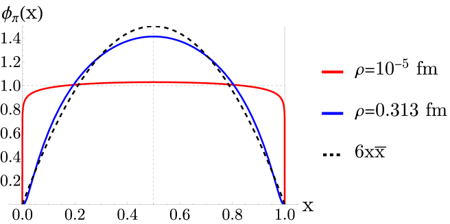
Figure 5: Pion PDA (66) for varying instanton size $\rho$ but fixed $M(0)=386$ MeV (solid curves) in comparison to the asymptotic result of $6x\bar{x}$ AS (dashed curve).

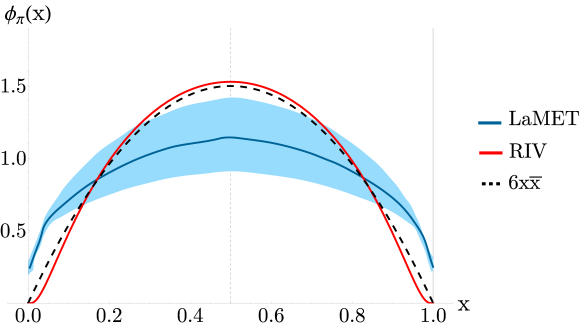
Figure 6: Pion PDA from the random instanton model (RIV, solid-red-curve) (66), asymptotic QCD (dashed-black-curve) AS in comparison to the lattice simulations LaMET (blue-wide-band) JI

.

IV.3 QCD evolution of pion PDA

The pion PDA (66) is defined at a low renormalization scale set by the instanton size $Q_{0}=1/\rho=631$ GeV. Assuming factorization, its form at higher renormalization scales follows from a QCD kernel evolution equation (ERBL). Its closed form solution in the form of Gegenbauer polynomials was given in AS . More specifically, using (58) as an initial condition, the ERBL evolved pion PDA is AS

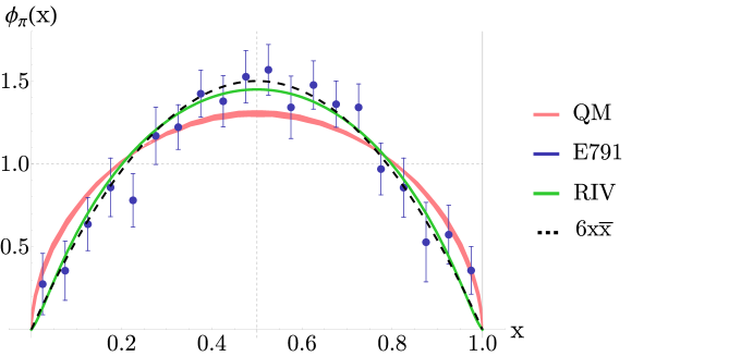
Figure 7: Pion PDA from the random instanton model evolved to $Q=2\,\textrm{GeV}$ (RIV, solid-red-curve) (58), the quark model QM@2GeV (QM, solid-pink-band) BRO , asymptotic QCD (dashed-black-curve) AS in comparison to the E791 dijet data E791

.

$$\phi_{\pi}(x,Q)=6x\bar{x}\sum_{n-even}a_{n}(Q_{0})\bigg{(}\frac{\alpha_{s}(Q)}{\alpha_{s}(Q_{0})}\bigg{)}^{\gamma_{n}/\beta_{0}}\,C_{n}^{\frac{3}{2}}(x-\bar{x})$$ (67)

with the initial coefficients

$$a_{n}(Q_{0})=\frac{2(2n+3)}{3(n+1)(n+2)}\int_{0}^{1}dy\,C_{n}^{\frac{3}{2}}(y-\bar{y})\,\phi^{0}_{\pi}(y)$$ (68)

Here $\alpha_{s}(Q)=4\pi/\beta_{0}{\rm ln}(Q^{2}/\Lambda^{2})$ is the one-loop running QCD coupling with $\beta_{0}=\frac{11}{3}N_{c}-\frac{2}{3}N_{f}$ and $\Lambda=250$ MeV ($\overline{\rm MS}$-scheme). The $\gamma_{n}$ are pertinent anomalous dimensions

$$\gamma_{n}=C_{F}\bigg{(}1+4\sum_{k=2}^{n+1}\frac{1}{k}-\frac{2}{(n+1)(n+2)}\bigg{)}$$ (69)

with the Casimir $C_{F}=(N_{c}^{2}-1)/2N_{c}$. Since $\gamma_{0}=1$ and $\gamma_{n}>0$, it follows that (67) asymptotes $6x\bar{x}$ with $a_{0}(Q_{0})=1$ for $Q\rightarrow\infty$ as illustrated in Fig. 5.

In Fig. 7 we show the ERBL evolved pion PDA (58) at $Q=2$ GeV as a green-solid curve (RIV), which is in good agreement with the empirical pion PDA blue-data points extracted from dijet data by the E791 collaboration E791 at the same scale. For comparison, we also show the chiral quark model evolved PDA to $Q=2$ GeV as a solid-pink-band (QM) BRO and the asymptotic QCD result AS . Again, since $M(0)$ does not change much for massive pions and kaons, the ERBL evolved kaon PDA is undistinguishable from its evolved pion counterpart at LO in the present analysis.

V Pion quasi-parton distribution function

In this section we show how to re-sum the planar contributions to the three-point functions in general. We then apply the results to the derivation of the pion quasi-parton distribution function to LO. Since this distribution obeys charge and momentum sum rules, the enforcement of the gauge and chiral symmetry through the Ward identity is needed.

V.1 Three-point function

The quasi-parton distributions involve 3-point functions with one of the source point-split. In the planar approximation, their construction follows a similar reasoning as the one developed earlier. For that, consider the general 3-point function

$$\left<O_{1}O_{3}O_{2}\right>$$ (70)

where the $O^{\prime}$s are resummed and colorless local or quasi-local fermionic bilinears defined as

$$O_{ab}={\rm Tr}_{C}\left(S_{\gamma\beta}O_{\beta\alpha}S_{\alpha\delta}T_{a\gamma;\delta b}\right)$$ (71)

and are spin-flavor valued in general. In the planar approximation, the leading contributions to (70) are

$$\left<O_{1}O_{3}O_{2}\right>={\rm Tr}_{C}(O_{3}SO_{2}SO_{1}S)+\frac{N}{2N_{c}V}\int_{I+\bar{I}}dz_{I}{\rm Tr}_{C}\left(O_{3}S(-\Sigma_{I})SO_{2}S(-\Sigma_{I})SO_{1}S(-\Sigma_{I})S\right)$$ (72)

The first contribution sums up all planar diagrams with no common instanton to the three quark lines as illustrated in Fig. 8. The second contribution corresponds to the planar contributions with one instanton shared by the three quark lines. Planarity implies that only one instanton is commonly shared by the three quark lines as shown in Fig. 9. For a finite gauge link $[z_{-},z_{+}]$ there is an additional contribution shown in Fig. 10 with $I,J$ referring to a double summation over distinct instantons (anti-instantons). It is readily seen that this contribution reduces to that shown in Fig. 9 when the gauge link is 1, so it will be ignored. The direct and cross contributions follow from pertinent re-routing of the momenta. The extension of these observations to the $n$-point functions is now straightforward.

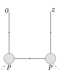
Figure 8: Tree contribution at LO to the pion QPDF

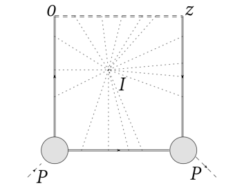
Figure 9: Star contribution at LO to the pion QPDF

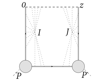
Figure 10: Split contribution at LO to the pion QPDF

V.2 Pion QPDF and PDF at LO

The pion quasi-distribution function (QPDF) can also be extracted from the equal-time correlator following (1) as suggested in JI1 . In our case it follows by reduction using the pseudoscalar source. Specifically, in the chiral limit we have

$$\tilde{\psi}_{\pi}(x,P_{z})=\int\frac{dz}{2\pi}\,e^{-\frac{i}{2}(x-\bar{x})zP_{z}}\,\left<\pi(P)\right|{\psi}^{\dagger}(z_{-})\gamma^{z}\,[z_{-},z_{+}]\psi(z_{+})\left|\pi(P)\right>$$

$$\approx\lim_{P^{2}\rightarrow 0}\frac{P^{4}}{g_{\pi}^{2}}\int\frac{dz}{2\pi}\,e^{-\frac{i}{2}(x-\bar{x})zP_{z}}\,\left<O_{5}(-P){\psi}^{\dagger}(z_{-})\gamma^{z}\,[z_{-},z_{+}]\,\psi(z_{+})O_{5}(P)\right>$$

Following the previous reasoning we may approximate the gauge link to 1 in the large $P_{z}$ limit. Using the density expansion for the pseudoscalar vertex (34) and the effective mass (16) at NLO, we can unwind (V.2). The result at LO

$$\tilde{\psi}_{\pi}(x,P_{z})\approx$$

$$-\lim_{P^{2}\rightarrow 0}\frac{P^{4}}{g_{\pi}^{2}P_{z}}\int\frac{d^{4}k}{(2\pi)^{4}}\delta\left(x-\frac{1}{2}-\frac{k_{z}}{P_{z}}\right){\rm Tr}_{C}\bigg{(}\gamma^{z}\frac{1}{\not{k}_{1}}\gamma^{5}F_{5}(P,k)\frac{1}{\not{k}_{2}}\gamma^{5}F_{5}(P,k)\frac{1}{\not{k}_{1}}\bigg{)}+{\rm cross}$$

$$+\lim_{P^{2}\rightarrow 0}\frac{P^{4}}{g_{\pi}^{2}\sigma_{00}^{2}P_{z}}\int\frac{d^{4}k}{(2\pi)^{4}}\frac{d^{4}q}{(2\pi)^{4}}\frac{d^{4}p}{(2\pi)^{4}}\delta\left(x-\frac{1}{2}-\frac{k_{z}}{P_{z}}\right){\rm Tr}_{C}\bigg{(}\gamma^{z}\psi_{0I}(k_{1})\psi_{0I}^{\dagger}(q_{1})\gamma^{5}F_{5}(P,q)\delta G_{I}(q_{2},p_{2})\gamma^{5}F_{5}(P,p)\psi_{0I}(p_{1})\psi_{0I}^{\dagger}(k_{1})\bigg{)}$$

$$+\lim_{P^{2}\rightarrow 0}\frac{P^{4}}{g_{\pi}^{2}\sigma_{00}^{2}P_{z}}\int\frac{d^{4}k}{(2\pi)^{4}}\frac{d^{4}q}{(2\pi)^{4}}\frac{d^{4}p}{(2\pi)^{4}}\delta\left(x-\frac{1}{2}-\frac{k_{z}}{P_{z}}\right){\rm Tr}_{C}\bigg{(}\gamma^{z}\psi_{0I}(k_{1})\psi_{0I}^{\dagger}(q_{1})\gamma^{5}F_{5}(P,q)\psi_{0I}(q_{1})\psi_{0I}^{\dagger}(p_{2})\gamma^{5}F_{5}(P,p)\delta G_{I}(p_{1},k_{1})\bigg{)}$$

$$+\lim_{P^{2}\rightarrow 0}\frac{P^{4}}{g_{\pi}^{2}\sigma_{00}^{2}P_{z}}\int\frac{d^{4}k}{(2\pi)^{4}}\frac{d^{4}q}{(2\pi)^{4}}\frac{d^{4}p}{(2\pi)^{4}}\delta\left(x-\frac{1}{2}-\frac{k_{z}}{P_{z}}\right){\rm Tr}_{C}\bigg{(}\gamma^{z}\delta G_{I}(k_{1},q_{1})\gamma^{5}F_{5}(P,q)\psi_{0I}(q_{2})\psi_{0I}^{\dagger}(p_{2})\gamma^{5}F_{5}(P,p)\psi_{0I}(p_{1})\psi_{0I}^{\dagger}(k_{1})\bigg{)}$$

with $k_{1,2}=k\pm\frac{P}{2}$ and so on. The summation over $I,\bar{I}$ is subsumed. The cross refers to the cross contributions (see below). All contributions are of order $\alpha^{0}$ since $g_{\pi}\sim\alpha^{0}$ and $\sigma_{00}\sim\alpha^{0}$. The first contribution involves only the zero modes. The second to fourth contributions involve the cross contribution from the zero and non-zero modes. The latters are required for the enforcement of the Ward identities in power counting, and all contributions are of the same order in $\alpha$. We note that the second contribution in (V.2) vanishes due to a mismatch in chirality.

V.2.1 Non-zero mode contribution

An explicit evaluation of the non-zero modes in (V.2) is involved, but follows from the observation that after analytical continuation the external quark lines are put on mass-shell as we noted earlier for the PDA. In Appendix E the rules for putting the instanton zero modes and non-zero mode propagator on mass shell are given. The ensuing contribution to (V.2) can be worked out in closed form much like for the PDA. Using the modified cutoff, a lengthy calculation gives

$$\psi_{\pi}^{\not{0}}(x)\approx\lim_{P_{z}\rightarrow\infty}\frac{(\sqrt{2}\pi\rho)^{2}}{f_{\pi}^{2}\sigma_{00}^{2}P_{z}}\int\frac{d^{2}k_{\perp}}{(2\pi)^{3}}{M^{2}(k_{\perp}/\lambda_{\pi}\sqrt{x\bar{x}})}\,{\rm Tr}\bigg{(}{\sigma}^{z}\bigg{(}2{\mathbb{F}}(0,k_{1})+2\overline{\mathbb{F}}(0,k_{1})\bigg{)}$$ (75)

with $k_{1}=k+P/2$ and $k_{1}^{2}\approx 0$ at large $P_{z}$. The form factors are given in (IV.2.4). They are zero for the present kinematics. The non-zero mode contribution (75) vanishes. So in the large momentum limit the pion PDF at LO is dominated by the zero mode contribution which we now explicit.

V.2.2 Pion and Kaon PDF at LO and large $P_{z}$

The first contribution in (V.2) is dominated by the pion pole. Inserting (25), carrying the spin trace, unwinding the $k_{z}$-integration and analytically continuing $k_{4}\rightarrow ik_{4}$ yield ($k_{\perp}\geq M(0)$)

$$\tilde{\psi}^{0}_{\pi}(x,P_{z})\approx\frac{4iN_{c}}{f_{\pi}^{2}}\int\frac{dk_{4}d^{2}k_{\perp}}{(2\pi)^{4}}\,\bigg{(}M(y_{1})M(y_{2})\bigg{(}\frac{x+\bar{x}}{y_{1}^{2}y_{2}^{2}}+\frac{x}{y_{1}^{4}}\bigg{)}+M(y_{1})M(y^{\prime}_{2})\bigg{(}-\frac{x+\bar{x}}{y_{1}^{2}(y^{\prime}_{2})^{2}}+\frac{x}{y_{1}^{4}}\bigg{)}\bigg{)}$$ (76)

with $y_{1,2}$ given in (IV.2.1), and $y^{\prime}_{2}=k+P$ in the cross contribution. (76) can be undone by pole closing. In the large $P_{z}$ limit, the cross contribution in (76) and the contribution $1/y_{1}^{4}$ in (76) are subleading. Using the unmodified effective quark mass (13), the result for the pion PDF at LO and large $P_{z}$ and in the chiral limit is

$$\psi^{0}_{\pi}(x)\approx\frac{2N_{c}M^{2}(0)}{f_{\pi}^{2}}\int\frac{d^{2}k_{\perp}}{(2\pi)^{3}}\frac{1}{k_{\perp}^{2}}\bigg{(}\theta(x\bar{x})\bigg{(}\bar{x}M_{\perp}+xM_{\underline{\perp}}\bigg{)}+\theta(-\bar{x})\,\bar{x}\,\bigg{(}M_{\perp}-M_{\underline{\perp}}\bigg{)}+\theta(-x)\,x\,\bigg{(}M_{\underline{\perp}}-M_{\perp}\bigg{)}\bigg{)}$$

Note that a similar conclusion follows from the free approximation for the non-zero modes $\delta G_{I}\approx 0$, or the Born approximation (III.4). For comparison, the result with the modified effecttive quark mass (57) is

$$\psi^{0}_{\pi}(x)\rightarrow\frac{2N_{c}}{f_{\pi}^{2}}\int\frac{d^{2}k_{\perp}}{(2\pi)^{3}}\frac{\theta(x\bar{x})}{k_{\perp}^{2}}{M^{2}(k_{\perp}/\lambda_{\pi}\sqrt{x\bar{x}})}\approx\phi_{\pi}^{0}(x)$$ (78)

Away from the chiral limit, the QPDF involve several contributions that will be presented elsewhere. We have checked that the PDF limit at LO simplifies. For the unmodified quark effective mass (13) the PDF for the f-flavor in the the P-pseudoscalar or $f/P$ is

$$\psi^{0}_{f/P}(x)\approx\frac{2N_{c}M^{2}(0)}{f_{P}^{2}}\int_{f}\frac{d^{2}k_{\perp}}{(2\pi)^{3}}\frac{k_{\perp}^{2}}{(k_{\perp}^{2}-x\bar{x}m_{P}^{2})^{2}}\bigg{(}\theta(x\bar{x})\bigg{(}\bar{x}M_{\perp}+xM_{\underline{\perp}}\bigg{)}+\theta(-\bar{x})\,\bar{x}\,\bigg{(}M_{\perp}-M_{\underline{\perp}}\bigg{)}+\theta(-x)\,x\,\bigg{(}M_{\underline{\perp}}-M_{\perp}\bigg{)}\bigg{)}$$

while for the modified quark effective mass (57) it is

$$\psi^{0}_{f/P}(x)\rightarrow\frac{2N_{c}}{f_{P}^{2}}\int_{f}\frac{d^{2}k_{\perp}}{(2\pi)^{3}}\frac{\theta(x\bar{x})\,k_{\perp}^{2}}{(k_{\perp}^{2}-x\bar{x}m_{P}^{2})^{2}}{M^{2}(k_{\perp}/\lambda_{P}\sqrt{x\bar{x}})}$$ (80)

The $f$-integration is carried with $k_{\perp}\geq M(0,m_{f})$, with $f=u,d$ for the pion and $f=u,s$ for the kaon.

V.3 QCD evolution of pion and kaon PDF

To compare the pion and kaon PDF in the random instanton vacuum at the inverse instaon size scale $Q_{0}=1/\rho=631$ GeV, with the measured pion PDF at higher resolution we need to evolve the pion PDF (80) to a higher scale using QCD evolution (DGLAP). A more appropriate evolution with a modified DGLAP kernel including small size instanton corrections will be discussed elsewhere. With this in mind, the one-loop DGLAP evolution of the forward (non-singlet) pseudoscalar PDF $\psi_{P}(x,t)$ is

$$\frac{d\psi_{P}(x,t)}{dt}=\frac{\alpha_{s}(t)}{2\pi}\int_{x}^{1}\frac{dy}{y}P_{qq}^{(0)}\left(\frac{x}{y}\right)\psi_{P}(y,t)$$ (81)

with $t=\log(Q^{2}/\Lambda_{\textrm{QCD}}^{2})$ and $P_{qq}^{(0)}(z)$ is the one-loop non-singlet splitting function

$$P_{qq}^{(0)}(z)=C_{F}\left[\frac{1+z^{2}}{(1-z)_{+}}+\frac{3}{2}\delta(1-z)\right]$$ (82)

We numerically evolve from $t$ to $t+\Delta t$ by simple forward-Euler. We sample $\psi_{P}(x,t)$ on a uniform grid in $x$, create a spline-interpolation, and evaluate the RHS of (81) to calculate $d\psi$. Consistency of the evolution is checked in two ways: first by verifying that the first few Mellin moments evolve according to the analytical result

$$M_{n}(t)\equiv\int_{0}^{1}x^{n}\psi_{P}(x,t)\,dx=M(t_{0})\left(\frac{\alpha_{s}(t)}{\alpha_{s}(t_{0})}\right)^{\gamma_{n}/\beta_{0}}$$ (83)

where $\gamma_{n}$ is the same as before in (69), and second by we reproducing the evolution of BRO where the authors evolve a step-function $\psi_{P}(x,t_{0})=\theta(x\bar{x})$ from $Q_{0}=313\,\textrm{MeV}$ to $Q=2\,\textrm{GeV}$ with $\Lambda_{\textrm{QCD}}=226\,\textrm{MeV}$.

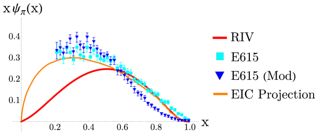
Figure 11: Pion longitudinal momentum distribution in the QCD instanton vacuum RIV solid-red-curve (V.2.2), the E615 data blue-square E615 and improved E615 data inverse-blue-triangle E615MOD , and the EIC projection in solid-orange-curve EICPRO . All are evolved to $Q^{2}=4\textrm{GeV}^{2}$.

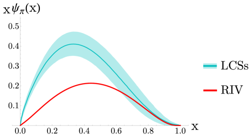
Figure 12: Pion longitudinal momentum distribution in the QCD instanton vacuum evolved to $Q^{2}=27\,\textrm{GeV}^{2}$ (RIV, solid-red-curve) (V.2.2) in comparison to the lattice results LCSs blue-wide-band at the same scale LCS .

In Fig. 11 we show the result for the pion longitudinal momentum distribution in our QCD random instanton vacuum (RIV) in solid-red-curve (V.2.2) evolved to $Q^{2}=4$ GeV². The data are from the E615 collaboration blue-square E615 , and the improved E615 data inverse-blue-triangle E615MOD . The EIC projection is shown in solid-orange-curve EICPRO . All are evolved to the same $Q^{2}=4\textrm{GeV}^{2}$. In Fig. 12 we show the pion longitudinal distribution in the QCD random instanton vacuum (RIV) solid-red-curve in comparison to recent lattice results (LCSs) as a blue-wide-band LCS at a higher scale $Q^{2}=27$ GeV². There is good agreement at large-x, but the RIV results fall short at low-x. This maybe a shortcoming of our planar approximation which ignores multi-$q\overline{q}$ or sea contributions to the pion wavefunction at low-x. We note that for smaller size instantons, the pion (kaon) PDF shown in Fig. 5 flatens out. Its DGLAP evolution is more in line with the data for all-x. However, smaller size instantons do not support the key vacuum parameters we have established earlier.

V.4 Pion TMD at LO and large $P_{z}$

Finally, we note that the integrand in (80) describes the parton transverse momentum distribution (TMD) in a pseudoscalar $P$. However at this point we must recall (23) — that our actual leading-order TMD is only obtained after shifting back $k_{\perp}^{2}\rightarrow k_{\perp}^{2}+M^{2}(0)$. It follows that the TMD for the massive pion at LO is

$$\psi^{0}_{\pi}(x,k_{\perp})\rightarrow\frac{2N_{c}}{f_{\pi}^{2}}\frac{1}{(2\pi)^{3}}\,\frac{\theta(x\bar{x})\,(k_{\perp}^{2}+M^{2}(0))}{(k_{\perp}^{2}+M^{2}(0)-\bar{x}xm_{\pi}^{2})^{2}}{M^{2}\left(\frac{\sqrt{k_{\perp}^{2}+M^{2}(0)}}{\lambda_{\pi}\sqrt{x\bar{x}}}\right)}$$ (84)

while the transverse spatial distribution is

$$\psi^{0}_{\pi}(x,b_{\perp})\rightarrow\frac{2N_{c}}{f_{\pi}^{2}}\int\frac{d^{2}k_{\perp}}{(2\pi)^{3}}\,e^{ik_{\perp}\cdot b_{\perp}}\,\frac{\theta(x\bar{x})\,k_{\perp}^{2}}{(k_{\perp}^{2}-\bar{x}xm_{\pi}^{2})^{2}}{M^{2}(k_{\perp}/\lambda_{\pi}\sqrt{x\bar{x}})}$$ (85)

with $k_{\perp}\geq M(0)$ subsumed. The leading logarithm contribution to the TMD in the massless case is

$$\psi^{0}_{\pi}(x,b_{\perp})\rightarrow\frac{\theta(x\bar{x})}{4{\rm ln}\bigg{(}\frac{C}{\rho M(0)}\bigg{)}}\int_{\rho M(0)/2\lambda_{\pi}\sqrt{x\bar{x}}}^{\infty}dz\,J_{0}\bigg{(}2\sqrt{x\bar{x}}\frac{zb_{\perp}}{\rho}\bigg{)}\,z^{3}F^{\prime\,4}(z)$$ (86)

For comparison, the massless pion TMD with the unmodified effective quark mass (13) in the physical region $x\bar{x}\geq 0$, is

$$\psi^{0}_{\pi}(x,b_{\perp})\approx\frac{N_{c}\rho^{2}M^{2}(0)}{2f_{\pi}^{2}}\int_{M(0)}^{\infty}\frac{k_{\perp}dk_{\perp}}{(2\pi)^{2}}\,J_{0}(k_{\perp}b_{\perp})\bigg{(}\frac{\overline{x}}{x}\,F^{\prime\,2}\bigg{(}{z}_{k}=\frac{\rho k_{\perp}}{2\sqrt{x}}\bigg{)}+\frac{{x}}{\overline{x}}\,F^{\prime\,2}\bigg{(}\overline{z}_{k}=\frac{\rho k_{\perp}}{2\sqrt{\overline{x}}}\bigg{)}\bigg{)}$$ (87)

with $F^{\prime}(z)$ the z-derivative of (54).

In Fig. 13 we show the pion and kaon transverse spatial distributions from the QCD random instanton vacuum (87), at the low renormalization scale $Q_{0}=631\,\textrm{MeV}$. The corresponding distributions in transverse momentum space are also shown in Fig. 14 at the same scale.

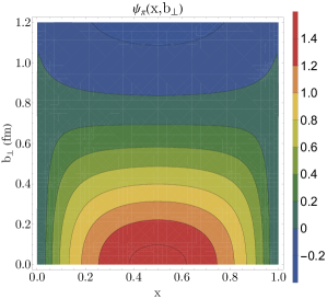
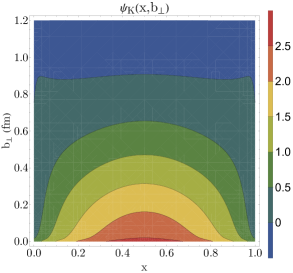
Figure 13: Pion and Kaon transverse spatial distribution from the QCD instanton vacuum (87) with physical masses and at renormalization scale $Q_{0}=631\,\textrm{MeV}$.

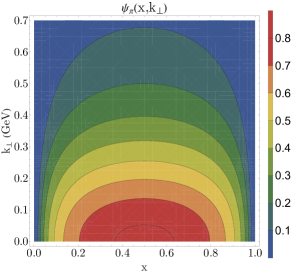
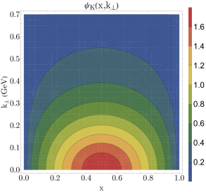
Figure 14: Pion and Kaon transverse momentum distribution from the QCD instanton vacuum (87) with physical masses and at renormalization scale $Q_{0}=631\,\textrm{MeV}$.

VI Conclusions

We revisited the QCD instanton vacuum in the context of an exact planar re-summation of the n-point correlations that preserves both gauge and chiral symmetry in power counting using the root of the packing fraction $\alpha\approx\sqrt{\kappa}$. We analysed the induced quark mass, effective pion pseudo-scalar and pseudo-vector vertices at NLO with full conformity with the axial Ward identity in the chiral limit. NNLO contributions are readily available but tedious.

We used this framework to derive the soft contributions to the pion and kaon QPDA, QPDF and QGPDF following from the QCD instanton vacuum. The results in LO show that these pion quasi-distributions receive contributions from both the zero modes and the non-zero modes, but the latters drop out in the large momentum limit from the PDA, PDF and TMD. They are made explicit at LO or leading logarithm approximation.

The results we presented for the pion and kaon partonic distributions are all evaluated at the low renormalization scale set by the inverse instanton size $1/\rho=631$ MeV. A more compelling comparison with data at larger scales require perturbative QCD evolution, assuming that factorization holds at this relatively low scale. Good agreements with the existing data for the pion PDA was found for all-x, and the pion PDF at moderate-x.

The present analysis of the pion and kaon quasi-parton distributions relies on a diagrammatic expansion and power counting in $\alpha$ to enforce chiral and gauge symmetry. It can be extended to all orders in $\alpha$ using well tested numerical simulations for the QCD instanton vacuum, that we will present elsewhere. In this respect, cooled lattice simulations of quasi-parton distributions which are expected to be less noisy than the current simulations, would be welcome for comparison. The present results can be extended to the baryons away from the chiral limit.

One of the chief proposal for the forthcoming EIC is the understanding of the origin of mass and spin in most visible matter and its budgeting in terms of the fundamental constituents. The arguments we presented for the pion and kaon, show explicitly how most of their composition is due to light quarks rescattering in a randomly distributed and non-perurbative sea of localized gluons in the form of instantons and anti-instantons. The result is a running effective quark mass that dictates how the partons are distributed transversely in the light cone limit at the low renormalization scale. The magnitude of this effective mass is a measure of the instanton-anti-instanton packing fraction in the QCD vacuum. It is strongly dependent on the instanton size in the ultra-violet, and weakly dependent on the light current $u,d,s$ quark masses in the infrared. The collectivization of the light quark zero modes when properly continued to the light cone through the large momentum limit, dominates the light mesons leading twist contributions thanks to the diluteness of the QCD instanton vacuum.

Standard lore says that in light front quantization (LFQ) the vacuuum is ${\it trivial}$ TRIVIAL . So how do we reconcile this with the present arguments that show that the quasi-parton distributions for the light mesons carry vacuum physics all the way to the infinite momentum limit? The answer lies in the neglected zero modes which when carefully treated in lower dimensions reproduce the chiral condensate in LFQ LFQCHIRAL . Recently, these zero modes were argued to pile up at zero x-parton LFQJI , much like a superfluid component in the otherwise normal fluid light cone wavefunction, and show up as singular distributions in higher twist observables as noted in LFQBUR . Recall that the chiral condensate observed here as a twist three operator, is a scalar in all frames, including the light cone frame. It will be interesting to address the higher twist distributions in the present context.

VII Acknowledgements

We thank Edward Shuryak and Xiangdong Ji for discussions. This work was supported by the U.S. Department of Energy under Contract No. DE-FG-88ER40388, and by the Science and Technology Commission of Shanghai Municipality (Grant No.16DZ2260200).

Appendix A Zero modes and non-zero mode quark propagator

In singular gauge, the instanton and anti-instanton quark zero modes in momentum space are locked in color-spin with a specific chirality

$$\psi_{0I,\bar{I}}(p)=\sqrt{2}\varphi^{\prime}(p)\not{\hat{p}}\,\chi^{\pm}$$

$$\varphi^{\prime}(p)=\pi\rho^{2}\bigg{(}I_{0}(z)K_{0}(z)-I_{1}(z)K_{1}(z)\bigg{)}^{\prime}_{z=p\rho/2}$$

The prime is a z-derivative and $I,K$ are modified Bessel functions. The corresponding zero mode projectors are

$$P_{I}(p)=2\varphi^{\prime 2}\not{\hat{p}}\chi^{+}{\overline{\chi}}^{-}\not{\hat{p}}=\frac{\varphi^{\prime 2}(p)}{8p^{2}}\,\tau_{\mu}^{-}\tau_{\nu}^{+}\not{p}\gamma_{\mu}\gamma_{\nu}\not{p}\frac{1-\gamma_{5}}{2}$$

$$P_{\bar{I}}(p)=2\varphi^{\prime 2}\not{\hat{p}}\chi^{-}{\overline{\chi}}^{+}\not{\hat{p}}=\frac{\varphi^{\prime 2}(p)}{8p^{2}}\,\tau_{\mu}^{+}\tau_{\nu}^{-}\not{p}\gamma_{\mu}\gamma_{\nu}\not{p}\frac{1+\gamma_{5}}{2}$$

with $\tau^{\pm}_{\mu}=(\vec{\tau},\mp i)$. For comparison, note that the zero modes in regular gauge are simpler

$$\psi_{0I,\bar{I}}(p)=\sqrt{2}\varphi^{\prime}(p)\chi^{\pm}\qquad\varphi^{\prime}(p)=4\pi\rho^{2}\,e^{-p\rho}/(p\rho)$$

The non-zero mode are more involved to construct, but a closed form for their propagator is known in singular gauge BROWN

$$G_{I}(x,y)=\gamma_{\mu}D_{\mu}^{x}\Delta_{+}(x,y)\frac{1+\gamma_{5}}{2}\ +\Delta_{+}(x,y)\gamma_{\mu}D_{\mu}^{y}\frac{1-\gamma_{5}}{2}$$

$$G_{\bar{I}}(x,y)=\gamma_{\mu}D_{\mu}^{x}\Delta_{-}(x,y)\frac{1-\gamma_{5}}{2}+\Delta_{-}(x,y)\gamma_{\mu}D_{\mu}^{y}\frac{1+\gamma_{5}}{2}$$

$$\Delta_{\pm}(x,y)=\frac{1}{4\pi^{2}(x-y)^{2}}\bigg{(}1+\frac{\rho^{2}}{x^{2}}\bigg{)}^{-\frac{1}{2}}\bigg{(}1+\frac{\rho^{2}\tau^{\mp}_{\mu}\tau^{\pm}_{\nu}x_{\mu}y_{\nu}}{x^{2}y^{2}}\bigg{)}\bigg{(}1+\frac{\rho^{2}}{y^{2}}\bigg{)}^{-\frac{1}{2}}$$ (91)

with the long derivative $D_{\mu}=\partial_{\mu}-iA_{\mu}$. Both at short and large distances (A) reduce to the free propagator, while at intermediate distances it is modified. More specifically,

$$G_{I}(x,y)\approx-\frac{1}{2\pi^{2}}\frac{\gamma\cdot(x-y)}{(x-y)^{2}}-\frac{1}{16\pi^{2}}\frac{(x-y)_{\mu}\gamma_{\nu}\gamma_{5}}{(x-y)^{2}}\,\tilde{F}_{\mu\nu}$$

with $\tilde{F}$ the dual of $F$. All omitted terms in (A) are regular in the coincidental limit $x\rightarrow y$.

Appendix B Pseudo-vector pion source and Axial Ward identity

In this Appendix we detail the construction of the pseudo-vector pion source and show that it obeys a pertinent axial Ward identity at LO. The re-summed planar approximation satisfies the strictures of gauge and chiral symmetry.

B.1 Axial-vector pion vertex at LO

For the pion axial correlator we insert

$$O^{\mu 5}(P,k)=\gamma^{\mu}\gamma^{5}+\alpha F^{\mu 5}(P,k)+{\cal O}(\alpha^{2})$$ (93)

in (III.1), and use the LO contribution for the quark propagator in (8) and the NLO contribution for the spin-valued self-energy(16). Power matching in $\alpha$ yields the spin-valued integral equation

$$F^{\mu 5}(P,k)=K_{\pi}F^{\mu 5}(P,k)$$

$$+\sum_{I,\bar{I}}\int\frac{d^{4}p}{(2\pi)^{4}}\bigg{(}{\rm Tr}_{C}\Sigma_{I0}(k,p)\frac{i\sigma}{p^{2}}\gamma^{\mu}\gamma^{5}S_{0}(p_{-})\Sigma_{I0}(p_{-},k_{-})+{\rm Tr}_{C}\Sigma_{I0}(k,p)S_{0}(p)\gamma^{\mu}\gamma^{5}\frac{i\sigma}{(p_{-})^{2}}\Sigma_{I0}(p_{-},k_{-})$$

$$\qquad\qquad\qquad+{\rm Tr}_{C}\Sigma_{I1}(k,p)S_{0}(p)\gamma^{\mu}\gamma^{5}S_{0}(p_{-})\Sigma_{I0}(p_{-},k_{-})+{\rm Tr}_{C}\Sigma_{I0}(k,p)S_{0}(p)\gamma^{\mu}\gamma^{5}S_{0}(p_{-})\Sigma_{I1}(p_{-},k_{-})\bigg{)}$$

Here $p_{-}=p-P$. The reduced kernel $K_{\pi}$ involves only the zero modes and satisfies

$$K_{\pi}O=\sum_{I,\bar{I}}\int\frac{d^{4}p}{(2\pi)^{4}}{\rm Tr}_{C}\bigg{(}\Sigma_{I0}(k,p)S_{0}(p)OS_{0}(p_{-})\Sigma_{I0}(p_{-},k_{-})\bigg{)}$$

The $\beta_{00}$ contribution in $\Sigma_{I1}$ in (16) does not contribute to this order, and the $(i\not{\partial}P_{I}\hat{\sigma}+i\hat{\sigma}P_{I}\not{\partial})$ contribution cancels exactly the first two terms in (B.1). The final relation for $F^{\mu 5}$ simplifies

$$F^{\mu 5}(P,k)=K_{\pi}F^{\mu 5}(P,k)$$

$$+\sum_{I+\bar{I}}\int\frac{d^{4}p}{(2\pi)^{4}}\bigg{(}{\rm Tr}_{C}\bigg{(}\not{k}\tilde{G}_{I}(k,p)\gamma^{\mu}\gamma^{5}\psi_{0}(p_{-})\psi_{0}^{\dagger}(k_{-})\frac{{\not{k}}_{-}}{i\sigma_{00}}\bigg{)}+{\rm Tr}_{C}\bigg{(}\frac{\not{k}}{i\sigma_{00}}\psi_{0}(k)\psi_{0}^{\dagger}(p)\gamma^{\mu}\gamma^{5}\tilde{G}^{I}(p_{-},k_{-})\not{k}_{-}\bigg{)}\bigg{)}$$

Here

$$\tilde{G}_{I}=(1-P_{I}\hat{\sigma})G_{I}(1-\hat{\sigma}P_{I})-S_{0}$$ (97)

is the projected and subtracted non-zero mode propagator which is UV finite. The only non-vanishing contributions to (B.1) are

$$-P_{I}\hat{\sigma}G_{I}-G_{I}\hat{\sigma}P_{I}+G_{I}-S_{0}$$ (98)

If we aproximate $G_{I}\approx S_{0}$, then (B.1) will reduce to the first two contributions in (B.1) only. This corresponds to expanding the propagator to first order while maintaining all $\Sigma^{\prime}$s unchanged. However, this approximation upsets the axial Ward identity.

B.2 Axial Ward identity at LO

In the chiral limit the pseudovector pion vertex satistifies the exact Ward identity

$$P_{\mu}O^{\mu 5}(k,P)=\gamma^{5}S^{-1}(k-P)+S^{-1}(k)\gamma^{5}$$ (99)

to all orders in $\alpha$, which guarantees the transversality of the the axial-vector correlator

$$P_{\nu}\left<F^{\mu 5}(-P)F^{\nu 5}(P)\right>=\int\frac{d^{4}k}{(2\pi)^{4}}{\rm Tr}_{C}\bigg{(}\gamma^{\mu}\gamma^{5}(S^{-1}(k)\gamma^{5}+\gamma^{5}S^{-1}(k-P))\bigg{)}=0$$ (100)

since $S^{-1}(k)=\not{k}-i\sigma(k)$. The enforcement of the Ward identity and power counting guarantees chiral and gauge symmetry. In particular, the extraction of the pion decay constant in power counting whether from the pseudoscalar vertex or the pseudovector vertex is unique order by order in $\alpha$. This is not the case in the partial resummations used in  DP ; MF where different values of $f_{\pi}$ were noted. Since the normalization of the PDA and PDF involve $f_{\pi}$, the strict enforcement of the Ward identities is required.

(99) fixes uniquely the longitudinal part of the pseudovector pion vertex to all orders in $\alpha$

$$F_{L}^{\mu 5}(k,P)=-i\gamma_{5}(\sigma(k)+\sigma(k-P))\frac{P_{\mu}}{P^{2}}$$ (101)

In contrast, the transverse part is more involved, and can be only obtained through an expansion, with in LO

$$F^{\mu 5}(k,P) =\lambda(P)\left<0|\delta F^{\mu 5}(k,P)|0\right>\gamma_{5}|k||k-P|\varphi^{\prime}(k)\varphi^{\prime}(k-P)+\delta F^{\mu 5}(k,P)$$ (102)

Here $\delta F^{\mu 5}$ refers to the inhomogenous contribution in (B.1) to order $\alpha$. The pion pole resides in $\lambda(P)$ with $\delta F^{\mu 5}$ regular at $P^{2}=0$. Since $\left<0|\delta F^{\mu 5}|0\right>$ is of the form $\sim k^{\mu}\gamma^{5}$ or $P^{\mu}\gamma^{5}$, it follows that the axial-axial vector correlation function vanishes to order $\alpha$. We expect the axial-axial vector correlator to be transverse and of order $f_{\pi}^{2}\sim\alpha^{2}$, as we now show.

We now proceed to show that our power counting enforces (100) order by order. For that, consider the contribution $-P^{I}\hat{\sigma}G^{I}-G^{I}\hat{\sigma}P^{I}$ in the inhomogeneous part of (B.1), and contract it with $P_{\mu}$ . The result is

$$-{\rm Tr}_{C}\not{p}\psi_{I0}(p)A_{I}^{\mu}(P)\psi_{I0}^{\dagger}(p-P)\frac{\not{p}-\not{P}}{i\sigma_{00}}-{\rm Tr}_{C}\not{p}\psi_{I0}(p)B_{I}^{\mu}(P)\psi_{I0}^{\dagger}(p-P)\frac{\not{p}-\not{P}}{i\sigma_{00}}$$ (103)

where we have defined

$$A_{I}^{\mu}=\int\frac{d^{4}k}{(2\pi)^{4}}\beta^{\dagger}(p)\gamma^{\mu}\gamma^{5}\psi_{I0}(k-P)$$ (104)

$$B_{I}^{\mu}=\int\frac{d^{4}k}{(2\pi)^{4}}\psi_{I0}^{\dagger}(p)\gamma^{\mu}\gamma^{5}\beta(p-P)$$

with

$$\beta(p)=\int\frac{d^{4}k}{(2\pi)^{4}}G_{I}(p,k)\hat{\sigma}(k)\psi_{I0}(k)$$ (105)

or equivalently (x-space)

$$A_{I}=\int d^{4}x\,\beta^{\dagger}(x)\gamma^{\mu}\gamma_{5}\psi_{I0}(x)e^{iPx}$$

$$B_{I}=\int d^{4}\,x\psi_{I0}^{\dagger}(x)\gamma^{\mu}\gamma_{5}\beta(x)e^{iPx}$$ (106)

so that

$$P_{\mu}B_{I}^{\mu}=\int d^{4}x(-i\not{D_{I}}\psi_{0I})^{\dagger}\gamma_{5}\beta(x)e^{iPx}-\int d^{4}x\psi_{0I}^{\dagger}\gamma_{5}i\not{D_{I}}\beta(x)e^{iPx}$$

$$P_{\mu}A_{I}^{\mu}=\int d^{4}x(-i\not{D_{I}}\beta)^{\dagger}\gamma_{5}\psi_{0I}(x)e^{iPx}-\int d^{4}x\beta^{\dagger}\gamma_{5}i\not{D_{I}}\psi_{0I}(x)e^{iPx}$$ (107)

From (105) it follows that $\beta(x)=\int d^{4}dd^{4}yG^{I}(x,z)\hat{\sigma}(z-y)\psi_{0}(y)$, so that the action of $\not{D}_{I}$ on $\beta(x)$ is fixed by the zero mode only. Similarly for the contribution with $G^{I}$, which gives

$${\rm Tr}_{C}\not{p}C_{I}^{\mu}\psi_{0I}^{\dagger}(p-P)\frac{\not{p}-{\not{P}}}{i\sigma_{00}}+{\rm Tr}_{C}\frac{\not{p}}{i\sigma_{00}}\psi_{0I}(p)D^{\mu}_{I}(\not{p}-{\not{P}})$$

with

$$C_{I}^{\mu}=\int d^{4}y\,G^{I}(p,y)\gamma^{\mu}\gamma^{5}\psi_{0I}(y)e^{iPy}$$

$$D_{I}^{\mu}=\int d^{4}y\,\psi_{0I}^{\dagger}\gamma^{\mu}\gamma^{5}G^{I}(y,p-P)e^{iPy}$$ (109)

They can be simplified using the same observations. Hence, after contracting with $P_{\mu}$ the results are

$$P_{\mu}(A_{I}^{\mu}+B_{I}^{\mu})=\int\frac{d^{4}p}{(2\pi)^{4}}\psi_{0I}^{\dagger}(p)\gamma^{5}\psi_{0I}(p-P)\bigg{(}2-\frac{\sigma_{p}+\sigma_{p-P}}{\sigma_{00}}\bigg{)}$$

$$P_{\mu}C_{I}^{\mu}=-\gamma_{5}\psi_{0I}(p-P)+\psi_{0I}(p)\int\frac{d^{4}k}{(2\pi)^{4}}\psi_{0I}^{\dagger}(k)\gamma^{5}\psi_{0I}(k-P)$$

$$P_{\mu}D_{I}^{\mu}=-\psi^{\dagger}_{0I}(p)\gamma_{5}+\int\frac{d^{4}k}{(2\pi)^{4}}\psi_{0I}^{\dagger}(k)\gamma^{5}\psi_{0I}(k-P)\psi_{0I}^{\dagger}(p-P)$$ (110)

Finaly, the contribution with $1/i\not{\partial}$ can be direcltly calculated and gives after contracting with $P_{\mu}$

$${\rm Tr}_{C}\not{P}\gamma^{5}\psi_{0I}(p-P)\psi_{0I}^{\dagger}(p-P)\frac{\not{p}-{\not{P}}}{i\sigma_{00}}-{\rm Tr}_{C}\frac{\not{p}}{i\sigma_{0}0}\psi_{0}(p)\psi_{0I}^{\dagger}(p)\gamma^{5}\not{P}$$ (111)

While combining the above results, we note that the second term in $C$ and $D$ cancel with the 2 in the bracket $(2-{\sigma}/{\sigma_{00}})$ for $A$ and $B$, and the contributions $\gamma^{5}\psi_{0}$ and $\psi^{\dagger}_{0}\gamma^{5}$ in $C$ and $D$ respectively, combine with the contribution ${1}/{i\not{\partial}}$ to give $\not{p}-{\not{P}}$ or $\not{p}$ respectively. The final result after contracting with $P_{\mu}$ is

$$\sum_{I}{\rm Tr}_{C}\bigg{(}\not{p}\psi_{0I}(p)\bigg{(}\int\frac{d^{4}k}{(2\pi)^{4}}\psi^{\dagger}_{0I}(k)\frac{\sigma_{k}+\sigma_{k-P}}{\sigma_{00}}\gamma_{5}\,\psi_{0I}(k-P)\bigg{)}\psi^{\dagger}_{0I}(p-P)\frac{\not{p}-{\not{P}}}{i\sigma_{00}}\bigg{)}$$

$$+ \sum_{I}{\rm Tr}_{I}\bigg{(}\gamma_{5}(\not{p-P})\frac{\psi_{0I}(p-P)\psi_{0I}^{\dagger}(p-P)}{i\sigma_{00}}(\not{p}-{\not{P}})\bigg{)}+\sum_{I}{\rm Tr}_{C}\bigg{(}\gamma_{5}\not{p}\frac{\psi_{0I}(p)\psi_{0I}^{\dagger}(p)}{i\sigma_{00}}\not{p}\bigg{)}$$ (112)

Using the definition of $K_{\pi}$ in (B.1) and the gap equation for $\sigma$, (B.2) can be written as

$$(1-K_{\pi})(-i\gamma^{5}\sigma(k)-i\gamma^{5}\sigma(k-P))$$ (113)

which is the action of $P_{\mu}$ on the inhomogeneous part of (B.1), or

$$(1-K_{\pi})(P_{\mu}F^{\mu 5}(k,P))=(1-K_{\pi})(-i\gamma^{5}\sigma(k)-i\gamma^{5}\sigma(k-P))$$ (114)

It follows that

$$P_{\mu}F^{\mu 5}(k,P)=-i\gamma^{5}\sigma(k)-i\gamma^{5}\sigma(k-P)$$ (115)

which is the axial Ward identity expanded to first order in $\alpha$. This concludes our proof that (93) and the corresponding 2-point correlation function satisfies the axial Ward identity at LO in $\alpha$.

Appendix C Gauge link

We can show that to the same order $\alpha^{0}$ the only contribution of the gauge link in (39) follows from (IV.1) with the substitution

$$\int\frac{d^{3}p}{(2\pi)^{3}}\psi^{\dagger}_{0I}(p^{-})\gamma^{z}\gamma^{5}\delta G_{I}(p,k)\rightarrow\int d^{4}ydze^{-iPy+iP_{z}(x-\frac{1}{2})z}\psi^{\dagger}_{0I}\bigg{(}y+\frac{z}{2}\bigg{)}\gamma^{z}\gamma^{5}\left[y+\frac{z}{2},y-\frac{z}{2}\right]_{I}\delta G_{I}\bigg{(}y-\frac{z}{2},k\bigg{)}$$ (116)

for the first term, and similarly for the second term. The gauge link involves the z-propagation of a quark in a single instanton,

$$\bigg{[}y+\frac{z}{2},y-\frac{z}{2}\bigg{]}_{I}=\left<y+\frac{z}{2}\left|\frac{1}{i\partial_{z}-A_{Iz}}\right|y-\frac{z}{2}\right>$$ (117)

and restores explicit gauge invariance in (IV.1) to order $\alpha^{0}$. For instance, in the regular gauge with $A_{M}=-\bar{\sigma}_{MN}x_{N}\frac{1}{x^{2}+\rho^{2}}$, the gauge link simplifies

$$\left[y+\frac{z}{2},y-\frac{z}{2}\right]_{I,\bar{I}}=\cos F(r_{3},y_{z},z)\pm i\sigma\cdot\hat{r}_{3}\sin F(r_{3},y_{z},z)$$ (118)

with

$$F(r_{3},y_{z},z)=\int_{-1}^{1}d\tau\,\left[\frac{r_{3}\frac{z}{2}}{r_{3}^{2}+\rho^{2}+(y_{z}+\frac{\tau z}{2})^{2}}\right]=\frac{r_{3}}{\sqrt{r_{3}^{2}+\rho^{2}}}\left[{\rm arctan}\bigg{(}\frac{y_{z}+\frac{z}{2}}{(r_{3}^{2}+\rho^{2})^{\frac{1}{2}}}\bigg{)}-{\rm arctan}\bigg{(}\frac{y_{z}-\frac{z}{2}}{(r_{3}^{2}+\rho^{2})^{\frac{1}{2}}}\bigg{)}\right]$$

Appendix D Generalized QPDA

The pion QPDA (18) in the random instanton vacuum is part of a larger class of quasi-distributions. For instance, the LO contribution (47) can be recast in the general form

$$\tilde{\phi}^{0}_{\pi}(x,n,P)=-\frac{4iN_{c}}{f_{\pi}^{2}}\int\frac{d^{4}k}{(2\pi)^{4}}\delta\left(n\cdot k-\left(x-\frac{1}{2}\right)n\cdot P\right)\,(M(y_{1})M(y_{2}))^{\frac{1}{2}}\,\frac{(n\cdot p_{1}M(y_{2})+n\cdot p_{2}M(y_{1}))}{y_{1}^{2}y_{2}^{2}}$$ (120)

with $n$ an arbitrary 4-vector, using Minkowski signature and the causal assignment for the poles. Lorentz and ^′′scale^′′ invariance imply

$$\tilde{\phi}^{0}_{\pi}(x,n,P)\equiv\phi_{\pi}\bigg{(}x,P^{2},\frac{n^{2}}{(n\cdot P)^{2}}\bigg{)}$$ (121)

For time-like $n=n_{-}$ and space-like $n=n_{z}$ we have respectively the PDA and QPDA, i.e.

$$\phi^{0}_{\pi}(x)=\tilde{\phi}^{0}_{\pi}(x,m_{\pi}^{2},0)\qquad\qquad\tilde{\phi}^{0}_{\pi}(x,P_{z})=\tilde{\phi}^{0}_{\pi}\bigg{(}x,m_{\pi}^{2},\frac{1}{P_{z}^{2}}\bigg{)}$$ (122)

For large $P_{z}$, the pion QPDA reduces to the PDA in the random instanton vacuum.

Appendix E Zero and non-zero modes on-shell

The zero and non-zero modes entering our analysis of the PDA and PDF simplify when they are put on mass shell which is the leading contribution for the quasi-distributions in the large $P_{z}$ limit. For the zero modes, the mass-shell reduction yields constant Weyl spinors. From (A) we have for the zero modes

$$\not{p}\psi_{0I,0\bar{I}}(p)\rightarrow-\sqrt{2}\pi\rho\chi^{\pm}$$ (123)

with $p^{2}=0$. For the non-zero modes we have

$$\int d^{4}x\,e^{-iq\cdot x}\psi_{0I}^{+}(x)\bar{\sigma}_{z}\delta G_{I}(x,p)\,i\overline{p}\rightarrow{\mathbb{F}}(q,p)$$

$$\int d^{4}x\,e^{-iq\cdot x}\,i{p}\,{\delta\bar{G}_{I}}(p,x){\sigma}_{z}\psi_{0I}(x)\rightarrow\overline{\mathbb{F}}(q,p)$$ (124)

with $\delta\bar{G}_{I}$ following from $\delta G_{I}$ by barring the Weyl contributions. A tedious derivation following the arguments presented in RINGWALD gives for the mixed and subtracted instanton non-zero mode contributions the results in (IV.2.4).

Appendix F Pion QGPDF at LO

The pion quasi-generalized distribution function (QGPDF) can also be extracted from the equal-time correlator following (1) as suggested in JI1 , with formally

$$\tilde{\Psi}_{\pi}(x,q,P)=\int\frac{dz}{2\pi}\,e^{-i(x-\bar{x})zp_{z}}\,\left<\pi(P+q)\right|\overline{\Psi}(z_{-})\gamma^{z}\,[z_{-},z_{+}]\,\Psi(z_{+})\left|\pi(P)\right>$$ (125)

In the random instanton vacuuum (125) follows from the same reduction rules as those for the QDA and QPDA detailed above. Both the zero modes and non-zero modes contribute to order $\alpha^{0}$ to LO, but the dominant contribution stems from the zero modes in the large momentum limit as we noted earlier. The LO result for the QGPDF after spin-color contractions and the free approximation for the non-zero modes $\delta G_{I}\approx S_{0}$, is

$${\tilde{\Psi}}^{0}_{\pi}(x,q,P)\approx\frac{4iN_{c}}{f_{\pi}^{2}}\int\frac{dk_{4}d^{2}k_{\perp}}{(2\pi)^{4}}\,\left(M(k_{1})M^{2}(k_{2})M(k_{3})\right)^{\frac{1}{2}}\,\bigg{(}\frac{k_{1}^{z}+k_{3}^{z}}{2k_{1}^{2}k_{3}^{2}}+\frac{k_{1}^{z}}{2k_{1}^{2}k_{2}^{2}}+\frac{k_{3}^{z}}{2k_{2}^{2}k_{3}^{2}}-\frac{k_{2}^{z}}{k_{2}^{2}k_{3}^{2}}-\frac{k_{2}^{z}k_{1}\cdot q}{k_{1}^{2}k_{2}^{2}k_{3}^{2}}\bigg{)}+{\rm cross}$$

(126)

with $k_{\perp}\geq 0$ subsumed, $k_{z}=xP_{z}$ and

$$k_{1}=k-\frac{q}{2}\qquad k_{2}=-P-\frac{q}{2}+k\qquad k_{3}=k+\frac{q}{2}$$ (127)

The cross terms have the same structure but with the substitution $k_{2}\rightarrow k^{\prime}_{2}=P+k+\frac{q}{2}$. The GPDF follows from (126) in the large $P_{z}$ limit. It will be analyzed elsewhere.

References

• (1) G. R. Farrar and D. R. Jackson, Phys. Rev. Lett.  43, 246 (1979).
• (2) J. H. Zhang, J. W. Chen, X. Ji, L. Jin and H. W. Lin, Phys. Rev. D 95, no. 9, 094514 (2017) [arXiv:1702.00008 [hep-lat]].
• (3) X. Ji, Phys. Rev. Lett.  110, 262002 (2013) [arXiv:1305.1539 [hep-ph]].
• (4) M. C. Chu, J. M. Grandy, S. Huang and J. W. Negele, Phys. Rev. D 49, 6039 (1994) [hep-lat/9312071].
• (5) E. V. Shuryak, Nucl. Phys. B 319, 541 (1989); T. Schafer and E. V. Shuryak, Rev. Mod. Phys.  70, 323 (1998) [hep-ph/9610451].
• (6) D. Diakonov and V. Y. Petrov, Nucl. Phys. B 272, 457 (1986); D. Diakonov, Prog. Part. Nucl. Phys.  51, 173 (2003) [hep-ph/0212026].
• (7) M. A. Nowak, J. J. M. Verbaarschot and I. Zahed, Nucl. Phys. B 325, 581 (1989); M. Kacir, M. Prakash and I. Zahed, Acta Phys. Polon. B 30, 287 (1999) [hep-ph/9602314]; M. A. Nowak, M. Rho and I. Zahed, Singapore, Singapore: World Scientific (1996) 528 p.
• (8) A. V. Radyushkin, In *Minneapolis 1994, Proceedings, Continuous advances in QCD* 238-248, and Southeast. U. RA Newport News - CEBAF-TH-94-13 (rec.Jun.94) 11 p. (411262) [hep-ph/9406237].
• (9) S. J. Brodsky, F. G. Cao and G. F. de Teramond, Phys. Rev. D 84, 033001 (2011) [arXiv:1104.3364 [hep-ph]]; S. J. Brodsky, G. F. de Teramond, H. G. Dosch and J. Erlich, Phys. Rept.  584, 1 (2015) [arXiv:1407.8131 [hep-ph]].
• (10) L. Chang, I. C. Cloet, J. J. Cobos-Martinez, C. D. Roberts, S. M. Schmidt and P. C. Tandy, Phys. Rev. Lett.  110 (2013) no.13, 132001 [arXiv:1301.0324 [nucl-th]]; C. Chen, L. Chang, C. D. Roberts, S. Wan and H. S. Zong, Phys. Rev. D 93, no. 7, 074021 (2016) [arXiv:1602.01502 [nucl-th]]; M. Ding, K. Raya, D. Binosi, L. Chang, C. D. Roberts and S. M. Schmidt, arXiv:1905.05208 [nucl-th].
• (11) S. Jia and J. P. Vary, Phys. Rev. C 99, no. 3, 035206 (2019) [arXiv:1811.08512 [nucl-th]]; J. Lan, C. Mondal, S. Jia, X. Zhao and J. P. Vary, Phys. Rev. Lett.  122, no. 17, 172001 (2019) [arXiv:1901.11430 [nucl-th]]; E. Shuryak, Phys. Rev. D 100, no. 11, 114018 (2019) [arXiv:1908.10270 [hep-ph]].
• (12) W. Broniowski and E. Ruiz Arriola, Phys. Lett. B 773, 385 (2017) [arXiv:1707.09588 [hep-ph]]. W. Broniowski and E. Ruiz Arriola, PoS Hadron 2017, 174 (2018) [arXiv:1711.09355 [hep-ph]]. W. Broniowski and E. Ruiz Arriola, Phys. Rev. D 97, no. 3, 034031 (2018) [arXiv:1711.03377 [hep-ph]]. W. Broniowski and E. Ruiz Arriola, Phys. Lett. B 773, 385 (2017) [arXiv:1707.09588 [hep-ph]]. A. E. Dorokhov, W. Broniowski and E. Ruiz Arriola, Phys. Rev. D 84, 074015 (2011) [arXiv:1107.5631 [hep-ph]]. W. Broniowski, E. Ruiz Arriola and K. Golec-Biernat, Phys. Rev. D 77, 034023 (2008) [arXiv:0712.1012 [hep-ph]]. E. Ruiz Arriola and W. Broniowski, Phys. Rev. D 66, 094016 (2002) [hep-ph/0207266]. M. Praszalowicz and A. Rostworowski, hep-ph/0205177. M. Praszalowicz and A. Rostworowski, Acta Phys. Polon. B 34, 2699 (2003) [hep-ph/0302269]. D. G. Dumm, S. Noguera, N. N. Scoccola and S. Scopetta, Phys. Rev. D 89, no. 5, 054031 (2014) [arXiv:1311.3595 [hep-ph]].
• (13) V. Y. Petrov and P. V. Pobylitsa, hep-ph/9712203; V. Y. Petrov, M. V. Polyakov, R. Ruskov, C. Weiss and K. Goeke, Phys. Rev. D 59, 114018 (1999) [hep-ph/9807229].
• (14) I. V. Anikin, A. E. Dorokhov and L. Tomio, Phys. Atom. Nucl.  64, 1329 (2001) [Yad. Fiz.  64, 1405 (2001)]. A. E. Dorokhov and L. Tomio, Phys. Rev. D 62, 014016 (2000); S. i. Nam, H. C. Kim, A. Hosaka and M. M. Musakhanov, Phys. Rev. D 74, 014019 (2006) [hep-ph/0605259]; S. i. Nam and H. C. Kim, Phys. Rev. D 74, 076005 (2006) [hep-ph/0609267]. A. E. Dorokhov, Czech. J. Phys.  56, F169 (2006) [Braz. J. Phys.  37, 819 (2007)] [hep-ph/0610212]. A. E. Dorokhov, JETP Lett.  77, 63 (2003) [Pisma Zh. Eksp. Teor. Fiz.  77, 68 (2003)] [hep-ph/0212156]; A. E. Dorokhov and L. Tomio, hep-ph/9803329. A. E. Dorokhov, Nuovo Cim. A 109, 391 (1996). doi:10.1007/BF02731088
• (15) X. Ji, A. Schafer, X. Xiong and J. H. Zhang, Phys. Rev. D 92, 014039 (2015) [arXiv:1506.00248 [hep-ph]].
• (16) J. H. Zhang, J. W. Chen, X. Ji, L. Jin and H. W. Lin, Phys. Rev. D 95, no. 9, 094514 (2017) [arXiv:1702.00008 [hep-lat]]; G. S. Bali et al., Phys. Rev. D 98, no. 9, 094507 (2018) [arXiv:1807.06671 [hep-lat]]; C. Alexandrou, K. Cichy, M. Constantinou, K. Jansen, A. Scapellato and F. Steffens, Phys. Rev. D 98, no. 9, 091503 (2018) [arXiv:1807.00232 [hep-lat]]; T. Ishikawa, L. Jin, H. W. Lin, A. Schafer, Y. B. Yang, J. H. Zhang and Y. Zhao, Sci. China Phys. Mech. Astron.  62, no. 9, 991021 (2019) [arXiv:1711.07858 [hep-ph]]; T. Izubuchi, L. Jin, C. Kallidonis, N. Karthik, S. Mukherjee, P. Petreczky, C. Shugert and S. Syritsyn, Phys. Rev. D 100, no. 3, 034516 (2019) [arXiv:1905.06349 [hep-lat]].
• (17) A. V. Radyushkin, Phys. Rev. D 95, no. 5, 056020 (2017) [arXiv:1701.02688 [hep-ph]].
• (18) S. i. Nam, Mod. Phys. Lett. A 32, no. 39, 1750218 (2017) [arXiv:1704.03824 [hep-ph]]. W. Broniowski and E. Ruiz Arriola, Phys. Lett. B 773, 385 (2017) [arXiv:1707.09588 [hep-ph]].
• (19) P. V. Pobylitsa, Phys. Lett. B 226, 387 (1989).
• (20) N. Andrei and D. J. Gross, Phys. Rev. D 18, 468 (1978).
• (21) P. O. Bowman, U. M. Heller, D. B. Leinweber, A. G. Williams and J. b. Zhang, Nucl. Phys. Proc. Suppl.  128, 23 (2004) [hep-lat/0403002].
• (22) H. D. Politzer, Nucl. Phys. B 117, 397 (1976).
• (23) R. A. Janik, M. A. Nowak, G. Papp and I. Zahed, Phys. Rev. Lett.  81, 264 (1998) [hep-ph/9803289].
• (24) J. Gasser and H. Leutwyler, Annals Phys.  158, 142 (1984).
• (25) D. Diakonov, V. Y. Petrov and P. V. Pobylitsa, Phys. Lett. B 226, 372 (1989); S. Chernyshev, M. A. Nowak and I. Zahed, Phys. Lett. B 350, 238 (1995) [hep-ph/9409207].
• (26) X. Ji, Y. Liu and I. Zahed, Phys. Rev. D 99 (2019) no.5, 054008 [arXiv:1807.07528 [hep-ph]].
• (27) C.  Michael, P.S.  Spencer, Phys. Rev. D 52 (1995) no.8, 4691-4699; doi:10.1103/PhysRevD.52.4691.
• (28) G. P. Lepage and S. J. Brodsky, Phys. Lett.  87B, 359 (1979); A. V. Efremov and A. V. Radyushkin, Phys. Lett.  94B, 245 (1980).
• (29) E. M. Aitala et al. [E791 Collaboration], Phys. Rev. Lett.  86, 4768 (2001) [hep-ex/0010043].
• (30) R. S. Sufian et al., arXiv:2001.04960 [hep-lat].
• (31) J. S. Conway et al., Phys. Rev. D 39, 92 (1989).
• (32) M. Aicher, A. Schafer and W. Vogelsang, Phys. Rev. Lett.  105, 252003 (2010) [arXiv:1009.2481 [hep-ph]].
• (33) A. C. Aguilar et al., Eur. Phys. J. A 55, no. 10, 190 (2019) [arXiv:1907.08218 [nucl-ex]].
• (34) S. Moch, A. Ringwald and F. Schrempp, Nucl. Phys. B 507, 134 (1997) [hep-ph/9609445].
• (35) S. J. Brodsky and R. Shrock, Proc. Nat. Acad. Sci.  108, 45 (2011) [arXiv:0905.1151 [hep-th]].
• (36) F. Lenz, M. Thies, K. Yazaki and S. Levit, Annals Phys.  208, 1 (1991); K. Hornbostel, Phys. Rev. D 45, 3781 (1992); C. R. Ji and S. J. Rey, Phys. Rev. D 53, 5815 (1996) [hep-ph/9505420].
• (37) X. Ji, Fundamental Properties of the Proton in Light-Front Zero Modes, [arXiv:2003.04478].
• (38) F. Aslan and M. Burkardt, Phys. Rev. D 101, no. 1, 016010 (2020) [arXiv:1811.00938 [nucl-th]].
• (39) L. S. Brown, R. D. Carlitz, D. B. Creamer and C. k. Lee, Phys. Rev. D 17, 1583 (1978).