Relating spin squeezing to multipartite entanglement criteria for particles and modes

Abstract

Entanglement witnesses based on first and second moments exist in the form of spin-squeezing criteria for the detection of particle entanglement from collective measurements, and in form of modified uncertainty relations for the detection of mode entanglement or steering. By revealing a correspondence between them, we show that metrologically useful spin squeezing reveals multimode entanglement in symmetric spin states that are distributed into addressable modes. We further derive tight state-independent multipartite entanglement bounds on the spin-squeezing coefficient and point out their connection to widely-used entanglement criteria that depend on the state’s polarization. Our results are relevant for state-of-the-art experiments where symmetric entangled states are distributed into a number of addressable modes, such as split spin-squeezed Bose-Einstein condensates.

I Introduction

Quantum entanglement describes non-classical correlations of multipartite quantum systems Horodecki . It can appear between the parties’ internal (e.g. spin) degree of freedom (dof), or between their external (e.g. spatial modes) dof. One usually refers to these two cases as particle or mode entanglement, respectively. Apart from its fundamental interest, entanglement is a key resource in quantum information science and quantum technologies Bollinger ; PS09 . This is evidenced, for instance, in the context of quantum sensing and metrology, where quantitative relations between metrological sensitivity and the number of entangled particles in Ramsey interferometers exist HyllusToth . In atomic ensembles, entangled multipartite quantum states with the potential to enhance interferometric measurements can be prepared by controlling the interactions between particles, which is a well-established technique in today’s experiments RMP .

Most experiments on ultracold atomic ensembles focus on quantum states where particles share the same external mode, and can thus only be addressed and measured collectively. In recent years, new technologies, such as quantum gas microscopes BakrQuantumGasMicroscope , optical tweezer traps Browaeys ; Lukin , and split Bose-Einstein condensates (BECs) FadelSplitBEC ; KunkelSplitBEC ; LangeSplitBEC have enabled the investigation of spatially distributed, entangled atomic ensembles, see Fig. 1. In such systems, on top of the entanglement among the particles, we can study the entanglement of spatially separated modes Oudot ; Jing . On the one hand, this is interesting for practical applications such as spatially-resolved metrology HumphreysPRL2013 ; ProctorPRL2018 ; GePRL2018 ; GessnerPRL2018 , optical clocks Kajtoch18 , and quantum information tasks Nielsen2000 . On the other hand, it allows to investigate fundamental concepts such as the extraction of entanglement from a system of indistinguishable particles Killoran14 ; LoFranco18 ; Morris19 ; Barros19 ; Sun20 .

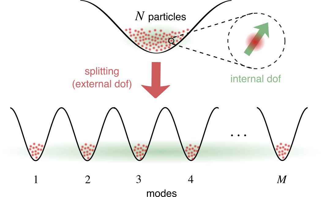
Figure 1: By spatially splitting an entangled ensemble of $N$ identical particles into $M$ external modes, we generate entanglement between addressable modes.

Particle entanglement can be revealed experimentally through spin-squeezing coefficients Wineland ; SorensenNature ; SorensenMolmer ; Ma ; GuehneToth ; Hyllus1 ; Hyllus2 . Among several methods to quantify spin squeezing Ma , the Wineland et al. spin-squeezing coefficient Wineland has the advantage of establishing a link between the entanglement detected in a quantum state and its quantum gain for interferometric measurements, thereby detecting metrologically useful entanglement PS09 . Moreover, this spin-squeezing coefficient expresses a sensitivity gain that can be reached by a simple parameter estimation protocol after sufficiently many experimental repetitions Wineland . Being a function of averages and variances of linear operators only, spin-squeezing coefficients are particularly suitable to detect multiparticle entanglement of spin states that can be approximated as Gaussian quantum states.

While particle entanglement can be detected with collective measurements, standard methods to reveal mode entanglement require local measurements on each mode. Criteria based on variances and mean values can be found in the form of modified uncertainty relations that hold for arbitrary separable states, but can be violated through entanglement DGCZ ; Raymer ; Giovannetti ; Werner ; HyllusEisert . These approaches are powerful tools to detect entanglement in arbitrary-dimensional systems with high flexibility. They allow us to study entanglement between specific partitions of a composite system, thereby providing precise microscopic information about which subsystems share quantum correlations GessnerQuantum ; QinNPJQI2019 . These criteria exist for both discrete and continuous variables, and they can be extended to study the stronger class of quantum correlations known as steering that is at the heart of the Einstein-Podolsky-Rosen (EPR) paradox Reid1989 ; ReidRMP .

In this work, we show that under conditions that hold for a wide range of systems, the uncertainty-type mode-entanglement criteria coincide with the Wineland et al. spin-squeezing coefficient, which detects particle entanglement and quantifies the metrological quantum gain. This allows us to establish a direct relation between the detected entanglement of particles and modes, as well as the sensitivity of spin states. While this does not replace the need for multimode entanglement witnesses, our results reveal the required level of spin squeezing for the generation of multimode entanglement by distributing the spins into addressable modes, e.g., by splitting a BEC into individually addressable ensembles. By linking these quantities to the spin-squeezing coefficient, we further relate mode entanglement and EPR steering to the quantum advantage in metrology measurements. Finally, we improve the best known bounds on the number of entangled particles that can be identified from the spin-squeezing coefficient without knowledge of the average polarization, and we clarify the connection to the spin-squeezing multipartite entanglement criterion by Sørensen and Mølmer SorensenMolmer .

II Mode vs particle entanglement

A collection of systems (labeled $1,...,\Xi$) is entangled if their quantum state cannot be written as

$$\rho=\sum_{\gamma}p_{\gamma}\rho_{\gamma}^{(1)}\otimes\cdots\otimes\rho_{\gamma}^{(\Xi)}\;,$$ (1)

where $\sum_{\gamma}p_{\gamma}=1$ is a probability distribution, and $\rho_{\gamma}^{(i)}$ are density matrices for system $i$. The local systems may refer either to the $\Xi=N$ particles or to the $\Xi=M$ modes that they occupy, giving rise to particle or mode entanglement, respectively. In practice, determining whether a given quantum state allows for a decomposition of the form of Eq. (1) is an extremely hard task. One therefore relies on entanglement witnesses or, more generally, necessary conditions that any separable state must satisfy GuehneToth ; HuberReview . A violation of these criteria then represents a witness for entanglement.

II.1 Uncertainty-based mode-entanglement criterion

Criteria based on first and second moments of linear observables are powerful tools to detect entanglement DGCZ ; Raymer ; Hofmann ; GuehneToth and steering Reid1989 ; ReidRMP in arbitrary-dimensional systems with high flexibility. An important class of these criteria take on the form of Heisenberg-Robertson-type uncertainty relations, with a modified lower bound on the variances that can be violated by entangled states. The most general formulation of these criteria for bipartite systems was given by Giovannetti et al. in Ref. Giovannetti , where it was furthermore shown that (nonlinear) product criteria are generally more powerful than (linear) sum criteria (see also HyllusEisert ; ReidRMP ). In the context of atomic spin ensembles it is convenient to express these criteria in terms of collective spin observables. For the case of $N$ spins distributed into $M=2$ modes, labeled as $A,B$, these take the form ${\bm{S}}^{A}=\sum_{i\in A}{\bm{s}}^{(i)}/2$, ${\bm{S}}^{B}=\sum_{i\in B}{\bm{s}}^{(i)}/2$, where ${\bm{s}}^{(i)}$ is the spin for particle $i$. The criterion expresses that all mode-separable states satisfy

$$\mathcal{G}^{2}:=\dfrac{4\,\text{Var}\left[S_{z}^{A}+S_{z}^{B}\right]\,\text{Var}\left[S_{y}^{A}-S_{y}^{B}\right]}{\left(|\langle S_{x}^{A}\rangle|+|\langle S_{x}^{B}\rangle|\right)^{2}}\geq 1\;.$$ (2)

The choice of observables (e.g. local spin components) can further be optimized to identify the most sensitive entanglement criterion for a given quantum state. These criteria can be generalized to study entanglement in specific multipartitions (with precise microscopic information about which subsystems share quantum correlations) GessnerQuantum as well as full inseparability VanLoock ; Toscano ; ReidTeh ; RiedTehSpin , i.e. the violation of these bounds in all possible partitions.

II.2 Spin squeezing particle-entanglement criterion

In the case of a large number of spins, it becomes challenging to address each particle individually. Nevertheless, particle entanglement among the individual spins can be detected from collective measurements of the spin components through spin-squeezing criteria. For all fully separable spin$-1/2$ states it holds that

$$\xi^{2}:=\dfrac{N\,\text{Var}\left[S_{z}\right]}{|\langle S_{x}\rangle|^{2}}\geq 1\;,$$ (3)

where $\xi^{2}$ is the Wineland et al. spin-squeezing coefficient Wineland . States with $\xi^{2}<1$ are characterized by a variance of the collective spin operator that is smaller than that of a coherent spin state, while at the same time being strongly polarized along the $S_{x}$ direction.

The spin-squeezing coefficient can be considered as a simple Gaussian approximation of the full metrological sensitivity that can be extracted from the quantum state PS09 ; RMP ; GessnerPRL2019 . For this reason, states with $\xi^{2}<1$ can achieve a quantum enhancement beyond the standard quantum limit in metrology measurements Wineland and the entanglement revealed by this condition is metrologically useful. This approach can be extended to fluctuating particle numbers Hyllus1 , multipartite entanglement HyllusToth ; GessnerPRA2017 , Bell nonlocality Frowis , and to analyze the multimode entanglement structure in addressable systems of arbitrary dimension GessnerQuantum ; QinNPJQI2019 .

III Equivalence of mode and particle entanglement: Two-mode case

In the following we prove that, if the state of the system is symmetric under the exchange of particle labels and of modes, the two criteria (2) and (3) are equivalent, namely that

$$\mathcal{G}^{2}=\xi^{2}\;.$$ (4)

To show this, imagine a system of $i=1,\dots,N$ particles with an internal (spin) and an external (mode) dof. We associate to each particle the operator $s_{\vec{u}}^{(i)}\Pi^{I,(i)}$, where $s_{\vec{u}}^{(i)}$ is the spin operator along direction $\vec{u}$, and $\Pi^{I,(i)}$ is the projection operator of the external dof onto one of the $M=2$ modes labeled as $I=1\equiv A$ and $I=2\equiv B$. Let us now assume the following properties valid for all $i,j=1,\dots,N$, and $I,J=1,\dots,M\geq 2$:

1. dof’s factorize: there are no correlations between the spin and the spatial dof, e.g. $\left\langle s_{\vec{u}}^{(i)}\Pi^{I,(i)}\right\rangle=\left\langle s_{\vec{u}}^{(i)}\right\rangle\left\langle\Pi^{I,(i)}\right\rangle$, $\left\langle s_{\vec{u}}^{(i)}\Pi^{I,(i)}s_{\vec{v}}^{(j)}\Pi^{J,(j)}\right\rangle=\left\langle s_{\vec{u}}^{(i)}s_{\vec{v}}^{(j)}\right\rangle\left\langle\Pi^{I,(i)}\Pi^{J,(j)}\right\rangle$;

2. particle symmetry: the state is invariant under permutations of the particle labels, e.g. $\left\langle s_{\vec{u}}^{(i)}\right\rangle=\left\langle s_{\vec{u}}^{(1)}\right\rangle$, $\left\langle s_{\vec{u}}^{(i)}s_{\vec{v}}^{(j)}\right\rangle=\left\langle s_{\vec{u}}^{(1)}s_{\vec{v}}^{(2)}\right\rangle$ and $\left\langle\Pi^{I,(i)}\right\rangle=\left\langle\Pi^{I,(1)}\right\rangle$, $\left\langle\Pi^{I,(i)}\Pi^{J,(j)}\right\rangle=\left\langle\Pi^{I,(1)}\Pi^{J,(2)}\right\rangle$, for $i\neq j$;

3. symmetric splitting: a) there is equal probability for a particle to be found in any of the modes, i.e. $\left\langle\Pi^{I,(i)}\right\rangle=1/M$, and b) these probabilities are independent, i.e. $\left\langle\Pi^{I,(i)}\Pi^{J,(j)}\right\rangle=\left\langle\Pi^{I,(i)}\right\rangle\left\langle\Pi^{J,(j)}\right\rangle$.

Let us mention that these assumptions are relevant for a number of experimental systems. For example, they apply to an ensemble of identical atoms distributed symmetrically in a set of external modes, as in Refs. FadelSplitBEC ; KunkelSplitBEC ; LangeSplitBEC .

Exploiting assumptions (i) and (ii), we can now compute expectation values of collective spin observables as

$$\left\langle S_{\vec{u}}^{I}\right\rangle =\sum_{i=1}^{N}\left\langle s_{\vec{u}}^{(i)}\Pi^{I,(i)}\right\rangle$$

$$=\left\langle\Pi^{I}\right\rangle N\left\langle s_{\vec{u}}\right\rangle$$ (5)

Note that here, and in the following, we use the shorthand notation $\left\langle s_{\vec{u}}^{(1)}\right\rangle=\left\langle s_{\vec{u}}\right\rangle$ and $\left\langle\Pi^{I,(1)}\right\rangle=\left\langle\Pi^{I}\right\rangle$.

Similarly, we obtain that correlators take the form (see Appendix A.1 for details)

$$\left\langle S_{\vec{u}}^{I}S_{\vec{v}}^{J}\right\rangle= \delta_{I,J}\left\langle\Pi^{I}\right\rangle N\left\langle s_{\vec{u}}^{(1)}s_{\vec{v}}^{(2)}\right\rangle+$$

$$+\left\langle\Pi^{I}\right\rangle\left\langle\Pi^{J}\right\rangle N(N-1)\left\langle s_{\vec{u}}^{(1)}s_{\vec{v}}^{(2)}\right\rangle\;.$$ (6)

To prove now the relation Eq. (4), we use Eqs. (5) and (6) to rewrite the variance appearing in Eq. (2) as (see the Appendix A.2 for a detailed derivation)

$$\,\text{Var}\left[S_{y}^{A}-S_{y}^{B}\right]=2\langle\Pi^{A}\rangle\dfrac{N}{4}=\dfrac{N}{4}\;\quad\text{using (iii)}.$$ (7)

For the other variance in Eq. (2) we can simply write

$$\,\text{Var}\left[S_{z}^{A}+S_{z}^{B}\right]=\,\text{Var}\left[S_{z}\right]\;.$$ (8)

The same holds also for the denominator, which can be written as

$$\left(|\langle S_{x}^{A}\rangle|+|\langle S_{x}^{B}\rangle|\right)^{2}=|\langle S_{x}\rangle|^{2}\;,$$ (9)

since symmetry implies that $\langle S_{x}^{A}\rangle$ and $\langle S_{x}^{B}\rangle$ have the same sign. It is now straightforward to combine the results of Eqs. (7), (8), and (9) to see that, under the assumptions introduced before, we obtain Eq. (4).

This result highlights a correspondence of the detected mode entanglement in two addressable modes and the detected particle entanglement in fully symmetric many-body quantum states. In the following we further generalize this criterion to an arbitrary number of modes $M$, and show how full multipartite inseparability can be detected with these methods.

IV Generalization to multipartite entanglement

When considering a collection of systems, entanglement can emerge in different partitions of the ensemble, i.e. across any separation of the ensemble into groups of systems. Let us denote one specific partition as $\Lambda=\{\mathcal{A}_{1},\dots,\mathcal{A}_{k}\}$, where the $\mathcal{A}$’s are non-overlapping groups of $1\leq|\mathcal{A}_{q}|\leq\Xi$ systems, such that $\sum_{q=1}^{k}|\mathcal{A}_{q}|=\Xi$. An $\Xi$-partite quantum state $\rho$ is called $\Lambda$-separable if it can be written as

$$\rho_{\Lambda-\mathrm{sep}}=\sum_{\gamma}p_{\gamma}\rho_{\gamma}^{(\mathcal{A}_{1})}\otimes\cdots\otimes\rho_{\gamma}^{(\mathcal{A}_{k})}\;,$$ (10)

where the $\rho_{\gamma}^{(\mathcal{A}_{q})}$ are quantum states of the subsystem $\mathcal{A}_{q}$. For an overview of different classes of entangled states in multipartite systems, we refer to Appendix B.

IV.1 Inseparability of $M$ modes

The entanglement criterion (2) can be generalized to yield a criterion for $\Lambda$-separable states of an $M$-mode system as follows GessnerQuantum : Any $\Lambda$-separable state must satisfy

$$\mathcal{G}_{\Lambda}^{M}(\vec{g},\vec{h})^{2}:=\dfrac{\,\text{Var}\left[\sum_{I=1}^{M}g_{I}S_{z}^{I}\right]\,\text{Var}\left[\sum_{I=1}^{M}h_{I}S_{y}^{I}\right]}{\mathcal{B}_{\Lambda}^{M}(\vec{g},\vec{h})^{2}}\geq 1\;,$$ (11)

where

$$\mathcal{B}_{\Lambda}^{M}(\vec{g},\vec{h}):=\frac{1}{2}\sum_{q=1}^{l}\left|\sum_{I\in\mathcal{A}_{q}}g_{I}h_{I}\langle S^{I}_{z}\rangle\right|\;.$$ (12)

This bound holds for arbitrary choices of the coefficient vectors $\vec{g}=(g_{1},\dots,g_{M})$ and $\vec{h}=(h_{1},\dots,h_{M})$, which can be optimized to obtain the strongest possible witness. A violation of Eq. (11) witnesses inseparability in the partition $\Lambda$.

We may further exclude separability in all partitions $\Lambda$ that contain at most $k$ subsystems by observing a violation of the single condition

$$\mathcal{G}_{k}^{M}(\vec{g},\vec{h}):=\max_{\Lambda:\>l\geq k}\mathcal{G}_{\Lambda}^{M}(\vec{g},\vec{h})\geq 1,$$ (13)

where the maximization runs over all partitions that consist of $l\geq k$ subsystems. A violation of the above bound with $k=M$, where each mode is treated as an individual subsystem, indicates that there is entanglement somewhere in the system without specifying how many subsystems are entangled. If the bound is violated for $k=2$, this means that we cannot identify even two separable groups, and we must thus consider the ensemble of all spins as a single entangled system. We remark here that this criterion analyzes each partition on a one-by-one basis, but it does not exclude arbitrary mixtures of separable models for different partitions, which is known as genuine multipartite entanglement ReidTeh ; HyllusEisert ; GuehneToth (see Appendix B for details).

It is evident that the computation of the bound (13) becomes very demanding since the number of possible partitions increases exponentially with $M$. Moreover, identifying a suitable choice for the $\{\vec{g},\vec{h}\}$ introduces additional complexity. A special case of Eq. (11) is obtained for the choice of $\{\vec{g},\vec{h}\}$ given by

$$g_{I}^{\ast}=1\;,\qquad h_{1}^{\ast}=1\;,\qquad h_{J}^{\ast}=-\frac{1}{M-1}\;,$$ (14)

for all $I=1,\dots,M$ and $J=2,\dots,M$. With this choice we note that $g_{1}^{\ast}h_{1}^{\ast}=1$, and $g_{I}^{\ast}h_{I}^{\ast}=-(M-1)^{-1}$ for $I>1$.

Since for the symmetric spin states considered here, the variances in Eq. (11) do not depend on the partition $\Lambda$, the maximization in Eq. (13) affects only the bound (12). We thus obtain that $\mathcal{G}_{k}^{M}(\vec{g},\vec{h})=\mathcal{G}_{\Lambda_{\min}}^{M}(\vec{g},\vec{h})$, where $\Lambda_{\min}$ is the partition that achieves the minimum

$$\beta^{M}_{k}(\vec{g},\vec{h})=\frac{|\langle S_{z}^{A}\rangle|}{2}\min_{\Lambda:l\geq k}\beta^{M}_{\Lambda}(\vec{g},\vec{h})\;,$$ (15)

and $\beta^{M}_{\Lambda}(\vec{g},\vec{h}):=\sum_{q=1}^{l}\left|\sum_{I\in\mathcal{A}_{q}}g_{I}h_{I}\right|$. In writing Eq. (15), we made use of the symmetry property (5) to limit the optimization procedure to the coefficients $\{\vec{g},\vec{h}\}$. Next, we observe that all contributions of terms from sets with $I>1$ will increase $\beta^{M}_{\Lambda}(\vec{g}^{*},\vec{h}^{*})$ whenever they appear in a partition $\Lambda$ that distinguishes them from mode $I=1$, whereas these terms will decrease $\beta^{M}_{\Lambda}(\vec{g}^{*},\vec{h}^{*})$ when in a partition $\Lambda$ that lumps them into the set $\mathcal{A}_{1}$ together with mode $1$. From this argument we also see that it is advantageous to pick a partition that splits the system in as few subsystems as possible. Since for a given $k$, at least $k$ subsystems must be formed, the optimal partition describes $k-1$ single-mode subsystems (with $I>1$) and places all other modes (including $I=1$) into a single subsystem. The minimum bound is thus given by

$$\beta^{M}_{\Lambda}(\vec{g}^{*},\vec{h}^{*}) =|g_{1}^{\ast}h_{1}^{\ast}\underbrace{+\dots+g_{M-(k-1)}^{\ast}h_{M-(k-1)}^{\ast}}_{M-k\;\text{terms}}|$$

$$\quad+\underbrace{|g_{M-(k-2)}^{\ast}h_{M-(k-2)}^{\ast}|+\cdots+|g_{M}^{\ast}h_{M}^{\ast}|}_{k-1\;\text{terms}}$$

$$=\dfrac{2(k-1)}{M-1}\;.$$ (16)

In summary, the minimum bound at the denominator of Eq. (11) takes the form

$$\mathcal{B}_{k}^{M}(\vec{g}^{\ast},\vec{h}^{\ast})=\dfrac{1}{2}\left(\dfrac{2(k-1)}{M-1}\right)\left|\left\langle S_{x}^{A}\right\rangle\right|\;.$$ (17)

The choice given in Eq. (14) gives for the variances

$$\,\text{Var}\left[\sum_{I=1}^{M}g_{I}S_{z}^{I}\right]=\,\text{Var}\left[S_{z}\right]\;,$$ (18)

and, using again Eqs. (5) and (6) with $\left\langle\Pi^{I}\right\rangle=1/M$, that

$$\,\text{Var}\left[\sum_{I=1}^{M}h_{I}S_{y}^{I}\right]=\dfrac{N}{4(M-1)}\;.$$ (19)

A detailed calculation is given in Appendix C.

Using the definition of $\xi^{2}$ (3), together with Eqs. (17), (18) and (19), we can express Eq. (11) as

$$\mathcal{G}_{k}^{M}(\vec{g}^{\ast},\vec{h}^{\ast})^{2} =\xi^{2}\dfrac{M^{2}(M-1)}{4(k-1)^{2}}\geq 1\;.$$ (20)

From this, we conclude that any state that is separable into $k$ subsystems or more must satisfy

$$\xi^{2}\geq\dfrac{4(k-1)^{2}}{M^{2}(M-1)}\;.$$ (21)

Therefore, observing $\xi^{2}<4(k-1)^{2}/(M^{2}(M-1))$ implies more than $k$ partite inseparability (see blue lines in Fig. 2). This is the main result of this section. It implies, e.g. that mode entanglement $(k=M)$ is observed among $M$ modes whenever $M<2(1+\sqrt{1-\xi^{2}})/\xi^{2}$ (black line in Fig. 2).

Since any state can be considered as a single indivisible system, the bound becomes trivial for $k=1$ and it can never be violated in this case. Generally, meaningful values for $k$ range from $2$ to $M$, and the smaller $k$ is, the more modes are recognized as entangled. If the bound is violated for $k=2$ this implies that there is no separable partition at all, and hence all $M$ modes must be entangled. For $M=2$, the criterion Eq. (20) reduces to Eq. (4), as expected.

We recall that our conclusions are based on specific entanglement witnesses, i.e. sufficient conditions for entanglement. Hence, these results only put a lower bound on the actual number of entangled modes.

IV.2 Limits on global and local spin-squeezing

Let us now investigate the lower bound for the spin-squeezing coefficient $\xi^{2}$. As we show in Appendix D.1, an arbitrary spin-$S$ system always satisfies the bound

$$\xi^{2}\geq\frac{1}{1+S}\;,$$ (22)

where the equality can be approached asymptotically.

Furthermore, we can define the local spin-squeezing coefficient

$$\xi^{2}_{I}:=\dfrac{N^{I}\,\text{Var}\left[S_{z}^{I}\right]}{|\langle S_{x}^{I}\rangle|^{2}}\;,$$ (23)

and show that there exists a limit on the squeezing that can be achieved locally from the splitting of a symmetric squeezed state. Under the assumptions (i), (ii) and (iiib) of Sec. III, the local squeezing obeys the bound

$$\xi^{2}_{I}\geq 1-\left\langle\Pi^{I}\right\rangle\;,$$ (24)

where the equality can be approached asymptotically in the limit $S\rightarrow\infty$ (see Appendix D.2). Let us emphasize that in the derivation of Eq. (24) we did not use assumption (iiia), meaning that the inequality holds even for asymmetric splittings into $M$ modes, i.e. for more general cases where $\left\langle\Pi^{I}\right\rangle$ depends on $I$.

To conclude, we can also show that there is an exact relation between the global and the local spin-squeezing coefficients, namely (see Appendix D.3)

$$\xi^{2}=\sum_{I=1}^{M}\xi^{2}_{I}-\dfrac{N^{2}(M-1)}{4\left\langle S_{x}\right\rangle^{2}}\;.$$ (25)

Also here, analogously to Eq. (24), it is worth emphasizing that Eq. (25) holds even for asymmetric splitting where $\left\langle\Pi^{I}\right\rangle$ depends on $I$. However, in the case where $\left\langle\Pi^{I}\right\rangle=1/M$, Eq. (25) can be used in conjunction with Eq. (21) to relate local squeezing and collective polarization to mode inseparability.

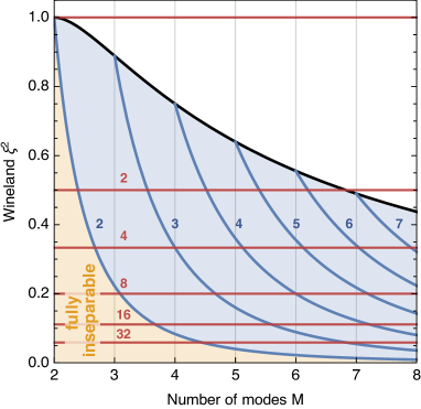
Figure 2: Bounds for mode and particle entanglement from collective spin measurements. We compare the Wineland et al. spin-squeezing coefficient to the limits on particle entanglement (28) (red lines) and mode entanglement for splitting into $M$ modes (21) (blue lines) as a function of $M$. For values of $\xi^{2}$ below the top black line (where $k=M$), mode entanglement is revealed. Upon crossing additional blue lines, the entanglement does not allow us to split the system into more than $k$ separable sets of modes, where $k$ is indicated in blue next to the lines. The yellow region corresponds to $k=2$, and it indicates where all modes must be treated as one entangled entity that cannot be partitioned into separable groups.

IV.3 Multipartite entanglement detection from spin squeezing

IV.3.1 State-independent multipartite entanglement bounds

Spin squeezing provides quantitative bounds on the number of entangled particles from collective measurements. Furthermore, the detected entanglement is relevant for the improvement of measurement precision in quantum metrology. To see this, recall that the quantum Fisher information $\mathcal{F}_{Q}[\rho,H]$ BraunsteinCaves quantifies the metrological sensitivity of a quantum state $\rho$ under an evolution generated by the Hamiltonian $H$ HelstromBook ; GiovannettiReview ; RMP . By virtue of the inequality PS09

$$\xi^{-2}\leq\frac{\mathcal{F}_{Q}[\rho,S_{y}]}{N},$$ (26)

the inverse spin-squeezing coefficient $\xi^{-2}$ can be interpreted as a Gaussian approximation to the full sensitivity, normalized by the total number of particles GessnerPRL2019 . The detection of metrologically useful entanglement makes use of the fact that $p$-producible $N$-qubit quantum states (i.e. states that contain at most $p$ entangled particles; see Appendix B) can only achieve sensitivites up to $\mathcal{F}_{Q}[\rho_{p},S_{y}]\leq pN$ PS09 ; HyllusToth . Combining this bound with the inequality (26), we find that a violation of GessnerPRA2017

$$\xi^{2}\geq\frac{1}{p}\;,$$ (27)

implies the presence of entanglement among more than $p$ particles (see blue lines in Fig. 3). For non-integer $N/p$ a small improvement of this bound can be achieved using a more general expression HyllusToth .

Interestingly, we can derive a much tighter bound than Eq. (27). This is possible because the limit $1/p$ arises from the bound on the quantum Fisher information that is achieved only by products of maximally entangled Greenberger-Horne-Zeilinger (GHZ) states HyllusToth , for which $\xi^{2}$ actually diverges, so that Eq. (27) can never be saturated. Instead, by making use of the asymptotically achievable limit (22), we can show that a violation of

$$\xi^{2}\geq\frac{1}{1+p/2}$$ (28)

implies entanglement of more than $p$ spins among the total number of $N$ spins-$1/2$ particles. This is the central result of this section and it follows as a consequence of convexity and subadditivity properties of the inverse spin-squeezing coefficient $\xi^{-2}$. The details can be found in Appendix E, where we also demonstrate that for non-integer $N/p$, the bound (28) can be improved to the expression:

$$\xi^{2}\geq\frac{N}{N_{p}\frac{p^{2}}{2}+\frac{r^{2}}{2}+N},$$ (29)

with $N_{p}=\lfloor N/p\rfloor$ and $r=N-pN_{p}$. We emphasize that, contrary to Eq. (27), this bound can be (asymptotically) saturated, and for $p$ large it is higher than Eq. (27) by a factor of two (see red solid lines in Fig. 3).

In a system with $p$ spin-$1/2$ particles, the bound (28) can be approached asymptotically in the limit of infinite squeezing and vanishing polarization $\left\langle S_{x}\right\rangle$. Such states are known as Twin-Fock states $|\Psi_{\rm TF}\rangle$ (see, e.g., Ref. Klempt for an experimental study of their metrological entanglement) and the bound (28) expresses their full sensitivity as quantified by the quantum Fisher information $\mathcal{F}_{Q}[|\Psi_{\rm TF}\rangle,S_{y}]=p(1+p/2)$ [compare Eqs. (28) and (26)]. By quantifying the maximum sensitivity achievable with Gaussian measurements, the result (28) implies that any sensitivity of $p$ spin-$1/2$ particles that exceeds this bound, i.e. any state with $\mathcal{F}_{Q}[\rho,S_{y}]>p(1+p/2)$, must necessarily be non-Gaussian in the sense that its metrological features cannot be captured through spin-squeezing coefficients.

IV.3.2 State-dependent multipartite entanglement bounds

In practice, in order to access $\xi^{2}$ one actually measures $\,\text{Var}[S_{z}]$ and $\left\langle S_{x}\right\rangle$ separately, rather than the ratio $\,\text{Var}[S_{z}]/\left\langle S_{x}\right\rangle^{2}$ itself. Having independent knowledge of these two quantities, it is possible to construct a stronger multipartite entanglement witness than Eq. (28). Sørensen and Mølmer SorensenMolmer showed that states with no more than $p$-partite entanglement satisfy

$$\,\text{Var}\left[S_{z}\right] \geq S\,F_{S_{p}}\left[\frac{\langle S_{x}\rangle}{S}\right],$$ (30)

where $S_{p}=p/2$, and the functions $F_{S}[x]$ are obtained (e.g. numerically) by minimizing the variance $\,\text{Var}[S_{z}]$ of a spin $S$ as a function of its mean spin $\left\langle S_{x}\right\rangle$ SorensenMolmer . This approach is constructed such that it detects the largest family of entangled states on the basis of $\,\text{Var}[S_{z}]$ and $\left\langle S_{x}\right\rangle$. However, since the metrological sensitivity is determined only by the ratio of these two quantities, the multipartite entanglement detected by this approach is not immediately linked to a metrological advantage. Yet, the criterion (30) is more powerful than Eq. (28), since it makes use of the additional information provided by $\left\langle S_{x}\right\rangle$. Indeed, we demonstrate in Appendix F.3 that in the limit $\left\langle S_{x}\right\rangle\to 0$, the condition (30) coincides with (28). Since this corresponds to the limit in which the criterion (30) is least effective, we can interpret this limit as ignoring the additional information that is provided by the mean spin length, assuming the worst-case scenario. This can be seen in Fig. 3, where we compare the constant bound for $p$-partite entanglement obtained from Eq. (28) (red continuous lines) to the state-dependent bound from Eq. (30) (red dashed lines).

We show in Appendix F.2 how condition (30) can be improved for non-integer $N/p$, and how the resulting expression reproduces the bound (29) in the limit of vanishing polarization $\left\langle S_{x}\right\rangle$. Condition (30) also allows to identify genuine $p$-partite entanglement ReidHeDrummundFrontiers2011 , meaning that one can exclude convex combinations of $(p-1)$-producible states (see Appendix B and F.4). Moreover, it can be generalized to systems with fluctuating particle numbers Hyllus2 .

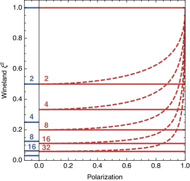
Figure 3: Detecting multiparticle entanglement from spin squeezing. A number $p$ of entangled particles is detected when the Wineland et al. spin-squeezing coefficient is lower than the respective lines. The solid blue lines are the constant bounds obtained from the Fisher information, Eq. (27). The solid red lines are improved bounds obtained from minimizing $\xi^{2}$ for fixed $S=p/2$, Eq. (28). These bounds are independent of the polarization $\left\langle S_{x}\right\rangle/S$. In contrast, the dashed lines are state-dependent bounds obtained from the Sørensen-Mølmer relation Eq. (30), where $\xi^{2}$ is minimized numerically for a fixed $S=p/2$ and polarization SorensenMolmer . The state-independent bounds (28) can be recovered from this approach in the limit of vanishing contrast.

V Relation with two-way EPR steering

For a bipartite scenario ($M=2$) the criterion Eq. (2) can be extended to detect also a stronger form of entanglement, namely EPR steering. Specifically, states that do not allow for steering of system $B$ by $A$ satisfy the condition CavalcantiReid ; Bowen ; ReidRMP

$$\mathcal{R}^{2}:=\dfrac{4\,\text{Var}\left[S_{z}^{A}+S_{z}^{B}\right]\,\text{Var}\left[S_{y}^{A}-S_{y}^{B}\right]}{|\langle S_{x}^{B}\rangle|^{2}}\geq 1\;.$$ (31)

Therefore, a violation of Eq. (31) reveals steering of $B$ by $A$. A similar criterion holds for steering of $A$ by $B$.

In the following we will focus on the symmetric scenario, where measurements in system $A$ and $B$ yield the same results. In this case we have $\left\langle S_{x}^{A}\right\rangle=\left\langle S_{x}^{B}\right\rangle$ which allows us to express the condition (31) equivalently as

$$\mathcal{R}^{2}=4\mathcal{G}^{2}=4\xi^{2}\geq 1\;.$$ (32)

Because of symmetry, a violation of this relation directly implies two-way steering between modes $A$ and $B$.

Combined with our results from the previous section, we conclude that if we want to observe steering through Eq. (31), we need to satisfy the condition $\xi^{2}<1/4$, which implies entanglement of $p>6$ particles. However, note that Eq. (31) can be generalized by including free coefficients in front of the spin operators, similarly to Eq. (11). This allows to detect EPR correlations with less squeezing FadelSplitBEC , but the correspondence given in Eq. (32) is lost.

Interestingly, a bipartite EPR criterion can also be derived from the Sørensen-Mølmer bounds Eq. (30). We show in Appendix F.5 that a violation of

$$\,\text{Var}[S_{z}]\geq S_{B}\,F_{S_{B}}\left[\dfrac{\langle S_{x}^{B}\rangle}{S_{B}}\right]$$ (33)

implies steering of $B$ by $A$. This criterion is easier to violate than the condition $\,\text{Var}[S_{z}]\geq S\,F_{S_{B}}\left[\dfrac{\langle S_{x}^{B}\rangle}{S}\right]$ that was derived in Ref. ReidHeDrummundFrontiers2011 . However, it is still very demanding to witness steering with this approach, since no assumptions can be made about the properties of system $A$.

VI Discussions and conclusions

In this work we established relations between criteria for multipartite entanglement of particles and modes based on the measurement of first and second moments of collective spin observables. In the case of symmetric spin states, we found that the Wineland et al. spin-squeezing coefficient Wineland coincides with a witness of mode entanglement that is based on Heisenberg-Robertson-type uncertainty relations with modified bounds Giovannetti . This correspondence can be extended to reveal a direct relation between the spin-squeezing coefficient of symmetric spin states and a two-way EPR-steering criterion of two addressable modes.

We further revealed the relation between different multipartite entanglement criteria based on spin squeezing. The Wineland et al. spin-squeezing coefficient Wineland captures the metrological sensitivity gain and can be used to study multiparticle entanglement. The approach by Sørensen and Mølmer SorensenMolmer makes use of the independent knowledge of the spin polarization to derive optimized state-dependent bounds on the spin-squeezing coefficient for multipartite entangled states. Alternatively, state-independent bounds can be derived by exploiting the relation between spin squeezing and the Fisher information PS09 , but these bounds are not saturable by Gaussian states HyllusToth . We addressed this limitation by deriving state-independent bounds that can be asymptotically saturated. This provides the tightest state-independent bounds on the spin-squeezing coefficient for the detection of multipartite entangled states. Interestingly, we observe that these bounds coincide with those of Sørensen and Mølmer SorensenMolmer in the limit of vanishing polarization.

Moreover, we identified a simple expression for the maximum spin squeezing that can be achieved locally from the splitting of a squeezed state. Our results provide bounds on the amount of addressable multimode entanglement that can be generated by distributing identical particles into external modes. For example, they apply to nonclassical states of BECs that are split into different spatial modes, as in Refs. FadelSplitBEC ; KunkelSplitBEC ; LangeSplitBEC .

VII Acknowledgments

We thank Qiongyi He, Margaret Reid, Run Yan Teh and Philipp Treutlein for useful discussions. MF acknowledges support by the Swiss National Science Foundation. MG acknowledges funding by the LabEx ENS-ICFP: ANR-10-LABX-0010/ANR-10-IDEX-0001-02 PSL*.

Supplementary material

Here we show the detailed calculations for the results presented in the paper.

Appendix A Detailed calculations for proving Eq. (4)

A.1 Proof of Eq. (6)

$$\left\langle S_{\vec{u}}^{I}S_{\vec{v}}^{J}\right\rangle =\sum_{i,j=1}^{N}\left\langle s_{\vec{u}}^{(i)}s_{\vec{v}}^{(j)}\Pi^{I,(i)}\Pi^{J,(j)}\right\rangle$$ (34a)

$$=\sum_{i=1}^{N}\left\langle s_{\vec{u}}^{(i)}s_{\vec{v}}^{(i)}\Pi^{I,(i)}\Pi^{J,(i)}\right\rangle+\sum_{\begin{subarray}{c}i,j=1\\ i\neq j\end{subarray}}^{N}\left\langle s_{\vec{u}}^{(i)}s_{\vec{v}}^{(j)}\Pi^{I,(i)}\Pi^{J,(j)}\right\rangle$$ (34b)

$$=\sum_{i=1}^{N}\left\langle s_{\vec{u}}^{(i)}s_{\vec{v}}^{(i)}\right\rangle\left\langle\Pi^{I,(i)}\Pi^{J,(i)}\right\rangle+\sum_{\begin{subarray}{c}i,j=1\\ i\neq j\end{subarray}}^{N}\left\langle s_{\vec{u}}^{(i)}s_{\vec{v}}^{(j)}\right\rangle\left\langle\Pi^{I,(i)}\Pi^{J,(j)}\right\rangle$$ using (i) (34c)

$$=\sum_{i=1}^{N}\left\langle s_{\vec{u}}^{(i)}s_{\vec{v}}^{(i)}\right\rangle\delta_{I,J}\left\langle\Pi^{I,(i)}\right\rangle+\sum_{\begin{subarray}{c}i,j=1\\ i\neq j\end{subarray}}^{N}\left\langle s_{\vec{u}}^{(i)}s_{\vec{v}}^{(j)}\right\rangle\left\langle\Pi^{I,(i)}\Pi^{J,(j)}\right\rangle$$ projectors are orthogonal (34d)

$$=\delta_{I,J}\left\langle\Pi^{I}\right\rangle\sum_{i=1}^{N}\left\langle s_{\vec{u}}^{(i)}s_{\vec{v}}^{(i)}\right\rangle+\left\langle\Pi^{I}\right\rangle\left\langle\Pi^{J}\right\rangle\sum_{\begin{subarray}{c}i,j=1\\ i\neq j\end{subarray}}^{N}\left\langle s_{\vec{u}}^{(i)}s_{\vec{v}}^{(j)}\right\rangle$$ using (ii, iiib) (34e)

$$=\delta_{I,J}\left\langle\Pi^{I}\right\rangle N\left\langle s_{\vec{u}}^{(1)}s_{\vec{v}}^{(1)}\right\rangle+\left\langle\Pi^{I}\right\rangle\left\langle\Pi^{J}\right\rangle N(N-1)\left\langle s_{\vec{u}}^{(1)}s_{\vec{v}}^{(2)}\right\rangle\;.$$ (34f)

Moreover, if $\vec{u}=\vec{v}$ we obtain

$$\left\langle S_{\vec{u}}^{I}S_{\vec{u}}^{J}\right\rangle=\delta_{I,J}\left\langle\Pi^{I}\right\rangle N\dfrac{1}{4}+\left\langle\Pi^{I}\right\rangle\left\langle\Pi^{J}\right\rangle N(N-1)\left\langle s_{\vec{u}}^{(1)}s_{\vec{u}}^{(2)}\right\rangle\;.$$ (35)

A.2 Proof of Eq. (7)

Let us first express the variance and covariance of collective spins under the assumptions of symmetry. We obtain

$$\,\text{Var}\left[S_{\vec{u}}^{A}\right] =\left\langle(S_{\vec{u}}^{A})^{2}\right\rangle-\left\langle S_{\vec{u}}^{A}\right\rangle^{2}$$

$$=\left(\left\langle\Pi^{A}\right\rangle N\dfrac{1}{4}+\left\langle\Pi^{A}\right\rangle^{2}N(N-1)\left\langle s_{\vec{u}}^{(1)}s_{\vec{v}}^{(2)}\right\rangle\right)-\left(\left\langle\Pi^{A}\right\rangle N\left\langle s_{\vec{u}}^{(1)}\right\rangle\right)^{2}$$ (36)

and

$$\,\text{Cov}\left[S_{\vec{u}}^{A},S_{\vec{u}}^{B}\right] =\left\langle S_{\vec{u}}^{A}S_{\vec{u}}^{B}\right\rangle-\left\langle S_{\vec{u}}^{A}\right\rangle\left\langle S_{\vec{u}}^{B}\right\rangle$$

$$=\left(\left\langle\Pi^{A}\right\rangle\left\langle\Pi^{B}\right\rangle N(N-1)\left\langle s_{\vec{u}}^{(1)}s_{\vec{v}}^{(2)}\right\rangle\right)-\left(\left\langle\Pi^{A}\right\rangle N\left\langle s_{\vec{u}}^{(1)}\right\rangle\right)\left(\left\langle\Pi^{B}\right\rangle N\left\langle s_{\vec{u}}^{(1)}\right\rangle\right)$$

$$=\left(\left\langle\Pi^{A}\right\rangle^{2}N(N-1)\left\langle s_{\vec{u}}^{(1)}s_{\vec{v}}^{(2)}\right\rangle\right)-\left(\left\langle\Pi^{A}\right\rangle N\left\langle s_{\vec{u}}^{(1)}\right\rangle\right)^{2}.$$ (37)

Combining these expressions, we obtain

$$\,\text{Var}\left[S_{y}^{A}-S_{y}^{B}\right] =\,\text{Var}\left[S_{y}^{A}\right]+\,\text{Var}\left[S_{y}^{B}\right]-2\,\text{Cov}\left[S_{y}^{A},S_{y}^{B}\right]$$

$$=2\langle\Pi^{A}\rangle\dfrac{N}{4}\;.$$ (38)

Appendix B Definitions of multipartite entanglement

We briefly review different inequivalent notions of entanglement in multipartite systems. The definition provided in Eq. (10) of the main text describes separability in a specific partition $\Lambda=\{\mathcal{A}_{1},\dots,\mathcal{A}_{l}\}$, where each of the $\mathcal{A}_{q}$ is a group of $|\mathcal{A}_{q}|$ systems. Such a partition $\Lambda$ can be characterized either by the size of its largest group $w(\Lambda):=\max_{q}|\mathcal{A}_{q}|$ or by the number of groups it contains $h(\Lambda):=l$ (these two quantities correspond to width $w$ and height $h$ of the Young diagram associated with $\Lambda$ SzalayQuantum ). Separable models with $w(\Lambda)\leq p$ are called $p$-producible and those with $h(\Lambda)\geq k$ are called $k$-separable. These definitions can be applied to classify the type of correlations in the context of particle entanglement, where each particle is considered as a system, and mode entanglement, where each mode is considered as a system.

In the context of this paper, we provide criteria for “$k$-inseparable” states of modes, i.e. states that are incompatible with all mode-separable models (10) with $h(\Lambda)\geq k$. In the above definition, all separable models are excluded individually, i.e. we verify incompatibility with all descriptions of the kind (10) for each $\Lambda$ in $\mathfrak{L}_{k-\mathrm{sep}}=\{\Lambda\>|\>h(\Lambda)\geq k\}$. A stronger condition requires the exclusion of all convex combinations of a specific family of separable models, and it is usually emphasized by the term “genuine”, see e.g. Ref. ReidTeh . For instance, we would call a state genuine $k$-inseparable if it is incompatible with any description of the kind

$$\rho=\sum_{\Lambda\in\mathfrak{L}_{k-\mathrm{sep}}}P_{\Lambda}\rho_{\Lambda-\rm{sep}},$$ (39)

where $P_{\Lambda}$ is a probability distribution and the $\rho_{\Lambda-\rm{sep}}$ are of the form (10). In the context of particle entanglement, we further say that a state has [genuine] $p$-partite entanglement if it excludes all [convex combinations of] $(p-1)$-producible models (recall that $p$-producible models are described by the set $\mathfrak{L}_{p-\mathrm{prod}}=\{\Lambda\>|\>w(\Lambda)\leq p\}$).

Appendix C Detailed calculations for proving Eq. (20)

C.1 Proof of Eq. (15)

For a given $k$, one has to find the minimum among the bounds given by each partition. However, we can easily see that, because of the signs, the minimum bound will come from terms of the form

$$\mathcal{B}(M,k)=|g_{1}^{\ast}h_{1}^{\ast}\underbrace{-g_{2}^{\ast}h_{2}^{\ast}-\cdots}_{M-k\;\text{terms}}|+\underbrace{|g_{I}^{\ast}h_{I}^{\ast}|+\cdots+|g_{M}^{\ast}h_{M}^{\ast}|}_{k-1\;\text{terms}}\;.$$ (40)

This is because $g_{1}^{\ast}h_{1}^{\ast}=1$ is the largest term, that can be minimized by subtracting as many terms $g_{I}^{\ast}h_{I}^{\ast}$ with $I>0$ as possible.

Our choices give, for $0\geq c,d\geq M-1$

$$|g_{1}^{\ast}h_{1}^{\ast}+c\;g_{2}^{\ast}h_{2}^{\ast}| =\dfrac{M-1-c}{M-1}$$ (41a)

$$|d\;g_{2}^{\ast}h_{2}^{\ast}| =\dfrac{d}{M-1}$$ (41b)

and, with $c=M-k$, $d=k-1$, we get $\beta_{k}^{M}$.

C.2 Proof of Eq. (19)

$$\,\text{Var}\left[\sum_{I=1}^{M}h_{I}S_{\vec{u}}^{I}\right] =\sum_{I,J=1}^{M}\,\text{Cov}\left[h_{I}S_{\vec{u}}^{I},h_{J}S_{\vec{u}}^{J}\right]$$

$$=\sum_{I=1}^{M}h_{I}^{2}\,\text{Var}\left[S_{\vec{u}}^{I}\right]+\sum_{I\neq J=1}^{M}h_{I}h_{J}\,\text{Cov}\left[S_{\vec{u}}^{I},S_{\vec{u}}^{J}\right]$$

$$=T_{1}\left(\sum_{I=1}^{M}h_{A}^{2}\right)+T_{2}\left(\sum_{I=1}^{M}h_{I}^{2}+\sum_{I\neq J=1}^{M}h_{I}h_{J}\right)$$ (42)

with

$$T_{1} =\left\langle\Pi^{I}\right\rangle\dfrac{N}{4}$$ (43)

$$T_{2} =\left\langle\Pi^{I}\right\rangle^{2}N(N-1)\left\langle s_{\vec{u}}^{(1)}s_{\vec{v}}^{(2)}\right\rangle-\left(\left\langle\Pi^{I}\right\rangle N\left\langle s_{\vec{u}}^{(1)}\right\rangle\right)^{2}\;.$$ (44)

With the choice $h_{1}^{\ast}=1$ and $h_{I}^{\ast}=(M-1)^{-1}$ for $I>1$, we have

$$\sum_{I=1}^{M}{h_{I}^{\ast}}^{2}=\dfrac{M}{M-1}\;,\qquad\sum_{I\neq J=1}^{M}h_{I}^{\ast}h_{J}^{\ast}=-\dfrac{M}{M-1}$$ (45)

and, therefore, taking $\left\langle\Pi^{I}\right\rangle=1/M$, we have

$$\,\text{Var}\left[\sum_{I=1}^{M}h_{I}^{\ast}S_{\vec{u}}^{I}\right]=\dfrac{N}{4(M-1)}\;,$$ (46)

a result that is independent of the state and of the direction $\vec{u}$.

Appendix D Limits on spin squeezing

D.1 Ultimate limit on spin squeezing

For a given, integer spin length $S$, we determine the minimum possible value of $\xi^{2}$ attainable by any quantum state. Our aim is to identify states with minimal $\,\text{Var}{[S_{z}]}$ with fixed $\left\langle S_{x}\right\rangle$. Sørensen and Mølmer SorensenMolmer pointed out that these states satisfy $\left\langle S_{z}\right\rangle=0$ and can therefore be found as the ground states of the Hamiltonian $H=\lambda S_{x}+S_{z}^{2}$, where $\lambda$ takes on the role of a Lagrange multiplier, see also RojoPRA2003 . We use first-order perturbation theory to determine the value of $\xi^{2}$ for the ground state in the presence of some small but finite $\lambda$, and then take the limit $\lambda\to 0$. We start from the ground state of the (unperturbed) Hamiltonian $H_{0}=S_{z}^{2}$, which is the state $|S,m_{z}\rangle=|S,0\rangle$. Considering $S_{x}$ as the perturbation, the ground state of $H$ to first order in $\lambda$ is (up to normalization)

$$|\tilde{\psi}\rangle =|S,0\rangle+\lambda\sum_{m\neq 0}\dfrac{\langle m,S|S_{x}|S,0\rangle}{E_{0}-E_{m}}|S,m\rangle$$ (47)

$$=|S,0\rangle-\lambda\dfrac{1}{2}\sqrt{S(S+1)}\left(|S,-1\rangle+|S,+1\rangle\right)\;,$$ (48)

where $E_{m}=\langle S,m|H_{0}|S,m\rangle$, and given the form of $S_{x}$ the summation effectively runs only over $m=\pm 1$. We use this expression (plus normalization) to evaluate the expectation values

$$\left\langle S_{x}\right\rangle =-\dfrac{2S(S+1)\lambda}{2+S(S+1)\lambda^{2}}$$ (49)

$$\left\langle S_{z}^{2}\right\rangle =1-\dfrac{2}{2+S(S+1)\lambda^{2}}\;.$$ (50)

The spin-squeezing coefficient obtained from these expressions reads

$$\xi^{2}=\dfrac{1}{S+1}+\dfrac{S}{2}\lambda^{2}\;.$$ (51)

We conclude that, in any spin-$S$ system, we have

$$\xi^{2}\geq\dfrac{1}{S+1}.$$ (52)

As explained in the main text, this limit corresponds to the sensitivity of a twin-Fock state $|S,0\rangle$ (as expressed by its quantum Fisher information).

D.2 Limit on local spin squeezing after splitting

Let us now identify the limit of the local spin-squeezing coefficient in one of the modes after splitting an ensemble described by the global coefficient $\xi^{2}$ into $M$ modes. We can define the local spin-squeezing coefficient as

$$\xi_{I}^{2}:=\dfrac{N^{I}\,\text{Var}\left[S_{z}^{I}\right]}{|\langle S_{x}^{I}\rangle|^{2}}\;,$$ (53)

where $N^{I}=N\left\langle\Pi^{I}\right\rangle$ and, using Eqs. (5) and (36), we find that the relation with the total squeezing $\xi^{2}$ is

$$\xi_{I}^{2}=\xi^{2}\left\langle\Pi^{I}\right\rangle+\left(1-\left\langle\Pi^{I}\right\rangle\right)\left(\dfrac{N\left\langle\Pi^{I}\right\rangle/2}{\left\langle S_{x}^{I}\right\rangle}\right)^{2}\;.$$ (54)

Because $\xi^{2}\geq 0$ and $N\left\langle\Pi^{I}\right\rangle/2\left\langle S_{x}^{I}\right\rangle\geq 1$, we obtain that

$$\xi_{I}^{2}\geq 1-\left\langle\Pi^{I}\right\rangle\;.$$ (55)

This expression tells us that, even if the intitial state comes close to the limit $\xi^{2}\rightarrow 0$ and $\left\langle S_{x}^{I}\right\rangle\rightarrow N\left\langle\Pi^{I}\right\rangle/2$ (which can be approached in the limit $N\rightarrow\infty$ with optimized squeezing), after the splitting the squeezing will always be limited by (55). If $\left\langle\Pi^{I}\right\rangle=1/2$, one obtains locally at most $-3\;\text{dB}$ of spin squeezing. If $\left\langle\Pi^{I}\right\rangle=1/3$, $\xi_{I}^{2}\geq-1.76\;\text{dB}$.

D.3 Relation between global and local squeezing

To relate the global squeezing $\xi^{2}$ to the sum of local squeezing coefficients $\xi^{2}_{I}$, we make use of Eq. (5) to rewrite Eq. (54) as:

$$\xi^{2}\left\langle\Pi^{I}\right\rangle=\xi_{I}^{2}-\left(1-\left\langle\Pi^{I}\right\rangle\right)\left(\dfrac{N}{2\left\langle S_{x}\right\rangle}\right)^{2}\;.$$ (56)

Summing both sides over all modes $I=1,\dots,M$, and using the fact that $\sum_{I=1}^{M}\left\langle\Pi^{I}\right\rangle=1$, we obtain Eq. (25).

Appendix E Derivation of sharper multipartite entanglement bounds on $\xi^{2}$

Our derivation of the criterion for $p$-partite entanglement (28) makes use of the ultimate limit on the spin-squeezing coefficient $\xi^{2}$ in arbitrary quantum states of a spin-$S$ system that was derived in Appendix D.1. We further use convexity and subadditivity of the inverse spin-squeezing coefficient, which we demonstrate below. Finally, we combine these results to derive the bound (28) on $p$-producible states.

E.1 Convexity and subadditivity of $(2S)\xi^{-2}$

Consider an arbitrary linear combination of quantum states $\rho=\sum_{\gamma}p_{\gamma}\rho_{\gamma}$. The inverse spin-squeezing coefficient satisfies the convexity property GessnerPRL2019

$$\xi^{-2}_{\rho}\leq\sum_{\gamma}p_{\gamma}\xi^{-2}_{\rho_{\gamma}}.$$ (57)

Let us demonstrate that $(2S)\xi^{-2}_{\rho}$ is also subadditive, where $S$ is the total spin of the system described by $\rho$. To this end, we consider a product state $\rho=\rho_{1}\otimes\cdots\otimes\rho_{M}$ and we decompose the total spin $S$ into its local components as $S_{\vec{u}}=\sum_{I=1}^{M}S_{\vec{u}}^{I}$. We write

$$(2S)\xi^{-2}_{\rho}=\frac{\left\langle S_{x}\right\rangle_{\rho}}{\,\text{Var}{[S_{z}]}_{\rho}},$$ (58)

and the absence of correlations in $\rho$ implies that

$$\left\langle S_{x}\right\rangle_{\rho} =\sum_{I=1}^{M}\left\langle S_{x}^{I}\right\rangle_{\rho_{I}}$$ (59a)

$$\,\text{Var}{[S_{z}]}_{\rho} =\sum_{I=1}^{M}\,\text{Var}{[S_{x}^{I}]}_{\rho_{I}}.$$ (59b)

The Cauchy-Schwarz inequality leads to

$$\left(\sum_{I=1}^{M}\left\langle S_{x}^{I}\right\rangle_{\rho_{I}}\right)^{2}\leq\sum_{I=1}^{M}\,\text{Var}{[S_{z}^{I}]}_{\rho_{I}}\sum_{I=1}^{M}\frac{\left\langle S_{x}^{I}\right\rangle_{\rho_{I}}^{2}}{\,\text{Var}{[S_{z}^{I}]}_{\rho_{I}}},$$ (60)

and we obtain the subadditivity

$$(2S)\xi^{-2}_{\rho_{1}\otimes\cdots\otimes\rho_{M}}\leq\sum_{I=1}^{M}(2S_{I})\xi^{-2}_{\rho_{I}}.$$ (61)

E.2 Limits on spin squeezing for $p$-producible states

Consider a separable state of the form $\rho=\sum_{\gamma}p_{\gamma}\rho_{\gamma}^{1}\otimes\cdots\otimes\rho_{\gamma}^{M}$, where the $\rho_{\gamma}^{I}$ are density matrices of spin $S_{I}$-subsystems with $\sum_{I=1}^{M}S_{I}=S$. We obtain

$$(2S)\xi^{-2}_{\rho} \leq\sum_{\gamma}p_{\gamma}(2S)\xi^{-2}_{\rho_{\gamma}^{1}\otimes\cdots\otimes\rho_{\gamma}^{M}}$$ using Eq. (69) (62a)

$$\leq\sum_{\gamma}p_{\gamma}\sum_{I=1}^{M}(2S_{I})\xi^{-2}_{\rho_{\gamma}^{I}}$$ using Eq. (61) (62b)

$$\leq\sum_{\gamma}p_{\gamma}\sum_{I=1}^{M}(2S_{I})(S_{I}+1)$$ using Eq. (52) (62c)

$$=2\sum_{I=1}^{M}S_{I}^{2}+2S$$ . (62d)

Now we assume that the state $\rho$ is a $p$-producible state of $N$ spin-$1/2$ particles ($S=N/2$), i.e. that each of its subsystems contains at most $p$ spin-$1/2$ particles. This sets the upper limit $S_{I}\leq p/2$ on the maximum spin length of each subsystem. Under this constraint, the function $\sum_{I=1}^{M}S_{I}^{2}$ is maximized by creating the largest possible number of $N_{p}=\lfloor N/p\rfloor$ groups of the maximal size $p$, and a single group of size $r=N-pN_{p}$ containing the remaining particles. This yields

$$\sum_{I=1}^{M}S_{I}^{2}\leq N_{p}\left(\frac{p}{2}\right)^{2}+\frac{1}{4}r^{2}.$$ (63)

Inserting this into Eq. (62d) leads to the following condition for arbitrary $p$-producible $N$-qubit states:

$$N\xi^{-2} \leq N_{p}\frac{p^{2}}{2}+\frac{r^{2}}{2}+N.$$ (64)

We may equivalently write this condition as

$$\xi^{2} \geq\frac{N}{N_{p}\frac{p^{2}}{2}+\frac{r^{2}}{2}+N}.$$ (65)

Note that, whenever $N/p$ is an integer, we have $N_{p}=N/p$, and thus $r=0$, and the bound simplifies to

$$\xi^{2} \geq\frac{1}{1+p/2}.$$ (66)

According to Eq. (52) this corresponds to the limit on spin squeezing for the largest entangled subsystem with spin $S=p/2$.

Appendix F Relation between the spin-squeezing entanglement witnesses of Wineland et al. Wineland and Sørensen-Mølmer SorensenMolmer

The Wineland et al. spin-squeezing coefficient Wineland expresses the ratio mean spin length and minimal variance in an orthogonal direction. This ratio has a clear metrological interpretation and, as we have discussed in Appendix E, it can be related to multiparticle entanglement. An alternative approach has been proposed by Sørensen and Mølmer SorensenMolmer , who use the combined information of mean spin length and minimal variance (beyond only their ratio) to derive limits on multiparticle entanglement.

Here, we demonstrate that the entanglement witness that is given by the Wineland et al. spin-squeezing coefficient can be recovered from the approach of Sørensen and Mølmer in the limit of vanishing mean spin length, which corresponds to the scenario where their criterion is least effective.

F.1 Properties of the functions $F_{S}[x]$

We first review and generalize the approach of Sørensen and Mølmer SorensenMolmer . We define $F_{S}$ as the minimum variance of $S_{z}$ divided by $S$ for a spin-$S$ system as a function of $\langle S_{x}\rangle$, i.e.

$$\dfrac{\,\text{Var}\left[S_{z}\right]}{S}\geq F_{S}\left[\dfrac{\langle S_{x}\rangle}{S}\right],$$ (67)

holds for all states and can be saturated. A graphical illustration of these bounds is given in Fig. (4) and in Ref. SorensenMolmer .

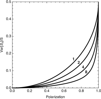
Figure 4: The Sørensen-Mølmer functions $F_{S}[x]$, Eq. (67), for different $S$ as a function of the polarization $x=\left\langle S_{x}\right\rangle/S$ SorensenMolmer .

Here $F_{S}[x]$ with $x\in[-1,1]$, is a function with the following properties (we assume $S$ integer, see Ref. SorensenMolmer for a discussion of non-integer cases):

• 0). $F_{S}[x]$ is symmetric in $x$, i.e. $F_{S}[-x]=F_{S}[x]$, with $F_{S}[0]=0$ and $F[\pm 1]=1/2$.

• 1). $F_{S}[x]$ is convex in $x$, i.e. $pF_{S}[x_{1}]+(1-p)F_{S}[x_{2}]\geq F_{S}[px_{1}+(1-p)x_{2}]$ for $0\leq p\leq 1$.

• 2). For $x\in[0,1]$, $F_{S}[x]$ is strictly increasing, i.e. for $x_{1}<x_{2}$, we have $F_{S}[x_{1}]<F_{S}[x_{2}]$.

• 3). For $S_{1}<S_{2}$ we have $F_{S_{1}}[x]>F_{S_{2}}[x]$.

• 4). The $F_{S}[x]$ satisfy $\lim_{x\rightarrow 0}\dfrac{F_{S}[x]}{x^{2}}=\dfrac{1}{2+2S}+O(x^{2})$.

• 5). For $x\geq 0$ and $\lambda>1$ it holds $F_{S}[\lambda x]\geq\lambda F_{S}[x]$.

The symmetry of property 0) follows directly from the definition Eq. (67), where the $x$-axis can always be chosen such that $\langle S_{x}\rangle\geq 0$. The value at $x=0$ follows from property 4), while the value at $x=1$ is attained by a spin-coherent state, with variance $\,\text{Var}[S_{z}]=S/2$. Properties 1) and 2) are proven in Ref. SorensenMolmer . Property 3) can be proven for large $S$ using the analytical expression SorensenMolmer

$$F_{S}[x]=\dfrac{1}{2}\left(1+S(1-x^{2})-\sqrt{(1-x^{2})((1+S)^{2}-S^{2}x^{2})}\right)\;,$$ (68)

valid for $S\gg 1$, while for smaller $S$, property 3) is confirmed numerically. Property 4) can be proven using the results Eqs. (49,50) obtained from perturbation theory (note that the limit $x=\left\langle S_{x}\right\rangle/S\rightarrow 0$ corresponds to the limit $\lambda\rightarrow 0$). In this case, $\xi^{2}/2\geq F_{S}[x]/x^{2}$, with equality when Eq. (67) is saturated and we obtain from Eq. (52) the desired limit. Note that if we were to take the limit using the expression Eq. (68), we would have obtained $1/(4+4S)$. The factor two difference is attributed to the fact that Eq. (68) is an approximation that differs from the true bound by a factor two in the limit of small $x$, as mentioned in Ref. SorensenMolmer . Finally, to prove property 5) we first use that the convexity of $F_{S}[x]$ is equivalent to the condition

$$F_{S}[x]\geq F^{\prime}_{S}[x_{0}](x-x_{0})+F_{S}[x_{0}]$$ (69)

for all $x,x_{0}\in[0,1]$. Using $F_{S}[0]=0$, we obtain at $x=0$

$$F^{\prime}_{S}[x_{0}]x_{0}\geq F_{S}[x_{0}].$$ (70)

At $x=\lambda x_{0}$ with $\lambda>1$, we can rewrite (69) as

$$F_{S}[\lambda x_{0}] \geq F^{\prime}_{S}[x_{0}](\lambda-1)x_{0}+F_{S}[x_{0}]$$

$$=(\lambda-1)(F^{\prime}_{S}[x_{0}]x_{0}-F_{S}[x_{0}])+\lambda F_{S}[x_{0}]$$

$$\geq\lambda F_{S}[x_{0}],$$ (71)

where in the last step, we used (70).

F.2 Generalization of the Sørensen-Mølmer bound to non-integer $N/p$

Sørensen and Mølmer proved their criterion for a decomposition of the total spin $S$ into $N/p$ subgroups of size $p$, assuming that $N/p$ is integer. Here, we generalize their result by considering a separation of the total system into as many groups as possible of maximal size $p$ plus a remaining group. More precisely, call $N_{p}=\lfloor N/p\rfloor$ the number of partitions into groups of $p$ particles. Each group has spin $S_{p}=p/2$ (for spin-$1/2$ particles). If $N/p$ is not an integer, there will be an additional group of $r=N-pN_{p}$ particles, labeled $r$(est), with spin $S_{r}=r/2$. We obtain

$$\,\text{Var}\left[S_{z}\right] \geq\sum_{\gamma}p_{\gamma}\left(\sum_{i=1}^{N_{p}}\,\text{Var}\left[S_{z}^{(i)}\right]_{\gamma}+\,\text{Var}\left[S_{z}^{(r)}\right]_{\gamma}\right)$$ concavity of the variance

$$\geq\sum_{\gamma}p_{\gamma}\left(\sum_{i=1}^{N_{p}}S_{p}\,F_{S_{p}}\left[\dfrac{\langle S_{x}^{(i)}\rangle_{\gamma}}{S_{p}}\right]+S_{r}\,F_{S_{r}}\left[\dfrac{\langle S_{x}^{(r)}\rangle_{\gamma}}{S_{r}}\right]\right)$$ using Eq. (67)

$$\geq\sum_{\gamma}p_{\gamma}\left((S_{p}N_{p})\,F_{S_{p}}\left[\dfrac{1}{S_{p}N_{p}}\sum_{i=1}^{N_{p}}\langle S_{x}^{(i)}\rangle_{\gamma}\right]+S_{r}\,F_{S_{r}}\left[\dfrac{\langle S_{x}^{(r)}\rangle_{\gamma}}{S_{r}}\right]\right)$$ using property 1)

$$\geq(S_{p}N_{p})\,F_{S_{p}}\left[\dfrac{1}{S_{p}N_{p}}\sum_{i=1}^{N_{p}}\sum_{\gamma}p_{\gamma}\langle S_{x}^{(i)}\rangle_{\gamma}\right]+S_{r}\,F_{S_{r}}\left[\sum_{\gamma}p_{\gamma}\dfrac{\langle S_{x}^{(r)}\rangle_{\gamma}}{S_{r}}\right]$$ using property 1)

$$=(S_{p}N_{p})\,F_{S_{p}}\left[\dfrac{1}{S_{p}N_{p}}\sum_{i=1}^{N_{p}}\langle S_{x}^{(i)}\rangle\right]+S_{r}\,F_{S_{r}}\left[\dfrac{\langle S_{x}^{(r)}\rangle}{S_{r}}\right].$$ (72)

This bound is the tightest formulation of the multipartite entanglement criterion first proposed by Sørensen and Mølmer in Ref. SorensenMolmer . It can be further simplified under the assumption of symmetric spin states. If property (ii) (see Sec. III in the main text) is granted, we may write $\langle S_{x}^{(i)}\rangle=p\langle S_{x}\rangle/N$ and $\langle S_{x}^{(r)}\rangle=r\langle S_{x}\rangle/N$. This yields

$$\,\text{Var}\left[S_{z}\right] \geq(S_{p}N_{p})\,F_{S_{p}}\left[\dfrac{1}{S_{p}N_{p}}N_{p}\frac{p}{N}\langle S_{x}\rangle\right]+S_{r}\,F_{S_{r}}\left[\frac{1}{S_{r}}\dfrac{r}{N}\langle S_{x}\rangle\right]$$

$$=(S_{p}N_{p})\,F_{S_{p}}\left[\frac{\langle S_{x}\rangle}{S}\right]+S_{r}\,F_{S_{r}}\left[\frac{\langle S_{x}\rangle}{S}\right],$$ (73)

where $S=N/2$ is the total spin.

By explicitly considering a subgroup of size $r$ when the distribution of $N$ particles into subgroups of size $p$ cannot account for all particles, this bound is stronger than the well-known bounds derived in SorensenMolmer . To see this, notice that $S_{r}<S_{p}$ and by virtue of property 3) we can thus derive the weaker bound

$$\,\text{Var}\left[S_{z}\right] \geq(S_{p}N_{p})\,F_{S_{p}}\left[\frac{\langle S_{x}\rangle}{S}\right]+S_{r}\,F_{S_{p}}\left[\frac{\langle S_{x}\rangle}{S}\right]$$

$$=S\,F_{S_{p}}\left[\frac{\langle S_{x}\rangle}{S}\right],$$ (74)

with $S=S_{p}N_{p}+S_{r}$. This is the standard formulation of the Sørensen-Mølmer multiparticle entanglement criterion SorensenMolmer and we observe that the condition (73) is indeed stronger. If $N_{p}$ is an integer, both criteria coincide, since $S_{r}=0$ and $S_{p}N_{p}=S$.

F.3 Relation between different spin-squeezing multiparticle entanglement criteria

Since the functions $F_{S}[x]$ are strictly increasing, the entanglement criterion (30) detects the largest number of entangled states when $\left\langle S_{x}\right\rangle$ is large. If, however, the value of $\left\langle S_{x}\right\rangle$ is not known separately from $\,\text{Var}{[S_{z}]}/\left\langle S_{x}\right\rangle^{2}$, we must assume the ‘worst-case scenario’, which consequently is given in the limit of $\left\langle S_{x}\right\rangle\rightarrow 0$. Here, we show that in this limit, the Sørensen-Mølmer approach to witnessing entanglement becomes equivalent to the bound (28) on the Wineland et al. spin-squeezing coefficient. We first demonstrate this correspondence for the simple bounds, i.e. Eqs. (28) and (30) and then generalize our result to the tighter expressions (65) and (72).

Note that the condition (30) for states with at most $p$-partite entanglement can be equivalently stated as

$$\frac{N\,\text{Var}\left[S_{z}\right]}{\left\langle S_{x}\right\rangle^{2}} \geq 2\,\frac{F_{S_{p}}\left[\frac{\langle S_{x}\rangle}{S}\right]}{\left(\frac{\left\langle S_{x}\right\rangle}{S}\right)^{2}}.$$ (75)

Making use of properties 2 and 4, we further obtain that

$$2\,\frac{F_{S_{p}}\left[\frac{\langle S_{x}\rangle}{S}\right]}{\left(\frac{\left\langle S_{x}\right\rangle}{S}\right)^{2}} \geq\frac{1}{\frac{p}{2}+1}.$$ (76)

Combining these two bounds, we can derive the multiparticle spin squeezing condition (28) in the ‘worst-case’ limit of the approach of Eq. (30).

Let us now demonstrate that the same correspondence holds for the most general formulation of the respective criteria for non-integer $N/p$. Using properties 2 and 4 in Eq. (72) implies that in the limits $\langle S_{x}^{(i)}\rangle\to 0$ and $\langle S_{x}^{(r)}\rangle\to 0$ the following condition holds for states with no more than $p$-partite entanglement:

$$\,\text{Var}\left[S_{z}\right] \geq\frac{\left(\sum_{i=1}^{N_{p}}\langle S_{x}^{(i)}\rangle\right)^{2}}{N_{p}\frac{p^{2}}{2}+pN_{p}}+\frac{\langle S_{x}^{(r)}\rangle^{2}}{\frac{r^{2}}{2}+r}.$$ (77)

We now demonstrate that the following statement holds for arbitrary $A,B,a,b\in\mathbb{R}$ with $a,b>0$:

$$\frac{A^{2}}{a}+\frac{B^{2}}{b}\geq\frac{(A+B)^{2}}{a+b}.$$ (78)

This relation follows immediately from

$$0\leq\frac{(Ab-aB)^{2}}{ab(a+b)}=\frac{A^{2}}{a}+\frac{B^{2}}{b}-\frac{(A+B)^{2}}{a+b}.$$ (79)

Using Eq. (78) with $A=\sum_{i=1}^{N_{p}}\langle S_{x}^{(i)}\rangle$, $B=\langle S_{x}^{(r)}\rangle$, $a=N_{p}\frac{p^{2}}{2}+pN_{p}$, and $b=\frac{r^{2}}{2}+r$, we obtain from Eq. (77) that

$$\,\text{Var}\left[S_{z}\right] \geq\frac{\left\langle S_{x}\right\rangle^{2}}{N_{p}\frac{p^{2}}{2}+\frac{r^{2}}{2}+N},$$ (80)

where we have used that $A+B=\sum_{i=1}^{N_{p}}\langle S_{x}^{(i)}\rangle+\langle S_{x}^{(r)}\rangle=\left\langle S_{x}\right\rangle$ and $pN_{p}+r=N$. Multiplying both sides of (80) by $N$ and dividing by $\left\langle S_{x}\right\rangle^{2}$, we recover the condition (65). This generalizes the correspondence between the two approaches to the stronger conditions, valid in the case of non-integer $N/p$.

F.4 Detecting genuine $p$-partite entanglement

Detecting genuine $(p+1)$-partite entanglement (recall Appendix B) requires to exclude not only each $p$-producible model individually but also all convex combinations of the kind

$$\rho=\sum_{\Lambda\in\mathfrak{L}_{p-\mathrm{prod}}}P_{\Lambda}\rho_{\Lambda-\mathrm{sep}}\;,$$ (81)

where each of the $\rho_{\Lambda-\rm{sep}}$ is of the form of Eq. (10). From the convexity of the spin-squeezing coefficient $\xi^{-2}_{\rho}$ [see Eq. (69)] we can immediately conclude that the bounds for $p$-producible states [see, e.g. Eq. (29)] also hold for arbitrary linear combinations of $p$-producible states, since the bounds are state independent.

This is not the case for the tighter bounds proposed by Sørensen and Mølmer, Eq. (30): These depend on the polarization which could be in principle different in each of the states $\rho_{\Lambda-\mathrm{sep}}$. The convexity property of the functions $F_{S}$ nevertheless allows us to interpret Eq. (30) as a criterion for genuine multipartite entanglement ReidHeDrummundFrontiers2011 .

We first establish the following property: Assume $S_{2}>S_{1}$, from the properties of the $F_{S}$ function we can write

$$S_{1}F_{S_{1}}[x_{1}]+S_{2}F_{S_{2}}[x_{2}] \geq S_{1}F_{S_{2}}[x_{1}]+S_{2}F_{S_{2}}[x_{2}]$$ using 3) (82a)

$$=(S_{1}+S_{2})\left(\dfrac{S_{1}}{S_{1}+S_{2}}F_{S_{2}}[x_{1}]+\dfrac{S_{2}}{S_{1}+S_{2}}F_{S_{2}}[x_{2}]\right)$$ (82b)

$$\geq(S_{1}+S_{2})F_{S_{2}}\left[\dfrac{S_{1}x_{1}+S_{2}x_{2}}{S_{1}+S_{2}}\right]\;.$$ using 1) (82c)

Consider the state Eq. (81) that is a convex combination of arbitrary $p$-producible models. Recall that each decomposition of the form of Eq. (10) depends on $\Lambda$, even though we do not make this dependence explicit below to simplify our notation. We further denote the total spin of subsystem $\mathcal{A}_{q}$ as $S_{q}=|\mathcal{A}_{q}|/2$. Using the concavity of the variance, we obtain

$$\,\text{Var}\left[S_{z}\right] \geq\sum_{\Lambda}\sum_{\gamma}P_{\Lambda}p_{\gamma}\left(\sum_{q=1}^{k}\,\text{Var}\left[S_{z}^{(k)}\right]_{\gamma}\right)$$

$$\geq\sum_{\Lambda}\sum_{\gamma}P_{\Lambda}p_{\gamma}\left(\sum_{q=1}^{k}S_{q}\,F_{S_{q}}\left[\dfrac{\langle S_{x}^{(q)}\rangle_{\gamma}}{S_{q}}\right]\right)\;.$$ (83)

Noticing that the largest possible value of all the $S_{q}$ is determined by $S_{p}=p/2$, we can apply property (82) successively to bound the sum over $q$, which gives

$$\,\text{Var}\left[S_{z}\right] \geq\sum_{\Lambda}\sum_{\gamma}P_{\Lambda}p_{\gamma}S\,F_{S_{p}}\left[\dfrac{\langle S_{x}\rangle_{\gamma}}{S}\right]\;,$$ (84)

where $S=\sum_{q=1}^{k}S_{q}$ and $\langle S_{x}\rangle_{\gamma}=\sum_{q=1}^{k}\langle S_{x}^{(q)}\rangle_{\gamma}$. Finally, using convexity of the $F_{S}$ functions [property 1)], we obtain the bound

$$\,\text{Var}\left[S_{z}\right] \geq S\,F_{S_{p}}\left[\sum_{\Lambda}\sum_{\gamma}P_{\Lambda}p_{\gamma}\dfrac{\langle S_{x}\rangle_{\gamma}}{S}\right]$$

$$=S\,F_{S_{p}}\left[\dfrac{\langle S_{x}\rangle}{S}\right]\;.$$ (85)

Therefore, finding the maximum integer $p$ for which this inequality is violated allows us to conclude that the state of the system is genuine $(p+1)$-partite entangled.

F.5 EPR steering criterion based on the Sørensen-Mølmer bounds Eq. (30)

Consider a fixed bi-partition of the system into $N_{A}$, $N_{B}=N-N_{A}$ particles. Steering of party $B$ by $A$ can be detected from the following criterion based on the Sørensen-Mølmer bounds Eq. (30). We first use the concavity of the variance to obtain

$$\,\text{Var}\left[S_{z}\right] \geq\sum_{\gamma}p_{\gamma}\left(\,\text{Var}\left[S_{z}^{A}\right]_{\gamma}+\,\text{Var}\left[S_{z}^{B}\right]_{\gamma}\right)$$ (86a)

$$\geq\sum_{\gamma}p_{\gamma}\,\text{Var}\left[S_{z}^{B}\right]_{\gamma}$$ (86b)

$$\geq\sum_{\gamma}p_{\gamma}S_{B}\,F_{S_{B}}\left[\dfrac{\langle S_{x}^{B}\rangle_{\gamma}}{S_{B}}\right]$$ (86c)

$$\geq S_{B}\,F_{S_{B}}\left[\sum_{\gamma}p_{\gamma}\dfrac{\langle S_{x}^{B}\rangle_{\gamma}}{S_{B}}\right]$$ (86d)

$$=S_{B}\,F_{S_{B}}\left[\dfrac{\langle S_{x}^{B}\rangle}{S_{B}}\right]\;.$$ (86e)

In the second step, we used the fact that in absence of a local quantum description of system $A$, we can only assume that $\,\text{Var}[S_{z}^{A}]\geq 0$, and the following steps follow from the properties of the $F_{S}$ functions.

In Ref. ReidHeDrummundFrontiers2011 , it was shown that steering is detected by a violation of the bound

$$\,\text{Var}\left[S_{z}\right]\geq S\,F_{S_{B}}\left[\frac{\langle S_{x}^{B}\rangle}{S}\right].$$ (87)

We now show that our condition (86a) implies Eq. (87) and is therefore a stronger steering witness. To see this, we denote $\lambda=S/S_{B}>1$ and write $S_{B}\,F_{S_{B}}[\dfrac{\langle S_{x}^{B}\rangle}{S_{B}}]=(S/\lambda)F_{S_{B}}[\lambda\dfrac{\langle S_{x}^{B}\rangle}{S}]\geq SF_{S_{B}}[\dfrac{\langle S_{x}^{B}\rangle}{S}]$, where in the last step we used the superlinear scaling of the $F_{S}[x]$, property 5) in Appendix F.1.

References

- (1) R. Horodecki, P. Horodecki, M. Horodecki, and K. Horodecki, Quantum entanglement, Rev. Mod. Phys. 81, 865 (2009).
- (2) J. J. Bollinger, W. M. Itano, D. J. Wineland, and D. J. Heinzen, Optimal frequency measurements with maximally correlated states, Phys. Rev. A 54, R4649 (1996).
- (3) L. Pezzè and A. Smerzi, Entanglement, Nonlinear Dynamics, and the Heisenberg Limit, Phys. Rev. Lett. 102, 100401 (2009).
- (4) P. Hyllus, W. Laskowski, R. Krischek, C. Schwemmer, W. Wieczorek, H. Weinfurter, L. Pezzé, and A. Smerzi, Fisher information and multiparticle entanglement, Phys. Rev. A 85, 022321 (2012); G. Tóth, Multipartite entanglement and high-precision metrology, Phys. Rev. A 85, 022322 (2012).
- (5) L. Pezzè, A. Smerzi, M. K. Oberthaler, R. Schmied, and P. Treutlein, Quantum metrology with nonclassical states of atomic ensembles, Rev. Mod. Phys. 90, 035005 (2018).
- (6) W. S. Bakr, J. I. Gillen, A. Peng, S. Fölling, and M. Greiner, A quantum gas microscope for detecting single atoms in a Hubbard-regime optical lattice, Nature 462, 74 (2009).
- (7) H. Labuhn, D. Barredo, S. Ravets, S. de Léséleuc, T. Macrì, T. Lahaye, and A. Browaeys, Tunable two-dimensional arrays of single Rydberg atoms for realizing quantum Ising models, Nature 534, 667 (2016).
- (8) A. Omran, H. Levine, A. Keesling, G. Semeghini, T. T. Wang, S. Ebadi, H. Bernien, A. S. Zibrov, H. Pichler, S. Choi, J. Cui, M. Rossignolo, P. Rembold, S. Montangero, T. Calarco, M. Endres, M. Greiner, V. Vuletić, M. D. Lukin, Generation and manipulation of Schrödinger cat states in Rydberg atom arrays, Science 365, 570 (2019).
- (9) M. Fadel, T. Zibold, B. Décamps and P. Treutlein, Spatial entanglement patterns and Einstein-Podolsky-Rosen steering in Bose-Einstein condensates, Science 360, 409 (2018).
- (10) P. Kunkel, M. Prüfer, H. Strobel, D. Linnemann, A. Frölian, T. Gasenzer, M. Gärttner and M. K. Oberthaler, Spatially distributed multipartite entanglement enables EPR steering of atomic clouds, Science 360, 413 (2018).
- (11) K. Lange, J. Peise, B. Lücke, I. Kruse, G. Vitagliano, I. Apellaniz, M. Kleinmann, G. Tóth and C. Klempt, Entanglement between two spatially separated atomic modes, Science 360, 416 (2018).
- (12) E. Oudot, J. D. Bancal, R. Schmied, P. Treutlein, and N. Sangouard, Optimal entanglement witnesses in a split spin-squeezed Bose-Einstein condensate, Phys. Rev. A 95, 052347 (2017).
- (13) Y. Jing, M. Fadel, V. Ivannikov, and T. Byrnes, Split spin-squeezed Bose–Einstein condensates, New J. Phys. 21, 093038 (2019).
- (14) P. C. Humphreys, M. Barbieri, A. Datta, and I. A. Walmsley, Quantum Enhanced Multiple Phase Estimation, Phys. Rev. Lett. 111, 070403 (2013)
- (15) T. J. Proctor, P. A. Knott, and J. A. Dunningham, Multiparameter Estimation in Networked Quantum Sensors, Phys. Rev. Lett. 120, 080501 (2018).
- (16) W. Ge, K. Jacobs, Z. Eldredge, A. V. Gorshkov, and M. Foss-Feig, Distributed Quantum Metrology and the Entangling Power of Linear Networks, Phys. Rev. Lett. 121, 043604 (2018).
- (17) M. Gessner, L. Pezzè, and A. Smerzi, Sensitivity Bounds for Multiparameter Quantum Metrology, Phys. Rev. Lett. 121, 130503 (2018).
- (18) D. Kajtoch, E. Witkowska and A. Sinatra, Spin-squeezed atomic crystal, Europhysics Letters 123, 20012 (2018).
- (19) M. Nielsen and I. Chuang, Quantum Computation and Quantum Information, (Cambridge University Press, Cambridge, 2000).
- (20) N. Killoran, M. Cramer and M. Plenio, Extracting Entanglement from Identical Particles, Phys. Rev. Lett. 112, 150501 (2014).
- (21) R. Lo Franco and G. Compagno, Indistinguishability of Elementary Systems as a Resource for Quantum Information Processing, Phys. Rev. Lett. 120, 240403 (2018).
- (22) B. Morris, B. Yadin, M. Fadel, T. Zibold, P. Treutlein and G. Adesso, Entanglement between identical particles is a useful and consistent resource,arXiv:1908.11735 (2019)
- (23) M. R. Barros, S. Chin, T. Pramanik, H.-T. Lim, Y.-W. Cho, J. Huh and Y.-S. Kim, Entangling Bosons through Particle Indistinguishability and Spatial Overlap, arXiv:1912.04208 (2019)
- (24) K. Sun, Y. Wang, Z.-H. Liu, X.-Y. Xu, J.-S. Xu, C.-F. Li, G.-C. Guo, A. Castellini, F. Nosrati, G. Compagno and R. Lo Franco, Experimental control of remote spatial indistinguishability of photons to realize entanglement and teleportation, arXiv:2003.10659 (2020).
- (25) O. Gühne and G. Tóth, Entanglement detection, Phys. Rep. 474, 1 (2009).
- (26) J. Ma, X. Wang, C. Sun, and F. Nori, Quantum spin squeezing, Phys. Rep. 509, 89 (2011).
- (27) D. J. Wineland, J. J. Bollinger, W. M. Itano, F. L. Moore, and D. J. Heinzen, Spin squeezing and reduced quantum noise in spectroscopy, Phys. Rev. A 46, R6797 (1992).
- (28) A. Sørensen, L. M. Duan, J. I. Cirac, and P. Zoller, Many-particle entanglement with Bose-Einstein condensates, Nature 409, 63 (2001).
- (29) A. S. Sørensen and K. Mølmer, Entanglement and Extreme Spin Squeezing, Phys. Rev. Lett. 86, 4431 (2001).
- (30) P. Hyllus, L. Pezzé, and A. Smerzi, Entanglement and Sensitivity in Precision Measurements with States of a Fluctuating Number of Particles, Phys. Rev. Lett. 105, 120501 (2010).
- (31) P. Hyllus, L. Pezzé, A. Smerzi, and G. Tóth, Entanglement and extreme spin squeezing for a fluctuating number of indistinguishable particles, Phys. Rev. A 86, 012337 (2012).
- (32) L.-M. Duan, G. Giedke, J. I. Cirac, and P. Zoller, Inseparability Criterion for Continuous Variable Systems, Phys. Rev. Lett. 84, 2722 (2000); R. Simon, Peres-Horodecki Separability Criterion for Continuous Variable Systems, Phys. Rev. Lett. 84, 2726 (2000).
- (33) M. G. Raymer, A. C. Funk, B. C. Sanders, and H. de Guise, Separability criterion for separate quantum systems, Phys. Rev. A 67, 052104 (2003).
- (34) R. F. Werner and M. M. Wolf, Bound Entangled Gaussian States, Phys. Rev. Lett. 86, 3658 (2001).
- (35) P. Hyllus and J. Eisert, Optimal entanglement witnesses for continuous-variable systems, New J. Phys. 8, 51 (2006).
- (36) V. Giovannetti, S. Mancini, D. Vitali, and P. Tombesi, Characterizing the entanglement of bipartite quantum systems, Phys. Rev. A 67, 022320 (2003).
- (37) M. Gessner, L. Pezzè, and A. Smerzi, Entanglement and squeezing in continuous-variable systems, Quantum 1, 17 (2017).
- (38) Z. Qin, M. Gessner, Z. Ren, X. Deng, D. Han, W. Li, X. Su, A. Smerzi, and K. Peng, Characterizing the multipartite continuous-variable entanglement structure from squeezing coefficients and the Fisher information, npj Quant. Inf. 5, 3 (2019).
- (39) M. D. Reid, Demonstration of the Einstein-Podolsky-Rosen paradox using nondegenerate parametric amplification, Phys. Rev. A 40, 913 (1989).
- (40) M. D. Reid, P. D. Drummond, W. P. Bowen, E. G. Cavalcanti, P. K. Lam, H. A. Bachor, U. L. Andersen, and G. Leuchs, Colloquium: The Einstein-Podolsky-Rosen paradox: From concepts to applications, Rev. Mod. Phys. 81, 1727 (2009).
- (41) N. Friis, G. Vitagliano, M. Malik, and M. Huber, Entanglement certification from theory to experiment, Nat. Rev. Phys. 1, 72 (2019).
- (42) H. F. Hofmann and S. Takeuchi, Violation of local uncertainty relations as a signature of entanglement, Phys. Rev. A 68, 6 (2003).
- (43) P. van Loock and A. Furusawa, Detecting genuine multipartite continuous-variable entanglement, Phys. Rev. A 67, 052315 (2003).
- (44) F. Toscano, A. Saboia, A. T. Avelar, and S. P. Walborn, Systematic construction of genuine-multipartite-entanglement criteria in continuous-variable systems using uncertainty relations, Phys. Rev. A 92, 052316 (2015).
- (45) R. Y. Teh and M. D. Reid, Criteria for genuine N-partite continuous-variable entanglement and Einstein-Podolsky-Rosen steering, Phys. Rev. A 90, 062337 (2014).
- (46) R. Y. Teh and M. D. Reid, Criteria to detect genuine multipartite entanglement using spin measurements, Phys. Rev. A 100, 022126 (2019).
- (47) M. Gessner, A. Smerzi, and L. Pezzè, Metrological Nonlinear Squeezing Parameter, Phys. Rev. Lett. 122, 090503 (2019).
- (48) M. Gessner, L. Pezzè, and A. Smerzi, Resolution-enhanced entanglement detection, Phys. Rev. A 95, 032326 (2017).
- (49) F. Fröwis, M. Fadel, P. Treutlein, N. Gisin, and N. Brunner, Does large quantum Fisher information imply Bell correlations?, Phys. Rev. A 99, 040101 (2019).
- (50) S. L. Braunstein and C. M. Caves, Statistical distance and the geometry of quantum states Phys. Rev. Lett. 72, 3439 (1994).
- (51) C. W. Helstrom, Quantum Detection and Estimation Theory (Academic Press, New York, 1976).
- (52) V. Giovannetti, S. Lloyd and L. Maccone, Advances in quantum metrology, Nat. Phot. 5, 222 (2011).
- (53) B. Lücke, M. Scherer, J. Kruse, L. Pezzè, F. Deuretzbacher, P. Hyllus, O. Topic, J. Peise, W. Ertmer, J. Arlt, L. Santos, A. Smerzi, and C. Klempt, Twin Matter Waves for Interferometry Beyond the Classical Limit, Science 334, 773 (2011).
- (54) W. P. Bowen, N. Treps, R. Schnabel, and P. K. Lam, Experimental Demonstration of Continuous Variable Polarization Entanglement, Phys. Rev. Lett. 89, 253601 (2002).
- (55) E. G. Cavalcanti and M. D. Reid, Uncertainty relations for the realization of macroscopic quantum superpositions and EPR paradoxes, J. Mod. Opt. 54, 2373 (2007).
- (56) S. Szalay, k-stretchability of entanglement, and the duality of k-separability and k-producibility, Quantum 3, 204 (2019).
- (57) A. G. Rojo, Optimally squeezed spin states, Phys. Rev. A 68, 013807 (2003).
- (58) M. D. Reid, Q. Y. He, and P. D. Drummond, Entanglement and nonlocality in multi-particle systems, Front. Phys. 7, 72 (2012).