Hawkes Process Multi-armed Bandits for Disaster Search and Rescue

Abstract

We propose a novel framework for integrating Hawkes processes with multi-armed bandit algorithms to solve spatio-temporal event forecasting and detection problems when data may be undersampled or spatially biased. In particular, we introduce an upper confidence bound algorithm using Bayesian spatial Hawkes process estimation for balancing the tradeoff between exploiting geographic regions where data has been collected and exploring geographic regions where data is unobserved. We first validate our model using simulated data and then apply it to the problem of disaster search and rescue using calls for service data from hurricane Harvey in 2017. Our model outperforms state of the art baseline spatial MAB algorithms in terms of cumulative reward and several other ranking evaluation metrics.

1 Introduction

There are a variety of scenarios where a sequential set of decisions is made, each followed by some gain in information, that allows us to refine our future decisions or “strategies”. Often this information may come in the form of a reward or payoff (that may be negative). Examples of such scenarios include online advertising [3] where spending can occur in a known, profitable channel or in a new, possibly better channel, personalized recommendations [32] [22] of a past product purchase or a new, possibly better product, and clinical trials [8] between an established drug and a new treatment. In each of these cases a balance must be struck between maximizing payoffs using known information on treatment units and retrieving more information from those under-sampled treatment units.

One application area where such a decision process occurs is that of search and rescue during natural disasters. During hurricane Harvey in 2017, Houston experienced significant flooding and a number of citizens required rescue by boat. Information on when and where these rescues needed to occur resided in disparate data feeds, for example some citizens were rescued by government first responders via 911 or 311 calls, others were rescued through social media posts by the “Cajun Navy,” a volunteer rescue group [26]. During disasters, a particular dataset may be over sampled in one area and undersampled in another due to power outages, cell tower outages, demographic disparities on the use of social media, etc. For a group like the Cajun Navy who relied on under-sampled social media data, along with random search, machine learning based optimal search strategies that can adapt to spatio-temporal clustering in disaster event data would be beneficial.

We believe multi-armed bandits (MAB) are well suited for this task of balancing geographical exploration during disaster search and rescue vs. exploiting known, biased data on locations needing help. In the classic MAB problem setup, a gambler chooses a lever to play at each round over a planning horizon and only the reward from the pulled lever is observed. The gambler’s goal is to maximize the total reward while using some trials (with negative payoff) to improve understanding of the distribution of the under-observed levers. For the disaster search and rescue scenario, each geographic region and window of time may be viewed as a lever, where information may be known about areas previously visited or having historical data, but is not known about other areas. Here the reward is discovery of a citizen needing rescue. We note there has been past research on mining natural disaster data. Some research has been dedicated to disaster mitigation and management in order to minimize casualties [12]. Data mining tasks include but are not limited to decision tree modeling for flood damage assessment [18], statistical model ensembles for susceptible flood regions prediction [27], and text mining social media for key rescue resource identification [4]. However, no work to date has tackled the problem from a MAB framework. Furthermore, there are few existing spatial MAB algorithms and, to our knowledge, no MAB algorithm has been developed for data exhibiting clustering both in space and time.

For this purpose we introduce the Hawkes process multi-armed bandit. The method is capable of detecting spatio-temporal clustering patterns in data, while capturing uncertainty of estimated risk in under-sampled geographical regions. The output of the model is a decision strategy for optimizing spatio-temporal search and rescue decisions. The outline of the paper is as follows. In Section 2 we provide background on multi-armed bandits. In Section 3 we present our spatio-temporal MAB problem formulation and introduce the Hawkes process multi-armed bandit methodology. In Section 4 we conduct several experiments on both synthetic and real data illustrating the advantages of our approach over existing MAB baseline models.

2 Background on multi-armed bandits

Here we review existing literature on multi-armed bandits (MAB). Several categories of algorithms exist including $\epsilon$-greedy, Bayes rule, and upper confidence bound algorithms. In the case of $\epsilon$-greedy algorithms, many adaptations have been proposed. Tokic and Palm [28] follow a probability distribution to select levers during the exploration phase, and such probability is calculated through a softmax function, where a “temperature” parameter is introduced to adjust how often random actions are chosen during exploration. In Tran-Thanh et al.’s line of work [29], budgets for pulling levers are further considered. Levers are uniformly pulled within the budget limit during the first $\epsilon$ rounds (i.e., exploration phase). In the rest of $1-\epsilon$ rounds, Tran-Thanh et al.[29] then solve the exploitation optimization as an unbounded knapsack problem by viewing costs, values, and budgets as weights, estimated rewards, and knapsack capacity, respectively. One of the most popular approaches in the Bayes rule family of MAB problems is Thompson sampling [11]. It starts with a fictitious prior distribution on rewards, and the posterior gets updated as actions are played. While in some cases sampling from the complex posterior may be intractable, Eckles and Kaptein [9] replace the posterior distribution by a bootstrap distribution. In [13], Gupta et al focus on scenarios with drifting rewards and tackle such a problem by assigning larger weights to more recent rewards when updating the posterior distribution.

Finally, upper confidence bound (UCB) algorithms [16] are one of the most popular strategies in MAB. Essentially, a UCB algorithm builds a bounded interval that captures the true reward with high possibility, and levers with higher bounds tend to be selected. UCB algorithms are also widely studied within the setting of contextual bandit problems where rewards or actions are characterized by features (i.e., context). Given the observations on the features of rewards, Li et al.[17] and Chu et al.[6], model the reward function through linear regression, and the predictive reward is further bounded by predictive variance. Such an idea is shared by Krause and Ong [15] where the authors adopt Gaussian process regression ($\mathcal{GP}$) to bound the predicted rewards by the posterior mean and standard deviation conditioned on the past observations. Wu et al.[31] take a further step by encoding geolocation relations between levers into features when rewards are collected in a domain of space. Even though $\mathcal{GP}$ regression modeling takes spatial relations among levers into account in Wu et al.’s line of work [31], the lack of consideration for non-stationary rewards or temporal clustering patterns make it inapplicable in many real-world problems such as those considered in this paper. To overcome such shortcomings, we develop an upper confidence bound strategy using Bayesian Hawkes processes ($\mathcal{HP}$s) in this work. $\mathcal{HP}$s have been widely studied and applied in many areas from earthquake modeling [10] and financial contagion [2], to event spike prediction [5] and crime prevention [19]. However, $\mathcal{HP}$s have not been combined with MAB strategies to date and we show how they can be seamlessly integrated with existing UCB algorithms to build a spatial and temporal aware MAB algorithm.

3 Methodology

3.1 Spatio-temporal MAB problem formulation

We first partition the entire spatial domain of a city into a set of grid cells, and we denote this set of cells as $\mbox{$\mathop{\mathcal{A}}\limits$}=\{a_{1},a_{2},\cdots\}$. We divide the range of longitude and latitude evenly into $X$ and $Y$ grids, i.e., $X\times Y$ cells in total. Each grid cell is characterized by a feature vector $\mathop{\bf{x}_{a}}\limits$. In this manuscript, we use the grid indicators as features to describe the geolocation of a cell, i.e., $\mbox{$\mathop{\bf{x}_{a}}\limits$}=[\mathrm{x},\mathrm{y}]^{\intercal}$. Given a time span $T$, each multi-armed bandit (MAB) algorithm recommends a short ranked list consisting of $N$ cells to visit, denoted as $\boldsymbol{a}$, for every $W$ time units. For each visit $v$ at cell $a\in\boldsymbol{a}$, we observe the events that occurred in the cell, denoted as $\mathcal{T}_{v}^{a}$, and we consider the number of discovered events $|\mathcal{T}_{v}^{a}|$ as rewards $r_{v}^{a}$. Our goal is to maximize total rewards, i.e., the total number of observed events in the visited cells after a total of $V$ visits. This type of sequential decision-making task is a spatio-temporal multi-armed bandit problem in which each cell is viewed as a lever, and each visit to the set of chosen grid cells (constrained by resources) can be viewed as pulling the levers of the MAB machine.

3.2 Hawkes Process multi-armed bandits

We model the occurrence of events in space and time using a Hawkes process where the intensity if given by,

$$\lambda(t|\theta,\mathcal{T})=\mu+\sum_{\begin{subarray}{c}t_{i}<t\\ t_{i}\in\mathcal{T}\end{subarray}}\alpha\beta\text{exp}^{-\beta(t-t_{i})}.\\$$ (1)

Here, $\theta$ represents the parameters $(\mu,\alpha,\beta)$ where $\mu$ is the background intensity; $\alpha$ is the infectivity factor (when viewed as a branching process this is the expected number of direct offspring an event triggers); and $\beta$ is the exponential decay rate capturing the time scale between generations of events. Here $\mathcal{T}$ is the set of timestamps for inference.

At each round of the multi-armed bandit (MAB) process, we select $N$ cells with the highest estimated risk to visit, and we observe the events. However, time will have elapsed between consecutive visits to a cell and there is a gap that needs to be filled. Therefore, to fill up these gaps, we simulate Hawkes processes ($\mathcal{HP}$s) by thinning [1] based on the inferred parameters. A combination of actual observations and simulated events is then defined as a set of timestamps that represents our best guess on the missing gap for each grid cell. We denote these sets of timestamps as $\boldsymbol{\hat{\mathcal{S}}}=\{\hat{\mathcal{S}^{a}}|a\in\mbox{$\mathop{\mathcal{A}}\limits$}\}$. After each visit, we update each $\hat{\mathcal{S}^{a}}$ by choosing the most likely $\mathcal{HP}$ realization and defining that as the event history.

To estimate the Hawkes process parameters, we use Bayesian inference to estimate $\hat{\mathcal{S}^{a}}$ for each visited cell $\mbox{$\mathop{a}\limits$}\in\boldsymbol{a}$ and to estimate the parameters of $\mathcal{HP}$s [24]. The likelihood function is given by Equation 2 , where $\hat{\mathcal{S}^{a}}=\{t_{1},t_{2},\cdots,t_{n}\}$.

$$\mathcal{L}(\hat{\mathcal{S}^{a}}|\mu,\alpha,\beta)= \prod_{i=1}^{|\hat{\mathcal{S}^{a}}|}\lambda(t_{i})\text{exp}^{-\int_{0}^{t_{n}}\lambda(u)du}.$$ (2)

If we denote the prior by $p(\mu,\alpha,\beta)$, we get the posterior $p(\mu,\alpha,\beta|\hat{\mathcal{S}^{a}})\propto p(\mu,\alpha,\beta)\mathcal{L}(\hat{\mathcal{S}^{a}}|\mu,\alpha,\beta),$ where $0<\mu,\beta<\infty$ and $0<\alpha<1$. Here, we choose a gamma distribution ($\mathcal{G}$) as a prior for $\mu$ and $\beta$, and we choose a beta distribution ($\mathcal{B}$) as a prior for $\alpha$. That is, $p(\mu),\;p(\beta)\sim\mathcal{G}(k_{p},k_{c})$, where $k_{p}$ and $k_{c}$ are the shape and scale parameter for $\mathcal{G}$, respectively ; and $p(\alpha)\sim\mathcal{B}(m,n)$, where $m$ and $n$ are both shape parameters for $\mathcal{B}$.

We use Metropolis-Hastings [25] to draw samples from the posterior distribution. We then denote such a set of parameters as $\boldsymbol{\Theta}=\{\theta_{1},\theta_{2},\cdots,\theta_{L}\}$, where $\theta_{l}=(\mu_{l},\alpha_{l},\beta_{l})$. For each $\theta_{l}$, we simulate a $\mathcal{HP}$ realization and denote them as $\widetilde{\mathcal{S}}^{a}=\{\widetilde{\mathcal{S}}^{a}_{l}|l=1,2,\cdots,L\}$. Together with all $\widetilde{\mathcal{S}}^{a}$ where $a\in\mbox{$\mathop{\mathcal{A}}\limits$}$, we denote them as $\boldsymbol{\widetilde{\mathcal{S}}}$. Note that the base intensity is a function of time, i.e., $\mu(t)$, contributed by the best guess $\hat{\mathcal{S}_{a}}$. Given the newly observed timestamps $\mathcal{T}_{v}^{a}$, together denoted as $\boldsymbol{\mathcal{T}}_{v}=\{\mathcal{T}_{v}^{a}|a\in\boldsymbol{a}\}$, we then fill up the gap between the best guess $\hat{\mathcal{S}^{a}}$ and the observed timestamps by selecting the set of simulated timestamps, denoted as $\widetilde{\mathcal{S}}^{a}_{\hat{l}}$, where $\mathcal{T}_{v}^{a}$ has the largest likelihood as in Equation 3. Finally, we update our best guess for observed cells by Equation 4.

$$\begin{aligned} \hat{l}=&\operatorname*{argmax}_{l}\mathcal{L}(\mathcal{T}_{v}^{a}|\theta_{l},\{\widetilde{\mathcal{S}}^{a}_{l},\hat{\mathcal{S}}^{a}\}).\\ \end{aligned}$$ (3)

$$\begin{aligned} \hat{\mathcal{S}}^{a}=\{\mathcal{T}_{v}^{a},\widetilde{\mathcal{S}}^{a}_{\hat{l}},\hat{\mathcal{S}}^{a}\}.\end{aligned}$$ (4)

3.3 Spatial Upper Confidence Bound on Event Intensities

In this section we show how to incorporate the spatial relationships between cells and build an upper confidence bound (UCB) on event intensities. For each cell, we have a set of simulated timestamps $\boldsymbol{\widetilde{\mathcal{S}}}$, and we can estimate the event intensities up to current time $t_{c}$ through the intensity function in Equation 1. The set of event intensities of each cell $\mathop{a}\limits$ are denoted as $\boldsymbol{\lambda}^{a}(t_{c})=\{\lambda_{l}^{a}(t_{c}|\theta_{l},\mathcal{T}^{a}_{l})|\;l=1,2,\cdots,L\}$, where $\mathcal{T}^{a}_{l}=\{\widetilde{\mathcal{S}}^{a}_{l},\hat{\mathcal{S}}^{a}\}$ and $\theta_{l}=(\mu_{l},\alpha_{l},\beta_{l})$.

Inspired by the UCB algorithm, we consider its $\zeta_{\text{hp}}$ standard deviation above the mean as the UCB on the intensities:

$$\begin{aligned} s^{a}_{\text{hp}}=\overline{\boldsymbol{\lambda}}^{a}(t_{c})+\zeta_{\text{hp}}\times{{\sigma}}_{{\boldsymbol{\lambda}^{a}(t_{c})}},\\ \end{aligned}$$ (5)

where $\overline{\boldsymbol{\lambda}}^{a}(t_{c})$ and ${{\sigma}}_{{\boldsymbol{\lambda}^{a}(t_{c})}}$ are the mean and the standard deviation of estimated intensities in $\widetilde{\mathcal{S}}^{a}\in\boldsymbol{\widetilde{\mathcal{S}}}$; $\zeta_{\text{hp}}$ is the parameter to decide how much we look at the upper bound when selecting the cells based on the estimated intensities; and $s^{a}_{\text{hp}}$ is the UCB on the intensities. Together, we define it as $\boldsymbol{s}_{\text{hp}}=\{s_{\text{hp}}|a\in\mbox{$\mathop{\mathcal{A}}\limits$}\}$.

For $\boldsymbol{\lambda}^{a}(t_{c})$, the last visit in each cell is varied, and thus, the time span for each simulation $\widetilde{\mathcal{S}}^{a}_{l}$ is different as well. To smooth out the impact from the variations, we apply a 2D Gaussian smoothing filter ($\mathcal{GF}$) across all grid cells and incorporate the spatial relationships between cells by taking $\mbox{$\mathop{\bf{x}_{a}}\limits$}=[x,y]^{\intercal}$ into account for the coefficient calculation. In particular, a 2D $\mathcal{GF}$ modifies the $\boldsymbol{s}_{\text{hp}}$ by the convolution with a Gaussian function $g(x,y)=\frac{1}{2\pi\sigma_{\text{gp}}^{2}}\text{exp}(-\frac{x^{2}+y^{2}}{2\sigma_{\text{gp}}^{2}}),$ where $\sigma_{\text{gp}}$ is the standard deviation of the Gaussian distribution. For simplicity, we use the same standard deviation as in $\mathcal{GP}$ regression and assume both rewards and event intensities share the similar spatial relationships among grid cells. Such a smoothing process is defined as $\mathcal{GF}(\boldsymbol{s}_{\text{hp}}|\sigma_{\text{gp}})$, and the smoothed UCB on intensities is then defined as $\overline{\boldsymbol{s}}_{\text{hp}}=\{\overline{s}^{a}_{\text{hp}}|a\in\mbox{$\mathop{\mathcal{A}}\limits$}\}$.

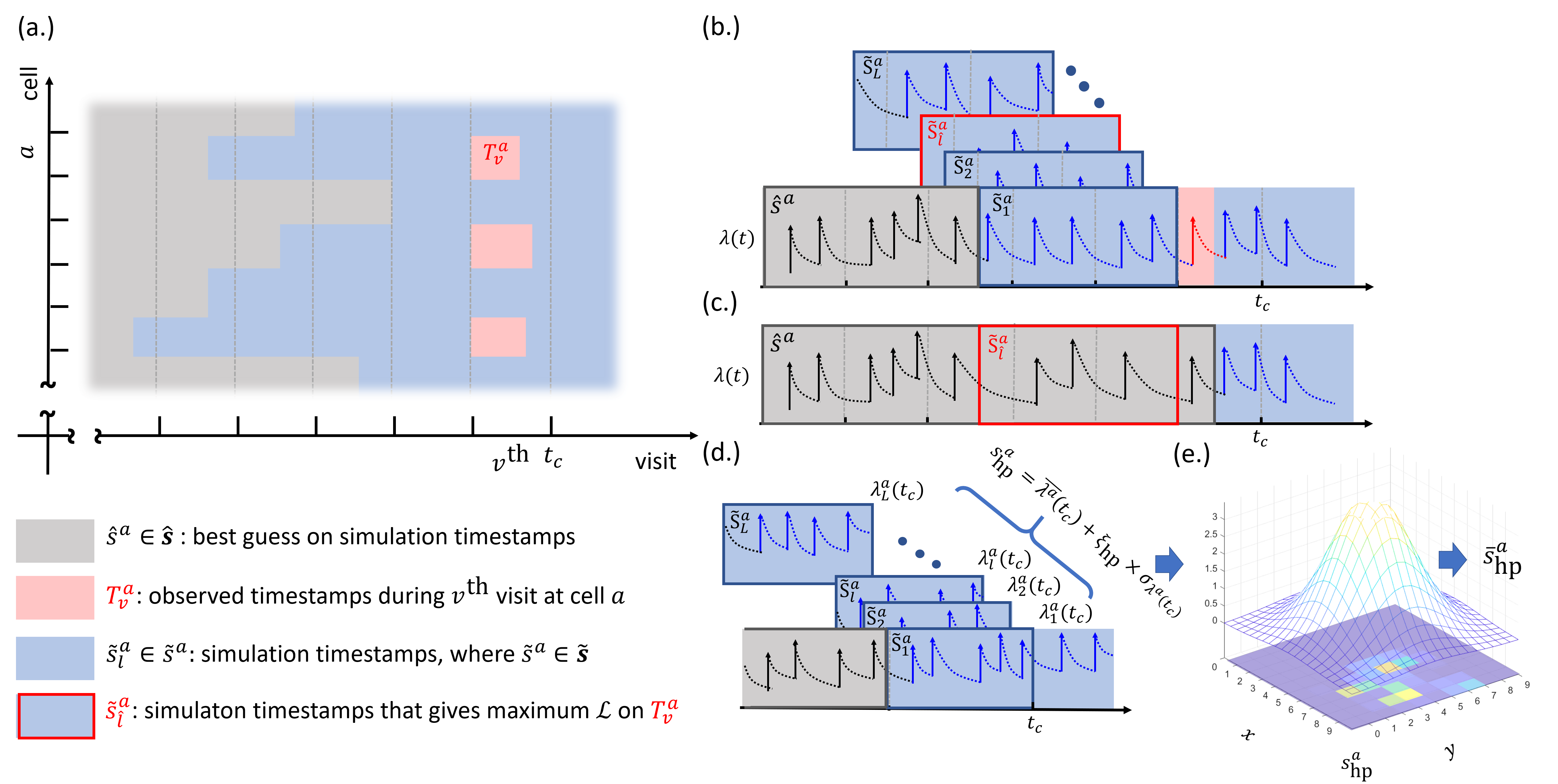
Figure 1: Overall framework on score $\overline{\boldsymbol{s}}_{\text{hp}}$ in $\mathop{\mathtt{HpSpUCB}}\limits$.

In Figure 1, we present the framework for determining a cell score $\overline{s}^{a}_{\text{hp}}$.

3.4 Baseline Methods

We will compare the Hawkes process MAB to several baseline algorithms. We also show in the subsequent section how to combine existing MAB strategies with the Hawkes process MAB to further improve performance.

3.4.1 Epsilon Greedy $\mathop{\mathtt{\epsilon\!\text{-}greedy}}\limits$:

The epsilon-greedy algorithm [16] separates trials into exploitation and exploration phases using a proportion of $\epsilon$ and $1-\epsilon$ visits respectively. We keep track of the average reward per visit for every cell after each visit, and then we visit the cells with the highest average reward during exploitation. During the exploration phase, we visit all the cells uniformly at random.

3.4.2 Upper Confidence Bound $\mathop{\mathtt{UCB1}}\limits$:

For upper confidence bound (UCB) algorithm [16], we construct an UCB on rewards so that the true value is always below the UCB with a high probability. We then pay visits to those promising cells with the highest UCB. The UCB of cell $a$ during visit $v$ is defined as a score, $s^{a}_{\text{ucb}}$, calculated as $s^{a}_{\text{ucb}}=\overline{r^{a}_{v}}+\zeta_{\text{ucb}}\sqrt{\frac{2\text{log}\,v}{n^{a}_{v}}}$ , where $\overline{r^{a}_{v}}$ is the average reward per visit and $n^{a}_{v}$ is the total number of visits up to visit $v$. The parameter $\zeta_{\text{ucb}}$ is to control how optimistic we are during the processes. Finally, after each visit, we update the scores $s^{a}_{\text{ucb}}$, and we select the top-$N$ cells with the highest score for the next visit.

3.4.3 Spatial Upper Confidence Bound $\mathop{\mathtt{SpUCB}}\limits$:

While the epsilon-greedy algorithm considers the cells with the largest mean value of rewards during exploitation, and the upper confidence bound (UCB) algorithm selects the most optimistic cells, neither considers the spatial relationship between the cells and the corresponding events. To introduce such geolocation information into MABs, Wu et al.[31] propose a space-aware UCB algorithm utilizing a Gaussian Process regression model ($\mathcal{GP}$)  [23] and building up a spatial UCB from the predicted expectation and uncertainty for each lever. After each visit, we collect the features of visited cells and their corresponding rewards, denoted as $\mathcal{X}$ and $\mathcal{Y}$, respectively. Together with previous collections, i.e., $\mathcal{X}=\mathcal{X}\cup\{\boldsymbol{x}_{a}|a\in\boldsymbol{a}\}$ and $\mathcal{Y}=\mathcal{Y}\cup\{r_{a}|a\in\boldsymbol{a}\}$, we train the $\mathcal{GP}$ regression model. In the $\mathcal{GP}$, we hold a prior assumption that the correlations between two cells $a$ and $a^{\prime}$ slowly decay following an exponential function of their distance. Thus, we select a radial basis kernel, $\mathbf{k}_{\text{RBF}}$, as the covariance of a prior distribution over the target functions. The kernel function $\mathbf{k}_{\text{RBF}}$ is calculated as follows: $\mathbf{k}_{\text{RBF}}(\boldsymbol{x}_{a},\boldsymbol{x}_{a^{\prime}})=\text{exp}\Big{(}\frac{-\|\boldsymbol{x}_{a},\boldsymbol{x}_{a^{\prime}}\|^{2}}{2\sigma_{\text{gp}}^{2}}\Big{)},$ where $\sigma_{\text{gp}}$ is a parameter that determines how far the correlation extends.

After each visit, we build the spatial UCB based on the prediction for each cell $a$ by looking at its $\zeta_{\text{gp}}$ predicted uncertainty above the expected mean, and we denote such a UCB as $s^{a}_{\text{gp}}$ (Equation 6). Here, $\boldsymbol{\mu}$ and $\boldsymbol{\sigma}$ are the predicted expectations and uncertainties given cell $a$ and $\zeta_{\text{gp}}$ governs how far we expend our upper confidence bound. Unlike $\mathop{\mathtt{\epsilon\!\text{-}greedy}}\limits$ and $\mathop{\mathtt{UCB1}}\limits$ in which only cells with the largest score are selected, the recommended cells are sampled for the next visit without replacement based on a probability distribution. Such probability distribution is calculated by a softmax function on $s^{a}_{\text{gp}}$ as in Equation 7, where $\tau_{\text{gp}}$ can be viewed as a temperature parameter that adjusts the exploitation and exploration ratio. We further denote such a baseline method as $\mathop{\mathtt{SpUCB}}\limits$.

$$\begin{aligned} s^{a}_{\text{gp}}=\boldsymbol{\mu}({\boldsymbol{x}_{a}})+\zeta_{\text{gp}}\boldsymbol{\sigma}({\boldsymbol{x}_{a}}).\\ \end{aligned}$$ (6)

$$\begin{aligned} p_{\text{gp}}^{a}=\frac{\text{exp}(s^{a}_{\text{gp}}/\tau_{\text{gp}})}{\sum_{a\in\mbox{$\mathop{\mathcal{A}}\limits$}}\text{exp}(s^{a}_{\text{gp}}/\tau_{\text{gp}})}.\\ \end{aligned}$$ (7)

3.5 Combining Hawkes Process Bandits with Existing Methods

Even though the upper confidence bound (UCB) built upon the Hawkes process ($\mathcal{HP}$) can track the event intensities, here we show how to improve its accuracy during the early stages of the multi-armed bandit (MAB) process. We combine the score from the UCB on intensities, $\overline{s}^{a}_{hp}$ in $\overline{\boldsymbol{s}}_{\text{hp}}$, with the score from the previously introduced method, that is, $s^{a}_{\text{ucb}}$ from $\mathop{\mathtt{UCB1}}\limits$ or $s^{a}_{\text{gp}}$ from $\mathop{\mathtt{SpUCB}}\limits$, respectively. We denote the combined score as $\widehat{s}^{a}$. Finally, we use a softmax function to calculate the probability $\widehat{p}^{a}$, and sample $N$ cells without replacement based on the probability for our next visit. We then denote our model as $\mathop{\mathtt{HpSpUCB}}\limits$.

More specifically, $\widehat{s}^{a}$ and $\widehat{p}^{a}$ are calculated as in Equation 8 and 9 where $\gamma$ governs how much we rely on intensities estimated through $\mathcal{HP}$s, and we can adjust our model based on how much the dataset itself contains a self-excitation pattern. Note that we define $\widehat{s}^{a}$ and $\widehat{p}^{a}$ from all cells as $\boldsymbol{\widehat{s}}$ and $\boldsymbol{\widehat{p}}$, respectively.

$$\begin{aligned} \widehat{s}^{a}=s^{a}+\gamma\overline{s}^{a}_{\text{hp}}.\end{aligned}$$ (8)

$$\begin{aligned} \widehat{p}^{a}=\frac{\text{exp}(\widehat{s}^{a}/\tau)}{\sum_{a\in\mbox{$\mathop{\mathcal{A}}\limits$}}\text{exp}(\widehat{s}^{a}/\tau)}.\end{aligned}$$ (9)

Based on the different choices of $s^{a}$ to combine with the $\mathcal{HP}$ component, we have different variations as our proposed models for comparison:

1. $\mathop{\mathtt{UCB1_{HpSp}}}\limits$ where $s^{a}=s^{a}_{\text{ucb}}$, that is, we combine $\overline{s}^{a}_{\text{hp}}$ with scores from $\mathop{\mathtt{UCB1}}\limits$;

2. $\mathop{\mathtt{UCB1_{Hp}}}\limits$ where $s^{a}=s^{a}_{\text{ucb}}$ while $\mathcal{GF}$ is not applied on $\boldsymbol{s}_{\text{hp}}$, that is, $\mathcal{GF}(\boldsymbol{s}_{\text{hp}}|0)$;

3. $\mathop{\mathtt{HpSpUCB}}\limits$ where $s^{a}=s^{a}_{\text{gp}}$, that is, we combine $\overline{s}^{a}_{\text{hp}}$ with scores from $\mathop{\mathtt{SpUCB}}\limits$.

Note that in $\mathop{\mathtt{UCB1_{Hp}}}\limits$, we remove the spatial smoothing so that we can compare with $\mathop{\mathtt{UCB1}}\limits$ to show the advantage of just adding the $\mathcal{HP}$ component. With $\mathop{\mathtt{HpSpUCB}}\limits$ and $\mathop{\mathtt{UCB1_{HpSp}}}\limits$, we can also compare when we choose different models to incorporate the proposed $\mathcal{HP}$ component. The overall MAB process of $\mathop{\mathtt{HpSpUCB}}\limits$ is presented in the algorithm 1, and algorithm 2 shows how our $\mathcal{HP}$ component plays its part in $\mathop{\mathtt{HpSpUCB}}\limits$.

Algorithm 1 Algorithm of $\mathop{\mathtt{HpSpUCB}}\limits$

1:procedure HpSpUCB( $\mbox{$\mathop{\mathcal{A}}\limits$},\,\gamma,\,\zeta_{\text{hp}},\,\zeta_{\text{gp}},\,\sigma_{\text{gp}},\,\tau$ )

2:    $X\leftarrow\emptyset$, $\boldsymbol{y}\leftarrow\emptyset$, $\boldsymbol{\hat{\mathcal{S}}}\leftarrow\emptyset$ , $\boldsymbol{\widetilde{\mathcal{S}}}\leftarrow\emptyset$, $t_{c}\leftarrow W$, $\boldsymbol{a}$ $\leftarrow$ select $N$ cells at random

3:    for $v=1$ to $V$ do $\triangleright$ MAB process

4:        $\boldsymbol{\mathcal{T}}\leftarrow\{\mathcal{T}_{v}^{a}|a\in\boldsymbol{a}\}$,  $\mathcal{X}\leftarrow\mathcal{X}\cup\{\boldsymbol{x}_{a}|a\in\boldsymbol{a}\}$,  $\mathcal{Y}\leftarrow\mathcal{Y}\cup\{r_{a}|a\in\boldsymbol{a}\}$

5:        $\boldsymbol{\mu},\boldsymbol{\sigma}\leftarrow\mathcal{GP}(\mathcal{X},\mathcal{Y}|\sigma_{\text{gp}})$ $\triangleright$ model and infer for $\mathcal{GP}$

6:        $\boldsymbol{s}_{\text{gp}}\leftarrow\{{s}^{a}_{\text{gp}}=\boldsymbol{\mu}({\boldsymbol{x}_{a}})+\zeta_{\text{gp}}\boldsymbol{\sigma}({\boldsymbol{x}_{a}})|a\in\mbox{$\mathop{\mathcal{A}}\limits$}\}$

7:        $\overline{\boldsymbol{s}}_{\text{hp}},\boldsymbol{\hat{\mathcal{S}}},\boldsymbol{\widetilde{\mathcal{S}}}\leftarrow\textsc{HpUCB}(\boldsymbol{\hat{\mathcal{S}}},\,\boldsymbol{\widetilde{\mathcal{S}}},\,\boldsymbol{a},\,\sigma_{\text{gp}},\,\zeta_{\text{hp}}\,t_{c},\,\mbox{$\mathop{\mathcal{A}}\limits$},\,\boldsymbol{\mathcal{T}})$ $\triangleright$ calculate scores of $\mathcal{HP}$s

8:        $\widehat{\boldsymbol{s}}\leftarrow\{\widehat{\boldsymbol{s}}^{a}=s^{a}_{\text{gp}}+\gamma\overline{s}^{a}_{\text{hp}}|a\in\mbox{$\mathop{\mathcal{A}}\limits$}\}$

9:        $\boldsymbol{\widehat{p}}\leftarrow$ apply softmax function on $\boldsymbol{\widehat{s}}$

10:        $\boldsymbol{a}\leftarrow$ sample $N$ cells based on probability $\boldsymbol{\widehat{p}}$

11:        $t_{c}\leftarrow(v+1)\times W$ $\triangleright$ update the current time $t_{c}$

12:    end for

13:end procedure

Algorithm 2 Calculation of $\overline{s}^{a}_{\text{hp}}$

1:function HpUCB($\boldsymbol{\hat{\mathcal{S}}},\,\boldsymbol{\widetilde{\mathcal{S}}},\,\boldsymbol{a},\,\sigma_{\text{gp}},\,\zeta_{\text{hp}}\,t_{c},\,\mbox{$\mathop{\mathcal{A}}\limits$},\,\boldsymbol{\mathcal{T}}$)

2:    for all $a\in\boldsymbol{a},\hat{\mathcal{S}^{a}}\in\boldsymbol{\hat{\mathcal{S}}},\widetilde{\mathcal{S}^{a}}\in\boldsymbol{\widetilde{\mathcal{S}}}$ do

3:        $\hat{l}\leftarrow\operatorname*{argmax}_{l}\mathcal{L}(\mathcal{T}_{v}^{a}|\theta_{l},\{\hat{\mathcal{S}}^{a},\widetilde{\mathcal{S}}^{a}_{l}\})$, where $\widetilde{\mathcal{S}}^{a}_{l}\in\widetilde{\mathcal{S}}^{a}$

4:        $\hat{\mathcal{S}^{a}}\leftarrow\{\hat{\mathcal{S}^{a}},\mathcal{S}^{a}_{\hat{l}},\mathcal{T}_{v}^{a}\}$

5:        $\Theta\leftarrow p(\mu,\alpha,\beta|\hat{\mathcal{S}_{a}})$

6:        $\widetilde{\mathcal{S}}^{a}\leftarrow\{\widetilde{\mathcal{S}}^{a}_{l}=\mathcal{HP}(\hat{\mathcal{S}}^{a}|\theta_{l})|\theta_{l}\in\Theta\}$

7:        update $\hat{\mathcal{S}^{a}}$ in $\boldsymbol{\hat{\mathcal{S}}}$ and $\widetilde{\mathcal{S}}^{a}$ in $\boldsymbol{\widetilde{\mathcal{S}}}$

8:    end for

9:    $\boldsymbol{s}_{\text{hp}}\leftarrow\{s^{a}_{\text{hp}}=\overline{\boldsymbol{\lambda}}^{a}(t_{c})+\zeta_{\text{hp}}\times{{\sigma}}_{{\boldsymbol{\lambda}^{a}(t_{c})}}|\;a\in\mbox{$\mathop{\mathcal{A}}\limits$}\}$,   where
     $\boldsymbol{\lambda}^{a}(t_{c})=\{\lambda_{l}^{a}(t_{c}|\theta_{l},\mathcal{T}^{a}_{l})|\;l=1,2,\cdots,L\}$ and $\mathcal{T}^{a}_{l}=\{\widetilde{\mathcal{S}}^{a}_{l}\cup\hat{\mathcal{S}^{a}}\ |\widetilde{\mathcal{S}}^{a}_{l}\in\widetilde{\mathcal{S}}^{a},\hat{\mathcal{S}}^{a}\in\boldsymbol{\hat{\mathcal{S}}}\}$

10:    $\overline{\boldsymbol{s}_{\text{hp}}}\leftarrow\mathcal{GF}(\boldsymbol{s}_{\text{hp}}|\sigma_{\text{gp}})$

11:    return $\overline{\boldsymbol{s}_{\text{hp}}},\boldsymbol{\hat{\mathcal{S}}},\,\boldsymbol{\widetilde{\mathcal{S}}}$

12:end function

4 Experiments

4.1 Datasets

4.1.1 Spatial-temporal Synthetic Data $\mathcal{D}_{\text{Syn}}$:

We first validate our methodology using a simulated Hawkes process ($\mathcal{HP}$) [20]. We generate a synthetic dataset by first simulating a Poisson process for initial immigrant events, of which the average number follows a Poisson distribution $\mathcal{P}(\eta T)$, and distribute them uniformly in space. Note that $\eta$ is the rate per second and $T$ is the total time span. Next, we generate a Poisson process recursively for each event in each generation by the following steps:

1. Draw a sample following a Poisson distribution $\mathcal{P}(\phi)$ as the number of offspring, where $\phi$ governs the average number of offspring that an event spawns;

2. Sample the waiting time between parent and offspring following an exponential distribution $\mathcal{E}(\omega)$;

3. Sample the spatial distance between parent and offspring event according to a normal distribution $\mathcal{N}(\sigma)$; and

4. Accept and record the event only when it is within the domain of time and space. We then go back step 1. and move on to the next recent event.

The simulation stops when all of a generation are outside $T$. We then denote these synthetic datasets as $\mathcal{D}_{\text{Syn}}$. In Figure 3, we present a realization of the synthetic data in $\mathcal{D}_{\text{Syn}}$ and show the top-20 largest clusters generated by the immigrants.

4.1.2 City of Houston 311 Service Requests $\mathcal{D}_{\text{Hry}}$:

We also apply the methodology to geolocated Houston 311 calls for service during the time period of hurricane Harvey in 2017. The dataset contains multiple types of requests with time and geo-location labels for when and where the request is made . The City of Houston 311 Service had recorded $77,601$ various 311 requests. Among all kinds of services, we focus on “flooding” events that contain complete timestamp, longitude and latitude information. Furthermore, we retain those events that happened between 08/23/2017 and 10/02/2017, e.g. after the hurricane had landed in Houston and before it dissipated. In total, there are $4,315$ 311 flooding events within Houston, Texas, where the range of latitude and longitude is (29.580562, 30.112111) and (-95.800000, -95.018014), respectively. We denote this dataset as $\mathcal{D}_{\text{Hry}}$. In Figure 3, we present the flooding events and color-code the timestamps. The color bar range starts at 00:00:00 on 08/23/2017, and we can also observe the pattern of disaster-related events, where the events are reported mostly in urban regions and mostly clustered in space and time.

Figure 2: Top-$20$ clusters in $\mathcal{D}_{\text{syn}}$. Different clusters are color-coded and the parameters under this simulation are $T=3.6\times 10^{6}$ seconds, $\eta=8\times 10^{-5}$, $\phi=0.99$, $\omega=10^{-4}$ and $\sigma=10^{-2}$.

Figure 3: Flooding Events in Houston $\mathcal{D}_{\text{Hry}}$. Each event is scaled and color-coded by its timestamps, and x-axis and y-axis represents the grid cell ID.

4.2 Experimental Protocol

Given a spatial domain, we first partition the range of longitude and latitude evenly into $10$ disjoint intervals, i.e., $X=10$ and $Y=10$. Thus, there are $100$ grid cells in total, and every event of interest can be mapped to a unique grid cell. In each visit, we select $5$ cells ($N=5$) to visit for a duration of $5$ hours ($W=18,000$) for synthetic datasets $\mathcal{D}_{\text{syn}}$ and $10$ cells ($N=10$) to visit for a duration of $20$ hours ($W=72,000$) for the 311 service request dataset $\mathcal{D}_{\text{Hry}}$. For each grid cell, we sample $50$ sets of parameters from the posterior distribution, i.e., $L=50$. Since the selected cells at the beginning may result in different decisions and performances in the whole MAB process, for every parameter in all the models, we run MAB processes for $10$ times with different initial visited cells, and we report the average of each evaluation score. Also, all parameters of the models are studied through an extensive grid search, and the best performances are reported for the model comparison. For the sake of reproducibility, all datasets and the source code are made publicly available in an anonymized repository .

4.3 Evaluation Metrics

We measure the performance of competing models by the cumulative reward, that is, the number of the observed events captured in visited cells. To compare the performances between different datasets in $\mathcal{D}_{\text{syn}}$, we then normalize the total reward by the number of the total events and we denote it as $\mathop{\mathtt{\overline{reward}}}\limits$. At each visit, models generate a short ranked list for the next visit. Based on the ranked lists, we can also evaluate the models through different ranking and recommendation metrics. One popular metric to evaluate the ranking quality is the normalized discounted cumulative gain (NDCG) [30]. We then calculate the NDCG at $N$ for each visit, where $N$ is the number of visited cells. The relevance value (i.e., gain) at cell $\mathop{a}\limits$ and visit $v$ is then defined as the number of events, i.e., $|\mathcal{T}^{a}_{v}|$. Finally, we take the average across all the visits and denote it as $\mathop{\mathtt{NDCG}}\limits$.

From the recommendation point of view, we are interested in how many cells recommended by the models would actually contain events during our visit. We first consider that a cell is relevant if there are one or more events during the visit. We then evaluate such recommendation quality through the modified reciprocal hit rank [21], denoted as $\mathop{\mathtt{mRHR}}\limits$ for evaluation. Modified reciprocal hit rank is a modified version of average reciprocal hit rank (ARHR), which is feasible for ranked recommendation evaluations where there are multiples relevant items (i.e., relevant cells). It can be calculated as follows:

$$\begin{aligned} &\mbox{$\mathop{\mathtt{mRHR}}\limits$}=\frac{1}{\bigm{|}\boldsymbol{g}\bigm{|}}\sum\limits_{i=1}^{N}\frac{\mathtt{h}_{i}}{\mathtt{r}_{i}},\text{where }\mathtt{h}_{i}=\begin{cases}1\!&\!\!\text{if }a_{i}\in\boldsymbol{g}\\ 0\!&\!\!\text{if }a_{i},\notin\boldsymbol{g}\\ \end{cases},\mathtt{r}_{i}=\begin{cases}\mathtt{r}_{i-1}\!\!\!\!&\!\text{if }\mathtt{h}_{i-1}=1\\ \mathtt{r}_{i-1}\!+\!1\!\!\!\!&\!\text{if }\mathtt{h}_{i-1}=0,\\ \end{cases}\\ \end{aligned}$$ (10)

where $\boldsymbol{g}$ is a list of relevant cells; $a_{i}\in\boldsymbol{a}$; $\mathtt{h}$ and $\mathtt{r}$ represent hit and rank, respectively; and each hit is rewarded based on its position in the ranked list.

We also evaluate the models on recall, precision, F1 score [14], normalized precision, and average normalized precision [7]. Recall, denoted as $\mathop{\mathtt{rec}}\limits$, measures the power of the models to discover high-risk cells. It is the fraction of the relevant cells that are successfully recommended. Precision, denoted as $\mathop{\mathtt{prc}}\limits$, measures how precise the recommendation list is. F1 score, denoted as $\mathop{\mathtt{f1}}\limits$, is simply the harmonic mean between $\mathop{\mathtt{rec}}\limits$ and $\mathop{\mathtt{prc}}\limits$. Note that the maximal $\mathop{\mathtt{prc}}\limits$ can be less than 1 since the relevant cells can be less than $N$. Therefore, we also calculate normalized precision, denoted as $\mathop{\overline{{\mathtt{prc}}}}\limits$, by dividing $\mathop{\mathtt{prc}}\limits$ by the maximal $\mathop{\mathtt{prc}}\limits$ where maximal $\mathop{\mathtt{prc}}\limits$ happens when $\boldsymbol{a}$ is optimal. Finally, we compare using average precision $\mathop{\overline{{\mathtt{{Aprc}}}}}\limits$ calculated as: $\mbox{$\mathop{\overline{{\mathtt{{Aprc}}}}}\limits$}=\frac{1}{|\boldsymbol{g}|}\sum_{k=1}^{N}\mbox{$\mathop{\overline{{\mathtt{prc}}}}\limits$}@k$ where $\mbox{$\mathop{\overline{{\mathtt{prc}}}}\limits$}@k$ is when we only consider the top $k$ cells in the recommended list $\boldsymbol{a}$.

4.4 Experimental Results

4.4.1 Performances on the synthetic datasets $\mathcal{D}_{\text{syn}}$:

Figure 4: Performance on $\mathop{\mathtt{\overline{reward}}}\limits$ on $\mathcal{D}_{\text{syn}}$ under different simulation scenarios with various of $\omega,\phi$ and $\sigma$. We run simulations by changing only one of the parameters at a time and the other parameters, i.g., $\omega,\phi$ and $\sigma$, are fixed at $10^{-4},0.99$ and $10^{-2}$, respectively.

We compare the performance of our model $\mathop{\mathtt{HpSpUCB}}\limits$ against competitive baseline methods, $\mathop{\mathtt{UCB1}}\limits$ and $\mathop{\mathtt{SpUCB}}\limits$, in terms of $\mathop{\mathtt{\overline{reward}}}\limits$ when applied to synthetic datasets $\mathcal{D}_{\text{syn}}$ with different spatio-temporal patterns. The results of $\mathop{\mathtt{\overline{reward}}}\limits$ are presented in Figure 4. Figure 4 demonstrates the $\mathop{\mathtt{\overline{reward}}}\limits$ under different $\omega$, while $\phi$ and $\sigma$ while fixing the other parameters. Our $\mathop{\mathtt{HpSpUCB}}\limits$ outperforms the other baselines by a large margin, with the exception of when the process is approximately stationary over moderate time scales. This occurs when $\phi$ or $\omega$ are too small or too large relative to the time scale of a visit, and in this scenario the Hawkes process loses its advantage over stationary models.

4.4.2 Performances on Houston 311 Service Requests $\mathcal{D}_{\text{Hry}}$:

Table 1: Best Performance on $\mathcal{D}_{\text{Hry}}$

Model	$\mathop{\mathtt{\overline{reward}}}\limits$	$\mathop{\mathtt{NDCG}}\limits$	$\mathop{\mathtt{mRHR}}\limits$	$\mathop{\mathtt{rec}}\limits$	$\mathop{\mathtt{prc}}\limits$	$\mathop{\mathtt{f1}}\limits$	$\mathop{\overline{{\mathtt{prc}}}}\limits$	$\mathop{\overline{{\mathtt{{Aprc}}}}}\limits$
$\mathop{\mathtt{\epsilon\!\text{-}greedy}}\limits$	0.1766	0.2224	0.1345	0.1758	0.2152	0.1928	0.2719	0.3285
$\mathop{\mathtt{UCB1}}\limits$	0.1897	0.2917	0.1669	0.2032	0.2547	0.2233	0.3106	0.3943
$\mathop{\mathtt{UCB1_{Hp}}}\limits$	0.2122	0.3198	0.1880	0.2286	0.2649	0.2367	0.3284	0.4460
$\mathop{\mathtt{UCB1_{HpSp}}}\limits$	0.2181	0.3502	0.2016	0.2404	0.2679	0.2491	0.3413	0.4613
$\mathop{\mathtt{SpUCB}}\limits$	0.2473	0.3440	0.1963	0.2489	0.2956	0.2697	0.3728	0.4487
$\mathop{\mathtt{HpSpUCB}}\limits$	0.2546	0.3584	0.2087	0.2633	0.3074	0.2834	0.3920	0.4661

Table 1 presents the best performance according to each evaluation metric of the models applied the Houston 311 call dataset $\mathcal{D}_{\text{Hry}}$. In general, our model $\mathop{\mathtt{HpSpUCB}}\limits$ outperforms all of the other baselines in every metric that we evaluate. In particular, by adding an event intensity tracking mechanism in the decision-making, the performance of $\mathop{\mathtt{HpSpUCB}}\limits$ is better than $\mathop{\mathtt{SpUCB}}\limits$ both on reward optimization and high-risk cell recommendation. In terms of $\overline{\text{reward}}$, the proposed $\mathop{\mathtt{HpSpUCB}}\limits$ outperforms the second-best model, $\mathop{\mathtt{SpUCB}}\limits$, by $2.95\%$ while it also surpasses $\mathop{\mathtt{UCB1_{HpSp}}}\limits$ in $\mathop{\mathtt{NDCG}}\limits$ and $\mathop{\mathtt{mRHR}}\limits$ by $2.34\%$ and $3.52\%$ from the ranking perspective. From the high-risk cell retrieval point of view, $\mathop{\mathtt{HpSpUCB}}\limits$ consistently outperforms $\mathop{\mathtt{SpUCB}}\limits$ in $\mathop{\mathtt{rec}}\limits$, $\mathop{\mathtt{prc}}\limits$, $\mathop{\mathtt{f1}}\limits$, and normalized precision $\mathop{\overline{{\mathtt{prc}}}}\limits$ by $5.79\%$, $3.99\%$, $5.08\%$, and $5.15\%$, respectively. In terms of normalized precision, $\mathop{\overline{{\mathtt{{Aprc}}}}}\limits$, $\mathop{\mathtt{HpSpUCB}}\limits$ is still better than its competitive opponent $\mathop{\mathtt{UCB1_{HpSp}}}\limits$ by $1.04\%$. These improvements in accuracy illustrate $\mathop{\mathtt{HpSpUCB}}\limits$’s ability to recall events through event intensity tracking and provide better recommendations on the high-risk cells. By combining the method with the existing algorithm, stationary patterns of events are also taken into consideration and the combined model strikes a good balance between the $\mathcal{HP}$ component and the other UCB component.

Compared to $\mathop{\mathtt{UCB1}}\limits$, both $\mathop{\mathtt{UCB1_{Hp}}}\limits$ and $\mathop{\mathtt{UCB1_{HpSp}}}\limits$ contain the proposed $\mathcal{HP}$ component, while for $\mathop{\mathtt{UCB1_{Hp}}}\limits$, the spatial smoothing is removed. We can see from Table 1 that $\mathop{\mathtt{UCB1_{HpSp}}}\limits$ consistently outperforms both $\mathop{\mathtt{UCB1_{Hp}}}\limits$ and $\mathop{\mathtt{UCB1}}\limits$ in all of the evaluation metrics. $\mathop{\mathtt{UCB1_{HpSp}}}\limits$ and $\mathop{\mathtt{UCB1_{Hp}}}\limits$ out perform $\mathop{\mathtt{UCB1}}\limits$ by a large margin in both reward-based and ranking quality based evaluation. These results suggest that our proposed $\mathcal{HP}$ component is out-performing traditional stationary MAB algorithms like $\mathop{\mathtt{UCB1}}\limits$ by tracking the space-time dynamic reward distribution.

Table 2: Performance on $\mathcal{D}_{\text{Hry}}$ Corresponding to Best $\overline{\text{reward}}$

Model	best $\mathop{\mathtt{\overline{reward}}}\limits$					best $\mathop{\mathtt{NDCG}}\limits$
	$\mathop{\mathtt{NDCG}}\limits$	$\mathop{\mathtt{mRHR}}\limits$	$\mathop{\mathtt{f1}}\limits$	$\mathop{\overline{{\mathtt{{Aprc}}}}}\limits$		$\mathop{\mathtt{\overline{reward}}}\limits$	$\mathop{\mathtt{mRHR}}\limits$	$\mathop{\mathtt{f1}}\limits$	$\mathop{\overline{{\mathtt{{Aprc}}}}}\limits$
$\mathop{\mathtt{\epsilon\!\text{-}greedy}}\limits$	0.2125	0.1254	0.1790	0.2862		0.1615	0.1345	0.1928	0.3285
$\mathop{\mathtt{UCB1}}\limits$	0.2714	0.1581	0.2233	0.3460		0.1810	0.1669	0.2120	0.3943
$\mathop{\mathtt{UCB1_{Hp}}}\limits$	0.3042	0.1697	0.2295	0.3956		0.1987	0.1880	0.2319	0.4460
$\mathop{\mathtt{UCB1_{HpSp}}}\limits$	0.3349	0.1850	0.2409	0.4323		0.2061	0.2016	0.2481	0.4613
$\mathop{\mathtt{SpUCB}}\limits$	0.3366	0.1912	0.2697	0.4125		0.2467	0.1963	0.2675	0.4487
$\mathop{\mathtt{HpSpUCB}}\limits$	0.3070	0.1717	0.2475	0.3819		0.2492	0.2087	0.2834	0.4661

In table 2, we present results for the evaluation metrics $\mathop{\mathtt{\overline{reward}}}\limits$, $\mathop{\mathtt{NDCG}}\limits$, $\mathop{\mathtt{mRHR}}\limits$, $\mathop{\mathtt{f1}}\limits$ and $\mathop{\overline{{\mathtt{prc}}}}\limits$ when choosing the model parameters with respect to the best $\mathop{\mathtt{\overline{reward}}}\limits$ and $\mathop{\mathtt{NDCG}}\limits$ respectively. When hyper-parameters are selected based on the best $\mathop{\mathtt{\overline{reward}}}\limits$, $\mathop{\mathtt{HpSpUCB}}\limits$ performs better than $\mathop{\mathtt{SpUCB}}\limits$ according to table 1. However, $\mathop{\mathtt{SpUCB}}\limits$ performs better than all the other models. This suggests that there may be a trade-off between $\mathop{\mathtt{\overline{reward}}}\limits$ and other metrics. When we optimize the total number of events, we may only focus on the spike in certain grids in terms of the number of events, but sacrifice the ranking quality of the model.

Figure 5: $\mathop{\mathtt{\overline{reward}}}\limits$ through visits

In Figure 5, we present $\mathop{\mathtt{\overline{reward}}}\limits$ throughout the visits in the MAB process. Here, we can see that in the early visits, models with the $\mathcal{HP}$ component (e.g. $\mathop{\mathtt{HpSpUCB}}\limits$, $\mathop{\mathtt{UCB1_{Hp}}}\limits$ and $\mathop{\mathtt{UCB1_{HpSp}}}\limits$) have similar results as their predecessors ($\mathop{\mathtt{SpUCB}}\limits$ and $\mathop{\mathtt{UCB1}}\limits$). However, as we collect more information and observe more events, the variance is reduced in the posterior distributions for the Hawkes process model parameters, and the intensity estimates become more precise. At this later stage in the MAB process, the $\mathcal{HP}$ components in $\mathop{\mathtt{HpSpUCB}}\limits$, $\mathop{\mathtt{UCB1_{Hp}}}\limits$ and $\mathop{\mathtt{UCB1_{HpSp}}}\limits$ boost the performance. In Figure 8 and Figure 8, we compare the number of flooding events and the average number of total visits for each grid cell from the best $\mathop{\mathtt{\overline{reward}}}\limits$ in our model $\mathop{\mathtt{HpSpUCB}}\limits$. We can see that the number of flooding events in the cells is highly correlated to the average number of visits at the end of the MAB process. This suggests that after the trial of exploration, eventually, our $\mathop{\mathtt{HpSpUCB}}\limits$ will learn those cells that are most susceptible to flooding and focus on these in terms of exploitation. Figure 8 is the snapshot of the flooding map in cell (4,1), that $\mathop{\mathtt{HpSpUCB}}\limits$ visits the most. It is located by the watershed of The Brays Bayou, a slow-moving river which is notorious for its flooding history in Houston, Texas. This also indicates that $\mathop{\mathtt{HpSpUCB}}\limits$ can identify hotspot areas for further investigation.

Figure 6: Number of events

Figure 7: Number of visits

Figure 8: Street Map on (4,1)

In Table 4 and Table 4, we present the parameter study of $\mathop{\mathtt{HpSpUCB}}\limits$ on
$\mathcal{D}_{\text{Hry}}$ in terms of $\mathop{\mathtt{\overline{reward}}}\limits$. We mainly focus on $\gamma$, $\sigma_{\text{gp}}$, $\tau$, and $\zeta_{\text{gp}}$, which have a more significant influence on $\mathop{\mathtt{HpSpUCB}}\limits$ in $\mathcal{D}_{\text{Hry}}$. The best $\mathop{\mathtt{\overline{reward}}}\limits$ sits in a window for both $\gamma$ and $\sigma_{\text{gp}}$, which control the $\mathcal{HP}$ contribution and the spatial correlation, respectively. This result shows that both the $\mathcal{HP}$ component and traditional spatial MAB component contribute to the performance, and $\mathop{\mathtt{HpSpUCB}}\limits$ can adapt to the spatial correlations in the events through the Gaussian kernel and Gaussian filter. In Table 4, the best $\mathop{\mathtt{\overline{reward}}}\limits$ is also located in a range for $\tau$ and $\zeta_{\text{gp}}$, which are in charge of the temperature in the softmax function for sampling the cells and the weight of upper confidence bound (UCB) on the average reward. These results suggest that $\mathop{\mathtt{HpSpUCB}}\limits$ also addresses the trade-off between exploitation and exploration.

Table 3: Parameter Study on $\gamma$ and $\sigma_{\text{gp}}$

	0.01	0.1	0.5	1	10
0.1	0.1441	0.1663	0.1660	0.1450	0.1502
0.5	0.2078	0.2190	0.1868	0.1909	0.1446
1	0.1940	0.1928	0.2546	0.2057	0.1513
5	0.2237	0.2087	0.2010	0.2208	0.1907

Table 4: Parameter Study of $\zeta_{\text{gp}}$ and $\tau$

	0.0001	0.001	0.01	0.1	1
0.01	0.1236	0.2170	0.1737	0.1075	0.0534
0.1	0.1225	0.2092	0.2213	0.0769	0.0554
1	0.1428	0.1874	0.2546	0.0908	0.0511
10	0.1477	0.1847	0.2417	0.0696	0.0561

5 Conclusion

We introduced a novel framework $\mathop{\mathtt{HpSpUCB}}\limits$ that integrates Bayesian Hawkes processes ($\mathcal{HP}$) with a spatial multi-armed bandit (MAB) algorithm to forecast spatio-temporal events and detect hotspots where disaster search and rescue efforts may be directed. In particular, the model forecasts synthetic events between each visit to a geographical area to infer the intensity in the gap between between visits. An upper confidence bound on the estimated intensity is then built for dynamic event tracking. We then apply a Gaussian filter to incorporate the spatial relationships between grid cells. We compared our $\mathop{\mathtt{HpSpUCB}}\limits$ against competitive baselines through extensive experiments. In simulated synthetic datasets with space-time clustering, our $\mathop{\mathtt{HpSpUCB}}\limits$ improves upon existing stationary spatial MAB algorithms. In the case of Houston 311 service requests during hurricane Harvey, $\mathop{\mathtt{HpSpUCB}}\limits$ outperforms the baseline models considered in terms of a variety of metrics including total reward and ranking quality. Overall, with the $\mathcal{HP}$ component, we can enhance the performance of MAB algorithms. In the future, more contextual information may be used to further improve point process MAB algorithms. Furthermore, other types of point processes (log-Gaussian Cox processes, self-avoiding processes, etc.) may be combined with multi-armed bandits to solve other types of applications.

6 Acknowledgements

This research was supported by NSF grants SCC-1737585 and ATD-1737996.

References

- [1] Bacry, E., Bompaire, M., Gaïffas, S., Poulsen, S.: Tick: a python library for statistical learning, with a particular emphasis on time-dependent modelling. arXiv preprint arXiv:1707.03003 (2017)
- [2] Bacry, E., Mastromatteo, I., Muzy, J.F.: Hawkes processes in finance. Market Microstructure and Liquidity 1(01), 1550005 (2015)
- [3] Chakrabarti, D., Kumar, R., Radlinski, F., Upfal, E.: Mortal multi-armed bandits. In: Advances in neural information processing systems. pp. 273–280 (2009)
- [4] Cheong, F., Cheong, C.: Social media data mining: A social network analysis of tweets during the 2010-2011 australian floods. PACIS 11, 46–46 (2011)
- [5] Chiang, W.H., Yuan, B., Li, H., Wang, B., Bertozzi, A.L., Carter, J., Ray, B., Mohler, G.: Sos-ew : System for overdose spike early warning using drug mover ’ s distance-based hawkes processes. In: ECML PKDD 2019 Workshops (2019)
- [6] Chu, W., Li, L., Reyzin, L., Schapire, R.: Contextual bandits with linear payoff functions. In: Proceedings of the Fourteenth International Conference on Artificial Intelligence and Statistics. pp. 208–214 (2011)
- [7] Cormack, G.V., Lynam, T.R.: Statistical precision of information retrieval evaluation. In: Proceedings of the 29th annual international ACM SIGIR conference on Research and development in information retrieval. pp. 533–540. ACM (2006)
- [8] Durand, A., Achilleos, C., Iacovides, D., Strati, K., Mitsis, G.D., Pineau, J.: Contextual bandits for adapting treatment in a mouse model of de novo carcinogenesis. In: Machine Learning for Healthcare Conference. pp. 67–82 (2018)
- [9] Eckles, D., Kaptein, M.: Thompson sampling with the online bootstrap. arXiv preprint arXiv:1410.4009 (2014)
- [10] Fox, E.W., Schoenberg, F.P., Gordon, J.S., et al.: Spatially inhomogeneous background rate estimators and uncertainty quantification for nonparametric hawkes point process models of earthquake occurrences. The Annals of Applied Statistics 10(3), 1725–1756 (2016)
- [11] Gopalan, A., Mannor, S., Mansour, Y.: Thompson sampling for complex online problems. In: International Conference on Machine Learning. pp. 100–108 (2014)
- [12] Goswami, S., Chakraborty, S., Ghosh, S., Chakrabarti, A., Chakraborty, B.: A review on application of data mining techniques to combat natural disasters. Ain Shams Engineering Journal 9(3), 365–378 (2018)
- [13] Gupta, N., Granmo, O.C., Agrawala, A.: Thompson sampling for dynamic multi-armed bandits. In: 2011 10th International Conference on Machine Learning and Applications and Workshops. vol. 1, pp. 484–489. IEEE (2011)
- [14] Hripcsak, G., Rothschild, A.S.: Agreement, the f-measure, and reliability in information retrieval. Journal of the American Medical Informatics Association 12(3), 296–298 (2005)
- [15] Krause, A., Ong, C.S.: Contextual gaussian process bandit optimization. In: Advances in neural information processing systems. pp. 2447–2455 (2011)
- [16] Kuleshov, V., Precup, D.: Algorithms for multi-armed bandit problems. arXiv preprint arXiv:1402.6028 (2014)
- [17] Li, L., Chu, W., Langford, J., Schapire, R.E.: A contextual-bandit approach to personalized news article recommendation. In: Proceedings of the 19th international conference on World wide web. pp. 661–670 (2010)
- [18] Merz, B., Kreibich, H., Lall, U.: Multi-variate flood damage assessment: a tree-based data-mining approach. Natural Hazards and Earth System Sciences (NHESS) 13(1), 53–64 (2013)
- [19] Mohler, G.O., Short, M.B., Brantingham, P.J., Schoenberg, F.P., Tita, G.E.: Self-exciting point process modeling of crime. Journal of the American Statistical Association 106(493), 100–108 (2011)
- [20] Møller, J., Rasmussen, J.G.: Perfect simulation of hawkes processes. Advances in applied probability 37(3), 629–646 (2005)
- [21] Peker, S., Kocyigit, A.: mrhr: a modified reciprocal hit rank metric for ranking evaluation of multiple preferences in top-n recommender systems. In: International Conference on Artificial Intelligence: Methodology, Systems, and Applications. pp. 320–329. Springer (2016)
- [22] Qin, L., Chen, S., Zhu, X.: Contextual combinatorial bandit and its application on diversified online recommendation. In: Proceedings of the 2014 SIAM International Conference on Data Mining. pp. 461–469. SIAM (2014)
- [23] Rasmussen, C., Williams, C.: Gaussian processes for machine learning the mit press (2006)
- [24] Rasmussen, J.G.: Bayesian inference for hawkes processes. Methodology and Computing in Applied Probability 15(3), 623–642 (2013)
- [25] Roberts, G.O., Gelman, A., Gilks, W.R., et al.: Weak convergence and optimal scaling of random walk metropolis algorithms. The annals of applied probability 7(1), 110–120 (1997)
- [26] Smith, W.R., Stephens, K.K., Robertson, B., Li, J., Murthy, D.: Social media in citizen-led disaster response: Rescuer roles, coordination challenges, and untapped potential. In: Proceedings of the… International ISCRAM Conference (2018)
- [27] Tehrany, M.S., Pradhan, B., Jebur, M.N.: Spatial prediction of flood susceptible areas using rule based decision tree (dt) and a novel ensemble bivariate and multivariate statistical models in gis. Journal of Hydrology 504, 69–79 (2013)
- [28] Tokic, M., Palm, G.: Value-difference based exploration: adaptive control between epsilon-greedy and softmax. In: Annual Conference on Artificial Intelligence. pp. 335–346. Springer (2011)
- [29] Tran-Thanh, L., Chapman, A., de Cote, E.M., Rogers, A., Jennings, N.R.: Epsilon–first policies for budget–limited multi-armed bandits. In: Twenty-Fourth AAAI Conference on Artificial Intelligence (2010)
- [30] Wang, Y., Wang, L., Li, Y., He, D., Chen, W., Liu, T.Y.: A theoretical analysis of ndcg ranking measures. In: Proceedings of the 26th annual conference on learning theory (COLT 2013). vol. 8, p. 6 (2013)
- [31] Wu, C.M., Schulz, E., Speekenbrink, M., Nelson, J.D., Meder, B.: Mapping the unknown: The spatially correlated multi-armed bandit. bioRxiv p. 106286 (2017)
- [32] Zhou, L., Brunskill, E.: Latent contextual bandits and their application to personalized recommendations for new users. arXiv preprint arXiv:1604.06743 (2016)