Tree-AMP: Compositional Inference with Tree Approximate Message Passing

Abstract

We introduce Tree-AMP, standing for Tree Approximate Message Passing, a python package for compositional inference in high-dimensional tree-structured models. The package provides a unifying framework to study several approximate message passing algorithms previously derived for a variety of machine learning tasks such as generalized linear models, inference in multi-layer networks, matrix factorization, and reconstruction using non-separable penalties. For some models, the asymptotic performance of the algorithm can be theoretically predicted by the state evolution, and the measurements entropy estimated by the free entropy formalism. The implementation is modular by design: each module, which implements a factor, can be composed at will with other modules to solve complex inference tasks. The user only needs to declare the factor graph of the model: the inference algorithm, state evolution and entropy estimation are fully automated. The source code is publicly available at https://github.com/sphinxteam/tramp and the documentation at https://sphinxteam.github.io/tramp.docs.

1 Introduction

Probabilistic models have been used in many applications, as diverse as scientific data analysis, coding, natural language and signal processing. They also offer a powerful framework (Bishop, 2013) to several challenges in machine learning: dealing with uncertainty, choosing hyper-parameters, causal reasoning and model selection. However, the difficulty of deriving and implementing approximate inference algorithms for each new model may have hindered the wider adoption of Bayesian methods. The probabilistic programming approach seeks to make Bayesian inference as user friendly and streamlined as possible: ideally the user would only need to declare the probabilistic model and run an inference engine. Several probabilistic programming frameworks have been proposed, well suited for different contexts and leveraging variational inference or sampling methods to automate inference. To give a few examples, pomegranate (Schreiber, 2018) fits probabilistic models using maximum likelihood. Church (Goodman et al., 2008) and successors are universal languages for representing generative models. Infer.NET (Minka et al., 2018) implements several message passing algorithms such as Expectation Propagation. Stan (Carpenter et al., 2017) uses Hamiltonian Monte Carlo, while Anglican (Wood et al., 2014) uses particle MCMC as the sampling method. Turing (Ge et al., 2018) offers a Julia implementation. Recently, Edward (Tran et al., 2016) and Pyro (Bingham et al., 2018) tackle deep probabilistic problems, scaling inference up to large data and complex models.

In this paper, we present Tree-AMP (Tree Approximate Message Passing). In the current rich software ecosystem, Tree-AMP aims to fill a particular niche: using message passing algorithms with theoretical guarantees of performance in specific asymptotic settings. As will be detailed in Section 2, Tree-AMP uses the Expectation Propagation (EP) algorithm (Minka, 2001a) as its inference engine, which is also implemented by Infer.NET. Application-wise, for inference in statistical models or Bayesian machine learning tasks, the scope of Tree-AMP is very limited compared to the Infer.NET package. Indeed Tree-AMP is restricted to models like the ones presented in Figure 1, that is tree-structured factor graphs connecting high-dimensional variables, while Infer.NET can be applied to generic factor graphs with variables of arbitrary dimensions and types. However for the models considered in Figure 1, under specific asymptotic settings, Tree-AMP offers an in-depth theoretical analysis of its performance as will be detailed in Section 3: its errors can be predicted using the state evolution formalism, the free entropy formalism further predicts when the algorithm achieves or not the Bayes-optimal performance and also allows to estimate information theoretic quantities. For this reason, we believe the Tree-AMP package should be of special interest to theoretical researchers seeking a better understanding of EP/AMP algorithms. As an alternative to Tree-AMP let us mention the Vampyre package that allows inference in multi-layer networks (Fletcher et al., 2018).

There is a long history behind message passing (Yedidia and Freeman, 2001; Mézard and Montanari, 2009), approximate message passing (AMP) (Donoho et al., 2009) and vector approximate message passing (VAMP) (Schniter et al., 2017), that we shall discuss later on. As exemplified in the context of compressed sensing, the AMP algorithm has a fundamental property: its performance on random instances in the high-dimensional limit, measured by the mean squared error on the signals, can be rigorously predicted by the so-called state evolution (Donoho et al., 2009; Bayati and Montanari, 2011), a rigorous version of the physicists "cavity method" (Mézard et al., 1987). These performances can be shown, in some cases, to reach the Bayes optimal one in polynomial time (Barbier et al., 2016; Reeves and Pfister, 2016), quite a remarkable feat! More recently, variant of the AMP approach has been developed with (some) correlated data and matrices (Schniter et al., 2017; Ma and Ping, 2017), again with guarantees of optimally in some cases (Barbier et al., 2018; Gerbelot et al., 2020). These approaches are intimately linked with the Expectation Propagation algorithm (Minka, 2001a) and the Expectation Consistency framework (Opper and Winther, 2005a).

(a)         

(b)          

(c)         

(d)         

(e)         

Figure 1: Tree-structured models. (a) Generalized linear model with separable prior $p_{0}(x)$, separable likelihood $p_{\text{out}}(y|z)$ and linear channel $z=Wx$. (b) Reconstruction using a sparse gradient prior where sparsity is enforced by the Gauss-Bernoulli prior $\mathcal{N}_{\rho}=[1-\rho]\delta+\rho\mathcal{N}$. (c) Low-rank matrix factorization with separable priors $p_{U}$ and $p_{V}$, separable likelihood $p_{\text{out}}(Y|Z)$ and factorization $Z=\frac{UV^{\intercal}}{\sqrt{N}}$. (d) Multi-layer network with activation functions $a_{l}=\sigma_{l}(z_{l})$ and linear channels $z_{l}=W_{l}a_{l-1}$. (e) Committee machine with three experts.

The state evolution and the Bayes optimal guarantees were extended to a wide variety of models including for instance generalized linear models (GLM) (Rangan, 2011; Barbier et al., 2019), matrix factorization (Rangan and Fletcher, 2012; Deshpande and Montanari, 2014; Dia et al., 2016; Lesieur et al., 2017), committee machines (Aubin et al., 2018), optimization with non separable penalties (such as total variation) (Som and Schniter, 2012; Metzler et al., 2015; Tan et al., 2015; Manoel et al., 2018), inference in multi-layer networks (Manoel et al., 2017; Fletcher et al., 2018; Gabrié et al., 2018) and even arbitrary trees of GLMs (Reeves, 2017). In all these cases, the entropy of the system in the high dimensional limit can be obtained as the minimum of the so-called free entropy potential (Yedidia and Freeman, 2001; Yedidia et al., 2005; Krzakala et al., 2014) and this allows the computation of interesting information theoretic quantities such as the mutual information between layers in a neural network (Gabrié et al., 2018). Furthermore, the global minimizer of the free entropy potential corresponds to the minimal mean squared error, which allows to determine fundamental limits to inference. Interestingly, the mean squared error achieved by AMP, predicted by the state evolution, is a stationary point of the same free entropy potential, which allows for an interesting interpretation of when the algorithm actually works (Zdeborová and Krzakala, 2016) in terms of phase transitions.

Unfortunately the development of AMP algorithms faced the same caveat as probabilistic modeling: for each new model, the AMP algorithm and the associated theory (free entropy and state evolution) had to be derived and implemented separately, which can be time-consuming. However, a key observation is that the factor graphs (Kschischang et al., 2001) for all the models mentioned above are tree-structured as illustrated in Figure 1. Each factor corresponds to an elementary inference problem that can be solved analytically or approximately. The Tree-AMP python package offers a unifying framework for all the models discussed above and extends to arbitrary tree-structured models. Similar to other probabilistic programming frameworks, the user only has to declare the model (here a tree-structured factor graph) then the inference, state evolution and entropy estimation are fully automated. The implementation is also completely modularized and extending Tree-AMP is in principle straightforward. If a new factor is needed, the user only has to solve (analytically or approximately) the elementary inference problem corresponding to this factor and implement it as a module in Tree-AMP.

Many of the AMP algorithms previously mentioned, especially the vectorized versions considered in (Schniter et al., 2017; Manoel et al., 2018; Fletcher et al., 2018), can be stated as particular instances of the Expectation Propagation (EP) algorithm (Minka, 2001a). The EP algorithm is equivalent to the Expectation Consistency framework (Opper and Winther, 2005a) which further yields an approximation for the log-evidence. Actually both approaches are solutions of the same relaxed Bethe variational problem (Heskes et al., 2005). In Section 2 we present the weak consistency derivation of EP by (Heskes et al., 2005) which offers a unifying framework that extends the previously mentioned AMP algorithms to tree-structured models. These are classic results but we hope that this pedagogical review will clarify the link between the various free energy formulations of the EP/AMP algorithms. Besides it allows us to introduce the key quantities (posterior moments and log-evidence) at the heart of the Tree-AMP implementation. Next in Section 3 we heuristically derive the replica free entropy (Mézard and Montanari, 2009) by using weak consistency on the overlaps and conjecture the state evolution. Even if the derivation is non-rigorous, we recover earlier results derived for specific models. Interestingly, the state evolution and the free entropy potential can be reinterpreted as simple ensemble average of the posterior variances and log-evidence estimated by EP. This allows us to extend the state evolution and free entropy formalism to tree-structured models and implement them in the Tree-AMP package. Finally, in Section 4 we illustrate the package on a few examples.

2 Expectation Propagation

In this section we review the derivation of EP as a relaxed variational problem. First we briefly recall the variational inference framework and the Bethe decomposition of the free energy (Yedidia and Freeman, 2001) which is exact for tree-structured models. Then following Heskes et al. (2005), the Bethe variational problem can be approximately solved by enforcing moment-matching instead of full consistency of the marginals, which yields the EP algorithm. The EP solution consists of exponential family distributions which satisfy a duality between natural parameters and moments (Wainwright and Jordan, 2008). The EP free energy (Minka, 2001b) is shown to be equivalent to the AMP free energies and satisfies a tree decomposition which is at the heart of the modularization in the Tree-AMP package. Finally we expose the Tree-AMP implementation of EP and MAP estimation.

2.1 Model settings

The Tree-AMP package is limited to high-dimensional tree-structured factor graphs, like the models presented in Figure 1. To define more precisely such models and set some notation, consider an inference problem $p(\mathbf{x},\mathbf{y})$ where $\mathbf{x}=(x_{i})_{i\in V}$ are the signals to infer and $\mathbf{y}=(y_{j})_{j\in O}$ the measurements. We emphasize that in our context each signal $x_{i}\in\mathbb{R}^{N_{i}}$ and measurement $y_{j}\in\mathbb{R}^{N_{j}}$ is itself a high dimensional object. The model is typically considered in the large $N$ limit with ratios $\alpha_{i}=\frac{N_{i}}{N}=O(1)$ and $\alpha_{j}=\frac{N_{j}}{N}=O(1)$. We will assume that $p(\mathbf{x},\mathbf{y})$ can be factorized as a tree-structured probabilistic graphical model:

$$p(\mathbf{x},\mathbf{y})=\frac{1}{Z_{N}}\prod_{k\in F}f_{k}(x_{k};y_{k}),\quad Z_{N}=\int d\mathbf{x}d\mathbf{y}\prod_{k\in F}f_{k}(x_{k};y_{k}),$$ (1)

with factors $(f_{k})_{k\in F}$. The factorization structure can be conveniently represented as a factor graph (Kschischang et al., 2001): a bipartite graph $\mathcal{G}=(V,F,E)$, where each signal $x_{i}$ is represented as a variable node $i\in V$ (circle), each factor $f_{k}$ by a factor node $k\in F$ (square), with an edge $(i,k)\in E$ connecting the variable node $i$ to the factor node $k$ if and only if $x_{i}$ is an argument of $f_{k}$. We will use the symbol $\partial$ to denote the neighbors nodes in the factor graph. Thus $i\in\partial k$ denotes the variable nodes neighboring the factor node $k$ and the arguments of the factor $f_{k}$ are $x_{k}=(x_{i})_{i\in\partial k}$. Similarly $k\in\partial i$ denotes the factor nodes neighboring the variable node $i$.

Note that while we denote $\mathbb{R}^{N_{i}}$ the integration domain of the signal $x_{i}$ our inference tasks are not limited to real high-dimensional variables. Indeed a high-dimensional binary, sparse, categorical or complex variable can always be embedded in some $\mathbb{R}^{N_{i}}$ and its type enforced by an appropriate factor. For instance a binary variable $x\in\pm^{N}$ can be enforced by a binary prior $p_{0}(x)=p_{+}\delta_{+}(x)+p_{-}\delta_{-}(x)$. As a consequence, we allow generic measures for the factors, including Dirac measures. This additionally allows us to represent hard constraints as factors, for example the linear channel $z=Wx$ will be represented by the factor $\delta(z-Wx)$. The high-dimensional factor $f_{k}$ has to be simple enough to lead to a tractable inference problem as will be explained in Section 2.8. Some representative models are given in Examples 1-4.

The goal of the inference is then to get the posterior $p(\mathbf{x}\mid\mathbf{y})$ and evidence $p(\mathbf{y})$, or equivalently the negative log-evidence known as surprisal in information theory. For the factorization Eq. (1) the posterior is equal to:

$$p(\mathbf{x}\mid\mathbf{y})=\frac{1}{Z_{N}(\mathbf{y})}\prod_{k\in F}f_{k}(x_{k};y_{k}),\quad Z_{N}(\mathbf{y})=\int d\mathbf{x}\prod_{k\in F}f_{k}(x_{k};y_{k}).$$ (2)

The Helmholtz free energy is here defined as the negative log partition

$$F(\mathbf{y})=-\ln Z_{N}(\mathbf{y})=-\ln p(\mathbf{y})-\ln Z_{N}$$ (3)

and gives the surprisal up to a constant.

Remark 1 (Bayesian network).

In a Bayesian network, the factors correspond to the conditional distributions $f_{k}(x_{k};y_{k})=p(x_{k}^{+},y_{k}\mid x_{k}^{-})$ where $x_{k}^{+}$ (resp. $x_{k}^{-}$) denote the outputs (resp. inputs) variables of the factor, besides $Z_{N}=1$ so the Helmholtz free energy Eq. (3) directly gives the surprisal. All the models considered in Figure 1 are Bayesian networks, with the exception of (b).

Example 1 (GLM).

The factor graph for the generalized linear model (GLM) is shown in Figure 1 (a). A high-dimensional signal $x\in\mathbb{R}^{N}$ is drawn from a separable prior $p_{0}$, a high-dimensional measurement $y\in\mathbb{R}^{M}$ is obtained through a separable likelihood $p_{\text{out}}$ from $z=Wx\in\mathbb{R}^{M}$, where $W$ is a given $M\times N$ matrix. The model is typically considered in the large $N$ limit with $\alpha=\frac{M}{N}=O(1)$. The variables to infer are $\mathbf{x}=(x_{i})_{i\in V}=(x,z)$, the observation $\mathbf{y}=(y_{j})_{j\in O}=y$ and the factors $(f_{k})_{k\in F}=\left(p_{0}(x),\delta(z-Wx),p_{\text{out}}(y|z)\right)$.

Example 2 (Low rank matrix factorization).

The factor graph for the low rank matrix factorization model considered in (Lesieur et al., 2017) is shown in Figure 1 (c). Two matrices $U\in\mathbb{R}^{N\times r}$ and $V\in\mathbb{R}^{M\times r}$ are drawn from separable priors $p_{U}$ and $p_{V}$, a high-dimensional measurement $Y\in\mathbb{R}^{N\times M}$ is obtained through a separable likelihood $p_{\text{out}}$ from $Z=\frac{UV^{\intercal}}{\sqrt{N}}\in\mathbb{R}^{N\times M}$. The model is typically considered in the large $N$ limit with $\alpha=\frac{M}{N}=O(1)$ and finite rank $r=O(1)$. The variables to infer are $\mathbf{x}=(x_{i})_{i\in V}=(U,V,Z)$, the observation $\mathbf{y}=(y_{j})_{j\in O}=Y$ and the factors $(f_{k})_{k\in F}=(p_{U}(U),p_{V}(V),\delta(Z-\frac{UV^{\intercal}}{\sqrt{N}}),p_{\text{out}}(Y|Z))$.

Example 3 (Extensive rank matrix factorization).

The factor graph for the extensive rank matrix factorization model considered in (Kabashima et al., 2016) is shown below.

This is the same factor graph as the low rank case but considered in a different asymptotic regime. Two matrices $F\in\mathbb{R}^{M\times N}$ and $X\in\mathbb{R}^{N\times P}$ are drawn from separable priors $p_{F}$ and $p_{X}$, a high-dimensional measurement $Y\in\mathbb{R}^{M\times P}$ is obtained through a separable likelihood $p_{\text{out}}$ from $Z=\frac{FX}{\sqrt{N}}\in\mathbb{R}^{M\times P}$. The model is typically considered in the large $N,M,P$ limit with fixed ratios $\alpha=\frac{M}{N}=O(1)$ and $\pi=\frac{P}{N}=O(1)$. The variables to infer are $\mathbf{x}=(x_{i})_{i\in V}=(F,X,Z)$, the observation $\mathbf{y}=(y_{j})_{j\in O}=Y$ and the factors $(f_{k})_{k\in F}=\left(p_{F}(F),p_{X}(X),\delta(Z-\tfrac{FX}{\sqrt{N}}),p_{\text{out}}(Y|Z)\right)$.

Example 4 (Sparse gradient regression).

The factor graph for this model is shown is shown in Figure 1 (b). Compared to the GLM, we wish to infer a signal $x\in\mathbb{R}^{N}$ which gradient $x^{\prime}=\nabla x\in\mathbb{R}^{d\times N}$ is sparse (we view the signal as having $d$ axis, for instance $d=2$ for an image, and consequently the gradient is taken along $d$ directions). The sparsity is enforced by a Gauss-Bernoulli prior $\mathcal{N}_{\rho}=[1-\rho]\delta+\rho\mathcal{N}$. The variables to infer are $\mathbf{x}=(x_{i})_{i\in V}=(x,x^{\prime},z)$, the observation $\mathbf{y}=(y_{j})_{j\in O}=y$ and the factors $(f_{k})_{k\in F}=\left(p_{0}(x),\mathcal{N}_{\rho}(x^{\prime}),\delta(z-Wx),p_{\text{out}}(y|z)\right)$. The factor graph is not a Bayesian network, in particular the partition function Eq. (1) is equal to:

$$Z_{N}=\int_{\mathbb{R}^{N}}dx\mathcal{N}(x)\mathcal{N}_{\rho}(\nabla x)\neq 1.$$ (4)

2.2 Bethe free energy

We briefly recall the Bethe variational formulation of the Belief Propagation algorithm following (Yedidia and Freeman, 2001) and refer the reader to this reference or (Wainwright and Jordan, 2008) for further details. We are interested in computationally hard inference problems and seek an approximation $\tilde{p}$ of the posterior distribution $\tilde{p}(\mathbf{x})\simeq p(\mathbf{x}\mid\mathbf{y})$. Consider such an approximation $\tilde{p}$ and the following functional

$$\mathcal{F}[\tilde{p}]=\textrm{KL}[\tilde{p}(\mathbf{x})\|p(\mathbf{x}\mid\mathbf{y})]+F(\mathbf{y})\,,$$ (5)

called the variational free energy. As the KL divergence is always positive and equal to zero only if the two distributions are equal, we can formally get the posterior and the Helmholtz free energy $F(\mathbf{y})$ as the solution of the variational problem:

$$F(\mathbf{y})=\min_{\tilde{p}}\mathcal{F}[\tilde{p}]\quad\text{for}\quad\tilde{p}^{\star}(\mathbf{x})=p(\mathbf{x}\mid\mathbf{y}).$$ (6)

However, for a tree-structured model it can be shown that the posterior factorizes as

$$p(\mathbf{x}\mid\mathbf{y})=\frac{\prod_{k\in F}p(x_{k}\mid\mathbf{y})}{\prod_{i\in V}p(x_{i}\mid\mathbf{y})^{n_{i}-1}}\,,$$ (7)

where $p(x_{i}\mid\mathbf{y})$ is the marginal of the variable $x_{i}$, $p(x_{k}\mid\mathbf{y})$ is the joint marginal over $x_{k}=(x_{i})_{i\in\partial k}$ and $n_{i}=|\partial i|$ is the number of neighbor factors of the variable $x_{i}$. Therefore we can restrict the variational problem Eq. (6) to distributions of the form

$$\tilde{p}(\mathbf{x})=\frac{\prod_{k\in F}\tilde{p}_{k}(x_{k})}{\prod_{i\in V}\tilde{p}_{i}(x_{i})^{n_{i}-1}}\,,$$ (8)

and minimize over the collection of variable marginals $\tilde{p}_{V}=(\tilde{p}_{i})_{i\in V}$ and factor marginals $\tilde{p}_{F}=(\tilde{p}_{k})_{k\in F}$. This collection however has to satisfy a strong self-consistency constraint: whenever the variable $x_{i}$ is an argument of the factor $f_{k}$, the $i$-marginal of the factor marginal $\tilde{p}_{k}$ must give back the variable marginal $\tilde{p}_{i}$. In other words the collection of marginals $(\tilde{p}_{V},\tilde{p}_{F})$ must belong to the set:

$$\mathcal{M}=\left\{(\tilde{p}_{V},\tilde{p}_{F})\quad:\quad\forall(i,k)\in E,\quad\tilde{p}_{i}(x_{i})=\tilde{p}_{k}(x_{i})=\int dx_{k\setminus i}\,\tilde{p}_{k}(x_{k})\right\}.$$ (9)

For distributions of the type Eq. (8), the variational free energy Eq. (5) is equal to

$$\mathcal{F}_{\text{Bethe}}[\tilde{p}_{V},\tilde{p}_{F}]=\sum_{k\in F}F_{k}[\tilde{p}_{k}]+\sum_{i\in V}(1-n_{i})F_{i}[\tilde{p}_{i}]\,,$$

$$\text{with}\quad F_{k}[\tilde{p}_{k}]=\textrm{KL}[\tilde{p}_{k}\|f_{k}]\,,\quad F_{i}[\tilde{p}_{i}]=-\textrm{H}[\tilde{p}_{i}]\,,$$ (10)

called the Bethe free energy (Yedidia and Freeman, 2001), where KL and H denote respectively the Kullback-Leibler divergence and the entropy. Therefore for a tree-structured model we have:

$$F(\mathbf{y})=\min_{(\tilde{p}_{V},\tilde{p}_{F})\in\mathcal{M}}\mathcal{F}_{\text{Bethe}}[\tilde{p}_{V},\tilde{p}_{F}]\quad\text{at}\quad\begin{cases}\tilde{p}_{k}^{\star}(x_{k})=p(x_{k}\mid\mathbf{y})&\text{for all }k\in F\\ \tilde{p}_{i}^{\star}(x_{i})=p(x_{i}\mid\mathbf{y})&\text{for all }i\in V\end{cases}$$ (11)

The solution of this Bethe variational problem actually leads to the Belief Propagation algorithm (Pearl, 1988; Yedidia and Freeman, 2001).

2.3 Weak consistency

For tree-structured models the Bethe variational problem Eq. (11) yields the exact posterior and Helmoltz free energy, and is solved by the Belief Propagation algorithm. Unfortunately for the models introduced in Figure 1, which involve high-dimensional vectors or matrices, the Belief Propagation algorithm is not tractable. Following Heskes et al. (2005) we consider instead a relaxed version of the Bethe variational problem, by replacing the strong consistency constraint Eq. (9) by the weak consistency constraint:

$$\mathcal{M}_{\phi}=\left\{(\tilde{p}_{V},\tilde{p}_{F})\quad:\quad\forall(i,k)\in E,\quad\mathbb{E}_{\tilde{p}_{i}}\phi_{i}(x_{i})=\mathbb{E}_{\tilde{p}_{k}}\phi_{i}(x_{i})\right\}\,,$$ (12)

for a collection $\phi=(\phi_{i})_{i\in V}$ of sufficient statistics $\phi_{i}:\mathbb{R}^{N_{i}}\to\mathbb{R}^{d_{i}}$ for each variable $x_{i}$. In other words instead of requiring the full consistency of the marginals we only require moment matching. The collection $\phi$ is a choice and each choice leads to a different approximation scheme. As the notation suggests, one can choose different sufficient statistics for each variable $x_{i}$. Following Wainwright and Jordan (2008) we use $\langle\lambda_{i},\phi_{i}(x_{i})\rangle$ to denote the Euclidian inner product in $\mathbb{R}^{d_{i}}$ of the so-called natural parameter $\lambda_{i}\in\mathbb{R}^{d_{i}}$ with $\phi_{i}(x_{i})\in\mathbb{R}^{d_{i}}$. Currently the Tree-AMP package only supports isotropic Gaussian beliefs (Example 5) but we plan to include more generic Gaussian beliefs (Examples 6-8) in future versions of the package. The relaxed Bethe variational problem:

$$F_{\phi}(\mathbf{y})=\min_{(\tilde{p}_{V},\tilde{p}_{F})\in\mathcal{M}_{\phi}}\mathcal{F}_{\text{Bethe}}[\tilde{p}_{V},\tilde{p}_{F}]\simeq F(\mathbf{y})\quad\text{at}\quad\begin{cases}\tilde{p}_{k}^{\star}(x_{k})\simeq p(x_{k}\mid\mathbf{y})&\text{for all }k\in F\\ \tilde{p}_{i}^{\star}(x_{i})\simeq p(x_{i}\mid\mathbf{y})&\text{for all }i\in V\end{cases}$$ (13)

leads to the following solution as proven by (Heskes et al., 2005). Let $\lambda_{i\to k}\in\mathbb{R}^{d_{i}}$ denotes the Lagrange multiplier associated to the moment matching constraint $\mathbb{E}_{\tilde{p}_{i}}\phi_{i}(x_{i})=\mathbb{E}_{\tilde{p}_{k}}\phi_{i}(x_{i})$. The (approximate) factor marginal $\tilde{p}_{k}^{\star}(x_{k})$ belongs to the exponential family

$$p_{k}(x_{k}\mid\lambda_{k})=\frac{1}{Z_{k}[\lambda_{k}]}f_{k}(x_{k};y_{k})e^{\langle\lambda_{k},\phi_{k}(x_{k})\rangle},\quad Z_{k}[\lambda_{k}]=\int dx_{k}f_{k}(x_{k};y_{k})e^{\langle\lambda_{k},\phi_{k}(x_{k})\rangle}$$ (14)

with natural parameter and sufficient statistics

$$\lambda_{k}=(\lambda_{i\to k})_{i\in\partial k},\quad\phi_{k}(x_{k})=\left(\phi_{i}(x_{i})\right)_{i\in\partial k},\quad\langle\lambda_{k},\phi_{k}(x_{k})\rangle=\sum_{i\in\partial k}\langle\lambda_{i\to k},\phi_{i}(x_{i})\rangle.$$ (15)

The (approximate) variable marginal $\tilde{p}_{i}^{\star}(x_{i})$ belongs to the exponential family

$$p_{i}(x_{i}\mid\lambda_{i})=\frac{1}{Z_{i}[\lambda_{i}]}e^{\langle\lambda_{i},\phi_{i}(x_{i})\rangle},\quad Z_{i}[\lambda_{i}]=\int dx_{i}e^{\langle\lambda_{i},\phi_{i}(x_{i})\rangle}$$ (16)

with natural parameter given by

$$(n_{i}-1)\lambda_{i}=\sum_{k\in\partial i}\lambda_{i\to k},$$ (17)

or introducing the factor-to-variable messages $\lambda_{k\to i}=\lambda_{i}-\lambda_{i\to k}$:

$$\lambda_{i}=\sum_{k\in\partial i}\lambda_{k\to i}.$$ (18)

The moment matching condition can be written as:

$$\mu_{i}^{\star}=\mu_{i}[\lambda_{i}]=\mu_{i}^{k}[\lambda_{k}]$$ (19)

where $\mu_{i}[\lambda_{i}]=\mathbb{E}_{p_{i}(x_{i}\mid\lambda_{i})}\phi_{i}(x_{i})$ and $\mu_{i}^{k}[\lambda_{k}]=\mathbb{E}_{p_{k}(x_{k}\mid\lambda_{k})}\phi_{i}(x_{i})$ are the moments of the variable $x_{i}$ as estimated by the variable and factor marginal respectively. This is the fixed point searched by the EP algorithm (Minka, 2001a).

Example 5 (Isotropic Gaussian belief).

It corresponds to the sufficient statistics $\phi_{i}(x_{i})=(x_{i},-\frac{1}{2}\|x_{i}\|^{2})$ so $d_{i}=N_{i}+1$. The associated natural parameters are $\lambda_{i}=(b_{i},a_{i})$ with $b_{i}\in\mathbb{R}^{N_{i}}$ and scalar precision $a_{i}\in\mathbb{R}_{+}$. The inner product leads to an isotropic Gaussian belief $e^{\langle\lambda_{i},\phi_{i}(x_{i})\rangle}=e^{-\frac{a_{i}}{2}\|x_{i}\|^{2}+b_{i}^{\intercal}x_{i}}$on $x_{i}$.

Example 6 (Diagonal Gaussian belief).

It corresponds to the sufficient statistics $\phi_{i}(x_{i})=(x_{i},-\frac{1}{2}x_{i}^{2})$ so $d_{i}=2N_{i}$ and the precision $a_{i}\in\mathbb{R}_{+}^{N_{i}}$ is a vector.

Example 7 (Full covariance Gaussian belief).

It corresponds to the sufficient statistics $\phi_{i}(x_{i})=(x_{i},-\frac{1}{2}x_{i}x_{i}^{\intercal})$ so $d_{i}=N_{i}+\frac{N_{i}(N_{i}+1)}{2}$ and the precision $a_{i}$ is a $N_{i}\times N_{i}$ positive symmetric matrix. Note however that such a belief will be computationally demanding as inverting the precision matrix will take $O(N_{i}^{3})$ time.

Example 8 (Structured Gaussian beliefs).

When the high dimensional variable $x_{i}$ has an inner structure with multiple indices, a more complex covariance structure can be envisioned. For instance in the low rank matrix factorization problem (Example 2) Lesieur et al. (2017) consider for $U\in\mathbb{R}^{N\times r}$ a Gaussian belief with a full covariance in the second coordinate but diagonal in the first. In other words the low rank matrix $U=(U_{n})_{n=1}^{N}$ is viewed as a collection of vectors $U_{n}\in\mathbb{R}^{r}$ with sufficient statistics $\phi(U)=(U_{n},-\frac{1}{2}U_{n}U_{n}^{\intercal})_{n=1}^{N}$, natural parameters $\lambda_{U}=(b_{n},a_{n})_{n=1}^{N}$ with $b_{n}\in\mathbb{R}^{r}$ and $a_{n}$ is a $r\times r$ positive symmetric matrix. Then $d_{U}=Nr+N\frac{r(r+1)}{2}$ and $\lambda_{U}=(b_{U},a_{U})$ with $b_{U}\in\mathbb{R}^{N\times r}$ and $a_{U}\in\mathbb{R}^{N\times r\times r}$.

2.4 Moments and natural parameters duality

As the solution of the relaxed Bethe variational problem involves exponential family distributions, it is useful to recall some of their basic properties (Wainwright and Jordan, 2008). The log-partitions

$$A_{k}[\lambda_{k}] =\ln Z_{k}[\lambda_{k}]=\ln\int dx_{k}\,f_{k}(x_{k};y_{k})\,e^{\langle\lambda_{k},\phi_{k}(x_{k})\rangle}\,,$$ (20)

$$A_{i}[\lambda_{i}] =\ln Z_{i}[\lambda_{i}]=\ln\int dx_{i}\,e^{\langle\lambda_{i},\phi_{i}(x_{i})\rangle}\,,$$ (21)

are convex functions and provide the bijective mappings between the convex set of natural parameters and the convex set of moments:

$$\mu_{k}[\lambda_{k}] =\mathbb{E}_{p_{k}(x_{k}\mid\lambda_{k})}\phi_{k}(x_{k})=\partial_{\lambda_{k}}A_{k}[\lambda_{k}]\,,$$ (22)

$$\mu_{i}[\lambda_{i}] =\mathbb{E}_{p_{i}(x_{i}\mid\lambda_{i})}\phi_{i}(x_{i})\;=\partial_{\lambda_{i}}A_{i}[\lambda_{i}]\,,$$ (23)

and the inverse mappings are given by:

$$\lambda_{k}[\mu_{k}] =\partial_{\mu_{k}}G_{k}[\mu_{k}]\,,$$ (24)

$$\lambda_{i}[\mu_{i}] =\partial_{\mu_{i}}G_{i}[\mu_{i}]\,,$$ (25)

where $G_{i}[\mu_{i}]$ and $G_{k}[\mu_{k}]$ are the Legendre transformations (convex conjugates) of the log-partitions and are equal to the KL divergence and the negative entropy respectively:

$$G_{k}[\mu_{k}] =\max_{\lambda_{k}}\,\langle\lambda_{k},\mu_{k}\rangle-A_{k}[\lambda_{k}]=\textrm{KL}[p_{k}(x_{k}\mid\lambda_{k})\|f_{k}(x_{k};y_{k})]\,,$$ (26)

$$G_{i}[\mu_{i}] =\max_{\lambda_{i}}\,\langle\lambda_{i},\mu_{i}\rangle-A_{i}[\lambda_{i}]=-\textrm{H}[p_{i}(x_{i}\mid\lambda_{i})]\,.$$ (27)

We recall that for the factor marginal the natural parameter, sufficient statistics and inner product are given by Eq. (15). The corresponding moment is $\mu_{k}=(\mu_{i}^{k})_{i\in\partial k}$ and the mapping Eq. (22) and the inner product in Eq. (26) are explicitly:

$$\mu_{i}^{k}[\lambda_{k}] =\mathbb{E}_{p_{k}(x_{k}\mid\lambda_{k})}\phi_{i}(x_{i})=\partial_{\lambda_{i\to k}}A_{k}[\lambda_{k}]\quad\text{for all }i\in\partial k,$$ (28)

$$\langle\lambda_{k},\mu_{k}\rangle =\sum_{i\in\partial k}\langle\lambda_{i\to k},\mu_{i}^{k}\rangle.$$ (29)

Example 9 (Duality for isotropic Gaussian beliefs).

Let us consider isotropic Gaussian beliefs (Example 5) with natural parameters $\lambda_{i}=(b_{i},a_{i})\in\mathbb{R}^{N_{i}}\times\mathbb{R}_{+}$. The corresponding moments $\mu_{i}=(r_{i},-\tfrac{N_{i}}{2}\tau_{i})$ are the mean $r_{i}=\mathbb{E}_{p_{i}}x_{i}\in\mathbb{R}^{N_{i}}$ and second moment $\tau_{i}=\mathbb{E}_{p_{i}}\frac{\|x_{i}\|^{2}}{N_{i}}\in\mathbb{R}_{+}$. The variable marginal Eq. (16) is the isotropic Gaussian

$$p_{i}(x_{i}\mid a_{i},b_{i})=e^{-\frac{a_{i}}{2}\|x_{i}\|^{2}+b_{i}^{\intercal}x_{i}-A_{i}[b_{i},a_{i}]}=\mathcal{N}(x_{i}\mid r_{i},v_{i})$$ (30)

with mean $r_{i}\in\mathbb{R}^{N_{i}}$ and variance $v_{i}\in\mathbb{R}_{+}$. The mapping between the two parametrizations is particularly simple:

$$r_{i}=\frac{b_{i}}{a_{i}},\quad v_{i}=\frac{1}{a_{i}}\quad\text{and}\quad b_{i}=\frac{r_{i}}{v_{i}},\quad a_{i}=\frac{1}{v_{i}}.$$ (31)

The variable log-partition

$$A_{i}[a_{i},b_{i}]=\frac{\|b_{i}\|^{2}}{2a_{i}}+\frac{N_{i}}{2}\ln\frac{2\pi}{a_{i}},$$ (32)

gives consistently the forward mapping $r_{i}=\partial_{b_{i}}A_{i}=\frac{b_{i}}{a_{i}}$ and $-\frac{N_{i}}{2}\tau_{i}=\partial_{a_{i}}A_{i}$ with $\tau_{i}=\frac{\|r_{i}\|^{2}}{N_{i}}+v_{i}$ and $v_{i}=\frac{1}{a_{i}}$. The variable negative entropy

$$G_{i}[r_{i},\tau_{i}]=-\frac{N_{i}}{2}\ln 2\pi ev_{i}\quad\text{with}\quad v_{i}=\tau_{i}-\frac{\|r_{i}\|^{2}}{N_{i}}$$ (33)

gives consistently the inverse mapping $b_{i}=\partial_{r_{i}}G_{i}=\frac{r_{i}}{v_{i}}$ and $-\frac{N_{i}}{2}a_{i}=\partial_{\tau_{i}}G_{i}$ with $a_{i}=\frac{1}{v_{i}}$. The moment matching condition Eq. (19) is equivalent to match the mean $r_{i}=r_{i}^{k}$ and isotropic variance $v_{i}=v_{i}^{k}$. The factor marginal Eq. (14) is the factor titled by Gaussian beliefs:

$$p_{k}(x_{k}\mid a_{k},b_{k})=f(x_{k};y_{k})e^{-\frac{1}{2}a_{k}\|x_{k}\|^{2}+b_{k}^{\intercal}x_{k}-A_{k}[a_{k},b_{k}]}$$ (34)

where following Eq. (15) we denote compactly the inner product by:

$$-\frac{a_{k}}{2}\|x_{k}\|^{2}+b_{k}^{\intercal}x_{k}=\sum_{i\in\partial k}-\frac{a_{i\to k}}{2}\|x_{i}\|^{2}+b_{i\to k}^{\intercal}x_{i}$$ (35)

The factor log-partition, mean and isotropic variance are explicitly given by:

$$A_{k}[a_{k},b_{k}]=\ln\int dx_{k}\,f(x_{k};y_{k})\,e^{-\frac{1}{2}a_{k}\|x_{k}\|^{2}+b_{k}^{\intercal}x_{k}},$$ (36)

$$r_{i}^{k}[a_{k},b_{k}]=\mathbb{E}_{p_{k}(x_{k}\mid a_{k},b_{k})}x_{i}=\partial_{b_{i\to k}}A_{k}[a_{k},b_{k}],$$ (37)

$$v_{i}^{k}[a_{k},b_{k}]=\langle\mathrm{Var}_{p_{k}(x_{k}\mid a_{k},b_{k})}(x_{i})\rangle=\langle\partial^{2}_{b_{i\to k}}A_{k}[a_{k},b_{k}]\rangle$$ (38)

where $\langle\cdot\rangle$ denotes the average over components. Several factor log-partitions with isotropic Gaussian beliefs are given in Appendix E.

2.5 Tree decomposition of the free energy

We now present several but equivalent free energy formulations of the EP and AMP algorithms. The Expectation Consistency (EC) Gibbs free energy (Opper and Winther, 2005b) is a function defined over the posterior moments $\mu_{V}=(\mu_{i})_{i\in V}$:

$$G[\mu_{V}]=\sum_{k\in F}G_{k}[\mu_{k}]+\sum_{i\in V}(1-n_{i})G_{i}[\mu_{i}]\quad\text{where}\quad\mu_{k}=(\mu_{i})_{i\in\partial k}.$$ (39)

The EP free energy (Minka, 2001b) is a function defined over the variable $\lambda_{V}=(\lambda_{i})_{i\in V}$ and factor $\lambda_{F}=(\lambda_{k})_{k\in F}$ natural parameters:

$$A[\lambda_{V},\lambda_{F}]=\sum_{k\in F}A_{k}[\lambda_{k}]+\sum_{i\in V}(1-n_{i})A_{i}[\lambda_{i}].$$ (40)

The Tree-AMP free energy is the same as the EP free energy but is parametrized in term of factor to variable messages and variable to factor messages $\lambda_{E}=(\lambda_{k\to i},\lambda_{i\to k})_{(i,k)\in E}$:

$$A[\lambda_{E}]=\sum_{k\in F}A_{k}[\lambda_{k}]-\sum_{(i,k)\in E}A_{i}[\lambda_{i}^{k}]+\sum_{i\in V}A_{i}[\lambda_{i}],$$ (41)

where $$\lambda_{k}=(\lambda_{i\to k})_{i\in\partial k}\quad\lambda_{i}^{k}=\lambda_{i\to k}+\lambda_{k\to i},\quad\lambda_{i}=\sum_{k\in\partial i}\lambda_{k\to i}.$$ (42)

The parametrization Eq. (42) in term of messages has a nice interpretation: the variable natural parameter is the sum of the incoming messages (coming from the neighboring factors), the factor natural parameter is the set of the incoming messages (coming from the neighboring variables).

Proposition 2.

The relaxed Bethe variational problem Eq. (13) can be formulated in term of the posterior moments using the EC Gibbs free energy, in term of the factor and variable natural parameters using the EP free energy, or in term of the natural parameters messages using the Tree-AMP free energy:

$$F_{\phi}(\mathbf{y}) =\min_{\mu_{V}}G[\mu_{V}]$$ (43)

$$=\min_{\lambda_{V}}\max_{\lambda_{F}}-A[\lambda_{V},\lambda_{F}]\quad\text{s.t.}\quad\forall i\in V:(n_{i}-1)\lambda_{i}=\sum_{k\in\partial i}\lambda_{i\to k}$$ (44)

$$=\min\operatorname*{extr}_{\lambda_{E}}-A[\lambda_{E}].$$ (45)

Besides, any stationary point of the free energies (not necessarily the global optima) is an EP fixed point:

$$\mu_{i}=\mu_{i}^{k},\quad(n_{i}-1)\lambda_{i}=\sum_{k\in\partial i}\lambda_{i\to k}.$$ (46)

The $\min\operatorname*{extr}_{\lambda_{E}}$ notation in Eq. (45) means to search for stationary (in general saddle) points of $A[\lambda_{E}]$ and among these critical points select the minimizer of $G$.

Proofs

There are several but separate derivations of these equivalences in the literature. In (Minka, 2001b) the optimization problem Eq. (44) is shown to lead to the EP algorithm, where $A[\lambda_{V},\lambda_{F}]$ is called the EP dual energy function while the relaxed Bethe variational problem is called the EP primal energy function. Opper and Winther (2005a, b) further show that the minimization Eq. (43), or equivalently the dual saddle point problem Eq. (44), yields the so-called EC approximation of $-\ln Z_{N}(\mathbf{y})$, here denoted by $F_{\phi}(\mathbf{y})$. The EC approximation is presented for a very simple factor graph with only one variable $x$ and two factors $f_{q}(x)$ and $f_{r}(x)$ but can be straightforwardly extended to a tree-structured factor graph which yields $A[\lambda_{V},\lambda_{F}]$ and $G[\mu_{V}]$. Finally, Heskes et al. (2005) unify the two formalisms as solutions to the relaxed Bethe variational problem. Proposition 2 is the straightforward application of these ideas to the tree-structured models considered in this manuscript. We present in Appendix A a condensed proof for the reader convenience using the duality between moments and natural parameters.

Exact tree decomposition

The Bethe, EC Gibbs, EP and Tree-AMP free energies all follow the same tree decomposition: a sum over factors $-$ sum over edges $+$ sum over variables. The same tree decomposition holds for the Helmholtz free energy $F(\mathbf{y})$ and the EC approximation $F_{\phi}(\mathbf{y})$. Indeed $F(\mathbf{y})$ is simply the Bethe free energy evaluated at the true marginals according to Eq. (11) and $F_{\phi}(\mathbf{y})$ is the Minka/EC Gibbs/Tree-AMP free energy evaluated at the optimal EP fixed point according to Proposition 2. This tree decomposition is at the heart of the modularization (Section 2.8) in the Tree-AMP package. We emphasize that this tree decomposition is exact, the approximate part in the inference comes from relaxing the full consistency of the marginals to moment-matching, which effectively projects the marginals onto exponential family approximate marginals Eq. (14) and Eq. (16) indexed by a finite-dimensional natural parameter. It is this projection of the beliefs onto finite-dimensional exponential family distributions which makes the inference tractable. Note however that the factor log-partition Eq. (20) involves an integration over the high-dimensional factor $f_{k}(x_{k};y_{k})$ and can still be a challenge to compute or approximate. See Section 2.8 for the kind of factors that the Tree-AMP package can currently handle.

Iterative schemes

The fixed point Eq. (46) consists of the moment matching constraint $\mu_{i}=\mu_{i}^{k}$ and the natural parameter constraint $(n_{i}-1)\lambda_{i}=\sum_{k\in\partial i}\lambda_{i\to k}$. The three optimization problems in Proposition 2 suggest different iterative schemes to reach this fixed point. As shown by (Minka, 2001b; Heskes et al., 2005), the optimization Eq. (44) of the EP free energy naturally suggests the EP algorithm, where the natural parameter constraint is enforced at each iteration. The iterative scheme suggested by the Tree-AMP free energy will be presented in Section 2.6. The direct minimization Eq. (43) of the EC Gibbs free energy enforces the moment-matching constraint at each iteration. Note that the EC Gibbs free energy is in general not convex (Opper and Winther, 2005b) because:

$$G[\mu_{V}]=\sum_{k\in F}\underbrace{G_{k}[\mu_{k}]}_{\text{convex}}+\sum_{i\in V}\underbrace{(1-n_{i})}_{\leq 0}\underbrace{G_{i}[\mu_{i}]}_{\text{convex}}$$ (47)

Message passing procedures can only aim at a local minimum. According to Eq. (43), the global minimum / minimizer is expected to give the best approximation $F_{\phi}(\mathbf{y})$ of the surprisal / posterior moments. The algorithm is said to be in a computational hard phase if on typical instances the message passing procedure converges towards a sub-optimal minimum.

Relationship to AMP

Finally we note that many AMP algorithms, such as LowRAMP (Lesieur et al., 2017) for the low-rank matrix factorization problem, GAMP (Zdeborová and Krzakala, 2016) for the GLM, or (Kabashima et al., 2016) for the extensive rank matrix factorization problem, also follow a free energy formulation. The corresponding AMP free energies can be shown to be equivalent to Proposition 2 through appropriate Legendre transformations using the moment/natural parameter duality. They therefore seek the same fixed point Eq. (46) but yield another iterative schemes (the AMP algorithms) to find this fixed point. The EC Gibbs free energy is actually equal to the so-called variational Bethe energy in AMP literature (Examples 10-12). This is quite remarkable as the derivation of AMP algorithms and corresponding variational Bethe free energies follows a different path. In contrast with the approach presented here, it starts by unfolding the factor graph at the level of individual scalar components (as a result the factor graph is dense and far from being a tree) and then considers the relaxation obtained in the asymptotic limit (Zdeborová and Krzakala, 2016). The tree decomposition in Proposition 2 (at the level of the high-dimensional factors and variables) is usually recovered "after the fact".

Remark 3 (Variable neighbored by two factors).

When the variable, say $x$, has two factor neighbors, say $f_{-}$ and $f_{+}$, the fixed point messages must satisfy:

$$\lambda_{x}^{+}\doteq\lambda_{f_{-}\to x}=\lambda_{x\to f_{+}},\qquad\lambda_{x}^{-}\doteq\lambda_{f_{+}\to x}=\lambda_{x\to f_{-}}.$$ (48)

In many cases, for instance all the models in Figure 1 except (b), each variable has only two factor neighbors, the reparametrization Eq. (48) allows to reduce by half the number of messages. We use this reparametrization in the Examples 10-12 discussed below.

Example 10 (GLM).

The Tree-AMP free energy for the GLM (Example 1), with isotropic Gaussian beliefs (Example 5), is given by:

$$A[a_{x}^{\pm},b_{x}^{\pm},a_{z}^{\pm},b_{z}^{\pm}]$$

$$=A_{p_{0}}[a_{x}^{-},b_{x}^{-}]+A_{W}[a_{x}^{+},b_{x}^{+},a_{z}^{-},b_{z}^{-}]+A_{p_{\text{out}}}[a_{z}^{+},b_{z}^{+}]-A_{x}[a_{x},b_{x}]-A_{z}[a_{z},b_{z}]$$ (49)

where $a_{x}=a_{x}^{+}+a_{x}^{-}$, $b_{x}=b_{x}^{+}+b_{x}^{-}$ (idem $z$). The factor log-partitions are given in Appendix E. The EC Gibbs free energy is given by:

$$G[r_{x},\tau_{x},r_{z},\tau_{z}]=G_{p_{0}}[r_{x},\tau_{x}]+G_{p_{\text{out}}}[r_{z},\tau_{z}]-\tilde{G}_{W}[r_{x},\tau_{x},r_{z},\tau_{z}]$$ (50)

with $\tilde{G}_{W}=G_{x}+G_{z}-G_{W}$ given in Appendix E.2.6 for a generic linear channel. In particular when the matrix $W$ has iid entries (Appendix E.2.7) one recovers exactly the variational Bethe free energy of (Krzakala et al., 2014) which is shown to be equivalent to the GAMP free energy.

Example 11 (Low rank matrix factorization).

The Tree-AMP free energy for the low rank factorization (Example 1), with isotropic (Example 5) or structured (Example 8) Gaussian beliefs on $U$ and $V$, and diagonal Gaussian beliefs (Example 6) on $Z$, is given by:

$$A[a_{U}^{\pm},b_{U}^{\pm},a_{V}^{\pm},b_{V}^{\pm}]$$

$$=A_{p_{U}}[a_{U}^{-},b_{U}^{-}]+A_{p_{V}}[a_{V}^{-},b_{V}^{-}]+A_{\delta}[a_{U}^{+},b_{U}^{+},a_{V}^{+},b_{V}^{+};a_{Z}^{-},b_{Z}^{-}]-A_{U}[a_{U},b_{U}]-A_{V}[a_{V},b_{V}]$$ (51)

where $a_{U}=a_{U}^{+}+a_{U}^{-}$, $b_{U}=b_{U}^{+}+b_{U}^{-}$ (idem $V$). The factor log-partitions are given in Appendix E. In the large $N$ limit, the output channel do not contribute to the free energy and its net effect is to send the constant messages:

$$a_{Z}^{-}=-\partial_{z}^{2}\ln p_{\text{out}}(y\mid z)|_{z=0,y=Y},\quad b_{Z}^{-}=\partial_{z}\ln p_{\text{out}}(y\mid z)|_{z=0,y=Y},$$ (52)

a phenomenon known as channel universality in (Lesieur et al., 2017). The messages $a_{Z}^{-},b_{Z}^{-}\in\mathbb{R}^{N\times M}$ are thus viewed as fixed parameters. The EC Gibbs free energy is given by:

$$G[r_{U},\tau_{U},r_{V},\tau_{V}]=G_{p_{U}}[r_{U},\tau_{U}]+G_{p_{V}}[r_{V},\tau_{V}]-\tilde{G}_{\delta}[r_{U},\tau_{U},r_{V},\tau_{V};a_{Z}^{-},b_{Z}^{-}]$$ (53)

where $\tilde{G}_{\delta}=G_{U}+G_{V}-G_{\delta}$ is derived in (Lesieur et al., 2017) using a Plefka-Georges-Yedidia expansion (Plefka, 1982; Georges and Yedidia, 1991), which is asymptotically exact in the large $N$ limit:

$$\tilde{G}_{\delta}[r_{U},\tau_{U},r_{V},\tau_{V};a_{Z}^{-},b_{Z}^{-}]$$

$$=\frac{1}{2}\sum_{n=1}^{N}\sum_{m=1}^{M}\frac{(b_{Z}^{-})_{nm}^{2}}{N}\operatorname{Tr}(\Sigma_{U}^{n}\Sigma_{V}^{m})+2\frac{(b_{Z}^{-})_{nm}}{\sqrt{N}}(r_{U}r_{V}^{T})_{nm}-\frac{(a_{Z}^{-})_{nm}}{N}\operatorname{Tr}\tau_{U}^{n}\tau_{V}^{m}$$ (54)

One recovers exactly the variational Bethe free energy of (Lesieur et al., 2017) which is shown to be equivalent to the LowRAMP free energy.

Example 12 (Extensive rank matrix factorization).

The Tree-AMP free energy for the extensive rank factorization (Example 3), with diagonal Gaussian beliefs (Example 6), is given by:

$$A[a_{F}^{\pm},b_{F}^{\pm},a_{X}^{\pm},b_{X}^{\pm},a_{Z}^{\pm},b_{Z}^{\pm},] =A_{p_{F}}[a_{F}^{-},b_{F}^{-}]+A_{p_{X}}[a_{X}^{-},b_{X}^{-}]+A_{\delta}[a_{F}^{+},b_{F}^{+},a_{X}^{+},b_{X}^{+},a_{Z}^{-},b_{Z}^{-}]$$

$$-A_{F}[a_{F},b_{F}]-A_{X}[a_{X},b_{X}]-A_{Z}[a_{Z},b_{Z}]$$ (55)

where $a_{F}=a_{F}^{+}+a_{F}^{-}$, $b_{F}=b_{F}^{+}+b_{F}^{-}$ (idem $X,Z$). The factor log-partitions are given in Appendix E. Contrary to the low rank case, the output channel does contribute to the free energy and the messages $a_{Z}^{-},b_{Z}^{-}$ are no longer constant. The EC Gibbs free energy is given by:

$$G[r_{F},\tau_{F},r_{X},\tau_{X}]=G_{p_{F}}[r_{F},\tau_{F}]+G_{p_{X}}[r_{X},\tau_{X}]+G_{p_{Z}}[r_{Z},\tau_{Z}]-\tilde{G}_{\delta}[r_{F},\tau_{F},r_{X},\tau_{X},r_{Z},\tau_{Z}]$$ (56)

One recovers exactly the variational Bethe free energy of (Kabashima et al., 2016), which is shown to be equivalent to the AMP free energy, with $\tilde{G}_{\delta}=G_{F}+G_{X}+G_{Z}-G_{\delta}$ given by:

$$\tilde{G}_{\delta}[r_{F},\tau_{F},r_{X},\tau_{X},r_{Z},\tau_{Z}]=-\frac{1}{2}\sum_{m=1}^{M}\sum_{p=1}^{P}\frac{v_{Z}^{mp}}{V_{mp}}+\ln 2\pi V_{mp}+\frac{(v_{F}v_{X})_{mp}}{N}g_{mp}^{2}$$

$$\text{with}\quad g=\frac{r_{Z}-\tfrac{r_{F}r_{X}}{\sqrt{N}}}{\tfrac{v_{F}v_{X}}{N}},\quad V=\frac{v_{F}v_{X}+r_{F}^{2}v_{X}+v_{F}r_{X}^{2}}{N}=\frac{\tau_{F}\tau_{X}-r_{F}^{2}r_{X}^{2}}{N}.$$ (57)

However we warn the reader that the derivation of (Kabashima et al., 2016) wrongly assumes that $Z$ behaves as a multivariate Gaussian as pointed out by (Maillard et al., 2021). In consequence the free energy is not asymptotically exact and we expect the AMP algorithm of (Kabashima et al., 2016) to be sub-optimal. See (Maillard et al., 2021) for the corrections to the expression Eq. (57) of $\tilde{G}_{\delta}$.

2.6 Tree-AMP implementation of Expectation Propagation

The Tree-AMP implementation of EP works with the full set of messages $(\lambda_{k\to i},\lambda_{i\to k})_{(i,k)\in E}$. Due to the parametrization Eq. (42) and the moment functions Eqs (23) and (28), a stationary point of $A[\lambda_{E}]$ satisfies:

$$\partial_{\lambda_{k\to i}}A[\lambda_{E}]=0\implies\mu_{i}[\lambda_{i}^{k}]=\mu_{i}[\lambda_{i}]\implies\lambda_{i}^{k}=\lambda_{i}\,,$$ (58)

$$\partial_{\lambda_{i\to k}}A[\lambda_{E}]=0\implies\mu_{i}[\lambda_{i}^{k}]=\mu_{i}^{k}[\lambda_{k}]\implies\lambda_{i}^{k}=\lambda_{i}[\mu_{i}^{k}[\lambda_{k}]]\,,$$ (59)

which suggests the iterative procedure summarized in Algorithm 1, where $E_{+}$ denotes a topological ordering of the edges and $E_{-}$ the reverse ordering.

The message-passing schedule seems the most natural: iterate over the edges in topological order (forward pass) then iterate in reverse topological order (backward pass) and repeat until convergence. In fact, if the exponential beliefs and the factors are conjugate then the moment-matching is exact and Algorithm 1 is actually equivalent to exact belief propagation, where one forward pass and one backward pass yield the exact marginals (Bishop, 2006).

initialize $\lambda_{i\to k},\lambda_{k\to i}=0$

repeat

       foreach edge $e\in E_{+}\cup E_{-}$ do // forward and backward pass

             if $e=k\to i$ then

                   $\lambda_{i}^{k}=\lambda_{i}[\mu_{i}^{k}[\lambda_{k}]]$ // moment-matching

                   $\lambda_{k\to i}^{\text{new}}=\lambda_{i}^{k}-\lambda_{i\to k}$ // message $f_{k}\to x_{i}$

            if $e=i\to k$ then

                   $\lambda_{i}=\sum_{k^{\prime}\in\partial i}\lambda_{k^{\prime}\to i}$ // posterior

                   $\lambda_{x\to f}^{\text{new}}=\lambda_{i}-\lambda_{k\to i}$ // message $x_{i}\to f_{k}$

            

      

until convergence

Algorithm 1 Generic Tree-AMP algorithm

For isotropic or diagonal Gaussian beliefs (Examples 5 and 6) the moment-matching is equivalent to match the mean $r_{i}=r_{i}^{k}$ and variance $v_{i}=v_{i}^{k}$ which leads to Algorithm 2. When the variable $x_{i}$ has only two neighbor factors, say $f_{k}$ and $f_{l}$, the $x_{i}\to f_{k}$ update is particularly simple. The variable just passes through the corresponding messages:

$$a_{i\to k}^{\text{new}}=a_{l\to i},\quad b_{i\to k}^{\text{new}}=b_{l\to i}$$ (60)

in compliance with Remark 3. Algorithm 2 can be straightforwardly extended to full covariance and structured Gaussian beliefs (Example 7 and 8) using the moment-matching update

$$a_{i}^{k}=v_{i}^{k}[a_{k},b_{k}]^{-1},\quad b_{i}^{k}=v_{i}^{k}[a_{k},b_{k}]^{-1}r_{i}^{k}[a_{k},b_{k}]$$

where $v_{i}^{k}$ is now a covariance matrix.

initialize $a_{i\to k},b_{i\to k},a_{k\to i},b_{k\to i}=0$

repeat

       foreach edge $e\in E_{+}\cup E_{-}$ do // forward and backward pass

             if $e=k\to i$ then

                   $a_{i}^{k}=\frac{1}{v_{i}^{k}[a_{k},b_{k}]},\quad b_{i}^{k}=\frac{r_{i}^{k}[a_{k},b_{k}]}{v_{i}^{k}[a_{k},b_{k}]}$ // moment-matching

                   $a_{k\to i}^{\text{new}}=a_{i}^{k}-a_{i\to k},\quad b_{k\to i}^{\text{new}}=b_{i}^{k}-b_{i\to k}$ // message $f_{k}\to x_{i}$

            if $e=i\to k$ then

                   $a_{i}=\sum_{k^{\prime}\in\partial i}a_{k^{\prime}\to i},\quad b_{i}=\sum_{k^{\prime}\in\partial i}b_{k^{\prime}\to i}$ // posterior

                   $a_{i\to k}^{\text{new}}=a_{i}-a_{k\to i},\quad b_{i\to k}^{\text{new}}=b_{i}-b_{k\to i}$ // message $x_{i}\to f_{k}$

            

      

until convergence

Algorithm 2 Expectation propagation in Tree-AMP (Gaussian beliefs)

2.7 MAP estimation

The Tree-AMP Algorithm can also be used for maximum at posteriori (MAP) estimation, where the mode of the posterior Eq. (2) is the solution to the energy minimization problem:

$$\mathbf{x}^{*}=\operatorname*{arg\,min}_{\mathbf{x}}E(\mathbf{x},\mathbf{y}),\quad E(\mathbf{x},\mathbf{y})=\sum_{k\in F}E_{k}(x_{k};y_{k})$$ (61)

where $E_{k}(x_{k};y_{k})$ is the energy associated to the factor $f_{k}(x_{k};y_{k})=e^{-E_{k}(x_{k};y_{k})}$. Conversely any optimization problem of the form Eq. (61), with a tree-structured graph of penalties/constraints, can be viewed as the MAP estimation of Eq. (2) with pseudo-factors $f_{k}(x_{k};y_{k})=e^{-E_{k}(x_{k};y_{k})}$. Following (Manoel et al., 2018) for the derivation of the TV-VAMP algorithm, that we generalize to tree-structured models in Appendix B, the MAP estimation / energy minimization can be derived by introducing an inverse temperature $\beta$ in the posterior Eq. (2) and considering the zero temperature limit, as usually done in statistical physics literature (Mézard and Montanari, 2009).

Proposition 4 (MAP estimation in Tree-AMP).

The energy minimization / MAP estimation problem can be formulated as the $\beta\to\infty$ limit of Proposition 2:

$$\min_{\mathbf{x}}E(\mathbf{x},\mathbf{y})=\min\operatorname*{extr}_{a_{E},b_{E}}-A[a_{E},b_{E}]$$ (62)

with MAP variable log-partition, mean and variance:

$$A_{i}[a_{i},b_{i}]=\frac{\|b_{i}\|^{2}}{2a_{i}},\quad r_{i}[a_{i},b_{i}]=\frac{b_{i}}{a_{i}},\quad v_{i}[a_{i},b_{i}]=\frac{1}{a_{i}},$$ (63)

and MAP factor log-partition, mean and variance:

$$A_{k}[a_{k},b_{k}]=\frac{\|b_{k}\|^{2}}{2a_{k}}-\mathcal{M}_{\tfrac{1}{a_{k}}E_{k}(\cdot\;;\;y_{k})}\left(\frac{b_{k}}{a_{k}}\right),$$ (64)

$$r_{k}[a_{k},b_{k}]=\mathrm{prox}_{\tfrac{1}{a_{k}}E_{k}(\cdot\;;\;y_{k})}\left(\frac{b_{k}}{a_{k}}\right),\quad v_{k}[a_{k},b_{k}]=\langle\partial_{b_{k}}r_{k}[a_{k},b_{k}]\rangle,$$ (65)

where we introduce the Moreau envelop $\mathcal{M}_{g}(y)=\min_{x}\{g(x)+\tfrac{1}{2}\|x-y\|^{2}\}$ and the proximal operator $\mathrm{prox}_{g}(y)=\operatorname*{arg\,min}_{x}\{g(x)+\tfrac{1}{2}\|x-y\|^{2}\}$. A stationary point of $A[a_{E},b_{E}]$ can be searched with the Tree-AMP Algorithm 2. At the optimal fixed point, the "means" $(r_{i})_{i\in V}$ actually yield the MAP estimate / minimizer $\mathbf{x}^{*}=(x_{i}^{*})_{i\in V}$.

The TV-VAMP algorithm is recovered as a special case (Section 2.9). See the discussion in (Manoel et al., 2018) for the close relationship to proximal methods in optimization (Parikh and Boyd, 2014), in particular the "variances" $(v_{i})_{i\in V}$ can be viewed as adaptive stepsizes in the Peaceman-Rachford splitting.

2.8 Expectation Propagation modules

In the weak consistency framework, we have the freedom to choose any kind of approximate beliefs, that is choose a set of sufficient statistics $\phi_{i}$ for each variable $x_{i}$. Each choice leads to a different approximate inference scheme, but all are implemented by the same message passing Algorithm 1. Of course the algorithm requires each relevant module to be implemented: in practice the variable $x_{i}$ (resp. factor $f_{k}$) module should be able to compute the log-partition $A_{i}[\lambda_{i}]$ (resp. $A_{k}[\lambda_{k}]$) and its associated moment function $\mu_{i}[\lambda_{i}]$ (resp. $\mu_{k}[\lambda_{k}]$). Note that the definition of the module directly depends on the choice of sufficient statistics $\phi$, so choosing a different kind of approximate beliefs actually leads to a distinct module. Currently the Tree-AMP package only supports isotropic Gaussian beliefs (Example 5) but we plan to include more generic Gaussian beliefs (Examples 6-8) in future versions of the package. The corresponding variable log-partition $A_{i}[a_{i},b_{i}]$, mean $r_{i}[a_{i},b_{i}]$ and variance $r_{i}[a_{i},b_{i}]$ and factor log-partition $A_{k}[a_{k},b_{k}]$, mean $r_{k}[a_{k},b_{k}]$ and variance $v_{k}[a_{k},b_{k}]$ are presented in Example 9. The implementation is detailed in the documentation. We list below the modules considered in Tree-AMP.

Variable modules

A list of approximate beliefs is presented in Appendix E.1. As shown, such beliefs can be defined over many types of variable: binary, sparse, real, constrained to an interval, or circular for instance. The associated variable modules correspond to well known exponential family distributions, including the Gauss-Bernoulli for a sparse variable. Even if the Tree-AMP package only implements isotropic Gaussian beliefs, the variable modules are useful to derive the factor modules.

Analytical vs approximate factor modules

Note that the factor log-partition Eq. (20) involves the high-dimensional factor $f_{k}(x_{k};y_{k})$ and can thus be a challenge to compute or approximate. Nonetheless, many factor modules implemented in the Tree-AMP package can be analytically derived, which means providing an explicit formula for the factor log-partition $A_{k}[a_{k},b_{k}]$, mean $r_{k}[a_{k},b_{k}]$ and variance $v_{k}[a_{k},b_{k}]$. The following analytical modules are derived in Appendix E:

• linear channels which include the rotation channel, the discrete Fourier transform and convolutional filters as special cases;

• separable priors such as the Gaussian, binary, Gauss-Bernoulli, and positive priors;

• separable likelihoods such as the Gaussian or a deterministic likelihood like observing the sign, absolute value, modulus or phase;

• separable channels such additive Gaussian noise or the piecewise linear activation channel.

For other modules, that we did not manage to obtain analytically, one resorts to an approximation or an algorithm to estimate the log-partition $A_{k}[a_{k},b_{k}]$ and the associated mean $r_{k}[a_{k},b_{k}]$ and variance $v_{k}[a_{k},b_{k}]$. One such example in the Tree-AMP package is the low rank factorisation module $Z=\frac{UV^{\intercal}}{\sqrt{N}}$, for which we use the AMP algorithm developed in (Lesieur et al., 2017) to estimate $A_{k}[a_{k},b_{k}]$, $r_{k}[a_{k},b_{k}]$ and $v_{k}[a_{k},b_{k}]$.

MAP modules

The maximum a posteriori (MAP) modules are worth mentioning especially due to their connection to proximal methods in optimization (Parikh and Boyd, 2014). They are of course used in MAP estimation (Section 2.7) – where all modules are MAP modules – or can be used in isolation for a specific factor to approximate. Indeed, for any factor $f_{k}(x_{f};y_{k})=e^{-E_{k}(x_{k};y_{k})}$, one can use the Laplace method to obtain the MAP approximation Eqs (64)-(65) to the log-partition, mean and variance. Two such MAP modules are implemented in the Tree-AMP package for the penalties $E(x)=\lambda\|x\|_{1}$ and $E(x)=\lambda\|x\|_{2,1}$ associated to the $\ell_{1}$ and $\ell_{2,1}$ norms. We recall that the $\ell_{2,1}$ norm is defined as:

$$\|x\|_{2,1}=\sum_{n=1}^{N}\|x_{n}\|_{2}=\sum_{n=1}^{N}\sqrt{\sum_{l=1}^{d}x_{ln}^{2}}\quad\text{for}\quad x\in\mathbb{R}^{d\times N}.$$ (66)

The corresponding proximal operators are the soft thresholding and group soft thresholding operators.

2.9 Related algorithms

We recover several algorithms as special cases of Algorithm 2. For instance the G-VAMP (Schniter et al., 2017), TV-VAMP (Manoel et al., 2018) and ML-VAMP (Fletcher et al., 2018) algorithms correspond respectively to the factor graphs Figure 1 (a), (b) and (d). In this subsection, we make explicit the equivalence with these algorithms and argue that the modularity of Tree-AMP allows to tackle a greater variety of inference tasks and optimization problems.

Inference in multi-layer network

The ML-VAMP algorithm (Fletcher et al., 2018) performs inference in multi-layer networks such as Figure 1 (d). The one layer case reduces to the G-VAMP algorithm (Schniter et al., 2017) for GLM such as Figure 1 (a). Following Fletcher et al. (2018) let us consider the multi-layer model:

$$p(\mathbf{z})=\prod_{l=0}^{L}p_{l}(z_{l}\mid z_{l-1})$$ (67)

where $\mathbf{z}=\{z_{l}\}_{l=0}^{L}$ includes the measurement $y=z_{L}$ and the signals $\mathbf{x}=\{z_{l}\}_{l=0}^{L-1}$ to infer. The corresponding factor graph is displayed in Figure 2 (a). The model generally consists of a succession of linear channels (with possibly a bias and additive Gaussian noise) and separable non-linear activations; however, it is not necessary to specify further the architecture as all factors are treated on the same footing in both ML-VAMP and Algorithm 2.

We are interested in the isotropic Gaussian beliefs version of Algorithm 2. According to Eq. (60), the $z_{l}\to p_{l+1}$ update during the forward pass leads to

$$a_{l}^{+}\doteq a_{z_{l}\to p_{l+1}}=a_{p_{l}\to z_{l}},\quad b_{l}^{+}\doteq b_{z_{l}\to p_{l+1}}=b_{p_{l}\to z_{l}},$$ (68)

while the $z_{l}\to p_{l}$ update during the backward pass leads to

$$a_{l}^{-}\doteq a_{z_{l}\to p_{l}}=a_{p_{l+1}\to z_{l}},\quad b_{l}^{-}\doteq b_{z_{l}\to p_{l}}=b_{p_{l+1}\to z_{l}}.$$ (69)

Each variable in Figure 2 (a) has exactly two neighbors, so each variable just passes through the corresponding messages as illustrated in Figure 2 (b).

(a)         

(b)          

(c)         

Figure 2: Message passing in ML-VAMP. (a) Multi-layer generalized linear model. (b) The variable $z_{l}$ passes through the forward message $a_{l}^{+}b_{l}^{+}$ (green) during the forward pass, and the backward message $a_{l}^{-}b_{l}^{-}$ (red) during the backward pass. (c) The factor $p_{l}$ always takes as inputs the messages $a_{l-1}^{+}b_{l-1}^{+}$ and $a_{l}^{-}b_{l}^{-}$ (blue). It outputs the message $a_{l}^{+}b_{l}^{+}$ (green) during the forward pass, and the message $a_{l-1}^{-}b_{l-1}^{-}$ (red) during the backward pass.

The $p_{l}\to z_{l}$ update during the forward pass leads to

$$r_{l}=r_{z_{l}}^{p_{l}}[a_{l-1}^{+},b_{l-1}^{+},a_{l}^{-},b_{l}^{-}],\quad v_{l}=v_{z_{l}}^{p_{l}}[a_{l-1}^{+},b_{l-1}^{+},a_{l}^{-},b_{l}^{-}],$$ (70)

$$a_{l}=\frac{1}{v_{l}},\quad b_{l}=\frac{r_{l}}{v_{l}},\quad a_{l}^{+}=a_{l}-a_{l}^{-},\quad b_{l}^{+}=b_{l}-b_{l}^{-}.$$ (71)

while the $p_{l}\to z_{l-1}$ update during the backward pass leads to

$$r_{l-1}=r_{z_{l-1}}^{p_{l}}[a_{l-1}^{+},b_{l-1}^{+},a_{l}^{-},b_{l}^{-}],\quad v_{l-1}=v_{z_{l-1}}^{p_{l}}[a_{l-1}^{+},b_{l-1}^{+},a_{l}^{-},b_{l}^{-}],$$ (72)

$$a_{l-1}=\frac{1}{v_{l-1}}\quad b_{l-1}=\frac{r_{l-1}}{v_{l-1}},\quad a_{l-1}^{-}=a_{l-1}-a_{l-1}^{+},\quad b_{l-1}^{-}=b_{l-1}-b_{l-1}^{+}.$$ (73)

as illustrated in Figure 2 (c). The ML-VAMP forward pass computes $r_{l}$ and $v_{l}$ using Eq. (70) and updates the message according to Eq. (71) where these quantities in (Fletcher et al., 2018) are denoted by:

$$a_{l}^{\pm}=\gamma_{l}^{\pm},\quad b_{l}^{\pm}=\gamma_{l}^{\pm}r_{l}^{\pm},\quad r_{l}=\hat{z}_{l}^{+},\quad a_{l}=\eta_{l}^{+}.$$ (74)

Similarly the backward pass in the ML-VAMP algorithm is equivalent to Eqs (72) and (73). Finally the equivalence also holds for the prior $p_{0}(z_{0})$ and the likelihood $p_{L}(y|z_{L-1})$. The prior is only used during the forward pass, it receives the backward message $a_{0}^{-},b_{0}^{-}$ as input and outputs the forward message $a_{0}^{+},b_{0}^{+}$. The likelihood is only used during the backward pass, it receives the forward message $a_{L-1}^{+},b_{L-1}^{+}$ as input and outputs the backward message $a_{L-1}^{-},b_{L-1}^{-}$.

Therefore the EP Algorithm 2 with isotropic Gaussian beliefs is exactly equivalent to the ML-VAMP algorithm. It offers a direct generalization to any tree-structured model, for instance the tree network of GLMs considered in (Reeves, 2017).

Optimization with non-separable penalties

We now turn to the TV-VAMP algorithm (Manoel et al., 2018) designed to solve optimization problem of the form:

$$x^{*}=\operatorname*{arg\,min}\frac{1}{2\Delta}\|y-Ax\|^{2}+\lambda f(Kx).$$ (75)

This corresponds to the MAP estimate (Section 2.7) for the factor graph displayed in Figure 3. Of particular interest is the case $K=\nabla$ and $f(z)=\|z\|_{2,1}$ which is identical to the total variation penalty for $x$.

We are interested in the version of Algorithm 2 with isotropic Gaussian beliefs on all variables except $x$ for which we consider a full covariance belief. The penalty term $\lambda f$ would correspond to a factor $e^{-\lambda f(z)}$ in a probabilistic setting, but here we are only considering the MAP module for which the mean and variance are given by Eq. (65):

$$r_{f}[a_{f},b_{f}]=\eta_{\tfrac{\lambda}{a_{f}}}\left(\frac{b_{f}}{a_{f}}\right),\quad v_{f}[a_{f},b_{f}]=\frac{1}{a_{f}}\left\langle\nabla\eta_{\tfrac{\lambda}{a_{f}}}\left(\frac{b_{f}}{a_{f}}\right)\right\rangle,$$ (76)

where we introduce the function $\eta_{\lambda}(x)=\mathrm{prox}_{\lambda f}(x)$ following Manoel et al. (2018).

First note that each variable in Figure 3 has exactly two neighbors. According to Eq. (60) the message passing is then particularly simple: the variable just passes through the corresponding messages. The Gaussian likelihood $\Delta$ (Appendix E.4.5) leads to the messages:

$$a_{a\to A}=a_{\Delta\to a}=\frac{1}{\Delta},\quad b_{a\to A}=b_{\Delta\to a}=\frac{y}{\Delta},$$ (77)

and the linear channel $A$ with full covariance belief on $x$ (Appendix E.2.15) leads to the messages:

$$a_{x\to K}=a_{A\to x}=\frac{A^{\intercal}A}{\Delta},\quad b_{x\to K}=b_{A\to x}=\frac{A^{\intercal}y}{\Delta}.$$ (78)

This stream of constant messages from the likelihood $\Delta$ up to factor $K$ is displayed on Figure 3. The $K\to z$ update for the linear channel $K$ with isotropic belief on $z$ (Appendix E.2.1) leads to the messages:

$$r_{x}^{K}=\Sigma_{x}^{K}\left[\frac{A^{\intercal}y}{\Delta}+K^{\intercal}b_{z\to K}\right],\quad\Sigma_{x}^{K}=\left[\frac{A^{\intercal}A}{\Delta}+a_{z\to K}K^{\intercal}K\right]^{-1},$$ (79)

$$r_{z}^{K}=Kr_{x}^{K},\quad v_{z}^{K}=\frac{1}{N_{z}}\mathrm{Tr}\left[K\Sigma_{x}^{K}K^{\intercal}\right],$$ (80)

$$a_{z\to f}=a_{K\to z}=\frac{1}{v_{z}^{K}}-a_{z\to K},\quad b_{z\to f}=b_{K\to z}=\frac{r_{z}^{K}}{v_{z}^{K}}-b_{z\to K},$$ (81)

and the $f\to z$ update for the MAP module $\lambda f$ leads to the messages:

$$r_{z}^{f}=\eta_{\frac{\lambda}{a_{z\to f}}}\left(\frac{b_{z\to f}}{a_{z\to f}}\right),\quad v_{z}^{f}=\frac{1}{a_{z\to f}}\left\langle\nabla\eta_{\frac{\lambda}{a_{z\to f}}}\left(\frac{b_{z\to f}}{a_{z\to f}}\right)\right\rangle,$$ (82)

$$a_{z\to K}=a_{f\to z}=\frac{1}{v_{z}^{f}}-a_{z\to f},\quad b_{z\to K}=b_{f\to z}=\frac{r_{z}^{f}}{v_{z}^{f}}-b_{z\to f}.$$ (83)

Figure 3: Message passing in TV-VAMP.

In (Manoel et al., 2018) the following quantities at iteration $t$ are denoted by:

$$a_{z\to K}=\rho^{t},\quad b_{z\to K}=u^{t},\quad r_{x}^{K}=x^{t},\quad v_{z}^{K}=\sigma_{x}^{t},\quad r_{z}^{f}=z^{t},\quad v_{z}^{f}=\sigma_{z}^{t}$$ (84)

Then Eqs (79), (82) and (83) are exactly equivalent to the Eqs (24), (25) and (26) of (Manoel et al., 2018) defining the TV-VAMP algorithm.

As discussed in greater detail by Manoel et al. (2018), the TV-VAMP algorithm is closely related to proximal methods: it can be viewed as the Peaceman-Rachford splitting where the step-size $\rho^{t}$ is set adaptively. Then Algorithm 2 offers a generalization to any optimization problem for which the factor graph of penalty/constraints is tree-structured (Section 2.7). For instance, while the TV-VAMP can only solve linear regression with a TV penalty, Algorithm 2 can be easily applied to a classification setting: one just needs to replace the Gaussian likelihood $\Delta$ by the appropriate likelihood. Also Algorithm 2 offers more flexibility in designing the approximate inference scheme: for example one can choose isotropic or diagonal Gaussian belief for $x$ to alleviate the computational burden of inverting a matrix in Eq. (79).

2.10 EP, EC, AdaTAP and Message-Passing

There is a long history behind the methods used in this section and the literature on statistical physics. In particular, broadening the class of matrices amenable to mean-field treatments was the motivation behind a decades long series of works.

Parisi and Potters (1995) were among the pioneers in this direction by deriving mean-field equations for orthogonal matrices. The adaTAP approach of Csató et al. (2002), and their reinterpretation as a particular case of the Expectation Propagation algorithm (Minka, 2001a) allowed for a generic reinterpretation of these ideas as an approximation of the log partition named Expectation Consistency (EC) (Heskes et al., 2005; Opper and Winther, 2005a, b). Many works then applied these ideas to problems such as the perceptron (Shinzato and Kabashima, 2008b, a; Kabashima, 2003).

All these ideas were behind the recent renewal of interest of message-passing algorithms with generic rotationally invariant matrices (Schniter et al., 2017; Ma and Ping, 2017; Çakmak et al., 2014, 2016). In a recent work, Maillard et al. (2019) showed the consistency and the equivalence of these approaches.

3 State evolution and free entropy

In this section we present an heuristic derivation of the free entropy and state evolution formalisms for the tree-structured models considered in Section 2.1. There is now a very vast literature on the state evolution and free entropy formalisms applied to machine learning models (Zdeborová and Krzakala, 2016) so an exhaustive review is beyond the scope of this manuscript, however see Examples 13 and 14 for some representative prior works. Our primary goal in this section is to tie these results together in an unifying framework, extend them to tree-structured factor graphs and justify the modularization of the free entropy and state evolution as done in the Tree-AMP package.

We first heuristically derive the so-called replica free entropy (Mézard and Montanari, 2009) using weak consistency (Heskes et al., 2005) on the overlaps. We expect our formulas to be valid only when the overlaps are the relevant order parameters needed to describe the ensemble average. The replica symmetric solution is exposed in Section 3.3 and we present more specifically the Bayes-optimal setting in Section 3.4. The solution is easily interpreted as local ensemble averages defined for each factor and variable and allows us to conjecture the state evolution of the EP Algorithm 2. This effective ensemble average is at the heart of the modularization of the free entropy and state evolution formalisms in the Tree-AMP package. We express the free entropy potentials using information theoretic quantities in Section 3.5 and recover (Reeves, 2017) formalism as a special case. Finally we briefly list the state evolution modules currently implemented in the Tree-AMP package. We emphasize that the derivation is non-rigorous and largely conjectural, however we recover many replica free entropies and state evolutions previously derived for specific models, that are conjectured to be exact or even rigorously proven in some cases (Examples 13 and 14).

Example 13 (Multi-layer and tree network of GLMs).

A very general setting is the tree network of GLMs proposed by Reeves (2017), which includes the GLM and multi-layer network as special cases. A key assumption in such models is that the weight matrices in linear channels are drawn from an orthogonally invariant ensemble. The state evolution is rigorously proven in the multi-layer case (Fletcher et al., 2018) for the corresponding ML-VAMP algorithm. The replica free entropy for the multi-layer case is derived in (Gabrié et al., 2018). When the entries of the weight matrices are iid Gaussian (a special case of an orthogonally-invariant ensemble) the replica free entropy was further be shown to be rigorous in the compressed sensing (Reeves and Pfister, 2016) and GLM (Barbier et al., 2019) cases.

Example 14 (Low rank matrix factorization).

The replica free entropy for the low-rank matrix factorization problem (Example 2) and the state evolution of the LowRAMP algorithm are derived in (Lesieur et al., 2017). The replica free entropy was further shown to be rigorous in (Miolane, 2017; Lelarge and Miolane, 2019). Stacking a multi-layer GLM with a low rank factorization model was considered in (Aubin et al., 2021).

3.1 Model settings

Teacher-student scenario

We will consider a generic teacher-student scenario where the teacher generates the signals $\mathbf{x}^{(0)}$ and measurements $\mathbf{y}$. The student is only given the measurements $\mathbf{y}$ and must infer the signals. The teacher generative model is a tree-structured factor graph:

$$p^{(0)}(\mathbf{x}^{(0)},\mathbf{y})=\frac{1}{Z_{N}^{(0)}}\prod_{k\in F}f_{k}^{(0)}(x_{k}^{(0)};y_{k}),\quad Z_{N}^{(0)}=\int d\mathbf{x}^{(0)}d\mathbf{y}\prod_{k\in F}f_{k}^{(0)}(x_{k}^{(0)};y_{k}),$$ (85)

where $\mathbf{x}^{(0)}=(x_{i}^{(0)})_{i\in V}$ are the (ground truth) signals and $\mathbf{y}=(y_{j})_{j\in O}$ the measurements, see Section 2.1 for more information on the factor graph notation. For the student, we will assume the same tree factorization as the teacher, however the student factors $f_{k}(x_{k};y_{k})$ can be mismatched. The student generative model is given by Eq. (1) and the student posterior by Eq. (2). The student posterior mean, variance and second moment are given by:

$$r_{i}(\mathbf{y})=\mathbb{E}_{p(\mathbf{x}\mid\mathbf{y})}x_{i},\quad v_{i}(\mathbf{y})=\langle\mathrm{Var}_{p(\mathbf{x}\mid\mathbf{y})}x_{i}\rangle,\quad\tau_{i}(\mathbf{y})=\mathbb{E}_{p(\mathbf{x}\mid\mathbf{y})}\frac{\|x_{i}\|^{2}}{N_{i}}=q_{i}(\mathbf{y})+v_{i}(\mathbf{y}),$$ (86)

where $q_{i}(\mathbf{y})=\frac{\|r_{i}(\mathbf{y}))\|^{2}}{N_{i}}$ is the self-overlap. The mismatched setting corresponds to the case where at least one of the student factors is mismatched. On the opposite, the Bayes-optimal setting refers to the case where all the student factors match the teacher factors $f_{k}(x_{k};y_{k})=f_{k}^{(0)}(x_{k};y_{k})$, consequently the student and teacher generative models are identical $p(\mathbf{x},\mathbf{y})=p^{(0)}(\mathbf{x},\mathbf{y})$ and the student posterior Eq. (2) is indeed Bayes-optimal, in particular the posterior mean $r_{i}(\mathbf{y})$ is the minimal mean-squared-error (MMSE) estimator and the posterior variance $v_{i}(\mathbf{y})$ the MMSE.

High-dimensional limit

We will consider the high-dimensional limit $N\to\infty$ where each signal $x_{i}\in\mathbb{R}^{N_{i}}$ is itself a high-dimensional object with scaling $\alpha_{i}=\frac{N_{i}}{N}=O(1)$. We will denote by $N_{k}$ the dimension of the factor $f_{k}$ (for instance we can choose the dimension of its inputs signals by convention) and $\alpha_{k}=\frac{N_{k}}{N}=O(1)$ the corresponding scaling. Finally we will denote $\alpha_{i}^{k}=\frac{N_{i}}{N_{k}}=O(1)$ the scaling of the variable $x_{i}$ wrt the factor $f_{k}$. In the large $N$ limit we expect the log-partition to self-average:

$$A_{N}(\mathbf{y})=\frac{1}{N}\ln Z_{N}(\mathbf{y})\simeq\bar{A}=\lim_{N\to\infty}\mathbb{E}_{p^{(0)}(\mathbf{y})}A_{N}(\mathbf{y})$$ (87)

where the log-partition $A_{N}(\mathbf{y})$ is scaled by $N$ in order to be $O(1)$. The ensemble average $\bar{A}$ is called the free entropy and gives the cross-entropy up to a constant:

$$-\bar{A}=\lim_{N\to\infty}\frac{1}{N}H[p^{(0)}(\mathbf{y}),p(\mathbf{y})]-A_{N}$$ (88)

where $A_{N}=\frac{1}{N}\ln Z_{N}$ is the scaled log-partition associated to the student generative model Eq. (1) and $H[p,q]=-\mathbb{E}_{p}\ln q$ denotes the differential cross-entropy. In particular when the model is a Bayesian network (Remark 1) $Z_{N}=1$ and $A_{N}=0$ so the free entropy directly gives the cross-entropy. The goal of the free entropy formalism is to provide an analytical expression for $\bar{A}$ and describe the limiting ensemble average.

Replica free entropy

The replica trick (Mézard et al., 1987) can be viewed as an heuristic method to compute

$$A(n)=\lim_{N\to\infty}\frac{1}{N}\ln\mathbb{E}_{p^{(0)}(\mathbf{y})}Z_{N}(\mathbf{y})^{n}=\lim_{N\to\infty}\frac{1}{N}\ln\mathbb{E}_{p^{(0)}(\mathbf{y})}e^{NnA_{N}(\mathbf{y})}$$ (89)

which is interpreted in large deviation theory (Touchette, 2009) as the scaled cumulant generating function (SCGF) of the log-partition $A_{N}(\mathbf{y})=\frac{1}{N}\ln Z_{N}(\mathbf{y})$. If the SCGF is well defined we can get the ensemble average log-partition as:

$$\bar{A}=\left.\frac{d}{dn}A(n)\right|_{n=0}$$ (90)

We can formally decompose Eq. (89) at finite $N$, before talking the $N\to\infty$ limit:

$$A(n)=A_{N}^{(n)}-A_{N}^{(0)},\quad A_{N}^{(n)}=\frac{1}{N}\ln Z_{N}^{(n)},\quad A_{N}^{(0)}=\frac{1}{N}\ln Z_{N}^{(0)},$$ (91)

where $Z_{N}^{(0)}$ is the partition function introduced in Eq. (85) and $Z_{N}^{(n)}$ the partition function of the replicated system:

$$p^{(n)}(\{\mathbf{x}^{(a)}\}_{a=0}^{n},\mathbf{y})=\frac{1}{Z_{N}^{(n)}}\prod_{k\in F}\left\{f_{k}^{(0)}(x_{k}^{(0)};y_{f})\prod_{a=1}^{n}f_{k}(x_{k}^{(a)};y_{k})\right\}$$ (92)

where $\mathbf{x}^{(a)}$ for $a=1\cdots n$ denote the $n$ replicas and $\mathbf{x}^{(0)}$ the ground truth. The replica free entropy is obtained by computing $Z_{N}^{(n)}$ as if $n\in\mathbb{N}$ in Eq. (92), but then letting $n\to 0$ in Eq. (90) as if $n$ was real (Mézard and Montanari, 2009). The replica method is non-rigorous, however it has been successfully applied for decades and given numerous given exact results, some of which were later confirmed by rigorous methods. There is therefore a very high level of trust in the replica method by the statistical physics community.

Overlaps

In statistical physics literature, the system is said to have a well defined thermodynamic limit $N\to\infty$ if the limiting ensemble average is fully characterized by a few scalar parameters (called order parameters). Here we will restrict our analysis to systems where these order parameters are the overlaps:

$$\phi(\mathbf{x})=\left(\frac{x_{i}^{(a)}\cdot x_{i}^{(b)}}{N_{i}}\right)_{i\in V,0\leq a\leq b\leq n}$$ (93)

which due to the definition of the replicated system Eq. (92) correspond to:

$$\tau_{i}^{(0)}=\mathbb{E}_{p^{(n)}}\frac{\|x_{i}^{(0)}\|^{2}}{N_{i}}=\mathbb{E}_{p^{(0)}(\mathbf{x}^{(0)})}\frac{\|x_{i}^{(0)}\|^{2}}{N_{i}}$$ (94)

$$\tau_{i}=\mathbb{E}_{p^{(n)}}\frac{\|x_{i}^{(a)}\|^{2}}{N_{i}}=\mathbb{E}_{p^{(0)}(\mathbf{y})}\tau_{i}(\mathbf{y})\quad \text{for all }1\leq a\leq n$$ (95)

$$m_{i}=\mathbb{E}_{p^{(n)}}\frac{x_{i}^{(a)}\cdot x_{i}^{(0)}}{N_{i}}=\mathbb{E}_{p^{(0)}(\mathbf{x}^{(0)},\mathbf{y})}\frac{r_{i}(\mathbf{y})\cdot x_{i}^{(0)}}{N_{i}}\quad \text{for all }1\leq a\leq n$$ (96)

$$q_{i}^{(ab)}=\mathbb{E}_{p^{(n)}}\frac{x_{i}^{(a)}\cdot x_{i}^{(b)}}{N_{i}}\quad \text{for all }1\leq a\neq b\leq n$$ (97)

In the ensemble average, $m_{i}$ denotes the overlap with the ground truth, $\tau_{i}^{(0)}$ the teacher prior second moment, and $\tau_{i}$ is the student posterior second moment. It is difficult to tell under which conditions (on the high-dimensional factors and their arrangement in a tree graph) the ensemble average will be fully characterized by the overlaps, and we hope that future theoretical work could clarify this point. Examples 13 and 14 show however a few representative models and conditions. For instance in GLMs and network of GLMs the weight matrices in the linear channels must come from an orthogonally invariant ensemble. The core of our heuristic derivation of the replica free entropy is to assume weak consistency on the overlaps Eq. (93). We note that this weak consistency derivation could be extended by adapting the sufficient statistics Eq. (93) to include other order parameters, if those turn out to be relevant to describe the ensemble average.

Replica symmetry

The system is said to be replica symmetric if the overlap $q_{i}^{(ab)}$ between two replicas concentrates to a single value $q_{i}$ which is then equal to the self-overlap

$$q_{i}=\mathbb{E}_{p^{(0)}(\mathbf{y})}q_{i}(\mathbf{y}).$$ (98)

In the Bayes-optimal setting, the system will always be replica symmetric (Nishimori, 2001; Mézard and Montanari, 2009). In the mismatched setting, we expect the system to sometimes exhibit replica symmetry breaking, where the overlap $q_{i}^{(ab)}$ between two replicas converges instead to a discrete distribution:

$$P(q_{i})=\sum_{r=0}^{R}\pi_{r}\delta(q_{i}-q_{i}^{r}),\quad q_{i}^{0}\leq\ldots\leq q_{i}^{R}.$$ (99)

This situation is called R-level symmetry breaking and the cumulative $s_{r}=\sum_{r^{\prime}=0}^{r}\pi_{r^{\prime}}$ which satisfy $0\leq s_{0}\leq\ldots\leq s_{R}=1$ are called the Parisi parameters (Mézard and Montanari, 2009). The system can also undergo full replica symmetry breaking where the overlap distribution has a continuous part. In this manuscript, we focus on the replica symmetric solution, the replica symmetry breaking solution is deferred to a forthcoming publication.

3.2 Teacher prior second moments

The replica symmetric solution requires the teacher prior second moments $\tau_{V}=(\tau_{i}^{(0)})_{i\in V}$ which we explain how to compute in this section. The weak consistency approximation of the log-partition $A_{N}^{(0)}=\frac{1}{N}Z_{N}^{(0)}$ using the sufficient statistics

$$\phi_{i}(x_{i}^{(0)})=-\tfrac{1}{2}\|x_{i}^{(0)}\|^{2}\quad\text{for all }i\in V$$ (100)

is summarized by Proposition 5. It yields an approximation for both the log-partition $A_{N}^{(0)}$ and second-moments $\tau_{V}^{(0)}$ that we assume to be asymptotically exact in the large $N$ limit. The full derivation follows exactly the same steps as Section 2 for the student posterior Eq. (2) but here applied to the teacher prior

$$p^{(0)}(\mathbf{x}^{(0)})=\frac{1}{Z_{N}^{(0)}}\prod_{k\in F}f_{k}^{(0)}(x_{k}^{(0)})\quad\text{with}\quad f_{k}^{(0)}(x_{k}^{(0)})=\int dy_{k}\,f_{k}^{(0)}(x_{k}^{(0)};y_{k})$$ (101)

obtained by marginalizing Eq. (85) over $\mathbf{y}$.

Proposition 5 (Weak consistency derivation of $A_{N}^{(0)}$).

Solving the relaxed Bethe variational problem, using the sufficient statistics Eq. (100), leads to:

$$-A_{N}^{(0)}=\min_{\tau_{V}^{(0)}}G^{(0)}[\tau_{V}^{(0)}]=\min\operatorname*{extr}_{\hat{\tau}_{E}^{(0)}}-A^{(0)}[\hat{\tau}_{E}^{(0)}].$$ (102)

where the minimizer corresponds to the teacher prior second moments $\tau_{V}^{(0)}=(\tau_{i}^{(0)})_{i\in V}$ and $\hat{\tau}_{E}^{(0)}=(\hat{\tau}_{i\to k}^{(0)},\hat{\tau}_{k\to i}^{(0)})_{(i,k)\in E}$ denotes the dual natural parameter messages. The potentials satisfy the tree decomposition:

$$G^{(0)}[\tau_{V}^{(0)}]=\sum_{k\in F}\alpha_{k}G_{k}^{(0)}[\tau_{k}^{(0)}]+\sum_{i\in V}\alpha_{i}(1-n_{i})G_{i}^{(0)}[\tau_{i}^{(0)}]\quad\text{with}\quad\tau_{k}^{(0)}=(\tau_{i}^{(0)})_{i\in\partial k}$$ (103)

$$A^{(0)}[\hat{\tau}_{E}^{(0)}]=\sum_{k\in F}\alpha_{k}A_{k}^{(0)}[\hat{\tau}_{k}^{(0)}]-\sum_{(i,k)\in E}\alpha_{i}A_{i}^{(0)}[\hat{\tau}_{i}^{k(0)}]+\sum_{i\in V}\alpha_{i}A_{i}^{(0)}[\hat{\tau}_{i}^{(0)}]$$

$$\text{with}\quad\hat{\tau}_{k}^{(0)}=(\hat{\tau}_{i\to k}^{(0)})_{i\in\partial k},\quad\hat{\tau}_{i}^{k(0)}=\hat{\tau}_{i\to k}^{(0)}+\hat{\tau}_{k\to i}^{(0)},\quad\hat{\tau}_{i}^{(0)}=\sum_{k\in\partial i}\hat{\tau}_{k\to i}^{(0)}.$$ (104)

The scaled factor and variable log-partitions are given by:

$$A_{k}^{(0)}[\hat{\tau}_{k}^{(0)}]=\frac{1}{N_{k}}\ln\int dy_{k}dx_{k}^{(0)}\,f_{k}^{(0)}(x_{k}^{(0)};y_{k})\,e^{-\frac{1}{2}\hat{\tau}_{k}^{(0)}\|x_{k}^{(0)}\|^{2}}$$ (105)

$$A_{i}^{(0)}[\hat{\tau}_{i}^{(0)}]=\frac{1}{N_{i}}\ln\int dx_{i}^{(0)}\,e^{-\frac{1}{2}\hat{\tau}_{i}^{(0)}\|x_{i}^{(0)}\|^{2}}=\frac{1}{2}\ln\frac{2\pi}{\hat{\tau}_{i}^{(0)}}$$ (106)

$A_{k}^{(0)}=\frac{1}{N_{k}}\ln Z_{k}^{(0)}$ is the log-partition of the exponential family distribution that approximates the teacher factor marginal $p^{(0)}(x_{k}^{(0)},y_{k})$

$$p_{k}^{(0)}(x_{k}^{(0)},y_{k}\mid\hat{\tau}_{k}^{(0)})=\frac{1}{Z_{k}^{(0)}[\hat{\tau}_{k}^{(0)}]}f_{k}^{(0)}(x_{k}^{(0)};y_{k})\,e^{-\frac{1}{2}\hat{\tau}_{k}^{(0)}\|x_{k}^{(0)}\|^{2}}.$$ (107)

Similarly $A_{i}^{(0)}=\frac{1}{N_{i}}\ln Z_{i}^{(0)}$ is the log-partition of the zero-mean Normal that approximates the teacher variable marginal $p^{(0)}(x_{i}^{(0)})$

$$p_{i}^{(0)}(x_{i}^{(0)}\mid\hat{\tau}_{i}^{(0)})=\frac{1}{Z_{i}^{(0)}[\hat{\tau}_{i}^{(0)}]}e^{-\frac{1}{2}\hat{\tau}_{i}^{(0)}\|x_{i}^{(0)}\|^{2}}=\mathcal{N}(x_{i}^{(0)}\mid 0,\,\tau_{i}^{(0)})\quad\text{with}\quad\tau_{i}^{(0)}=\frac{1}{\hat{\tau}_{i}^{(0)}}.$$ (108)

The gradients of the factor and variable log-partitions give the dual mapping to the second moments:

$$\tau_{i}^{k(0)}[\hat{\tau}_{k}^{(0)}]=\mathbb{E}_{p_{k}^{(0)}(x_{k}^{(0)},y_{k}\mid\hat{\tau}_{k}^{(0)})}\frac{\|x_{i}^{(0)}\|^{2}}{N_{i}},\quad -\frac{1}{2}\alpha_{i}^{k}\tau_{i}^{k(0)}=\partial_{\hat{\tau}_{i\to k}^{(0)}}A_{k}^{(0)},$$ (109)

$$\tau_{i}^{(0)}[\hat{\tau}_{i}^{(0)}]=\mathbb{E}_{p_{i}^{(0)}(x_{i}^{(0)}\mid\hat{\tau}_{i}^{(0)})}\frac{\|x_{i}^{(0)}\|^{2}}{N_{i}}=\frac{1}{\hat{\tau}_{i}^{(0)}},\quad -\frac{1}{2}\tau_{i}^{(0)}=\partial_{\hat{\tau}_{i}^{(0)}}A_{i}^{(0)}.$$ (110)

$G_{k}^{(0)}$ and $G_{i}^{(0)}$ are the corresponding Legendre transforms. Any stationary point of the potentials (not necessarily the global optima) is a fixed point:

$$\tau_{i}^{k(0)}=\tau_{i}^{(0)},\quad\hat{\tau}_{i}^{(0)}=\sum_{k\in\partial i}\hat{\tau}_{k\to i}^{(0)}.$$ (111)

Bayesian network teacher

When the teacher factor graph is a Bayesian network (Remark 1) the fixed point in Proposition 5 is particularly simple. If $x_{i}$ is an input signal of the factor $f_{k}$:

$$\hat{\tau}_{i\to k}^{(0)}=\hat{\tau}_{i}^{(0)}=\frac{1}{\tau_{i}^{(0)}},\qquad\hat{\tau}_{k\to i}^{(0)}=0.$$ (112)

If $x_{i}$ is an output signal of the factor $f_{k}$:

$$\hat{\tau}_{k\to i}^{(0)}=\hat{\tau}_{i}^{(0)}=\frac{1}{\tau_{i}^{(0)}},\qquad\hat{\tau}_{i\to k}^{(0)}=0.$$ (113)

In other words the forward messages are equal to the precisions while the backward messages are null. The factor log-partition is equal to:

$$A_{k}^{(0)}[\hat{\tau}_{f}^{(0)}]=\sum_{i\in(\partial k)^{-}}\alpha_{i}^{k}A_{i}^{(0)}[\hat{\tau}_{i}^{(0)}]$$ (114)

where $(\partial k)^{-}$ denotes the input signals nodes of the factor node $k$. In particular Proposition 5 gives consistently:

$$A_{N}^{(0)}=\sum_{k\in F}\alpha_{k}A_{k}^{(0)}[\hat{\tau}_{k}^{(0)}]+\sum_{i\in V}\alpha_{i}(1-n_{i})A_{i}^{(0)}[\hat{\tau}_{i}^{(0)}]=0$$ (115)

as it should, because $Z_{N}^{(0)}=1$ and $A_{N}^{(0)}=0$ for a Bayesian network.

Computing the fixed point

In practice one can use the Tree-AMP Algorithm 3 to find the fixed point, which will compute the second-moments $\tau_{V}^{(0)}$ as well as the messages $\hat{\tau}_{E}^{(0)}$. Note that in the usual state evolution algorithms, for example in the multi-layer GLM case (Gabrié et al., 2018; Fletcher et al., 2018), a first step is always to compute the teacher prior second moments, often invoking the central limit theorem and using approximate isotropic Gaussian distributions along the way. These routines are exactly equivalent to Algorithm 3, which indeed yields the fixed point in a single forward pass when the teacher factor graph is a Bayesian network. By contrast in factor graphs that are not Bayesian network the Tree-AMP Algorithm 3 will be useful to find the fixed point which is no longer trivial and to compute the normalization constant $A_{N}^{(0)}$.

repeat

       foreach edge $e\in E_{+}\cup E_{-}$ do // forward and backward pass

             if $e=k\to i$ then

                   $\hat{\tau}_{i}^{k(0)}=1/\tau_{i}^{k(0)}[\hat{\tau}_{k}^{(0)}]$

                   $\hat{\tau}_{k\to i}^{(0)\text{new}}=\hat{\tau}_{i}^{k(0)}-\hat{\tau}_{i\to k}^{(0)}$ // message $f_{k}\to x_{i}$

            if $e=i\to k$ then

                   $\hat{\tau}_{i}^{(0)}=\sum_{k^{\prime}\in\partial i}\hat{\tau}_{k^{\prime}\to i}^{(0)}$

                   $\hat{\tau}_{i\to k}^{(0)\text{new}}=\hat{\tau}_{i}^{(0)}-\hat{\tau}_{k\to i}^{(0)}$ // message $x_{i}\to f_{k}$

            

      

until convergence

Algorithm 3 Tree-AMP algorithm for the teacher prior second moments

3.3 Replica symmetric free entropy

The replica symmetric free entropy is derived by assuming weak consistency on the overlaps Eq. (93). The full derivation is presented in Appendix C and summarized in Proposition 6. We assume that the teacher prior second moments $\tau_{V}^{(0)}$ and dual messages $\hat{\tau}_{E}^{(0)}$ are known thanks to Proposition 5 and should be now considered as fixed parameters.

Proposition 6 (Replica symmetric $\bar{A}$).

The replica symmetric (RS) $\bar{A}$ is given by:

$$-\bar{A}=\min_{m_{V},q_{V},\tau_{V}}\bar{A}^{*}[m_{V},q_{V},\tau_{V}]=\min\operatorname*{extr}_{\hat{m}_{E},\hat{q}_{E},\hat{\tau}_{E}}-\bar{A}[\hat{m}_{E},\hat{q}_{E},\hat{\tau}_{E}].$$ (116)

where the minimizer corresponds to the overlaps $m_{V}=(m_{i})_{i\in V}$ and $\hat{m}_{E}=(\hat{m}_{i\to k},\hat{m}_{k\to i})_{(i,k)\in E}$ denotes the dual natural parameter messages (idem $q,\tau$). The RS potentials satisfy the tree decomposition:

$$\bar{A}^{*}[m_{V},q_{V},\tau_{V}]=\sum_{k\in F}\alpha_{k}\bar{A}_{k}^{*}[m_{k},q_{k},\tau_{k}]+\sum_{i\in V}\alpha_{i}(1-n_{i})\bar{A}_{i}^{*}[m_{i},q_{i},\tau_{i}]$$

$$\text{with}\quad m_{k}=(m_{i})_{i\in\partial k}\quad(\text{idem }q,\tau),$$ (117)

$$\bar{A}[\hat{m}_{E},\hat{q}_{E},\hat{\tau}_{E}]=\sum_{k\in F}\alpha_{k}A_{k}[\hat{m}_{k},\hat{q}_{k},\hat{\tau}_{k}]-\sum_{(i,k)\in E}\alpha_{i}A_{i}[\hat{m}_{i}^{k},\hat{q}_{i}^{k},\hat{\tau}_{i}^{k}]+\sum_{i\in V}\alpha_{i}A_{i}[\hat{m}_{i},\hat{q}_{i},\hat{\tau}_{i}]$$

$$\text{with}\quad\hat{m}_{k}=(\hat{m}_{i\to k})_{i\in\partial k},\quad\hat{m}_{i}^{k}=\hat{m}_{i\to k}+\hat{m}_{k\to i},\quad\hat{m}_{i}=\sum_{k\in\partial i}\hat{m}_{k\to i}\quad(\text{idem }\hat{q},\hat{\tau}).$$ (118)

The factor and variable RS potentials are given by:

$$\bar{A}_{k}[\hat{m}_{k},\hat{q}_{k},\hat{\tau}_{k}] =\lim_{N_{k}\to\infty}\mathbb{E}_{p_{k}^{(0)}(x_{k}^{(0)},y_{k},b_{k})}A_{k}[a_{k},b_{k};y_{k}]$$ (119)

$$\bar{A}_{i}[\hat{m}_{i},\hat{q}_{i},\hat{\tau}_{i}] =\lim_{N_{i}\to\infty}\mathbb{E}_{p_{i}^{(0)}(x_{i}^{(0)},b_{i})}A_{i}[a_{i},b_{i}]$$ (120)

where $A_{k}[a_{k},b_{k};y_{k}]$ and $A_{i}[a_{i},b_{i}]$ are the scaled student EP log-partitions with isotropic Gaussian beliefs (Example 9):

$$A_{k}[a_{k},b_{k};y_{k}] =\frac{1}{N_{k}}\ln\int dx_{k}\,f(x_{k};y_{k})\,e^{-\frac{1}{2}a_{k}\|x_{k}\|^{2}+b_{k}^{\intercal}x_{k}}$$ (121)

$$A_{i}[a_{i},b_{i}] =\frac{1}{N_{i}}\ln\int dx_{i}\,e^{-\frac{1}{2}a_{i}\|x_{i}\|^{2}+b_{i}^{\intercal}x_{i}}$$ (122)

and the factor and variable ensemble averages are taken with:

$$p_{k}^{(0)}(x_{k}^{(0)},y_{k},b_{k}) =\mathcal{N}(b_{k}\mid\hat{m}_{k}x_{k}^{(0)},\hat{q}_{k})\;p_{k}^{(0)}(x_{k}^{(0)},y_{k}\mid\hat{\tau}_{k}^{(0)})\quad \text{and}\quad a_{k} =\hat{\tau}_{k}+\hat{q}_{k},$$ (123)

$$p_{i}^{(0)}(x_{i}^{(0)},b_{i}) =\mathcal{N}(b_{i}\mid\hat{m}_{i}x_{i}^{(0)},\hat{q}_{i})\;p_{i}^{(0)}(x_{i}^{(0)}\mid\hat{\tau}_{i}^{(0)})\quad \text{and}\quad a_{i} =\hat{\tau}_{i}+\hat{q}_{i},$$ (124)

where $p_{k}^{(0)}(x_{k}^{(0)},y_{k}\mid\hat{\tau}_{k}^{(0)})$ and $p_{i}^{(0)}(x_{i}^{(0)}\mid\hat{\tau}_{i}^{(0)})$ are the approximate teacher marginals defined in Eqs (107) and (108). The gradient of the factor RS potential give the dual mapping to the overlaps:

$$m_{i}^{k}[\hat{m}_{k},\hat{q}_{k},\hat{\tau}_{k}]=\mathbb{E}_{p_{k}^{(0)}(x_{k}^{(0)},y_{k},b_{k})}\frac{r_{i}^{k}[a_{k},b_{k};y_{k}]\cdot x_{i}^{(0)}}{N_{i}}, \alpha_{i}^{k}m_{i}^{k}=\partial_{\hat{m}_{i\to k}}\bar{A}_{k},$$ (125)

$$q_{i}^{k}[\hat{m}_{k},\hat{q}_{k},\hat{\tau}_{k}]=\mathbb{E}_{p_{k}^{(0)}(x_{k}^{(0)},y_{k},b_{k})}\frac{\|r_{i}^{k}[a_{k},b_{k};y_{k}]\|^{2}}{N_{i}}, -\tfrac{1}{2}\alpha_{i}^{k}q_{i}^{k}=\partial_{\hat{q}_{i\to k}}\bar{A}_{k},$$ (126)

$$\tau_{i}^{k}[\hat{m}_{k},\hat{q}_{k},\hat{\tau}_{k}]=\mathbb{E}_{p_{k}^{(0)}(x_{k}^{(0)},y_{k},b_{k})}\frac{\|r_{i}^{k}[a_{k},b_{k};y_{k}]\|^{2}}{N_{i}}+v_{i}^{k}[a_{k},b_{k};y_{k}], -\tfrac{1}{2}\alpha_{i}^{k}\tau_{i}^{k}=\partial_{\hat{\tau}_{i\to k}}\bar{A}_{k},$$ (127)

where $r_{i}^{k}[a_{k},b_{k};y_{k}]$ and $v_{i}^{k}[a_{k},b_{k};y_{k}]$ are the posterior mean and isotropic variance Eqs (37) and (38) as estimated by the student EP factor marginal Eq. (34). The gradient of the variable RS potential give the dual mapping to the overlaps:

$$m_{i}[\hat{m}_{i},\hat{q}_{i},\hat{\tau}_{i}]=\mathbb{E}_{p_{i}^{(0)}(x_{i}^{(0)},b_{i})}\frac{r_{i}[a_{i},b_{i}]\cdot x_{i}^{(0)}}{N_{i}},\quad m_{i}=\partial_{\hat{m}_{i}}\bar{A}_{i},$$ (128)

$$q_{i}[\hat{m}_{i},\hat{q}_{i},\hat{\tau}_{i}]=\mathbb{E}_{p_{i}^{(0)}(x_{i}^{(0)},b_{i})}\frac{\|r_{i}[a_{i},b_{i}]\|^{2}}{N_{i}},\quad -\tfrac{1}{2}q_{i}=\partial_{\hat{q}_{i}}\bar{A}_{i},$$ (129)

$$\tau_{i}[\hat{m}_{i},\hat{q}_{i},\hat{\tau}_{i}]=\mathbb{E}_{p_{i}^{(0)}(x_{i}^{(0)},b_{i})}\frac{\|r_{i}[a_{i},b_{i}]\|^{2}}{N_{i}}+v_{i}[a_{i},b_{i}],\quad -\tfrac{1}{2}\tau_{i}=\partial_{\hat{\tau}_{i}}\bar{A}_{i},$$ (130)

where $r_{i}[a_{i},b_{i}]=\frac{b_{i}}{a_{i}}$ and $v_{i}[a_{i},b_{i}]=\frac{1}{a_{i}}$ are the posterior mean and isotropic variance as estimated by the student EP variable marginal Eq. (30). $\bar{A}_{k}^{*}$ and $\bar{A}_{i}^{*}$ are the corresponding Legendre transforms. The ensemble average variances are given by:

$$v_{i}^{k}[\hat{m}_{k},\hat{q}_{k},\hat{\tau}_{k}]=\mathbb{E}_{p_{k}^{(0)}(x_{k}^{(0)},y_{k},b_{k})}v_{i}^{k}[a_{k},b_{k};y_{k}]=\tau_{i}^{k}[\hat{m}_{k},\hat{q}_{k},\hat{\tau}_{k}]-q_{i}^{k}[\hat{m}_{k},\hat{q}_{k},\hat{\tau}_{k}],$$ (131)

$$v_{i}[\hat{m}_{i},\hat{q}_{i},\hat{\tau}_{i}]=\mathbb{E}_{p_{i}^{(0)}(x_{i}^{(0)},b_{i})}v_{i}[a_{i},b_{i}]=\tau_{i}[\hat{m}_{i},\hat{q}_{i},\hat{\tau}_{i}]-q_{i}[\hat{m}_{i},\hat{q}_{i},\hat{\tau}_{i}].$$ (132)

Any stationary point of the potentials (not necessarily the global optima) is a fixed point:

$$m_{i}^{k}=m_{i},\quad\hat{m}_{i}=\sum_{k\in\partial i}\hat{m}_{k\to i},\quad(\text{idem }q,\tau)$$ (133)

RS potentials

The variable RS potential Eq. (120) is explicitly given by:

$$\bar{A}_{i}[\hat{m}_{i},\hat{q}_{i},\hat{\tau}_{i}]=\frac{\hat{m}_{i}^{2}\tau_{i}^{(0)}+\hat{q}_{i}}{2a_{i}}+\frac{1}{2}\ln\frac{2\pi}{a_{i}}\quad\text{with}\quad a_{i}=\hat{\tau}_{i}+\hat{q}_{i},\\$$ (134)

which yields the dual mapping:

$$m_{i}=\frac{\hat{m}_{i}\tau_{i}^{(0)}}{a_{i}},\quad q_{i}=\frac{\hat{m}_{i}^{2}\tau_{i}^{(0)}+\hat{q}_{i}}{a_{i}^{2}},\quad\tau_{i}=q_{i}+v_{i}\quad\text{with}\quad v_{i}=\frac{1}{a_{i}}.$$ (135)

Several factor RS potentials are given in Appendix E.

Cross-entropy estimation and state evolution

The ensemble average $\bar{A}$ which gives access to the cross-entropy through Eq. (88) is given by the global minimum according to Proposition 6. The global minimizer gives access to the ensemble average overlaps $m_{i},q_{i},\tau_{i}$ (as well as $\mathrm{mse}_{i}=\tau_{i}^{(0)}-2m_{i}+q_{i}$ and $v_{i}=\tau_{i}-q_{i}$) for the student posterior Eq. (2). However the replica free entropy solution also appears as an ensemble average of the underlying EP Algorithm 2 where the effective ensemble average is defined locally for each factor Eq. (123) and variable Eq. (124). With this effective ensemble average interpretation in mind, we conjecture Algorithm 4 to give the state evolution of the EP Algorithm 2. Then the state evolution fixed point will give the overlaps $m_{i},q_{i},\tau_{i}$ (as well as $\mathrm{mse}_{i}=\tau_{i}^{(0)}-2m_{i}+q_{i}$ and $v_{i}=\tau_{i}-q_{i}$) corresponding to the student EP solution, which is in general only a local minimizer in Proposition 6.

Hard phase

When the SE fixed point happens to be the global minimizer, the EP algorithm is in a sense optimal as its solution achieves the same overlaps as the student posterior according to Proposition 6. By contrast, when the SE fixed point fails to be a global minimizer, the EP algorithm is sub-optimal and is said to be in a computational hard phase. Finally note that Algorithm 4 can be viewed more generally as an iterative routine to find stationary points of the replica free entropy potential. When initialized as in Algorithm 4 it leads to the SE fixed point, but if initialized in the right basin of attraction it leads to the global minimizer.

Prior work

We recover several results as particular cases. The state evolution for the ML-VAMP algorithm in the mismatched setting rigorously proven in (Pandit et al., 2020) is equivalent to Algorithm 4 applied to the multi-layer GLM with orthogonally invariant weight matrices. We recover the replica symmetric free entropy in the mismatched setting derived for the GLM (with orthogonally invariant weight matrix) in (Kabashima, 2008) and the low rank factorization in (Lesieur et al., 2017).

initialize $\hat{m}_{i\to k},\hat{q}_{i\to k},\hat{\tau}_{i\to k},\hat{m}_{k\to i},\hat{q}_{k\to i},\hat{\tau}_{k\to i}=0$

repeat

       foreach edge $e\in E_{+}\cup E_{-}$ do // forward and backward pass

             if $e=k\to i$ then

                   $v_{i}^{k}=v_{i}^{k}[\hat{m}_{k},\hat{q}_{k},\hat{\tau}_{k}],\quad m_{i}^{k}=m_{i}^{k}[\hat{m}_{k},\hat{q}_{k},\hat{\tau}_{k}],\quad q_{i}^{k}=q_{i}^{k}[\hat{m}_{k},\hat{q}_{k},\hat{\tau}_{k}]$

                   $a_{i}^{k}=\frac{1}{v_{i}^{k}},\quad\hat{m}_{i}^{k}=\frac{a_{i}^{k}m_{i}^{k}}{\tau_{i}^{(0)}},\quad\hat{q}_{i}^{k}=(a_{i}^{k})^{2}q_{i}^{k}-(\hat{m}_{i}^{k})^{2}\tau_{i}^{(0)},\quad\hat{\tau}_{i}^{k}=a_{i}^{k}-\hat{q}_{i}^{k}$

                   $\hat{m}_{k\to i}^{\text{new}}=\hat{m}_{i}^{k}-\hat{m}_{i\to k},\quad\hat{q}_{k\to i}^{\text{new}}=\hat{q}_{i}^{k}-\hat{q}_{i\to k},\quad\hat{\tau}_{k\to i}^{\text{new}}=\hat{\tau}_{i}^{k}-\hat{\tau}_{i\to k}$

            if $e=i\to k$ then

                   $\hat{m}_{i}=\sum_{k^{\prime}\in\partial i}\hat{m}_{k^{\prime}\to i},\quad\hat{q}_{i}=\sum_{k^{\prime}\in\partial i}\hat{q}_{k^{\prime}\to i},\quad\hat{\tau}_{i}=\sum_{k^{\prime}\in\partial i}\hat{\tau}_{k^{\prime}\to i}$

                   $\hat{m}_{i\to k}^{\text{new}}=\hat{m}_{i}-\hat{m}_{k\to i},\quad\hat{q}_{i\to k}^{\text{new}}=\hat{q}_{i}-\hat{q}_{k\to i},\quad\hat{\tau}_{i\to k}^{\text{new}}=\hat{\tau}_{i}-\hat{\tau}_{k\to i}$

            

      

until convergence

Algorithm 4 Tree-AMP State evolution (replica symmetric mismatched setting)

3.4 Bayes-optimal setting

In the Bayes-optimal setting, where all the student factors match the teacher factors $f_{k}(x_{k},y_{k})=f_{k}^{(0)}(x_{k},y_{k})$, the solution should be replica symmetric (Nishimori, 2001) and furthermore the ground truth $\mathbf{x}^{(0)}$ should behave as one the replicas $\mathbf{x}^{(a)}$ ($a=1\cdots n$) in Eq. (92). In particular:

$$\tau_{i}=\tau_{i}^{(0)},\quad m_{i}=q_{i},\quad\mathrm{mse}_{i}=v_{i}=\tau_{i}^{(0)}-m_{i}.$$ (136)

As the student and teacher generative models are identical $p(\mathbf{x},\mathbf{y})=p^{(0)}(\mathbf{x},\mathbf{y})$, the ensemble average $\bar{A}$ in Eq. (88) now gives access to the entropy

$$-\bar{A}^{(0)}=\lim_{N\to\infty}\frac{1}{N}H[p^{(0)}(\mathbf{y})]-A_{N}^{(0)}$$ (137)

up to the constant $A_{N}^{(0)}$ that can be estimated through Proposition 5. With these simplifications, we get the following free entropy.

Proposition 7 (Bayes-optimal setting $\bar{A}^{(0)}$).

The Bayes-optimal (BO) setting $\bar{A}^{(0)}$ is given by:

$$-\bar{A}^{(0)}=\min_{m_{V}}\bar{A}^{(0)*}[m_{V}]=\min\operatorname*{extr}_{\hat{m}_{E}}-\bar{A}^{(0)}[\hat{m}_{E}].$$ (138)

where the minimizer corresponds to the overlaps $m_{V}=(m_{i})_{i\in V}$ and $\hat{m}_{E}=(\hat{m}_{i\to k},\hat{m}_{k\to i})_{(i,k)\in E}$ denotes the dual natural parameter messages. The BO potentials satisfy the tree decomposition:

$$\bar{A}^{(0)*}[m_{V}]=\sum_{k\in F}\alpha_{k}\bar{A}_{k}^{(0)*}[m_{k}]+\sum_{i\in V}\alpha_{i}(1-n_{i})\bar{A}_{i}^{(0)*}[m_{i}]\qquad\text{with}\quad m_{k}=(m_{i})_{i\in\partial k},$$ (139)

$$\bar{A}^{(0)}[\hat{m}_{E}]=\sum_{k\in F}\alpha_{k}\bar{A}_{k}^{(0)}[\hat{m}_{k}]-\sum_{(i,k)\in E}\alpha_{i}\bar{A}_{i}^{(0)}[\hat{m}_{i}^{k}]+\sum_{i\in V}\alpha_{i}\bar{A}_{i}^{(0)}[\hat{m}_{i}]$$

$$\text{with}\quad\hat{m}_{k}=(\hat{m}_{i\to k})_{i\in\partial k},\quad\hat{m}_{i}^{k}=\hat{m}_{i\to k}+\hat{m}_{k\to i},\quad\hat{m}_{i}=\sum_{k\in\partial i}\hat{m}_{k\to i}.$$ (140)

The factor and variable BO potentials are given by:

$$\bar{A}_{k}^{(0)}[\hat{m}_{k}] =\lim_{N_{k}\to\infty}\mathbb{E}_{p_{k}^{(0)}(x_{k}^{(0)},y_{k},b_{k})}A_{k}^{(0)}[a_{k},b_{k};y_{k}]$$ (141)

$$\bar{A}_{i}^{(0)}[\hat{m}_{i}] =\lim_{N_{i}\to\infty}\mathbb{E}_{p_{i}^{(0)}(x_{i}^{(0)},b_{i})}A_{i}^{(0)}[a_{i},b_{i}]$$ (142)

where $A_{k}^{(0)}[a_{k},b_{k};y_{k}]$ and $A_{i}^{(0)}[a_{i},b_{i}]$ are the scaled EP log-partitions with isotropic Gaussian beliefs (Example 9):

$$A_{k}^{(0)}[a_{k},b_{k};y_{k}] =\frac{1}{N_{k}}\ln\int dx_{k}\,f_{k}^{(0)}(x_{k};y_{k})\,e^{-\frac{1}{2}a_{k}\|x_{k}\|^{2}+b_{k}^{\intercal}x_{k}}$$ (143)

$$A_{i}^{(0)}[a_{i},b_{i}] =\frac{1}{N_{i}}\ln\int dx_{i}\,e^{-\frac{1}{2}a_{i}\|x_{i}\|^{2}+b_{i}^{\intercal}x_{i}}$$ (144)

and the factor and variable ensemble averages are taken with:

$$p_{k}^{(0)}(x_{k}^{(0)},y_{k},b_{k}) =\mathcal{N}(b_{k}\mid\hat{m}_{k}x_{k}^{(0)},\hat{m}_{k})\;p_{k}^{(0)}(x_{k}^{(0)},y_{k}\mid\hat{\tau}_{k}^{(0)})\quad \text{and}\quad a_{k}=\hat{\tau}_{k}^{(0)}+\hat{m}_{k},$$ (145)

$$p_{i}^{(0)}(x_{i}^{(0)},b_{i}) =\mathcal{N}(b_{i}\mid\hat{m}_{i}x_{i}^{(0)},\hat{m}_{i})\;p_{i}^{(0)}(x_{i}^{(0)}\mid\hat{\tau}_{i}^{(0)})\quad \text{and}\quad a_{i}=\hat{\tau}_{i}^{(0)}+\hat{m}_{i},$$ (146)

where $p_{k}^{(0)}(x_{k}^{(0)},y_{k}\mid\hat{\tau}_{k}^{(0)})$ and $p_{i}^{(0)}(x_{i}^{(0)}\mid\hat{\tau}_{i}^{(0)})$ are the approximate teacher marginals defined in Eqs (107) and (108). The gradient of the factor RS potential give the dual mapping to the overlap:

$$m_{i}^{k}[\hat{m}_{k}]=\mathbb{E}_{p_{k}^{(0)}(x_{k}^{(0)},y_{k},b_{k})}\frac{r_{i}^{k}[a_{k},b_{k};y_{k}]\cdot x_{i}^{(0)}}{N_{i}},\quad\tfrac{1}{2}\alpha_{i}^{k}m_{i}^{k}=\partial_{\hat{m}_{i\to k}}\bar{A}_{k}^{(0)},$$ (147)

where $r_{i}^{k}[a_{k},b_{k};y_{k}]$ and $v_{i}^{k}[a_{k},b_{k};y_{k}]$ are the posterior mean and isotropic variance Eqs (37) and (38) as estimated by the EP factor marginal Eq. (34). The gradient of the variable RS potential give the dual mapping to the overlap:

$$m_{i}[\hat{m}_{i}]=\mathbb{E}_{p_{i}^{(0)}(x_{i}^{(0)},b_{i})}\frac{r_{i}[a_{i},b_{i}]\cdot x_{i}^{(0)}}{N_{i}},\quad\tfrac{1}{2}m_{i}=\partial_{\hat{m}_{i}}\bar{A}_{i}^{(0)},$$ (148)

where $r_{i}[a_{i},b_{i}]=\frac{b_{i}}{a_{i}}$ and $v_{i}[a_{i},b_{i}]=\frac{1}{a_{i}}$ are the posterior mean and isotropic variance as estimated by the EP variable marginal Eq. (30). $\bar{A}_{k}^{(0)*}$ and $\bar{A}_{i}^{(0)*}$ are the corresponding Legendre transforms. The ensemble average variances are given by:

$$v_{i}^{k}[\hat{m}_{k}]=\mathbb{E}_{p_{k}^{(0)}(x_{k}^{(0)},y_{k},b_{k})}v_{i}^{k}[a_{k},b_{k};y_{k}]=\tau_{i}^{(0)}-m_{i}^{k}[\hat{m}_{k}],$$ (149)

$$v_{i}[\hat{m}_{i}]=\mathbb{E}_{p_{i}^{(0)}(x_{i}^{(0)},b_{i})}v_{i}[a_{i},b_{i}]=\tau_{i}^{(0)}-m_{i}[\hat{m}_{i}].$$ (150)

Any stationary point of the potentials (not necessarily the global optima) is a fixed point:

$$m_{i}^{k}=m_{i},\quad\hat{m}_{i}=\sum_{k\in\partial i}\hat{m}_{k\to i}.$$ (151)

BO potentials

The variable BO potential Eq. (142) is explicitly given by:

$$\bar{A}_{i}^{(0)}[\hat{m}_{i}]=\frac{\hat{m}_{i}\tau_{i}^{(0)}}{2}+\frac{1}{2}\ln\frac{2\pi}{a_{i}}\quad\text{with}\quad a_{i}=\hat{\tau}_{i}^{(0)}+\hat{m}_{i}$$ (152)

which yields the dual mapping:

$$m_{i}=\tau_{i}^{(0)}-v_{i},\quad v_{i}=\frac{1}{a_{i}}.$$ (153)

Several factor BO potentials are given in Appendix E.

Entropy estimation and state evolution

The ensemble average $\bar{A}^{(0)}$ which gives access to the entropy through Eq. (137) is given by the global minimum according to Proposition 7. The global minimizer gives access to the ensemble average overlap $m_{i}$ as well as $\mathrm{mse}_{i}=\tau_{i}^{(0)}-m_{i}=v_{i}$ for the student posterior Eq. (2). As the student posterior is Bayes-optimal $\mathrm{mse_{i}}=\mathrm{mmse}_{i}$ is the MMSE. However the replica free entropy solution also appears as an ensemble average of the underlying EP Algorithm 2 where the effective ensemble average is defined locally for each factor Eq. (145) and variable Eq. (146). With this effective ensemble average interpretation in mind we conjecture Algorithm 5 to give the state evolution of the EP Algorithm 2 in the Bayes-optimal setting. Then the state evolution fixed point will give the overlap $m_{i}$ as well as $\mathrm{mse}_{i}=\tau_{i}^{(0)}-m_{i}=v_{i}$ corresponding to the EP student solution, which is in general only a local minimizer in Proposition 7.

Hard phase

When the SE fixed point happens to be the global minimizer, the EP algorithm is in a sense optimal as its solution achieves the same overlap as the Bayes-optimal posterior according to Proposition 7, in particular $\mathrm{mse}_{i}=\mathrm{mmse}_{i}$. By contrast, when the SE fixed point fails to be a global minimizer, the EP algorithm is sub-optimal $\mathrm{mse}_{i}>\mathrm{mmse}_{i}$ and is said to be in a computational hard phase. Finally note that Algorithm 5 can be viewed more generally as an iterative routine to find stationary points of the replica free entropy potential. When initialized as in Algorithm 5 it leads to the SE fixed point, but if initialized in the right basin of attraction it leads to the global minimizer.

Prior work

We recover several results as particular cases. The state evolution for the ML-VAMP algorithm in the matched setting, rigorously proven in (Fletcher et al., 2018), is equivalent to Algorithm 5 applied to the multi-layer GLM with orthogonally invariant weight matrices. We recover the corresponding replica symmetric free entropy derived in (Gabrié et al., 2018). The Reeves (2017) formalism, developed for tree networks of GLMs and expressed in term of mutual information potentials, is shown to be equivalent to Proposition 7 in Section 3.5.

initialize $\hat{m}_{i\to k},\hat{m}_{k\to i}=0$

repeat

       foreach edge $e\in E_{+}\cup E_{-}$ do // forward and backward pass

             if $e=k\to i$ then

                   $a_{i}^{k}=1/v_{i}^{k}[\hat{m}_{k}],\quad\hat{m}_{i}^{k}=a_{i}^{k}-\hat{\tau}_{i}^{k(0)}$ // variance-matching

                   $\hat{m}_{k\to i}^{\text{new}}=\hat{m}_{i}^{k}-\hat{m}_{i\to k}$ // message $f_{k}\to x_{i}$

            if $e=i\to k$ then

                   $\hat{m}_{i}=\sum_{k^{\prime}\in\partial i}\hat{m}_{k^{\prime}\to i}$ // precision

                   $\hat{m}_{i\to k}^{\text{new}}=\hat{m}_{i}^{k}-\hat{m}_{k\to i}$ // message $x_{i}\to f_{k}$

            

      

until convergence

Algorithm 5 Tree-AMP State evolution (Bayes-optimal setting)

3.5 Information theoretic expressions

Local teacher-student scenario

The RS factor potential Eq. (119) is given by a local ensemble average of the EP log-partition. The effective ensemble average in Eq. (123) can be interpreted as a local teacher-student scenario. The local teacher generative model is given by:

$$p_{k}^{(0)}(x_{k}^{(0)},y_{k},b_{k})=\mathcal{N}(b_{k}\mid\hat{m}_{k}x_{k}^{(0)},\hat{q}_{k})\underbrace{f_{k}^{(0)}(x_{k}^{(0)};y_{k})\,e^{-\frac{1}{2}\hat{\tau}_{k}^{(0)}\|x_{k}^{(0)}\|^{2}-N_{k}A_{k}^{(0)}[\hat{\tau}_{k}^{(0)}]}}_{p_{k}^{(0)}(x_{k}^{(0)},y_{k}\mid\hat{\tau}_{k}^{(0)})}$$ (154)

while the local student generative model is given by:

$$p_{k}(x_{k},y_{k},b_{k})=\mathcal{N}(b_{k}\mid\hat{q}_{k}x_{k},\hat{q}_{k})\underbrace{f_{k}(x_{k};y_{k})\,e^{-\frac{1}{2}\hat{\tau}_{k}\|x_{k}\|^{2}-N_{k}A_{k}[\hat{\tau}_{k}]}}_{p_{k}(x_{k},y_{k}\mid\hat{\tau}_{k})}$$ (155)

The local student posterior is then given by:

$$p_{k}(x_{k}\mid y_{k},b_{k})=f_{k}(x_{k};y_{k})\,e^{-\frac{1}{2}a_{k}\|x_{k}\|^{2}+b_{k}^{\intercal}x_{k}-N_{k}A_{k}[a_{k},b_{k};y_{k}]}\quad\text{with}\quad a_{k}=\hat{\tau}_{k}+\hat{q}_{k}$$ (156)

which we recognize as the EP factor marginal Eq. (34). The rescaled messages $x_{k}^{\sharp}=b_{k}/\sqrt{\hat{q}_{k}}$ act as pseudo-measurements of the signals $x_{k}$ corrupted by Gaussian noise. The local teacher Eq. (154) actually generates $x_{k}^{\sharp}$ according to:

$$x_{k}^{\sharp}=\sqrt{\hat{m}_{k}^{(0)}}x_{k}+\xi_{k},\quad\xi_{k}\sim\mathcal{N}(0,1),\quad\hat{m}_{k}^{(0)}=\frac{\hat{m}_{k}^{2}}{\hat{q}_{k}}$$ (157)

with signal-to-noise ratios (SNR) $\hat{m}_{k}^{(0)}$ while the student Eq. (155) believes that the $x_{k}^{\sharp}$ are generated with SNR $\hat{q}_{k}$.

Bayes-optimal setting

The teacher and student factors are matched $f_{k}=f_{k}^{(0)}$ and the local teacher and student generative models are identical:

$$p_{k}^{(0)}(x_{k}^{(0)},y_{k},b_{k})=\mathcal{N}(b_{k}\mid\hat{m}_{k}x_{k}^{(0)},\hat{m}_{k})\underbrace{f_{k}^{(0)}(x_{k}^{(0)};y_{k})\,e^{-\frac{1}{2}\hat{\tau}_{k}^{(0)}\|x_{k}^{(0)}\|^{2}-A_{k}^{(0)}[\hat{\tau}_{k}^{(0)}]}}_{p_{k}^{(0)}(x_{k}^{(0)},y_{k}\mid\hat{\tau}_{k}^{(0)})}$$ (158)

We recall that in the Bayes-optimal setting $\hat{m}_{k}=\hat{q}_{k}$ and $\hat{\tau}_{k}=\hat{\tau}_{k}^{(0)}$ and consistently the teacher and student SNR are matched $\hat{m}_{k}^{(0)}=\hat{q}_{k}=\hat{m}_{k}$. The local student posterior is the EP factor marginal Eq. (34)

$$p_{k}^{(0)}(x_{k}\mid y_{k},b_{k})=f_{k}^{(0)}(x_{k};y_{k})e^{-\frac{1}{2}a_{k}\|x_{k}\|^{2}+b_{k}^{\intercal}x_{k}-N_{k}A_{k}^{(0)}[a_{k},b_{k};y_{k}]}\quad\text{with}\quad a_{k}=\hat{\tau}_{k}^{(0)}+\hat{m}_{k}$$ (159)

and is Bayes-optimal. In particular the posterior mean $r_{i}^{k}[a_{k},b_{k};y_{k}]$ is the MMSE estimator of the signal $x_{i}$ and the posterior variance $v_{i}^{k}[a_{k},b_{k};y_{k}]$ gives the MMSE.

Decomposition of the RS and BO factor potentials

With these local teacher and student generative models, we can give the following information theoretic interpretation of the RS factor potential Eq. (119) and BO factor potential Eq. (141), see Appendix D for a proof. The RS potential differs from the BO potential by a KL divergence term:

$$\bar{A}_{k}[\hat{m}_{k},\hat{q}_{k},\hat{\tau}_{k}]-A_{k}[\hat{\tau}_{k}]=\bar{A}_{k}^{(0)}[\hat{m}_{k}^{(0)}]-A_{k}^{(0)}[\hat{\tau}_{k}^{(0)}]-K_{k}[\hat{m}_{k},\hat{q}_{k},\hat{\tau}_{k}]$$

$$\text{with}\quad K_{k}[\hat{m}_{k},\hat{q}_{k},\hat{\tau}_{k}]=\lim_{N_{k}\to\infty}\frac{1}{N_{k}}\mathrm{KL}[p_{k}^{(0)}(y_{k},b_{k})\|p_{k}(y_{k},b_{k})]\quad\text{and}\quad\hat{m}_{k}^{(0)}=\frac{\hat{m}_{k}^{2}}{\hat{q}_{k}}.$$ (160)

$K_{k}$ is the KL divergence between the local teacher evidence $p_{k}^{(0)}(y_{k},b_{k})$ and the local student evidence $p_{k}(y_{k},b_{k})$. The BO potential is directly related to an entropic term:

$$\bar{A}_{k}^{(0)}[\hat{m}_{k}]-A_{k}^{(0)}[\hat{\tau}_{k}^{(0)}]=\sum_{i\in\partial k}\frac{\alpha_{i}^{k}\hat{m}_{i\to k}\tau_{i}^{(0)}}{2}-H_{k}[\hat{m}_{k}]$$

$$\text{with}\quad H_{k}[\hat{m}_{k}]=\lim_{N_{k}\to\infty}\frac{1}{N_{k}}H[y_{k},b_{k}]-\frac{1}{N_{k}}H[b_{k}\mid x_{k}^{(0)}],$$ (161)

where the entropies are defined over the random variables $x_{k}^{(0)},y_{k},b_{k}$ distributed according to Eq. (158).

Reeves formalism

The entropic expression Eq. (161) in the Bayes-optimal setting allows to recover the (Reeves, 2017) formalism developed for a tree network of GLMs (Example 13) and extends it to other tree-structured factor graphs. For a non-likelihood factor, that is $y_{k}=\emptyset$, the entropic potential $H_{k}$ reduced to the mutual information between the signals $x_{k}^{(0)}$ and the pseudo-measurements $x_{k}^{\sharp}$:

$$H_{k}[\hat{m}_{k}]=I_{k}[\hat{m}_{k}]=\lim_{N_{k}\to\infty}\frac{1}{N_{k}}I[x_{k}^{(0)};x_{k}^{\sharp}].$$ (162)

For a likelihood factor $y_{k}\neq\emptyset$, the entropic potential $H_{k}$ reduced to the mutual information between the signals $x_{k}^{(0)}$ and the pair of measurements $y_{k}$ and pseudo-measurements $x_{k}^{\sharp}$ plus an entropic noise term:

$$H_{k}[\hat{m}_{k}]=I_{k}[\hat{m}_{k}]+E_{k},$$

$$I_{k}[\hat{m}_{k}]=\lim_{N_{k}\to\infty}\frac{1}{N_{k}}I[x_{k}^{(0)};(y_{k},x_{k}^{\sharp})],\quad E_{k}=\lim_{N_{k}\to\infty}\frac{1}{N_{k}}H[y_{k}\mid x_{k}^{(0)}].$$ (163)

For a noiseless output channel (deterministic relationship between $y_{k}$ and $x_{k}^{(0)}$) the mutual information $I_{k}$ and the entropic noise $E_{k}$ can be ill-defined and the more general relation Eq. (161) should be preferred. The mutual information potential $I_{k}$ and the entropic potential $H_{k}$ are functions of the SNR $\hat{m}_{k}$ . Their gradients give the the dual mapping with the variances:

$$\frac{1}{2}\alpha_{i}^{k}v_{i}^{k}=\partial_{\hat{m}_{i\to k}}I_{k}[\hat{m}_{k}]=\partial_{\hat{m}_{i\to k}}H_{k}[\hat{m}_{k}]$$ (164)

known as the I-MMSE relationship (Guo et al., 2005) as $v_{i}^{k}$ gives the MMSE. Then Proposition 7 is exactly equivalent to the Reeves (2017) formalism, where the BO potentials $\bar{A}_{k}^{(0)}$ are replaced by the mutual information potentials $I_{k}$ and the overlaps $m_{k}$ by the variances $v_{k}$.

RS and BO variable potentials

The RS variable potential Eq. (120) is given by a local ensemble average of the EP log-partition. The effective ensemble average in Eq. (124) can be interpreted as a local teacher-student scenario. The local teacher and student generative models are the Gaussians:

$$p_{i}^{(0)}(x_{i}^{(0)},b_{i})=\mathcal{N}(b_{i}\mid\hat{m}_{i}x_{i}^{(0)},\hat{q}_{i})\,\mathcal{N}(x_{i}^{(0)}\mid 0,1/\hat{\tau}_{i}^{(0)}),$$ (165)

$$p_{i}(x_{i},b_{i})=\mathcal{N}(b_{i}\mid\hat{q}_{i}x_{i},\hat{q}_{i})\,\mathcal{N}(x_{i}\mid 0,1/\hat{\tau}_{i}).$$ (166)

In the Bayes-optimal setting the local teacher and student generative models are identical. The RS and BO variable potentials follows the same decomposition Eqs (160)-(161) as the factor potentials. But in that case the decomposition can be straightforwardly checked from the explicit expressions:

$$\bar{A}_{i}[\hat{m}_{i},\hat{q}_{i},\hat{\tau}_{i}]=\frac{\hat{m}_{i}^{2}\tau_{i}^{(0)}+\hat{q}_{i}}{2a_{i}}+\frac{1}{2}\ln\frac{2\pi}{a_{i}}\quad\text{with}\quad a_{i}=\hat{\tau}_{i}+\hat{q}_{i},\quad A_{i}[\hat{\tau}_{i}]=\frac{1}{2}\ln\frac{2\pi}{\hat{\tau}_{i}},$$ (167)

$$K_{i}[\hat{m}_{i},\hat{q}_{i},\hat{\tau}_{i}]=\frac{1}{2}\left(\ln\frac{v_{S}}{v_{T}}+\frac{v_{T}}{v_{S}}-1\right)\quad\text{with}\quad v_{T}=1+\frac{\hat{m}_{i}^{(0)}}{\hat{\tau}_{i}^{(0)}},\quad v_{S}=1+\frac{\hat{q}_{i}}{\hat{\tau}_{i}},$$ (168)

$$\bar{A}_{i}^{(0)}[\hat{m}_{i}^{(0)}]=\frac{\hat{m}_{i}^{(0)}\tau_{i}^{(0)}}{2}+\frac{1}{2}\ln\frac{2\pi}{a_{i}^{(0)}}\quad\text{with}\quad a_{i}^{(0)}=\hat{\tau}_{i}^{(0)}+\hat{m}_{i}^{(0)},\;A_{i}^{(0)}[\hat{\tau}_{i}^{(0)}]=\frac{1}{2}\ln\frac{2\pi}{\hat{\tau}_{i}^{(0)}},$$ (169)

$$H_{i}[\hat{m}_{i}^{(0)}]=I_{i}[\hat{m}_{i}^{(0)}]=\frac{1}{2}\ln a_{i}^{(0)}\tau_{i}^{(0)}.$$ (170)

$K_{i}$ is the KL divergence between the local teacher evidence $p_{i}^{(0)}(x_{i}^{\sharp})=\mathcal{N}(x_{i}^{\sharp}\mid 0,v_{T})$ and the local student evidence $p_{i}(x_{i}^{\sharp})=\mathcal{N}(x_{i}^{\sharp}\mid 0,v_{S})$ of the pseudo-measurement $x_{i}^{\sharp}=b_{i}/\sqrt{\hat{q}_{i}}$.

3.6 State evolution modules

For each EP factor module with isotropic Gaussian beliefs (Section 2.8) one can easily implement the corresponding free entropy / state evolution module by taking the ensemble average Eq. (123) in the replica symmetric (RS) setting or Eq. (145) in the Bayes-optimal (BO) setting. In practice the RS module must be able to compute the RS potential $\bar{A}_{k}[\hat{m}_{k},\hat{q}_{k},\hat{\tau}_{k}]$ given in Eq. (119) and the associated overlaps $m_{k}[\hat{m}_{k},\hat{q}_{k},\hat{\tau}_{k}]$, $q_{k}[\hat{m}_{k},\hat{q}_{k},\hat{\tau}_{k}]$ and $\tau_{k}[\hat{m}_{k},\hat{q}_{k},\hat{\tau}_{k}]$ given in Eqs (125)-(127). Similarly the BO module must be able to compute the BO potential $\bar{A}_{k}^{(0)}[\hat{m}_{k}]$ given in Eq. (141) and the associated overlap $m_{k}[\hat{m}_{k}]$ given in Eq. (147). We have closed-form expressions for the linear channel in the RS (Appendix E.2.3) and BO (Appendix E.2.4) cases. For separable factors the RS and BO potentials and associated overlaps can be analytically obtained through a low dimensional integration: see Appendix E.3.3-E.3.4 for a separable prior, Appendix E.4.3-E.4.4 for a separable likelihood, and Appendix E.5.3-E.5.4 for a separable channel.

4 Examples

This section is dedicated to illustrating the Tree-AMP package. We first point out that its reconstruction performances asymptotically reaches the Bayes optimal limit out of the hard phase and that its fast execution speed often exceeds competing algorithms. Moreover we stress that the cornerstone of Tree-AMP is its modularity, which allows it to handle a wide range of inference tasks. To appreciate its great flexibility, we illustrate its performance on various tree-structured models. Finally, the last section depicts the ability of Tree-AMP to predict its own state evolution performance on two simple GLMs: compressed sensing and sparse phase retrieval. The codes corresponding to the examples presented in this section can be found in the documentation gallery or in the repository.

4.1 Benchmark on sparse linear regression

Let us consider a sparse signal $x\in\mathbb{R}^{N}$, $\rm iid$ drawn according to $x\sim\prod_{n=1}^{N}\mathcal{N}_{\rho}(x_{n})$ where $\mathcal{N}_{\rho}=[1-\rho]\delta+\rho\mathcal{N}$ is the Gauss-Bernoulli prior and $\mathcal{N}$ the normal distribution. The inference task is to reconstruct the signal $x$ from noisy observations $y\in\mathbb{R}^{M}$ generated according to

$$y=Ax+\xi$$ (171)

where $A\in\mathbb{R}^{M\times N}$ is the sensing matrix with $\rm iid$ Gaussian entries $A_{mn}\sim\mathcal{N}(0,1/N)$ and $\xi$ is a $\rm iid$ Gaussian noise $\xi\sim\mathcal{N}(0,\Delta)$. We define $\alpha=M/N$ the aspect ratio of the matrix $A$. The corresponding factor graph is depicted in Figure 4.

Figure 4: Sparse linear regression factor graph.

The sparse linear regression problem can be easily solved with the Tree-AMP package. We simply need to import the necessary modules, declare the model, and run the Expectation Propagation algorithm:

⬇

1# import modules

2from tramp.base import Variable as V

3from tramp.priors import GaussBernoulliPrior

4from tramp.likelihoods import GaussianLikelihood

5from tramp.channels import LinearChannel

6# declare sparse linear regression model

7model = (

8 GaussBernoulliPrior(rho=rho, size=N) @ V(’x’) @

9 LinearChannel(A) @ V(’z’) @

10 GaussianLikelihood(var=Delta, y=y)

11).to_model()

12# run EP

13from tramp.algos import ExpectationPropagation

14ep = ExpectationPropagation(model)

15ep.iterate(max_iter=200)

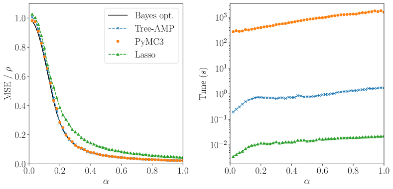
Figure 5: Benchmark on a sparse linear regression task: rescaled MSE as a function of $\alpha=M/N$. The MSE achieved by Tree-AMP (blue) is compared to the Bayes-optimal MMSE (black), Hamiltonian Monte-Carlo (orange) from PyMC3 (with $n_{\rm s}=1000$ distribution samples and NUTS sampler) and Lasso (green) from Scikit-Learn (with the optimal regularization parameter obtained beforehand by simulation). The above experiments have been performed with parameters $(N,\rho,\Delta)=(1000,0.05,0.01)$ and have been averaged over 100 samples.

We compare the Tree-AMP performance on this inference task to the Bayes optimal theoretical prediction from (Barbier et al., 2019) to two state of the art algorithms for this task: Hamiltonian Monte-Carlo from the PyMC3 package (Salvatier et al., 2016) and Lasso (L1-regularized linear regression) from the Scikit-Learn package (Pedregosa et al., 2011). Note that to perform our experimental benchmark in Figure 5 the Tree-AMP and PyMC3 algorithms had access to the ground-truth parameters $(\rho,\Delta)$ used to generate the observations. In order to make the benchmark as fair as possible, we use the optimal regularization parameter for the Lasso, obtained beforehand by simulation.

We observe in Figure 5 (left) that for this model Tree-AMP is Bayes-optimal and reaches the MMSE, up to finite size fluctuations, just as PyMC3. They naturally both outperform Lasso from Scikit-Learn that never achieves the Bayes-optimal MMSE for the full range of aspect ratio $\alpha$ under investigation. This is expected and unfair to Lasso as the two Bayesian methods have full knowledge of the exact generating distribution in our toy model, but this is rarely the case in real applications.

Whereas the Hamiltonian Monte-Carlo algorithm requires to draw a large number of samples ($n_{\rm s}=10^{3}$) to reach a given threshold of precision, Tree-AMP is an iterative algorithm that converges in a few iterations varying broadly speaking between $[10^{0};10^{2}]$. It leads interestingly to an execution time smaller by two orders of magnitude with respect to PyMC3 as illustrated in Figure 5 (right). Hence the fast convergence and execution time of Tree-AMP is certainly a deep asset over PyMC3, or similar Markov Chain Monte-Carlo packages.

4.2 Depicting Tree-AMP modularity

In order to show the adaptability and modularity of Tree-AMP to handle various inference tasks, we present here different examples where the prior distributions are modified flexibly. In particular, we consider first Gaussian denoising of synthetic data with either sparse discrete Fourier transform (DFT) or sparse gradient, and second the denoising and inpainting of real images drawn from the MNIST data set, using a trained Variational Auto-Encoder (VAE) as a prior.

4.2.1 Sparse DFT/gradient denoising

Let us consider a signal $x\in\mathbb{R}^{N}$ corrupted by a Gaussian noise $\xi\sim\mathcal{N}(0,\Delta)$, that leads to the observation $y\in\mathbb{R}^{N}$ according to

$$y=x+\xi$$ (172)

In contrast to the first section in which we considered the signal $x$ to be sparse, we assume here that the signal is dense but that a linear transformation of the signal is sparse. In other words let us define the variable $z=\Omega x$ that we assume to be sparse, where $\Omega$ denotes a linear operator acting on the signal. The factor graph associated to this model is depicted in Figure 6.

Figure 6: Factor graph for sparse $\Omega$ denoising, where $\Omega$ represents either the DFT or the gradient operator.

As a matter of clarity, we focus on two toy one-dimensional signals:

1. $x\in\mathbb{R}^{N}$ such that $\forall n\in[1:N],x_{n}=\cos(t_{n})+\sin(2t_{n})$, with $t_{n}=2\pi(-1+\frac{2n}{N})$. The signal is sparse in the Fourier basis with only two spikes, that leads us to consider a sparse DFT prior: $\Omega$ is the discrete Fourier transform,

2. $x\in\mathbb{R}^{N}$ such that it is randomly drawn constant by pieces. Its gradient contains a lot of zeros and therefore inference with a sparse gradient prior is appropriate: $\Omega$ is the gradient operator.

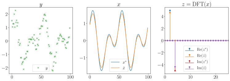
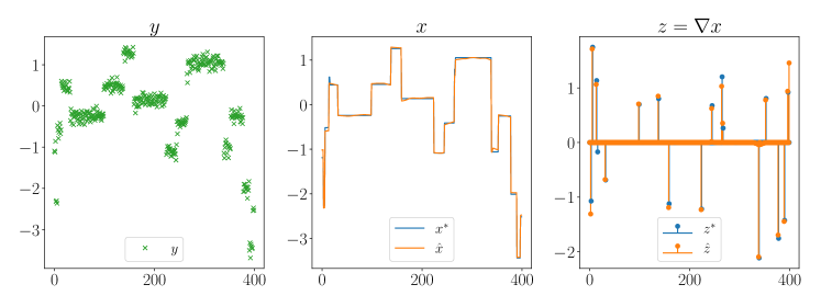
Figure 7: Sparse FFT/gradient denoising: (left) noisy observation $y$, (middle) ground truth signal $x^{*}$ and predicted $\hat{x}$ and (right) ground truth linear transform $z^{*}$ and predicted $\hat{z}$ for (upper) sparse DFT denoising with $(N,\rho,\Delta)=(100,0.02,0.1)$ and (lower) sparse gradient denoising with $(N,\rho,\Delta)=(400,0.04,0.01)$.

After importing the relevant modules, declaring the model in the Tree-AMP package is simple, for instance for the sparse gradient model:

⬇

1# sparse gradient denoising

2model = (

3 GaussianPrior(size=N) @ V(’x’, n_prev=1, n_next=2) @ (

4 GaussianLikelihood(var=Delta, y=y) + (

5 GradientChannel() +

6 GaussBernoulliPrior(rho=rho, size=(1,N))

7 ) @ V(’z’, n_prev=2, n_next=0)

8 )

9).to_model()

For the sparse DFT model, one just needs to replace GradientChannel by DFTChannel. Numerical experiments are shown in Figure 7. The left panel shows the observation $y$, while the middle and right panels illustrate the Tree-AMP reconstruction of the signal $\hat{x}$ and of its linear transform $\hat{z}$ compared to the ground truth $x^{*}$ and $z^{*}$. The Tree-AMP reconstruction approaches closely the ground truth signal and leads to MSE $\sim 10^{-2}/10^{-3}$ for signals $1/2$.

4.2.2 Variational Auto-Encoder on MNIST

Let us consider a signal $x\in\mathbb{R}^{N}$ (with $N=784$) drawn from the MNIST data set. We want to reconstruct the original image from a corrupted observation $y=\varphi(x)\in\mathbb{R}^{N}$, where $\varphi:\mathbb{R}^{N}\to\mathbb{R}^{N}$ represents a noisy channel. In the following the noisy channel represents either a Gaussian additive channel or an inpainting channel, that erases some pixels of the input image.

In order to reconstruct correctly the MNIST image, we investigated the possibility of using a generative prior such as a Variational Auto-Encoder (VAE) along the lines of (Bora et al., 2017; Fletcher et al., 2018). The information theoretical and approximate message passing properties of reconstruction of a low rank or GLM channel, using a dense feed-forward neural network generative prior with $\rm iid$ weights has been studied in particular in (Aubin et al., 2019b, a). The VAE architecture is summarized in Figure 8 and the training procedure on the MNIST data set follows closely the canonical one detailed in (Keras-VAE, ). We considered two common inference tasks: denoising and inpainting.

Figure 8: Denoising/inpaiting a MNIST image with a VAE prior. The weights $W_{1},W_{2}$ and biases $b_{1},b_{2}$ were learned beforehand on the MNIST data set.

Denoising:

In that case, the corrupted channel $\varphi_{\rm den,\Delta}$ adds a Gaussian noise and corresponds to the noisy channel

$$\varphi_{\rm den,\Delta}(x)=x+\xi\quad\textrm{with}\quad\xi\sim\mathcal{N}(0,\Delta)\,.$$

Inpaiting:

The corrupted channel erases a few pixels of the input image and corresponds formally to

$$\varphi_{\rm inp,I_{\alpha}}(x)=\begin{cases}0\textrm{ if }i\in\rm{I}_{\alpha}\,,\\ x_{i}\textrm{ otherwise}\,.\end{cases}$$

where $\rm{I}_{\alpha}$ denotes the set of erased indexes of size $\left\lfloor\alpha N\right\rfloor$ for some $\alpha\in[0;1]$. As an illustration, we consider two different manners of generating the erased interval $I_{\alpha}$:

1. A central horizontal band of width $\lfloor\alpha N\rfloor$: $\rm{I}_{\alpha}^{\rm band}=[\lfloor\frac{N}{2}(1-\alpha)\rfloor;\lfloor\frac{N}{2}(1+\alpha)\rfloor]$

2. Indices drawn uniformly at random $\lfloor\alpha N\rfloor$ : $\rm{I}_{\alpha}^{\rm uni}\sim U([1,N];\lfloor\alpha N\rfloor)$

Solving these inference tasks in Tree-AMP is straightforward: first declare the model Figure 8 and then run Expectation Propagation as exemplified in Section 4.1 for the sparse regression case. A few MNIST samples $x^{*}$ compared to the noisy observations $y$ and Tree-AMP reconstructions $\hat{x}$ are presented in Figure 9, that suggest that Tree-AMP is able to use the trained VAE prior information to either denoise very noisy observations or reconstruct missing pixels.

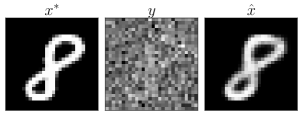
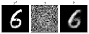
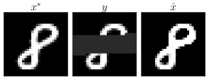
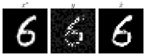
Figure 9: Illustration of the Tree-AMP prediction $\hat{x}$ using a VAE prior from observation $y=\varphi(x^{*})$ with $x^{*}$ a MNIST sample. (left) Denoising $\varphi=\varphi_{\rm den,\Delta}$ with $\Delta=4$. (right-upper) Band-inpainting $\varphi_{\rm inp,I_{\alpha}^{\rm band}}$ with $\alpha=0.3$ (right-lower) Uniform-inpainting $\varphi_{\rm inp,I_{\alpha}^{\rm uni}}$ with $\alpha=0.5$.

4.3 Theoretical prediction of performance

Previous sections were devoted to applications of the Expectation Propagation (EP) Algorithm 2 implemented in Tree-AMP. Moreover the state evolution (SE) Algorithm 5 has also been implemented in the package. This two-in-one package makes it easier to obtain performances of the EP algorithm on finite size instances as well as the infinite size limit behavior predicted by the state evolution.

We illustrate this on two generalized linear models: compressed sensing and sparse phase retrieval, whose common factor graph is represented in Figure 10. Briefly, we consider a sparse $x\in\mathbb{R}^{N}$ $\rm iid$ drawn from a Gauss-Bernoulli distribution $\mathcal{N}_{\rho}$. We observe $y\in\mathbb{R}^{M}=\varphi(Ax)$ with $A\in\mathbb{R}^{M\times N}$ a Gaussian $\rm iid$ matrix, and the noiseless channel is $\varphi(x)=x$ in the compressed sensing case and $\varphi(x)=|x|$ in the phase retrieval one.

Figure 10: Graphical model representing the compressed sensing ($\varphi(x)=x)$) and phase retrieval ($\varphi(x)=|x|)$). We denote $\alpha=M/N$ the aspect ratio of the sensing matrix $A$.

Getting the MSE predicted by state evolution is straightforward in the Tree-AMP package. After importing the relevant modules, one just needs to declare the model and run the SE algorithm. For instance for the sparse phase retrieval model:

⬇

1# declare sparse phase retrieval model

2model = (

3 GaussBernoulliPrior(rho=rho, size=N) @ V(’x’) @

4 LinearChannel(A) @ V(’z’) @

5 AbsLikelihood(y=y)

6).to_model()

7# run SE

8from tramp.algos import StateEvolution

9se = StateEvolution(model)

10se.iterate(max_iter=200)

In Figure 11, we compare the MSE theoretically predicted by state evolution and the MSE obtained on high-dimensional ($N=2000$) instances of EP. Notably up to finite size effects, the MSE averaged over 25 instances of EP match perfectly the MSE predicted by SE. Also the MSE is equal to the Bayes optimal MMSE proven in (Barbier et al., 2019), except for a region of $\alpha$ values known as the hard phase. In that phase, there is a significant gap between the MMSE that is information-theoretically achievable and the MSE actually achieved by EP.

Note that the MMSE is also a state evolution fixed point (Section 3.4) and can thus be obtained by initializing the SE Algorithm 5 in the right basin of attraction. For the two models discussed here, we found that initializing the incoming prior message $\hat{m}_{x\rightarrow\mathcal{N}_{\rho}}\gg 1$ was sufficient to converge towards the MMSE and obtain the Bayes optimal curve.

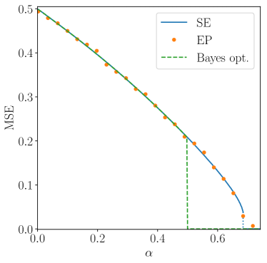
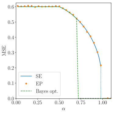
Figure 11: MSE as a function of $\alpha=M/N$ for (left) Compressed sensing ($\rho=0.5$), (right) Sparse phase retrieval ($\rho=0.6$).

5 Discussion

Modularity

The Tree-AMP package aims to solve compositional inference tasks, which can be broken down into local inference problems. As long as the underlying factor graph is tree-structured, the global inference task can be solved by message passing using Algorithm 2, which is just a particular instance of EP. Note that Algorithm 2 is generic, meaning that it can be implemented independently of the probabilistic graphical model under consideration. The main strength of the presented approach is therefore its modularity. In the Tree-AMP package, each module corresponds to a local inference problem given by a factor and associated beliefs on its variables. As long as the module is implemented (which means computing the log-partition $A_{f}[\lambda_{f}]$ and the moment function $\mu_{f}[\lambda_{f}]$), it can be composed at will with other modules to solve complex inference tasks. Several popular machine learning tasks can be reformulated that way as illustrated in Figure 1. We hope that the Tree-AMP package offers a unifying framework to run these models, as well as study them theoretically using the state evolution and free entropy formalism. Below, we review some shortcomings of the Tree-AMP package and possible ways to overcome them.

Hyper-parameter learning

In principle, it should be straightforward to learn hyper-parameters. As usually done in hierarchical Bayesian modelling, one simply needs to add the hyper-parameters as scalar variables in the graphical model with associated hyper priors. In term of the Tree-AMP package, one would simply need to implement the corresponding module (where the set of variables of the factor now includes the hyper-parameters to learn). In the typical use case, where the signals are high dimensional but the hyper-parameters are just scalars, Algorithm 2 will likely be equivalent to the Expectation-Maximization (Dempster et al., 1977) learning of hyper-parameters, as usually done in AMP algorithms (Krzakala et al., 2012).

Generic belief

While the message passing Algorithm 2 is formulated for any kind of beliefs, the current Tree-AMP implementation only supports isotropic Gaussian beliefs. However we could consider more generic beliefs to deal with more complicated types of variable, such as Gaussian process beliefs (Rasmussen and Williams, 2006) for functions or harmonic exponential family beliefs (Cohen and Welling, 2015) for elements of compact groups. Maybe one can recover algorithms similar to (Opper and Winther, 2000) for Gaussian process classification or (Perry et al., 2018) for synchronisation problems over compact groups, and reformulate them in a more modular way. Even if we restrict ourselves to Gaussian beliefs, it may be beneficial to go beyond the isotropic case and consider diagonal or full covariance beliefs (Opper and Winther, 2005a), or any kind of prescribed covariance structure. As exemplified in the committee machine keeping a covariance between experts leads to a more accurate algorithm (Aubin et al., 2018).

Beyond trees

By design, the Tree-AMP package can only handle tree-structured factor graphs. To overcome this fundamental limitation and extend to generic factor graphs, one could use the Kikuchi free energy (Yedidia and Freeman, 2001) in place of the Bethe free energy as a starting point. Similar to the Bethe free energy which is exact for tree-structured factor graphs, the Kikuchi free energy will be exact if the graphical model admits a hyper-tree factorization (Wainwright and Jordan, 2008). The minimization of the Kikuchi free energy under weak consistency constraints (Zoeter and Heskes, 2005) could be used to implement a generalization of Algorithm 2, however the message passing will be more challenging than in the tree case. An equivalent of Proposition 2 will likely hold, where the tree decomposition Eqs (39)-(40) found for the EC Gibbs and EP free energies will be replaced by the hyper-tree factorization.

Convergence

The message passing Algorithm 2, like other EP algorithms, is not guaranteed to converge. This is a major drawback, and indeed on some instances the naive application of Algorithm 2 will diverge. Double loop algorithms like (Heskes and Zoeter, 2002) will ensure convergence, but are unfortunately very slow. In practice, damping the updates is often sufficient to converge towards a fixed point. In the Tree-AMP package the amount of damping has to be chosen by the user. It will be therefore interesting to generalize the adaptive damping scheme (Vila et al., 2015) in order to tune this damping automatically.

Proofs

In Section 3, we heuristically derive the free entropy using weak consistency on the overlaps and conjecture the corresponding state evolution, but did not provide any rigorous proof. We nonetheless recovered earlier derivations of these results for specific models. For instance in the multi-layer model with orthogonally invariant weight matrices, the state evolution was rigorously proven by Fletcher et al. (2018) while the free potential was heuristically derived using the replica method (Gabrié et al., 2018). When the weight matrices are Gaussian, the replica free entropy can further be shown to be rigorous (Reeves and Pfister, 2016; Barbier et al., 2019). One extension of our work would be to generalize existing proofs to arbitrary tree-structured models. In particular it would be beneficial to determine under which conditions the overlaps are the relevant order parameters and if our weak consistency derivation is indeed asymptotically exact.

Acknowledgments

This work is supported by the ERC under the European Union’s Horizon 2020 Research and Innovation Program 714608-SMiLe, as well as by the French Agence Nationale de la Recherche under grant ANR-17-CE23-0023-01 PAIL. Additional funding is acknowledged by AB from ‘Chaire de recherche sur les modèles et sciences des données’, Fondation CFM pour la Recherche-ENS.

Appendix A Proof of Proposition 2

A.1 Minimization of $G[\mu_{V}]$

Let’s first minimize the Bethe free energy at fixed moments $\mu_{V}=(\mu_{i})_{i\in V}$:

$$F_{\mu_{V}}=\min_{(\tilde{p}_{F},\tilde{p}_{V})\in\mathcal{M}_{\mu_{V}}}\mathcal{F}_{\text{Bethe}}[\tilde{p}_{F},\tilde{p}_{V}]$$ (173)

where $\mathcal{M}_{\mu_{V}}$ is the set of factor and variable marginals at fixed moment:

$$\mathcal{M}_{\mu_{V}}=\left\{(\tilde{p}_{F},\tilde{p}_{V})\quad:\quad\forall(i,k)\in E,\quad\mathbb{E}_{\tilde{p}_{i}}\phi_{i}(x_{i})=\mathbb{E}_{\tilde{p}_{k}}\phi_{i}(x_{i})=\mu_{i}\right\}.$$ (174)

The solution will be a stationary point of the Lagrangian

$$\begin{split}&\mathcal{L}[\tilde{p}_{F},\tilde{p}_{V},\lambda_{F},\lambda_{V}]=\mathcal{F}_{\text{Bethe}}[\tilde{p}_{F},\tilde{p}_{V}]\\ &+\sum_{k\in F}\sum_{i\in\partial k}\langle\lambda_{i\to k},\mu_{i}-\mathbb{E}_{\tilde{p}_{k}}\phi_{i}(x_{i})\rangle+\sum_{i\in V}(1-n_{i})\langle\lambda_{i},\mu_{i}-\mathbb{E}_{\tilde{p}_{i}}\phi_{i}(x_{i})\rangle\end{split}$$ (175)

with Lagrange multipliers $\lambda_{i\to k}$ and $\lambda_{i}$ associated to the moment constraint $\mathbb{E}_{\tilde{p}_{k}}\phi_{i}(x_{i})=\mu_{i}$ and $\mathbb{E}_{\tilde{p}_{i}}\phi_{i}(x_{i})=\mu_{i}$. Then $0=\delta_{\tilde{p}_{i}}\mathcal{L}=\delta_{\tilde{p}_{k}}\mathcal{L}=\partial_{\lambda_{i\to k}}\mathcal{L}=\partial_{\lambda_{i}}\mathcal{L}$ leads to the solution:

$$\tilde{p}_{k}(x_{k})=p_{k}(x_{k}\mid\lambda_{k})=f(x_{k};y_{k})\,e^{\langle\lambda_{k},\phi_{k}(x_{k})\rangle-A_{k}[\lambda_{k}]},$$ (176)

$$\tilde{p}_{i}(x_{i})=p_{i}(x_{i}\mid\lambda_{i})=e^{\langle\lambda_{i},\phi_{i}(x_{i})\rangle-A_{i}[\lambda_{i}]},$$ (177)

$$\mu_{i}=\mu_{i}[\lambda_{i}]=\mu_{i}^{k}[\lambda_{k}].$$ (178)

Besides the minimal $F_{\mu_{V}}$ is equal to:

$$F_{\mu_{V}} =\sum_{k\in F}F_{k}[\tilde{p}_{k}]+\sum_{i\in V}(1-n_{i})F_{i}[\tilde{p}_{i}]$$

$$=\sum_{k\in F}\textrm{KL}[\tilde{p}_{k}\|f_{k}]+\sum_{i\in V}(1-n_{i})(-\mathrm{H}[\tilde{p}_{i}])$$

$$=\sum_{k\in F}\textrm{KL}[p_{k}(x_{k}\mid\lambda_{k})\|f_{k}(x_{k};y_{k})]+\sum_{i\in V}(1-n_{i})(-\mathrm{H}[p_{i}(x_{i}|\lambda_{i})])$$

$$=\sum_{k\in F}G[\mu_{k}]+\sum_{i\in V}(1-n_{i})G_{i}[\mu_{i}]$$

$$=G[\mu_{V}],$$

due to the definition Eq. (10) of the Bethe free energy, the fact that the solutions $\tilde{p}_{k}$ and $\tilde{p}_{i}$ belong to the exponential families Eqs (176)-(177), and the definitions Eqs (26)-(27) of $G_{k}$ and $G_{i}$. But then the relaxed Bethe variational problem Eq. (13) can be written as:

$$F_{\phi}(\mathbf{y})=\min_{\mu_{V}}\min_{(\tilde{p}_{F},\tilde{p}_{V})\in\mathcal{M}_{\mu_{V}}}\mathcal{F}_{\text{Bethe}}[\tilde{p}_{F},\tilde{p}_{V}]=\min_{\mu_{V}}F_{\mu_{V}}=\min_{\mu_{V}}G[\mu_{V}].$$ (179)

Besides minimizing $G[\mu_{V}]$ leads to:

$$0=\partial_{\mu_{i}}G[\mu_{V}]=\sum_{k\in\partial i}\lambda_{i\to k}+(1-n_{i})\lambda_{i}$$ (180)

which is the natural parameter constraint. The solution is therefore the same as the EP fixed point Eq. (46).

A.2 Stationary point of $A[\lambda_{V},\lambda_{F}]$

Using the duality (Section 2.4) between natural parameters and moments:

$$\min_{\mu_{V}}G[\mu_{V}] =\min_{\mu_{V}}\sum_{k\in F}G_{k}[\mu_{k}]+\sum_{i\in V}(1-n_{i})G_{i}[\mu_{i}]$$

$$=\min_{\mu_{V}}\sum_{k\in F}\max_{\lambda_{k}}\left\{\langle\lambda_{k},\mu_{k}\rangle-A_{k}[\lambda_{k}]\right\}+\sum_{i\in V}\underbrace{(1-n_{i})}_{\leq 0}\max_{\lambda_{i}}\left\{\langle\lambda_{i},\mu_{i}\rangle-A_{i}[\lambda_{i}]\right\}$$

$$=\min_{\mu_{V}}\min_{\lambda_{V}}\max_{\lambda_{F}}-\sum_{k\in F}A_{k}[\lambda_{k}]-\sum_{i\in V}(1-n_{i})A_{i}[\lambda_{i}]$$

$$+\sum_{i\in V}\langle\sum_{k\in\partial i}\lambda_{i\to k}+(1-n_{i})\lambda_{i},\;\mu_{i}\rangle$$

$$=\min_{\lambda_{V}}\max_{\lambda_{F}}-A[\lambda_{V},\lambda_{F}]\quad\text{s.t}\quad\forall i\in V:(n_{i}-1)\lambda_{i}=\sum_{k\in\partial i}\lambda_{i\to k}.$$ (181)

As a consistency check, let’s directly derive the solution to Eq. (181). Consider the Lagrangian

$$\mathcal{L}[\lambda_{V},\lambda_{F},\mu_{V}]=A[\lambda_{V},\lambda_{F}]+\sum_{i\in V}\langle(n_{i}-1)\lambda_{i}-\sum_{k\in\partial i}\lambda_{i\to k},\;\mu_{i}\rangle$$ (182)

with Lagrangian multiplier $\mu_{i}$ associated to the constraint $(n_{i}-1)\lambda_{i}=\sum_{k\in\partial i}\lambda_{i\to k}$. At a stationary point:

$$\partial_{\mu_{i}}\mathcal{L}=0 \implies(n_{i}-1)\lambda_{i}=\sum_{k\in\partial i}\lambda_{i\to k}$$ (183)

$$\partial_{\lambda_{i\to k}}\mathcal{L}=0 \implies\mu_{i}=\mu_{i}^{k}[\lambda_{k}]$$ (184)

$$\partial_{\lambda_{i}}\mathcal{L}=0 \implies\mu_{i}=\mu_{i}[\lambda_{i}]$$ (185)

which is exactly the same as the EP fixed point Eq. (46). Furthermore the Lagrangian multiplier is the posterior moment $\mu_{i}$.

A.3 Stationary point of $A[\lambda_{E}]$

Finally, the optimization under constraint of $A[\lambda_{V},\lambda_{F}]$ is equivalent to finding a stationary point of $A[\lambda_{E}]$ without any constraint. Indeed:

$$\partial_{\lambda_{k\to i}}A[\lambda_{E}]=0\implies\mu_{i}[\lambda_{i}^{k}]=\mu_{i}[\lambda_{i}]\implies\lambda_{i}^{k}=\lambda_{i}$$ (186)

$$\partial_{\lambda_{i\to k}}A[\lambda_{E}]=0\implies\mu_{i}^{k}[\lambda_{k}]=\mu_{i}[\lambda_{i}^{k}]$$ (187)

which implies the natural parameter constraint

$$\sum_{k\in\partial i}\lambda_{i\to k}=\sum_{k\in\partial i}(\lambda_{i}^{k}-\lambda_{k\to i})=n_{i}\lambda_{i}-\lambda_{i}=(n_{i}-1)\lambda_{i}$$ (188)

and the moment matching $\mu_{i}^{k}[\lambda_{k}]=\mu_{i}[\lambda_{i}]$ defining the EP fixed point Eq. (46).

Appendix B MAP estimation

To yield the maximum at posterior (MAP) estimate, we follow the derivation given in Appendix A.1 of (Manoel et al., 2018) in the context of the TV-VAMP algorithm and generalize it to tree-structured models. As usual in statistical physics literature (Mézard and Montanari, 2009) we introduce an inverse temperature $\beta$ and consider the distribution:

$$p^{(\beta)}(\mathbf{x}\mid\mathbf{y})=\frac{1}{Z^{(\beta)}(\mathbf{y})}\prod_{k\in F}f_{k}(x_{k};y_{k})^{\beta}=\frac{1}{Z^{(\beta)}(\mathbf{y})}e^{-\beta\sum_{k\in F}E_{k}(x_{k};y_{k})}$$ (189)

and take the limit $\beta\to\infty$ to make the distribution concentrate around its mode. Indeed by the Laplace method:

$$F^{(\beta)}(\mathbf{y})=-\frac{1}{\beta}\ln Z^{(\beta)}(\mathbf{y})=-\frac{1}{\beta}\int d\mathbf{x}e^{-\beta E(\mathbf{y})}\xrightarrow{\beta\to\infty}F^{(\infty)}(\mathbf{y})=\min_{\mathbf{x}}E(\mathbf{x},\mathbf{y})$$ (190)

where $E$ is the total energy of the system:

$$E(\mathbf{x},\mathbf{y})=\sum_{k\in F}E_{k}(x_{k};y_{k}).$$ (191)

The inference problem becomes an energy minimization problem, the minimizer $\mathbf{x}^{*}=\operatorname*{arg\,min}_{\mathbf{x}}E(\mathbf{x},\mathbf{y})$ is the MAP estimate and called the ground state in statistical physics (Mézard and Montanari, 2009).

Limit of the weak consistency derivation

At fixed $\beta$, the weak consistency approximation Proposition 2, here expressed for isotopic Gaussian beliefs, gives:

$$F_{\phi}^{(\beta)}(\mathbf{y})=\min_{r_{V}^{(\beta)},\tau_{V}^{(\beta)}}G^{(\beta)}[r_{V}^{(\beta)},\tau_{V}^{(\beta)}]=\min\operatorname*{extr}_{a_{E}^{(\beta)},b_{E}^{(\beta)}}-A^{(\beta)}[a_{E}^{(\beta)}.b_{E}^{(\beta)}]$$ (192)

The limiting behavior can easily be found by scaling the natural parameters $a^{(\beta)}=\beta a$ and $b^{(\beta)}=\beta b$. By the Laplace method, the factor log-partitions are given by:

$$A_{k}^{(\beta)}[a_{k}^{(\beta)},b_{k}^{(\beta)}] =\frac{1}{\beta}\ln\int dx_{k}\,f_{k}(x_{k};y_{k})^{\beta}e^{-\frac{a_{k}^{(\beta)}}{2}\|x_{k}\|^{2}+b_{k}^{(\beta)\intercal}x_{k}}$$

$$=\frac{1}{\beta}\ln\int dx_{k}\,e^{-\beta\{E_{k}(x_{k};y_{k})+\frac{a_{k}}{2}\|x_{k}\|^{2}-b_{k}^{\intercal}x_{k}\}}$$

$$\xrightarrow{\beta\to\infty}A_{k}^{(\infty)}[a_{k},b_{k}]=-\min_{x_{k}}E_{k}(x_{k};y_{k},a_{k},b_{k})$$

where we introduce the tilted energy function:

$$E_{k}(x_{k};y_{k},a_{k},b_{k})=E_{k}(x_{k};y_{k})+\frac{a_{k}}{2}\|x_{k}\|^{2}-b_{k}^{\intercal}x_{k}.$$ (193)

The limiting factor log-partition is thus given by:

$$A_{k}^{(\infty)}[a_{k},b_{k}]=-E_{k}(x_{k}^{*};y_{k},a_{k},b_{k})\quad\text{with}\quad x_{k}^{*}=\operatorname*{arg\,min}_{x_{k}}E_{k}(x_{k}^{*};y_{k},a_{k},b_{k})$$ (194)

which can be alternatively expressed as:

$$A_{k}^{(\infty)}[a_{k},b_{k}]=\frac{\|b_{k}\|^{2}}{2a_{k}}-\mathcal{M}_{\tfrac{1}{a_{k}}E_{k}(.;y_{k})}\left(\frac{b_{k}}{a_{k}}\right),\quad x_{k}^{*}=\mathrm{prox}_{\tfrac{1}{a_{k}}E_{k}(.;y_{k})}\left(\frac{b_{k}}{a_{k}}\right)$$ (195)

using the Moreau envelop $\mathcal{M}_{g}(y)=\min_{x}\{g(x)+\tfrac{1}{2}\|x-y\|^{2}\}$ and proximal operator $\mathrm{prox}_{g}(y)=\operatorname*{arg\,min}_{x}\{g(x)+\tfrac{1}{2}\|x-y\|^{2}\}$. The moment / natural parameter duality becomes:

$$r_{i}^{k(\beta)}[a_{k}^{(\beta)},b_{k}^{(\beta)}] =\partial_{b_{i\to k}^{(\beta)}}\beta A_{k}^{(\beta)}[a_{k}^{(\beta)},b_{k}^{(\beta)}]\quad\xrightarrow{\beta\to\infty} r_{i}^{k(\infty)}[a_{k},b_{k}] =\partial_{b_{i\to k}}A_{k}^{(\infty)}[a_{k},b_{k}]$$

$$-\frac{N_{i}}{2}\tau_{i}^{k(\beta)}[a_{k}^{(\beta)},b_{k}^{(\beta)}] =\partial_{a_{i\to k}^{(\beta)}}\beta A_{k}^{(\beta)}[a_{k}^{(\beta)},b_{k}^{(\beta)}]\quad\xrightarrow{\beta\to\infty} -\frac{N_{i}}{2}\tau_{i}^{k(\infty)}[a_{k},b_{k}] =\partial_{a_{i\to k}}A_{k}^{(\beta)}[a_{k},b_{k}]$$

As the precisions are scaled as $a^{(\beta)}=\beta a$, the variances must be scaled as $\beta v^{(\beta)}=v^{(\infty)}$ and:

$$\beta v_{i}^{k(\beta)}[a_{k}^{(\beta)},b_{k}^{(\beta)}]=\beta\langle\partial^{2}_{b_{i\to k}^{(\beta)}}\beta A_{k}^{(\beta)}[a_{k}^{(\beta)},b_{k}^{(\beta)}]\rangle\quad\xrightarrow{\beta\to\infty}\quad v_{i}^{k\infty}[a_{k},b_{k}]=\langle\partial^{2}_{b_{i\to k}}A_{k}^{(\infty)}[a_{k},b_{k}]\rangle.$$

where $\langle\cdot\rangle$ denotes the average over components of $x_{i}$. From Eq. (194), we then get the posterior mean and second moment:

$$r_{i}^{k(\infty)}[a_{k},b_{k}]=\partial_{b_{i\to k}}A_{k}^{(\infty)}[a_{k},b_{k}]=x_{i}^{k*},\quad\tau_{i}^{k(\infty)}[a_{k},b_{k}]=-\frac{2}{N_{i}}\partial_{a_{i\to k}}A_{k}^{(\infty)}[a_{k},b_{k}]=\frac{\|x_{i}^{k*}\|^{2}}{N_{i}}$$

in agreement with the concentration at the mode. Note that in the zero temperature limit the second-moment is the self-overlap $\tau_{i}^{(\infty)}=q_{i}^{(\infty)}=\frac{\|r_{i}^{(\infty)}\|^{2}}{N_{i}}\neq q_{i}^{(\infty)}+v_{i}^{(\infty)}$. Indeed $\beta v_{i}^{(\beta)}\xrightarrow{\beta\to\infty}v_{i}^{(\infty)}$ is the scaled variance, the actual variance $v_{i}^{(\beta)}\xrightarrow{\beta\to\infty}0$. The variable log-partition corresponds to the $E_{i}(x_{i})=0$ special case. The variable log-partition, mean and (scaled) variance are explicitly given by:

$$A_{i}^{(\infty)}[a_{i},b_{i}]=\frac{\|b_{i}\|^{2}}{2a_{i}},\quad r_{i}^{(\infty)}[a_{i},b_{i}]=\partial_{b_{i}}A_{i}^{(\infty)}=\frac{b_{i}}{a_{i}},\quad v_{i}^{(\infty)}[a_{i},b_{i}]=\langle\partial^{2}_{b_{i}}A_{i}^{(\infty)}\rangle=\frac{1}{a_{i}}.$$ (196)

Limit of the EP algorithm

Let us denote $\text{EP}^{(\beta)}$ the instance of the EP Algorithm 2 running with $a^{(\beta)},b^{(\beta)}$ and $r^{(\beta)},v^{(\beta)}$, which can be used to search a stationary point of $A^{(\beta)}[a_{E}^{(\beta)},b_{E}^{(\beta)}]$. Then we have the well defined limit $\text{EP}^{(\beta)}\xrightarrow{\beta\to\infty}\text{EP}^{(\infty)}$ where $\text{EP}^{(\infty)}$ is the instance of the EP Algorithm 2 running with $a,b$ and $r^{(\infty)},v^{(\infty)}$, which can be used to search a stationary point of $A^{(\infty)}[a_{E},b_{E}]$. At an EP fixed point we will have

$$x_{i}^{*}=r_{i}=r_{i}^{k},\quad v_{i}=v_{i}^{k},\quad(n_{i}-1)a_{i}=\sum_{k\in\partial i}a_{i\to k},\quad(n_{i}-1)b_{i}=\sum_{k\in\partial i}b_{i\to k},$$ (197)

and therefore:

$$-A^{(\infty)}[a_{E},b_{E}] =-\sum_{k}A_{k}^{(\infty)}[a_{k},b_{k}]-\sum_{i\in V}(1-n_{i})A_{i}^{(\infty)}[a_{i},b_{i}]$$

$$=\sum_{k}E_{k}(x_{k}^{*};y_{k},a_{k},b_{k})+\sum_{i\in V}(1-n_{i})E_{i}(x_{i}^{*};a_{i},b_{i})$$

$$=\sum_{k}E_{k}(x_{k}^{*};y_{k})$$

$$+\sum_{i\in V}-\frac{\|x_{i}^{*}\|^{2}}{2}\underbrace{\left(\sum_{k\in\partial i}a_{i\to k}+(1-n_{i})a_{i}\right)}_{0}+x_{i}^{*\intercal}\underbrace{\left(\sum_{k\in\partial i}b_{i\to k}+(1-n_{i})b_{i}\right)}_{0}$$

$$=E(\mathbf{x^{*}},\mathbf{y}).$$

Summary

To recap, the energy minimization / MAP estimation problem can be formulated as:

$$F_{\phi}^{(\infty)}(\mathbf{y})=\min_{\mathbf{x}}E(\mathbf{x},\mathbf{y})=\min\operatorname*{extr}_{a_{E},b_{E}}-A^{(\infty)}[a_{E},b_{E}]$$ (198)

which is the $\beta\to\infty$ limit of Proposition 2. A stationary point of $A^{(\infty)}[a_{E},b_{E}]$ can be searched by the $\text{EP}^{(\infty)}$ Algorithm, which is just Algorithm 2 using the MAP modules:

$$A_{k}^{(\infty)}[a_{k},b_{k}]=\frac{\|b_{k}\|^{2}}{2a_{k}}-\mathcal{M}_{\tfrac{1}{a_{k}}E_{k}(.;y_{k})}\left(\frac{b_{k}}{a_{k}}\right),$$

$$r_{k}^{(\infty)}[a_{k},b_{k}]=\mathrm{prox}_{\tfrac{1}{a_{k}}E_{k}(.;y_{k})}\left(\frac{b_{k}}{a_{k}}\right),\quad v_{k}^{(\infty)}[a_{k},b_{k}]=\langle\partial_{b_{k}}r_{k}^{(\infty)}[a_{k},b_{k}]\rangle,$$ (199)

$$A_{i}^{(\infty)}[a_{i},b_{i}]=\frac{\|b_{i}\|^{2}}{2a_{i}},\quad r_{i}^{(\infty)}=\partial_{b_{i}}A_{i}^{(\infty)}=\frac{b_{i}}{a_{i}},\quad v_{i}^{(\infty)}=\partial^{2}_{b_{i}}A_{i}^{(\infty)}=\frac{1}{a_{i}}.$$ (200)

Appendix C Proof of Proposition 6

C.1 Decomposition of $A(n)$

We recall from Eq. (91) that we can formally decompose the SCGF $A(n)$ as:

$$A(n)=A_{N}^{(n)}-A_{N}^{(0)},\quad A_{N}^{(n)}=\frac{1}{N}\ln Z_{N}^{(n)},\quad A_{N}^{(0)}=\frac{1}{N}\ln Z_{N}^{(0)},$$ (201)

where $Z_{N}^{(0)}$ is the partition function of the teacher generative model:

$$p^{(0)}(\mathbf{x}^{(0)},\mathbf{y})=\frac{1}{Z_{N}^{(0)}}\prod_{k\in F}f_{k}^{(0)}(x_{k}^{(0)};y_{k}),$$ (202)

and $Z_{N}^{(n)}$ is the partition function of the replicated system:

$$p^{(n)}(\{\mathbf{x}^{(a)}\}_{a=0}^{n},\mathbf{y})=\frac{1}{Z_{N}^{(n)}}\prod_{k\in F}\left\{f_{k}^{(0)}(x_{k}^{(0)};y_{k})\prod_{a=1}^{n}f_{k}(x_{k}^{(a)};y_{k})\right\}$$ (203)

where $x^{(a)}$ for $a=1\cdots n$ denote the $n$ replicas and $x^{(0)}$ the ground truth. Now the key observation is that both $Z_{N}^{(0)}$ and $Z_{N}^{(n)}$ are partition functions associated to a tree-structured model (and this is actually the same tree). In that case we know that the log-partition can be obtained exactly from the Bethe variational problem which is unfortunately intractable. However following Heskes et al. (2005) we can solve the relaxed Bethe variational problem by enforcing weak consistency (moment matching) instead of the full consistency of the marginals, as reviewed in Section 2 for the derivation of the EP algorithm.

We must nonetheless specify for which sufficient statistics we want to enforce moment-matching, which in that setting we interpret as identifying the relevant order parameters for the thermodynamic limit. In the following, to make the connection with previously derived replica formulas, we will assume that the relevant order parameters are the overlaps:

$$\phi(\mathbf{x})=\left(\frac{x_{i}^{(a)}\cdot x_{i}^{(b)}}{N_{i}}\right)_{i\in V,0\leq a\leq b\leq n}$$ (204)

In some settings other order parameters could be relevant, fortunately the following derivation could be easily extended to these cases.

C.2 Weak consistency derivation of $A_{N}^{(n)}$

Solving the relaxed Bethe variational problem applied to the log-partition $A_{N}^{(n)}=\frac{1}{N}\ln Z_{N}^{(n)}$, using the overlaps Eq. (204) as sufficient statistics, leads to:

$$-A_{N}^{(n)}=\min_{Q_{V}}G^{(n)}[Q_{V}]=\min\operatorname*{extr}_{\hat{Q}_{E}}-A^{(n)}[\hat{Q}_{E}].$$ (205)

where the minimizer corresponds to the overlaps:

$$Q_{V}=(Q_{i}^{(ab)})_{i\in V,0\leq a\leq b\leq n},\quad Q_{i}^{(ab)}=\mathbb{E}\frac{x_{i}^{(a)}\cdot x_{i}^{(b)}}{N_{i}}$$ (206)

with corresponding dual natural parameter messages:

$$\hat{Q}_{E}=(\hat{Q}_{i\to k}^{(ab)},\hat{Q}_{k\to i}^{(ab)})_{(i,k)\in E,0\leq a\leq b\leq n}$$ (207)

The potentials satisfy the tree decomposition:

$$G^{(n)}[Q_{V}]=\sum_{k\in F}\alpha_{k}G_{k}^{(n)}[Q_{k}]+\sum_{i\in V}\alpha_{i}(1-n_{i})G_{i}^{(n)}[Q_{i}]\quad\text{with}\quad Q_{k}=(Q_{i})_{i\in\partial k},$$ (208)

$$A^{(n)}[\hat{Q}_{E}]=\sum_{k\in F}\alpha_{k}A_{k}^{(n)}[\hat{Q}_{k}]-\sum_{(i,k)\in E}\alpha_{i}A_{i}^{(n)}[\hat{Q}_{i}^{k}]+\sum_{i\in V}\alpha_{i}A_{i}^{(n)}[\hat{Q}_{i}]$$

$$\text{with}\quad\hat{Q}_{k}=(\hat{Q}_{i\to k})_{i\in\partial k}\quad\hat{Q}_{i}^{k}=\hat{Q}_{i\to k}+\hat{Q}_{k\to i},\quad\hat{Q}_{i}=\sum_{k\in\partial i}\hat{Q}_{k\to i}.$$ (209)

The factor and variable log-partition are given by:

$$A_{k}^{(n)}[\hat{Q}_{k}]$$

$$=\frac{1}{N_{k}}\ln\int dy_{k}dx_{k}^{(0)}f_{k}^{(0)}(x_{k}^{(0)};y_{k})\left[\prod_{a=1}^{n}dx_{k}^{(a)}f_{k}(x_{k}^{(a)};y_{k})\right]e^{\sum_{i\in\partial k}\sum_{0\leq a\leq b\leq n}\hat{Q}_{i\to k}^{(ab)}x_{i}^{(a)}\cdot x_{i}^{(b)}}$$ (210)

$$A_{i}^{(n)}[\hat{Q}_{i}]=\frac{1}{N_{i}}\ln\int dx_{i}^{(0)}\left[\prod_{a=1}^{n}dx_{i}^{(a)}\right]\,e^{\sum_{0\leq a\leq b\leq n}\hat{Q}_{i}^{(ab)}x_{i}^{(a)}\cdot x_{i}^{(b)}}$$ (211)

and their gradients give the dual mapping to the overlaps:

$$\alpha_{i}^{k}Q_{i}^{k(ab)}=\partial_{\hat{Q}_{i\to k}^{(ab)}}A_{k}^{(n)},\quad Q_{i}^{(ab)}=\partial_{\hat{Q}_{i}^{(ab)}}A_{i}^{(n)}.$$ (212)

$G_{k}$ and $G_{i}$ are the corresponding Legendre transforms. Any stationary point of the potentials (not necessarily the global optima) is a fixed point:

$$Q_{i}^{k(ab)}=Q_{i}^{(ab)},\quad\hat{Q}_{i}^{(ab)}=\sum_{k\in\partial i}\hat{Q}_{k\to i}^{(ab)}.$$ (213)

C.3 Weak consistency derivation of $A_{N}^{(0)}$

The weak consistency derivation of $A_{N}^{(0)}$ is given in Proposition 5 and consistently corresponds to the $n=0$ case (ignoring the replicas and only keeping the ground truth) of $A_{N}^{(n)}$. The teacher second moments and dual messages in $A_{N}^{(0)}$ correspond to the $a=b=0$ overlaps and dual messages in $A_{N}^{(n)}$:

$$\tau_{i}^{(0)}=Q_{i}^{(00)}=\mathbb{E}\frac{\|x_{i}^{(0)}\|^{2}}{N_{i}},\quad-\frac{1}{2}\hat{\tau}_{i\to k}^{(0)}=\hat{Q}_{i\to k}^{(00)},\quad-\frac{1}{2}\hat{\tau}_{k\to i}^{(0)}=\hat{Q}_{k\to i}^{(00)}.$$ (214)

C.4 Weak consistency derivation of $A(n)$

Now we can finally express the SCGF $A(n)$ in Eq. (201) by subtracting the weak consistency derivation $A_{N}^{(0)}$ to the weak consistency derivation of $A_{N}^{(n)}$. We assume that the teacher second moments $\tau_{V}^{(0)}=Q_{V}^{(00)}$ are known (Section 3.2) and are now considered as fixed parameters. The SCGF obtained by weak consistency on the overlaps is given by:

$$-A(n)=\min_{Q_{V}^{\ast}}G(n)[Q_{V}^{\ast}]=\min\operatorname*{extr}_{\hat{Q}_{E}^{\ast}}-A(n)[\hat{Q}_{E}^{\ast}].$$ (215)

where the minimizer corresponds to the overlaps (with the $ab=00$ overlap omitted):

$$Q_{V}^{\ast}=(Q_{i}^{(ab)})_{i\in V,0\leq a\leq b\leq n,ab\neq 00},\quad Q_{i}^{(ab)}=\mathbb{E}\frac{x_{i}^{(a)}\cdot x_{i}^{(b)}}{N_{i}}$$ (216)

with corresponding dual natural parameter messages:

$$\hat{Q}_{E}^{\ast}=(\hat{Q}_{i\to k}^{(ab)},\hat{Q}_{k\to i}^{(ab)})_{(i,k)\in E,0\leq a\leq b\leq n,ab\neq 00}$$ (217)

The potentials satisfy the tree decomposition:

$$G(n)[Q_{V}^{\ast}]=\sum_{k\in F}\alpha_{k}G_{k}(n)[Q_{k}^{\ast}]+\sum_{i\in V}\alpha_{i}(1-n_{i})G_{i}(n)[Q_{i}^{\ast}]\quad\text{with}\quad Q_{k}^{\ast}=(Q_{i}^{\ast})_{i\in\partial k},$$ (218)

$$A(n)[\hat{Q}_{E}^{\ast}]=\sum_{k\in F}\alpha_{k}A_{k}(n)[\hat{Q}_{k}^{\ast}]-\sum_{(i,k)\in E}\alpha_{i}A_{i}(n)[\hat{Q}_{i}^{k\ast}]+\sum_{i\in V}\alpha_{i}A_{i}(n)[\hat{Q}_{i}^{\ast}]$$

$$\text{with}\quad\hat{Q}_{k}^{\ast}=(\hat{Q}_{i\to k}^{\ast})_{i\in\partial k}\quad\hat{Q}_{i}^{k\ast}=\hat{Q}_{i\to k}^{\ast}+\hat{Q}_{k\to i}^{\ast},\quad\hat{Q}_{i}^{\ast}=\sum_{k\in\partial i}\hat{Q}_{k\to i}^{\ast}.$$ (219)

The factor and variable log-partition are now given by:

$$A_{k}(n)[\hat{Q}_{k}^{\ast}]=\frac{1}{N_{k}}\ln\int dy_{k}dx_{k}^{(0)}$$

$$p_{k}^{(0)}(x_{k}^{(0)},y_{k}\mid\hat{\tau}_{k}^{(0)})\left[\prod_{a=1}^{n}dx_{k}^{(a)}f_{k}(x_{k}^{(a)};y_{k})\right]e^{\sum_{i\in\partial k}\sum_{0\leq a\leq b\leq n,ab\neq 00}\hat{Q}_{i\to k}^{(ab)}x_{i}^{(a)}\cdot x_{i}^{(b)}}$$ (220)

$$A_{i}(n)[\hat{Q}_{i}^{\ast}]=\frac{1}{N_{i}}\ln\int dx_{i}^{(0)}p_{i}^{(0)}(x_{i}^{(0)}\mid\hat{\tau}_{i}^{(0)})\left[\prod_{a=1}^{n}dx_{i}^{(a)}\right]e^{\sum_{0\leq a\leq b\leq n,ab\neq 00}\hat{Q}_{i}^{(ab)}x_{i}^{(a)}\cdot x_{i}^{(b)}}$$ (221)

and their gradients give the dual mapping to the overlaps:

$$\alpha_{i}^{k}Q_{i}^{k(ab)}=\partial_{\hat{Q}_{i\to k}^{(ab)}}A_{k}^{(n)},\quad Q_{i}^{(ab)}=\partial_{\hat{Q}_{i}^{(ab)}}A_{i}^{(n)}.$$ (222)

$G_{k}$ and $G_{i}$ are the corresponding Legendre transforms. Any stationary point of the potentials (not necessarily the global optima) is a fixed point:

$$Q_{i}^{k(ab)}=Q_{i}^{(ab)},\quad\hat{Q}_{i}^{(ab)}=\sum_{k\in\partial i}\hat{Q}_{k\to i}^{(ab)}.$$ (223)

Proof.

It follows straightforwardly from $\hat{Q}_{k}^{(00)}=-\frac{1}{2}\hat{\tau}_{k}^{(0)}$ and Eq. (107):

$$A_{k}^{(n)}[\hat{Q}_{k}]-A_{k}^{(0)}[\hat{\tau}_{k}^{(0)}]$$

$$=\frac{1}{N_{k}}\ln\int dy_{k}dx_{k}^{(0)}\,\underbrace{\tfrac{1}{Z_{k}^{(0)}[\hat{\tau}_{k}^{(0)}]}f_{k}^{(0)}(x_{k}^{(0)};y_{k})e^{-\frac{1}{2}\sum_{i\in\partial k}\hat{\tau}_{i\to k}^{0}\|x_{i}^{(0)}\|^{2}}}_{p_{k}^{(0)}(x_{k}^{(0)},y_{k}\mid\hat{\tau}_{k}^{(0)})}\left[\prod_{a=1}^{n}dx_{k}^{(a)}f_{k}(x_{k}^{(a)};y_{k})\right]$$

$$e^{\sum_{i\in\partial k}\sum_{0\leq a\leq b\leq n,ab\neq 00}\hat{Q}_{i\to k}^{(ab)}x_{i}^{(a)}\cdot x_{i}^{(b)}}$$

$$=A_{k}(n)[\hat{Q}_{k}^{\ast}]$$

Similarly it follows straightforwardly from $\hat{Q}_{i}^{(00)}=-\frac{1}{2}\hat{\tau}_{i}^{(0)}$ and Eq. (108):

$$A_{i}^{(n)}[\hat{Q}_{i}]-A_{i}^{(0)}[\hat{\tau}_{i}^{(0)}]$$

$$=\frac{1}{N_{i}}\ln\int dx_{i}^{(0)}\underbrace{\tfrac{1}{Z_{i}^{(0)}[\hat{\tau}_{i}^{(0)}]}e^{-\frac{1}{2}\hat{\tau}_{i}^{0}\|x_{i}^{(0)}\|^{2}}}_{p_{i}^{(0)}(x_{i}^{(0)}\mid\hat{\tau}_{i}^{0})}\left[\prod_{a=1}^{n}dx_{i}^{(a)}\right]e^{\sum_{0\leq a\leq b\leq n,ab\neq 00}\hat{Q}_{i}^{(ab)}x_{i}^{(a)}\cdot x_{i}^{(b)}}$$

$$=A_{i}(n)[\hat{Q}_{i}^{\ast}]$$

∎

C.5 Replica symmetric $A(n)$

We take the replica symmetric ansatz (Mézard et al., 1987) for the overlaps $(1\leq a<b\leq n)$:

$$\tau=Q^{(aa)},\;m=Q^{(0a)},\;q=Q^{(ab)},\quad-\frac{1}{2}\hat{\tau}=\hat{Q}^{(aa)},\;\hat{m}=\hat{Q}^{(0a)},\;\hat{q}=\hat{Q}^{(ab)}.$$ (224)

The replica symmetric SCGF $A(n)$ is given by:

$$-A(n)=\min_{m_{V},q_{V},\tau_{V}}G(n)[m_{V},q_{V},\tau_{V}]=\min\operatorname*{extr}_{\hat{m}_{E},\hat{q}_{E},\hat{\tau}_{E}}-A(n)[\hat{m}_{E},\hat{q}_{E},\hat{\tau}_{E}].$$ (225)

The potentials satisfy the tree decomposition:

$$G(n)[m_{V},q_{V},\tau_{V}]=\sum_{k\in F}\alpha_{k}G_{k}(n)[m_{k},q_{k},\tau_{k}]+\sum_{i\in V}\alpha_{i}(1-n_{i})G_{i}(n)[m_{i},q_{i},\tau_{i}]$$

$$\text{with}\quad m_{k}=(m_{i})_{i\in\partial k}\quad(\text{idem }q,\tau),$$ (226)

$$A(n)[\hat{m}_{E},\hat{q}_{E},\hat{\tau}_{E}]$$

$$=\sum_{k\in F}\alpha_{k}A_{k}(n)[\hat{m}_{k},\hat{q}_{k},\hat{\tau}_{k}]-\sum_{(i,k)\in E}\alpha_{i}A_{i}(n)[\hat{m}_{i}^{k},\hat{q}_{i}^{k},\hat{\tau}_{i}^{k}]+\sum_{i\in V}\alpha_{i}A_{i}(n)[\hat{m}_{i},\hat{q}_{i},\hat{\tau}_{i}]$$

$$\text{with}\quad\hat{m}_{k}=(\hat{m}_{i\to k})_{i\in\partial k},\quad\hat{m}_{i}^{k}=\hat{m}_{i\to k}+\hat{m}_{k\to i},\quad\hat{m}_{i}=\sum_{k\in\partial i}\hat{m}_{k\to i}\quad(\text{idem }q,\tau).$$ (227)

The factor and variable log-partition are given by:

$$A_{k}(n)[\hat{m}_{k},\hat{q}_{k},\hat{\tau}_{k}]=\frac{1}{N_{k}}\mathbb{E}_{p_{k}^{(0)}(x_{k}^{(0)},y_{k},b_{k})}e^{N_{k}nA_{k}[a_{k},b_{k};y_{k}]}$$ (228)

$$A_{i}(n)[\hat{m}_{i},\hat{q}_{i},\hat{\tau}_{i}]=\frac{1}{N_{i}}\mathbb{E}_{p_{i}^{(0)}(x_{i}^{(0)},b_{i})}e^{N_{i}nA_{i}[a_{i},b_{i}]}$$ (229)

taken with:

$$p_{k}^{(0)}(x_{k}^{(0)},y_{k},b_{k}) =\mathcal{N}(b_{k}\mid\hat{m}_{k}x_{k}^{(0)},\hat{q}_{k})\;p_{k}^{(0)}(x_{k}^{(0)},y_{k};\hat{\tau}_{k}^{(0)})\quad \text{and}\quad a_{k} =\hat{\tau}_{k}+\hat{q}_{k},$$ (230)

$$p_{i}^{(0)}(x_{i}^{(0)},b_{i}) =\mathcal{N}(b_{i}\mid\hat{m}_{i}x_{i}^{(0)},\hat{q}_{i})\;p_{i}^{(0)}(x_{i}^{(0)};\hat{\tau}_{i}^{(0)})\quad \text{and}\quad a_{i} =\hat{\tau}_{i}+\hat{q}_{i},$$ (231)

and where $A_{k}[a_{k},b_{k};y_{k}]$ and $A_{i}[a_{i},b_{i}]$ are the scaled EP log-partitions:

$$A_{k}[a_{k},b_{k};y_{k}] =\frac{1}{N_{k}}\ln\int dx_{k}\,f(x_{k};y_{k})\,e^{-\frac{1}{2}a_{k}\|x_{k}\|^{2}+b_{k}^{\intercal}x_{k}}$$ (232)

$$A_{i}[a_{i},b_{i}] =\frac{1}{N_{i}}\ln\int dx_{i}\,e^{-\frac{1}{2}a_{i}\|x_{i}\|^{2}+b_{i}^{\intercal}x_{i}}.$$ (233)

We have therefore the following large deviation theory interpretation:

$$A(n) =\text{SCGF of }A_{N}(\mathbf{y})$$ (234)

$$A_{k}(n) =\text{SCGF of }A_{k}[a_{k},b_{k};y_{k}]$$ (235)

$$A_{i}(n) =\text{SCGF of }A_{i}[a_{i},b_{i}]$$ (236)

Proof.

The replica symmetric ansatz gives:

$$\left.\sum_{0\leq a\leq b\leq n,ab\neq 00}\hat{Q}_{i\to k}^{(ab)}x_{i}^{(a)}\cdot x_{i}^{(b)}\right|_{\text{RS}}$$

$$=\hat{m}_{i\to k}x_{i}^{(0)}\cdot\sum_{a=1}^{n}x_{i}^{(a)}+\hat{q}_{i\to k}\sum_{1\leq a<b\leq n}x_{i}^{(a)}\cdot x_{i}^{(b)}-\frac{\hat{\tau}_{i\to k}}{2}\sum_{a=1}^{n}\|x_{i}^{(a)}\|^{2}$$

$$=\hat{m}_{i\to k}x_{i}^{(0)}\cdot\sum_{a=1}^{n}x_{i}^{(a)}+\frac{\hat{q}_{i\to k}}{2}\|\sum_{a=1}^{n}x_{i}^{(a)}\|^{2}-\frac{\hat{\tau}_{i\to k}+\hat{q}_{i\to k}}{2}\sum_{a=1}^{n}\|x_{i}^{(a)}\|^{2}$$

Using the Gaussian identity:

$$e^{\frac{\hat{q}_{i\to k}}{2}\|\sum_{a=1}^{n}x_{i}^{(a)}\|^{2}}=\int_{\mathbb{R}^{N_{i}}}d\xi_{i\to k}\mathcal{N}(\xi_{i\to k})e^{\sqrt{\hat{q}_{i\to k}}\xi_{i\to k}\cdot\sum_{a=1}^{n}x_{i}^{(a)}}$$

we can express the replica symmetric $A_{k}(n)[\hat{Q}_{k}^{\ast}]$ as:

$$\left.A_{k}(n)[\hat{Q}_{k}^{\ast}]\right|_{\text{RS}}$$

$$=\frac{1}{N_{k}}\ln\int dy_{k}dx_{k}^{(0)}p_{k}^{(0)}(x_{k}^{(0)},y_{k}\mid\hat{\tau}_{k}^{(0)})\left[\prod_{i\in\partial k}d\xi_{i\to k}\mathcal{N}(\xi_{i\to k})\right]\left[\prod_{a=1}^{n}dx_{k}^{(a)}f_{k}(x_{k}^{(a)};y_{k})\right]$$

$$\prod_{a=1}^{n}e^{\sum_{i\in\partial k}[\hat{m}_{i\to k}x_{i}^{(0)}+\sqrt{\hat{q}_{i\to k}}\xi_{i\to k}]\cdot x_{i}^{(a)}-\frac{\hat{\tau}_{i\to k}+\hat{q}_{i\to k}}{2}\|x_{i}^{(a)}\|^{2}}$$

$$=\frac{1}{N_{k}}\ln\int dy_{k}dx_{k}^{(0)}p_{k}^{(0)}(x_{k}^{(0)},y_{k}\mid\hat{\tau}_{k}^{(0)})\left[\prod_{i\in\partial k}db_{i\to k}\mathcal{N}(b_{i\to k}\mid\hat{m}_{i\to k}x_{i}^{(0)},\hat{q}_{i\to k})\right]$$

$$\left[\prod_{a=1}^{n}dx_{k}^{(a)}f_{k}(x_{k}^{(a)};y_{k})e^{\sum_{i\in\partial k}-\frac{a_{i\to k}}{2}\|x_{i}^{(a)}\|^{2}+b_{i\to k}\cdot x_{i}^{(a)}}\right]$$

$$\text{with}\quad b_{i\to k}=\hat{m}_{i\to k}x_{i}^{(0)}+\sqrt{\hat{q}_{i\to k}}\xi_{i\to k},\quad a_{i\to k}=\hat{\tau}_{i\to k}+\hat{q}_{i\to k}.$$

The integration over $x_{k}^{(a)}$ gives the EP partition function

$$Z_{k}[a_{k},b_{k};y_{k}]=\int dx_{k}\,f(x_{k};y_{k})\,e^{\sum_{i\in\partial k}-\frac{1}{2}a_{i\to k}\|x_{i}\|^{2}+b_{i\to k}\cdot x_{k}}$$ (237)

therefore

$$\left.A_{k}(n)[\hat{Q}_{k}^{\ast}]\right|_{\text{RS}}$$

$$=\frac{1}{N_{k}}\ln\int dy_{k}dx_{k}^{(0)}db_{k}\mathcal{N}(b_{k}\mid\hat{m}_{k}x_{k}^{(0)},\hat{q}_{k})p_{k}^{(0)}(x_{k}^{(0)},y_{k}\mid\hat{\tau}_{k}^{(0)})\prod_{a=1}^{n}Z_{k}[a_{k},b_{k};y_{k}]$$

$$=\frac{1}{N_{k}}\ln\mathbb{E}_{p_{k}^{(0)}(x_{k}^{(0)},y_{k},b_{k})}Z_{k}[a_{k},b_{k};y_{k}]^{n}$$

$$=\frac{1}{N_{k}}\ln\mathbb{E}_{p_{k}^{(0)}(x_{k}^{(0)},y_{k},b_{k})}e^{N_{k}nA_{k}[a_{k},b_{k};y_{k}]}\quad\text{with}\quad A_{k}[a_{k},b_{k};y_{k}]=\frac{1}{N_{k}}\ln Z_{k}[a_{k},b_{k};y_{k}]$$

$$=A_{k}(n)[\hat{m}_{k},\hat{q}_{k},\hat{\tau}_{k}]$$

The proof is identical for the replica symmetric $A_{i}(n)[\hat{Q}_{i}^{\ast}]$. ∎

C.6 Replica symmetric $\bar{A}$

We recall from Eq. (90) that the ensemble average $\bar{A}$ can be obtained by:

$$\bar{A}=\left.\frac{d}{dn}A(n)\right|_{n=0}$$ (238)

Taking the derivative Eq. (238) of the replica symmetric $A(n)$ we get Proposition 6 with:

$$\left.\frac{d}{dn}A_{k}(n)[\hat{m}_{k},\hat{q}_{k},\hat{\tau_{k}}]\right|_{n=0}=\mathbb{E}_{p_{k}^{(0)}(x_{k}^{(0)},y_{k},b_{k})}A_{k}[a_{k},b_{k};y_{k}]=\bar{A}_{k}[\hat{m}_{k},\hat{q}_{k},\hat{\tau_{k}}]$$

$$\left.\frac{d}{dn}A_{i}(n)[\hat{m}_{i},\hat{q}_{i},\hat{\tau_{i}}]\right|_{n=0}=\mathbb{E}_{p_{i}^{(0)}(x_{i}^{(0)},b_{i})}A_{i}[a_{i},b_{i}]=\bar{A}_{i}[\hat{m}_{i},\hat{q}_{i},\hat{\tau_{i}}]$$

as expected from the large deviation theory interpretation Eqs (235)-(236).

Appendix D Proof of the information theoretic decomposition

We recall that the local teacher generative model Eq. (154) is given by:

$$p_{k}^{(0)}(x_{k}^{(0)},y_{k},b_{k})=\mathcal{N}(b_{k}\mid\hat{m}_{k}x_{k}^{(0)},\hat{q}_{k})\,p_{k}^{(0)}(x_{k}^{(0)},y_{k}\mid\hat{\tau}_{k}^{(0)}),$$

while the local student generative model Eq. (155) is given by:

$$p_{k}(x_{k},y_{k},b_{k})=\mathcal{N}(b_{k}\mid\hat{q}_{k}x_{k},\hat{q}_{k})\,p_{k}(x_{k},y_{k}\mid\hat{\tau}_{k}).$$

Interestingly by rescaling $b_{k}^{(0)}=\frac{\hat{m}_{k}}{\hat{q}_{k}}b_{k}$ the local teacher generative model is equal to the Bayes-optimal setting generative model Eq. (158):

$$p_{k}^{(0)}(x_{k}^{(0)},y_{k},b_{k}^{(0)})=\mathcal{N}(b_{k}^{(0)}\mid\hat{m}_{k}^{(0)}x_{k}^{(0)},\hat{m}_{k}^{(0)})\,p_{k}^{(0)}(x_{k}^{(0)},y_{k}\mid\hat{\tau}_{k}^{(0)})\quad\text{with}\quad\hat{m}_{k}^{(0)}=\frac{\hat{m}_{k}^{2}}{\hat{q}_{k}}.$$

The RS potential Eq. (119) is related to the cross-entropy between the local teacher evidence $p_{k}^{(0)}(y_{k},b_{k})$ and the local student evidence $p_{k}(y_{k},b_{k})$:

$$\bar{A}_{k}[\hat{m}_{k},\hat{q}_{k},\hat{\tau}_{k}]-A_{k}[\hat{\tau}_{k}]$$

$$=-\frac{1}{N_{k}}H[p_{k}^{(0)}(y_{k},b_{k}),p_{k}(y_{k},b_{k})]+\sum_{i\in\partial k}\frac{\alpha_{i}^{k}\hat{m}_{i\to k}^{(0)}\tau_{i}^{(0)}}{2}+\frac{\alpha_{i}^{k}}{2}\ln 2\pi e\hat{q}_{i\to k}.$$ (239)

Similarly, the BO potential Eq. (141) is related to the entropy of the local Bayes-optimal evidence $p_{k}^{(0)}(y_{k},b_{k}^{(0)})$:

$$\bar{A}_{k}^{(0)}[\hat{m}_{k}^{(0)}]-A_{k}^{(0)}[\hat{\tau}_{k}^{(0)}]\\ =-\frac{1}{N_{k}}H[p_{k}^{(0)}(y_{k},b_{k}^{(0)})]+\sum_{i\in\partial k}\frac{\alpha_{i}^{k}\hat{m}_{i\to k}^{(0)}\tau_{i}^{(0)}}{2}+\frac{\alpha_{i}^{k}}{2}\ln 2\pi e\hat{m}_{i\to k}^{(0)}.$$ (240)

Proof.

The local student evidence is equal to:

$$p_{k}(y_{k},b_{k}) =\int dx_{k}p_{k}(x_{k},y_{k},b_{k})=\int dx_{k}p_{k}(x_{k},y_{k}\mid\hat{\tau_{k}})\mathcal{N}(b_{k}\mid\hat{q}_{k}x_{k},\hat{q}_{k})$$

$$=\int dx_{k}f_{k}(x_{k};y_{k})e^{-\frac{1}{2}\hat{\tau}_{k}\|x_{k}\|^{2}-N_{k}A_{k}[\hat{\tau_{k}}]}e^{-\frac{1}{2}\hat{q}_{k}\|x_{k}\|^{2}+b_{k}^{\intercal}x_{k}}\mathcal{N}(b_{k}\mid 0,\hat{q}_{k})$$

$$=\int dx_{k}f_{k}(x_{k};y_{k})e^{-\frac{1}{2}a_{k}\|x_{k}\|^{2}+b_{k}^{\intercal}x_{k}-N_{k}A_{k}[\hat{\tau_{k}}]}\mathcal{N}(b_{k}\mid 0,\hat{q}_{k})\quad\text{with}\quad a_{k}=\hat{\tau}_{k}+\hat{q}_{k}$$

$$=e^{N_{k}A_{k}[a_{k},b_{k};y_{k}]-N_{k}A_{k}[\hat{\tau}_{k}]}\mathcal{N}(b_{k}\mid 0,\hat{q}_{k})$$

Then:

$$\bar{A}_{k}[\hat{m}_{k},\hat{q}_{k},\hat{\tau}_{k}]-A_{k}[\hat{\tau}_{k}]=\mathbb{E}_{p_{k}^{(0)}(x_{k}^{(0)},y_{k},b_{k})}A_{k}[a_{k},b_{k};y_{k}]-A_{k}[\hat{\tau}_{k}]$$

$$=\frac{1}{N_{k}}\mathbb{E}_{p_{k}^{(0)}(x_{k}^{(0)},y_{k},b_{k})}\ln\frac{p_{k}(y_{k},b_{k})}{\mathcal{N}(b_{k}\mid 0,\hat{q}_{k})}$$

$$=-\frac{1}{N_{k}}H[p_{k}^{(0)}(y_{k},b_{k}),p_{k}(y_{k},b_{k})]+\frac{1}{N_{k}}\mathbb{E}_{p_{k}^{(0)}(x_{k}^{(0)},y_{k},b_{k})}\sum_{i\in\partial k}\frac{\|b_{i\to k}\|^{2}}{2\hat{q}_{i\to k}}+\frac{N_{i}}{2}\ln 2\pi\hat{q}_{i\to k}$$

$$=-\frac{1}{N_{k}}H[p_{k}^{(0)}(y_{k},b_{k}),p_{k}(y_{k},b_{k})]+\frac{1}{N_{k}}\sum_{i\in\partial k}\frac{N_{i}(\hat{m}_{i\to k}^{2}\tau_{i}^{(0)}+\hat{q}_{i\to k})}{2\hat{q}_{i\to k}}+\frac{N_{i}}{2}\ln 2\pi\hat{q}_{i\to k}$$

$$=-\frac{1}{N_{k}}H[p_{k}^{(0)}(y_{k},b_{k}),p_{k}(y_{k},b_{k})]+\sum_{i\in\partial k}\frac{\alpha_{i}^{k}\hat{m}_{i\to k}^{(0)}\tau_{i}^{(0)}}{2}+\frac{\alpha_{i}^{k}}{2}\ln 2\pi e\hat{q}_{i\to k}$$

with $\hat{m}_{i\to k}^{(0)}=\frac{\hat{m}_{i\to k}^{2}}{\hat{q}_{i\to k}}$ and $\alpha_{i}^{k}=\frac{N_{i}}{N_{k}}$ which proves Eq. (239). The proof for the BO potential Eq. (240) is identical to the RS case with the simplifications $\hat{m}_{k}^{(0)}=\hat{q}_{k}=\hat{m}_{k}$ and $\hat{\tau}_{k}=\hat{\tau}_{k}^{(0)}$. ∎

From Eq. (239) we recover the decomposition Eq. (160) for the RS potential:

$$\bar{A}_{k}[\hat{m}_{k},\hat{q}_{k},\hat{\tau}_{k}]-A_{k}[\hat{\tau}_{k}]=\bar{A}_{k}^{(0)}[\hat{m}_{k}^{(0)}]-A_{k}^{(0)}[\hat{\tau}_{k}^{(0)}]-\frac{1}{N_{k}}\mathrm{KL}[p_{k}^{(0)}(y_{k},b_{k})\|p_{k}(y_{k},b_{k})]$$

From Eq. (240) we recover the decomposition Eq. (161) for the BO potential:

$$\bar{A}_{k}^{(0)}[\hat{m}_{k}^{(0)}]-A_{k}^{(0)}[\hat{\tau}_{k}^{(0)}]=\sum_{i\in\partial k}\frac{\alpha_{i}^{k}\hat{m}_{i\to k}^{(0)}\tau_{i}^{(0)}}{2}+\frac{1}{N_{k}}H[p_{k}^{(0)}(b_{k}^{(0)}\mid x_{k}^{(0)})]-\frac{1}{N_{k}}H[p_{k}^{(0)}(y_{k},b_{k}^{(0)})].$$

Proof.

The proof for the BO case is straightforward:

$$p_{k}^{(0)}(b_{k}^{(0)}\mid x_{k}^{(0)})=\mathcal{N}(b_{k}^{(0)}\mid\hat{m}_{k}^{(0)}x_{k}^{(0)},\hat{m}_{k}^{(0)})\implies\frac{1}{N_{k}}H[p_{k}^{(0)}(b_{k}^{(0)}\mid x_{k}^{(0)})]=\sum_{i\in\partial k}\frac{\alpha_{i}^{k}}{2}\ln 2\pi e\hat{m}_{i\to k}^{(0)}.$$

In the RS case, due to the rescaling $b_{k}^{(0)}=\frac{\hat{m}_{k}}{\hat{q}_{k}}b_{k}$ we have for the densities:

$$\frac{1}{N_{k}}\ln p_{k}^{(0)}(y_{k},b_{k}^{(0)})=\frac{1}{N_{k}}\ln p_{k}^{(0)}(y_{k},b_{k})+\sum_{i\in\partial k}\alpha_{i}^{k}\ln\frac{\hat{q}_{i\to k}}{\hat{m}_{i\to k}}$$

which gives for the entropies:

$$-\frac{1}{N_{k}}H[p_{k}^{(0)}(y_{k},b_{k}^{(0)})]=-\frac{1}{N_{k}}H[p_{k}^{(0)}(y_{k},b_{k})]+\sum_{i\in\partial k}\alpha_{i}^{k}\ln\frac{\hat{q}_{i\to k}}{\hat{m}_{i\to k}}$$

Then Eq. (240) at $\hat{m}_{k}^{(0)}=\frac{\hat{m}_{k}^{2}}{\hat{q}_{k}}$ can be written:

$$\bar{A}_{k}^{(0)}[\hat{m}_{k}^{(0)}]-A_{k}^{(0)}[\hat{\tau}_{k}^{(0)}]$$

$$=-\frac{1}{N_{k}}H[p_{k}^{(0)}(y_{k},b_{k})]+\sum_{i\in\partial k}\alpha_{i}^{k}\ln\frac{\hat{q}_{i\to k}}{\hat{m}_{i\to k}}+\sum_{i\in\partial k}\frac{\alpha_{i}^{k}\hat{m}_{i\to k}^{(0)}\tau_{i}^{(0)}}{2}+\frac{\alpha_{i}^{k}}{2}\ln 2\pi e\frac{\hat{m}_{i\to k}^{2}}{\hat{q}_{i\to k}}$$

$$=-\frac{1}{N_{k}}H[p_{k}^{(0)}(y_{k},b_{k})]+\sum_{i\in\partial k}\frac{\alpha_{i}^{k}\hat{m}_{i\to k}^{(0)}\tau_{i}^{(0)}}{2}+\frac{\alpha_{i}^{k}}{2}\ln 2\pi e\hat{q}_{i\to k}$$

By using Eq. (239) we finally get:

$$\bar{A}_{k}[\hat{m}_{k},\hat{q}_{k},\hat{\tau}_{k}]-A_{k}[\hat{\tau}_{k}]$$

$$=\bar{A}_{k}^{(0)}[\hat{m}_{k}^{(0)}]-A_{k}^{(0)}[\hat{\tau}_{k}^{(0)}]-\frac{1}{N_{k}}H[p_{k}^{(0)}(y_{k},b_{k}),p_{k}(y_{k},b_{k})]+\frac{1}{N_{k}}H[p_{k}^{(0)}(y_{k},b_{k})]$$

$$=\bar{A}_{k}^{(0)}[\hat{m}_{k}^{(0)}]-A_{k}^{(0)}[\hat{\tau}_{k}^{(0)}]-\frac{1}{N_{k}}\mathrm{KL}[p_{k}^{(0)}(y_{k},b_{k})\|p_{k}(y_{k},b_{k})]$$

∎

Appendix E Tree-AMP modules

E.1 Variable

The Tree-AMP package only implements isotropic Gaussian beliefs, but the variable log-partitions presented here will be useful to derive the factor modules.

E.1.1 General variable

An approximate belief, which we may as well call a variable type, is specified by the base space $X$ as well as the chosen set of sufficient statistics $\phi(x)$. Any variable type defines an exponential family distribution

$$p(x\mid\lambda)=e^{\langle\lambda,\phi(x)\rangle-A[\lambda]}$$ (241)

indexed by the natural parameter $\lambda$. The family can be alternatively indexed by the moments $\mu=\mathbb{E}_{p(x\mid\lambda)}\phi(x)$. The log-partition

$$A[\lambda]=\ln\int_{X}dxe^{\lambda^{\intercal}\phi(x)}$$ (242)

provides the bijective mapping between the natural parameters and the moments:

$$\mu[\lambda]=\partial_{\lambda}A[\lambda].$$ (243)

For all the variable types considered below, we will always have $x\in\phi(x)$ in the set of sufficient statistics. Its associated natural parameter $b\in\lambda$ is thus dual to the mean $r\in\mu$. The mean and variance are given by:

$$r[\lambda]=\partial_{b}A[\lambda],\qquad v[\lambda]=\partial_{b}^{2}A[\lambda],$$ (244)

We list below the log-partition, mean and variance for several variable types, which correspond to well known exponential family distributions.

E.1.2 Isotropic Gaussian variable

For $x\in\mathbb{R}^{N}$, sufficient statistics $\phi(x)=(x,-\frac{1}{2}x^{\intercal}x)$, natural parameters $\lambda=(b,a)$ with $b\in\mathbb{R}^{N}$ and scalar precision $a\in\mathbb{R}$.

$$A[a,b]=\ln\int dx\,e^{-\frac{1}{2}ax^{\intercal}x+b^{\intercal}x}=\frac{\|b\|^{2}}{2a}+\frac{N}{2}\ln\frac{2\pi}{a},$$ (245)

$$r[a,b]=\frac{b}{a},\qquad v[a,b]=\frac{1}{a}\in\mathbb{R}.$$ (246)

The corresponding exponential family is the isotropic multivariate Normal:

$$p(x\mid a,b)=\mathcal{N}(x\mid r,v)\quad\text{with}\quad r=\frac{b}{a},\quad v=\frac{1}{a}.$$ (247)

E.1.3 Diagonal Gaussian variable

For $x\in\mathbb{R}^{N}$, sufficient statistics $\phi(x)=(x,-\frac{1}{2}x^{2})$, natural parameters $\lambda=(b,a)$ with $b\in\mathbb{R}^{N}$ and diagonal precision $a\in\mathbb{R}^{N}$.

$$A[a,b]=\ln\int dx\,e^{-\frac{1}{2}x^{\intercal}ax+b^{\intercal}x}=\sum_{n=1}^{N}\frac{b_{n}^{2}}{2a_{n}}+\frac{1}{2}\ln\frac{2\pi}{a_{n}},$$ (248)

$$r[a,b]=\frac{b}{a},\qquad v[a,b]=\frac{1}{a}\in\mathbb{R}^{N}.$$ (249)

The corresponding exponential family is the diagonal multivariate Normal:

$$p(x\mid a,b)=\mathcal{N}(x\mid r,v)\quad\text{with}\quad r=\frac{b}{a},\quad v=\frac{1}{a}.$$ (250)

E.1.4 Full covariance Gaussian variable

For $x\in\mathbb{R}^{N}$, sufficient statistics $\phi(x)=(x,-\frac{1}{2}xx^{\intercal})$, natural parameters $\lambda=(b,a)$ with $b\in\mathbb{R}^{N}$ and matrix precision $a\in\mathbb{R}^{N\times N}$.

$$A[a,b]=\ln\int dx\,e^{-\frac{1}{2}x^{\intercal}ax+b^{\intercal}x}=\frac{1}{2}b^{\intercal}a^{-1}b+\frac{1}{2}\ln\det 2\pi a^{-1},$$ (251)

$$r[a,b]=\frac{b}{a},\qquad\Sigma[a,b]=a^{-1}\in\mathbb{R}^{N\times N},$$ (252)

The corresponding exponential family is the full covariance multivariate Normal:

$$p(x\mid a,b)=\mathcal{N}(x\mid r,\Sigma)\quad\text{with}\quad r=\frac{b}{a},\quad\Sigma=a^{-1}.$$ (253)

E.1.5 Real variable

For $x\in\mathbb{R}$, sufficient statistics $\phi(x)=(x,-\frac{1}{2}x^{2})$, natural parameters $\lambda=(b,a)$.

$$A[a,b]=\ln\int dx\,e^{-\frac{1}{2}ax^{2}+bx}=\frac{b^{2}}{2a}+\frac{1}{2}\ln\frac{2\pi}{a},$$ (254)

$$r[a,b]=\frac{b}{a},\qquad v[a,b]=\frac{1}{a}.$$ (255)

The corresponding exponential family is the Normal:

$$p(x\mid a,b)=\mathcal{N}(x\mid r,v)\quad\text{with}\quad r=\frac{b}{a},\quad v=\frac{1}{a}.$$ (256)

E.1.6 Binary variable

For $x\in\pm$, sufficient statistics $\phi(x)=x$, natural parameter $\lambda=b$.

$$A[b]=\ln\sum_{x=\pm}e^{bx}=\ln(e^{+b}+e^{-b}),$$ (257)

$$r[b]=\tanh(b),\qquad v[b]=\frac{1}{\cosh(b)^{2}}.$$ (258)

The corresponding exponential family is the Bernoulli (over $\pm$):

$$p(x\mid b)=p_{+}\delta_{+1}(x)+p_{-}\delta_{-1}(x)$$ (259)

where the natural parameter $b=\frac{1}{2}\ln\frac{p_{+}}{p_{-}}$ is the log-odds.

E.1.7 Sparse variable

For $x\in\mathbb{R}\cup\{0\}$, sufficient statistics $\phi(x)=(x,-\frac{1}{2}x^{2},\delta(x))$, natural parameters $\lambda=(b,a,\eta)$. There is a finite probability that $x=0$. The natural parameter $\eta$ corresponding to the sufficient statistic $\delta(x)$ is dual to the fraction of zero elements $\kappa=\mathbb{E}\delta(x)=p(x=0)$. The sparsity $\rho=1-\kappa=p(x\neq 0)$ is the fraction of non-zero elements.

$$A[a,b,\eta]=\ln\left[e^{\eta}+\int dxe^{-\frac{1}{2}ax^{2}+bx}\right]=\eta+\ln(1+e^{\xi})\quad\text{with}\quad\xi=A[a,b]-\eta,$$ (260)

$$r[a,b,\eta]=\frac{b}{a}\sigma(\xi),\qquad v[a,b,\eta]=\frac{1}{a}\sigma(\xi)+\frac{b^{2}}{a^{2}}\sigma(\xi)\sigma(-\xi),\qquad\rho[a,b,\eta]=\sigma(\xi),$$ (261)

where $\sigma$ is the sigmoid function and the parameter $\xi$ is the sparsity log-odds:

$$\xi=A[a,b]-\eta=\ln\frac{\sigma(\xi)}{\sigma(-\xi)}=\ln\frac{\rho}{1-\rho}.$$ (262)

The corresponding exponential family is the Gauss-Bernoulli:

$$p(x\mid a,b,\eta)=[1-\rho]\delta(x)+\rho\mathcal{N}(x\mid r,v)\quad\text{with}\quad r=\frac{b}{a},\quad v=\frac{1}{a},\quad\rho=\rho[a,b,\eta].$$ (263)

E.1.8 Interval variable

For $x\in X$, sufficient statistics $\phi(x)=(x,-\frac{1}{2}x^{2})$, natural parameters $\lambda=(b,a)$, where $X=[x_{\text{min}},x_{\text{max}}]\subset\mathbb{R}$ is a real interval. The probability that $x$ belongs to $X$ is equal to:

$$p_{X}[a,b]=\int_{X}dx\mathcal{N}(x\mid r,v)=\Phi(z_{\text{max}})-\Phi(z_{\text{min}}),$$ (264)

$$z_{\text{min}}=\frac{x_{\text{min}}-r}{\sqrt{v}}=\frac{ax_{\text{min}}-b}{\sqrt{a}},\quad z_{\text{max}}=\frac{x_{\text{max}}-r}{\sqrt{v}}=\frac{ax_{\text{max}}-b}{\sqrt{a}},$$ (265)

where $\Phi$ is the cumulative Normal distribution and $z_{\text{min}}$ and $z_{\text{max}}$ are the z-scores of $x_{\text{min}}$ and $x_{\text{max}}$ for the Normal of mean $r=\frac{b}{a}$ and variance $v=\frac{1}{a}$. Then:

$$A_{X}[a,b]=\ln\int_{X}dx\,e^{-\frac{1}{2}ax^{2}+bx}=A[a,b]+\ln p_{X}[a,b],$$ (266)

$$r_{X}[a,b]=\frac{b}{a}-\frac{1}{\sqrt{a}}\frac{\mathcal{N}(z_{\text{max}})-\mathcal{N}(z_{\text{min}})}{\Phi(z_{\text{max}})-\Phi(z_{\text{min}})},$$ (267)

$$v_{X}[a,b]=\frac{1}{a}\left\{1-\frac{z_{\text{max}}\mathcal{N}(z_{\text{max}})-z_{\text{min}}\mathcal{N}(z_{\text{min}})}{\Phi(z_{\text{max}})-\Phi(z_{\text{min}})}-\left[\frac{\mathcal{N}(z_{\text{max}})-\mathcal{N}(z_{\text{min}})}{\Phi(z_{\text{max}})-\Phi(z_{\text{min}})}\right]^{2}\right\}.$$ (268)

The corresponding exponential family is the truncated Normal distribution:

$$p_{X}(x\mid a,b)=\frac{1}{p_{X}[a,b]}\mathcal{N}(x\mid r,v)\mathbf{1}_{X}(x)\quad\text{with}\quad r=\frac{b}{a},\quad v=\frac{1}{a}.$$ (269)

E.1.9 Positive/negative variable

For $x\in\mathbb{R}_{\pm}$, sufficient statistics $\phi(x)=(x,-\frac{1}{2}x^{2})$, natural parameters $\lambda=(b,a)$. It’s a particular case of the interval variable with $X=\mathbb{R}_{\pm}$.

$$p_{\pm}[a,b]=\int_{\mathbb{R}_{\pm}}dx\mathcal{N}(x\mid a,b)=\Phi(z_{\pm})\quad\text{with}\quad z_{\pm}=\pm\frac{b}{\sqrt{a}},$$ (270)

$$A_{\pm}[a,b]=\ln\int_{\mathbb{R}_{\pm}}dx\,e^{-\frac{1}{2}ax^{2}+bx}=A[a,b]+\ln p_{\pm}[a,b],$$ (271)

$$r_{\pm}[a,b]=\pm\frac{1}{\sqrt{a}}\left\{z_{\pm}+\frac{\mathcal{N}(z_{\pm})}{\Phi(z_{\pm})}\right\},$$ (272)

$$v_{\pm}[a,b]=\frac{1}{a}\left\{1-\frac{z_{\pm}\mathcal{N}(z_{\pm})}{\Phi(z_{\pm})}-\frac{\mathcal{N}(z_{\pm})^{2}}{\Phi(z_{\pm})^{2}}\right\}.$$ (273)

The corresponding exponential family is the half Normal:

$$p_{\pm}(x\mid a,b)=\frac{1}{p_{\pm}[a,b]}\mathcal{N}(x\mid r,v)\mathbf{1}_{\mathbb{R}_{\pm}}(x)\quad\text{with}\quad r=\frac{b}{a},\quad v=\frac{1}{a}.$$ (274)

E.1.10 Phase (circular) variable

For $x=e^{i\theta_{x}}\in\mathbb{S}^{1}$, sufficient statistics $\phi(x)=x$, natural parameter $\lambda=b$. Generally the von Mises distribution on the circle is defined over the angle $\theta_{x}\in[0,2\pi[$ but we find it more convenient to define it over the phase $x=e^{i\theta_{x}}\in\mathbb{S}^{1}$. Then the natural parameter $b=|b|e^{i\theta_{b}}\in\mathbb{C}$ and:

$$A_{\mathbb{S}^{1}}[b]=\ln\int_{\mathbb{S}^{1}}dx\,e^{b^{\intercal}x}=\ln 2\pi I_{0}(|b|)$$ (275)

$$r_{\mathbb{S}^{1}}[b]=\frac{b}{|b|}\frac{I_{1}(|b|)}{I_{0}(|b|)},\qquad v_{\mathbb{S}^{1}}[b]=\frac{1}{2}\left[1-\frac{I_{1}(|b|)^{2}}{I_{0}(|b|)^{2}}\right],$$ (276)

where $I_{0}$ is the modified Bessel function of the first kind. For the natural parameter $b$, its modulus $|b|$ is called the concentration parameter and is analogous to the precision for a Gaussian, and its angle $\theta_{b}=\theta_{r}$ is the circular mean. The corresponding exponential family is the von Mises:

$$p(x\mid b)=\frac{e^{\kappa\cos(\theta_{x}-\mu)}}{2\pi I_{0}(\kappa)}\quad\text{with}\quad\kappa=|b|,\quad\mu=\theta_{b}.$$ (277)

E.2 Linear channels

E.2.1 Generic linear channel

The factor $f(x,z)=p(x\mid z)=\delta(x-Wz)$ is the deterministic channel $x=Wz$. Unless explicitly specified, we will always consider isotropic Gaussian beliefs on both $x$ and $z$. The log-partition is given by:

$$A_{f}[a_{z\to f},b_{z\to f},a_{x\to f},b_{x\to f}]=\frac{1}{2}b^{\intercal}\Sigma b+\frac{1}{2}\ln\det 2\pi\Sigma$$ (278)

$$b=b_{z\to f}+W^{\intercal}b_{x\to f},\quad a=a_{z\to f}+a_{x\to f}W^{\intercal}W,\quad\Sigma=a^{-1}.$$ (279)

The posterior means and variances are given by:

$$r_{z}^{f}=\Sigma b,\qquad \;v_{z}^{f}=\mathbb{E}_{\lambda}\frac{1}{a_{z\to f}+a_{x\to f}\lambda},$$ (280)

$$r_{x}^{f}=Wr_{z}^{f},\qquad \alpha v_{x}^{f}=\mathbb{E}_{\lambda}\frac{\lambda}{a_{z\to f}+a_{x\to f}\lambda},$$ (281)

where $\lambda=\text{Spec }W^{\intercal}W$ denotes the spectrum of $W^{\intercal}W$ and $\alpha=\frac{M}{N}$ the aspect ratio of $W$. There is actually no need to explicitly compute the matrix inverse $\Sigma=a^{-1}$ at each update; it is more numerically efficient to use the SVD decomposition (see Section E.2.10). The variances satisfy:

$$a_{z\to f}v_{z}^{f}+\alpha a_{x\to f}v_{x}^{f}=1,$$ (282)

$$\alpha a_{x\to f}v_{x}^{f}=1-a_{z\to f}v_{z}^{f}=n_{\text{eff}},$$ (283)

where $n_{\text{eff}}=\mathbb{E}_{\lambda}\frac{a_{x\to f}\lambda}{a_{z\to f}+a_{x\to f}\lambda}$ is known as the effective number of parameters in Bayesian linear regression (Bishop, 2006).

E.2.2 Teacher prior second moment

The log-partition for the teacher prior second moment is equal to:

$$A_{f}^{(0)}[\hat{\tau}_{z\to f}^{(0)},\hat{\tau}_{x\to f}^{(0)}]=\frac{1}{2}\mathbb{E}_{\lambda}\ln\frac{2\pi}{\hat{\tau}_{\lambda}^{(0)}}\quad\text{with}\quad\hat{\tau}_{\lambda}^{(0)}=\hat{\tau}_{z\to f}^{(0)}+\lambda\hat{\tau}_{x\to f}^{(0)}$$ (284)

which yields the dual mapping:

$$\tau_{z}^{(0)}=\mathbb{E}_{\lambda}\tau_{\lambda}^{(0)},\quad\alpha\tau_{x}^{(0)}=\mathbb{E}_{\lambda}\lambda\tau_{\lambda}^{(0)}\quad\text{with}\quad\tau_{\lambda}^{(0)}=\frac{1}{\hat{\tau}_{\lambda}^{(0)}}.$$ (285)

When the teacher factor graph is a Bayesian network (Section 3.2) we have

$$\hat{\tau}^{(0)}_{z\to f}=\frac{1}{\tau_{z}^{(0)}},\quad\hat{\tau}^{(0)}_{x\to f}=0,\quad\tau_{\lambda}^{(0)}=\tau_{z}^{(0)},\quad A_{f}^{(0)}=\frac{1}{2}\ln 2\pi\tau_{z}^{(0)}.$$ (286)

E.2.3 Replica symmetric

The RS potential is given by:

$$\bar{A}_{f}[\hat{m}_{z\to f},\hat{q}_{z\to f},\hat{\tau}_{z\to f},\hat{m}_{x\to f},\hat{q}_{x\to f},\hat{\tau}_{x\to f}]=\mathbb{E}_{\lambda}\bar{A}_{\lambda}[\hat{m}_{\lambda},\hat{q}_{\lambda},\hat{\tau}_{\lambda}],$$

$$\bar{A}_{\lambda}[\hat{m}_{\lambda},\hat{q}_{\lambda},\hat{\tau}_{\lambda}]=\frac{\hat{m}_{\lambda}^{2}\tau_{\lambda}^{(0)}+\hat{q}_{\lambda}}{2a_{\lambda}}+\frac{1}{2}\ln\frac{2\pi}{a_{\lambda}},$$

$$\text{with}\quad a_{\lambda}=\hat{\tau}_{\lambda}+\hat{q}_{\lambda}\quad\text{and}\quad\hat{m}_{\lambda}=\hat{m}_{z\to f}+\lambda\hat{m}_{x\to f}\quad(\text{idem }\hat{q},\hat{\tau},a,\hat{\tau}^{(0)})$$ (287)

We recognize $\bar{A}_{\lambda}$ as the variable RS potential Eq. (134) which yields the dual mapping:

$$m_{z}^{f}=\mathbb{E}_{\lambda}m_{\lambda},\quad\alpha m_{x}^{f}=\mathbb{E}_{\lambda}\lambda m_{\lambda}\quad(\text{idem }q,\tau,v)$$

with $$m_{\lambda}=\frac{\hat{m}_{\lambda}\tau_{\lambda}^{(0)}}{a_{\lambda}},\quad q_{\lambda}=\frac{\hat{m}_{\lambda}^{2}\tau_{\lambda}^{(0)}+\hat{q}_{\lambda}}{a_{\lambda}^{2}},\quad\tau_{\lambda}=q_{\lambda}+v_{\lambda},\quad v_{\lambda}=\frac{1}{a_{\lambda}}.$$ (288)

In particular we recover Eqs (280)-(281) for the variances.

E.2.4 Bayes-optimal

The BO potential is given by:

$$\bar{A}_{f}^{(0)}[\hat{m}_{z\to f},\hat{m}_{x\to f}]=\mathbb{E}_{\lambda}\bar{A}_{\lambda}[\hat{m}_{\lambda}],\quad\bar{A}_{\lambda}^{(0)}[\hat{m}_{\lambda}]=\frac{\hat{m}_{\lambda}\tau_{\lambda}^{(0)}}{2}+\frac{1}{2}\ln\frac{2\pi}{a_{\lambda}},$$

$$\text{with}\quad a_{\lambda}=\hat{\tau}^{(0)}_{\lambda}+\hat{m}_{\lambda}\quad\text{and}\quad\hat{m}_{\lambda}=\hat{m}_{z\to f}+\lambda\hat{m}_{x\to f}\quad(\text{idem }a,\hat{\tau}^{(0)})$$ (289)

We recognize $\bar{A}_{\lambda}^{(0)}$ as the variable BO potential Eq. (152) which yields the dual mapping:

$$m_{z}^{f}=\mathbb{E}_{\lambda}m_{\lambda},\quad\alpha m_{x}^{f}=\mathbb{E}_{\lambda}\lambda m_{\lambda}\quad(\text{idem }\tau^{(0)},v)\quad\text{with}\quad m_{\lambda}=\tau_{\lambda}^{(0)}-v_{\lambda},\quad v_{\lambda}=\frac{1}{a_{\lambda}}.$$ (290)

In particular we recover Eqs (280)-(281) for the variances. The decomposition Eq. (161) for the BO potential reads:

$$\bar{A}_{f}^{(0)}[\hat{m}_{z\to f},\hat{m}_{x\to f}]=\frac{\hat{m}_{z\to f}\tau_{z}^{(0)}+\alpha\hat{m}_{x\to f}\tau_{x}^{(0)}}{2}-I_{f}[\hat{m}_{z\to f},\hat{m}_{x\to f}]+A_{f}^{(0)}[\hat{\tau}_{z\to f}^{(0)},\hat{\tau}_{z\to f}^{(0)}]$$ (291)

where $A_{f}^{(0)}$ is given by Eq. (284) and the mutual information by:

$$I_{f}[\hat{m}_{z\to f},\hat{m}_{x\to f}]=\frac{1}{2}\mathbb{E}_{\lambda}\ln a_{\lambda}\tau_{\lambda}^{(0)}.$$ (292)

From these expressions, it is straightforward to check the dual mapping to the variances:

$$\tfrac{1}{2}v_{z}^{f}=\partial_{\hat{m}_{z\to f}}I_{f},\qquad\tfrac{1}{2}\alpha v_{x}^{f}=\partial_{\hat{m}_{x\to f}}I_{f},$$ (293)

as well as the dual mapping to the overlaps:

$$\tfrac{1}{2}m_{z}^{f}=\partial_{\hat{m}_{z\to f}}\bar{A}_{f}^{(0)},\qquad\tfrac{1}{2}\alpha m_{x}^{f}=\partial_{\hat{m}_{x\to f}}\bar{A}_{f}^{(0)}.$$ (294)

E.2.5 Random matrix theory expressions

The posterior variances and the mutual information are closely related to the following transforms in random matrix theory (Tulino and Verdú, 2004):

Shannon transform $$\mathcal{V}(\gamma)=\mathbb{E}_{\lambda}\ln(1+\gamma\lambda)$$ (295)

$$\eta\text{ transform}\quad \eta(\gamma)=\mathbb{E}_{\lambda}\frac{1}{1+\gamma\lambda}$$ (296)

Stieltjes transform $$\mathcal{S}(z)=\mathbb{E}_{\lambda}\frac{1}{\lambda-z}$$ (297)

R transform $$R(s)=\mathcal{S}^{-1}(-s)-\frac{1}{s}$$ (298)

where $\mathcal{S}^{-1}$ denotes the functional inverse of $\mathcal{S}$. Following Reeves (2017) let’s introduce the integrated R-transform and its Legendre transform

$$J(t)=\frac{1}{2}\int_{0}^{t}dzR(-z),\qquad J^{*}(u)=\sup_{t}J(t)-\frac{1}{2}ut.$$ (299)

Using the identities (Tulino and Verdú, 2004)

$$\gamma\frac{d}{d\gamma}\mathcal{V}(\gamma)=1-\eta(\gamma)=-\phi R(\phi)\quad\text{with }\phi=-\gamma\eta(\gamma),$$ (300)

it can be shown that:

$$a_{z\to f}v_{z}^{f}=\eta(\gamma)\quad\text{with }\gamma=\frac{a_{x\to f}}{a_{z\to f}},\quad u=\frac{\alpha v_{x}^{f}}{v_{z}^{f}}=R(\phi),\quad J^{*}(u)=\frac{1}{2}\mathbb{E}_{\lambda}\ln a_{\lambda}v_{z}.$$ (301)

The Legendre transforms of the BO potential and mutual information

$$\bar{A}_{f}^{(0*}[m_{z},m_{x}] =\sup_{\hat{m}_{z\to f},\hat{m}_{x\to f}}\frac{\hat{m}_{z\to f}m_{z}+\alpha\hat{m}_{x\to f}m_{x}}{2}-\bar{A}_{f}^{(0)}[\hat{m}_{z\to f},\hat{m}_{x\to f}],$$ (302)

$$I_{f}^{*}[v_{z},v_{x}] =\sup_{\hat{m}_{z\to f},\hat{m}_{x\to f}}I_{f}[\hat{m}_{z\to f},\hat{m}_{x\to f}]-\frac{\hat{m}_{z\to f}v_{z}+\alpha\hat{m}_{x\to f}v_{x}}{2},$$ (303)

are equal to

$$\bar{A}_{f}^{(0)*}[m_{z},m_{x}]=J^{*}(u)-\frac{1}{2}\ln 2\pi ev_{z}+\frac{\hat{\tau}_{z\to f}^{(0)}v_{z}+\alpha\hat{\tau}_{x\to f}^{(0)}v_{x}}{2},$$ (304)

$$I_{f}^{*}[v_{z},v_{x}]=\bar{A}_{f}^{(0)*}[m_{z},m_{x}]+A_{f}^{(0)}[\hat{\tau}_{z\to f}^{(0)},\hat{\tau}_{x\to f}^{(0)}].$$ (305)

In particular when the teacher factor graph is a Bayesian network we recover (Reeves, 2017):

$$I_{f}^{*}[v_{z},v_{x}]=J^{*}(u)+I_{z}^{*}[v_{z}],\quad I_{z}^{*}[v_{z}]=\frac{1}{2}\left(\ln\frac{\tau_{z}^{(0)}}{v_{z}}+\frac{v_{z}}{\tau_{z}^{(0)}}-1\right).$$ (306)

When the matrix $W$ belongs to an ensemble for which the limiting spectral density of $W^{\intercal}W$ is known (for example Section E.2.7) the transforms above can be derived analytically, leading to the S-AMP approach (Çakmak et al., 2014, 2016).

E.2.6 Gibbs free energy

The Gibbs free energy for the linear channel can be expressed as a function of the posterior variances:

$$G_{f}[v_{z},v_{x}]=G_{z}[v_{z}]+NJ^{*}(u),\quad u=\frac{\alpha v_{x}}{v_{z}},$$ (307)

where $G_{z}[v_{z}]=-\frac{N}{2}\ln 2\pi ev_{z}$ is the variable negative entropy and $J^{*}(u)$ the dual integrated R-transform Eq. (299). Viewed as a function of the posterior variances, $G_{f}$ gives the dual mapping to the incoming precisions:

$$-\frac{N}{2}a_{z\to f}=\partial_{v_{z}}G_{f}[v_{z},v_{x}],\quad-\frac{M}{2}a_{x\to f}=\partial_{v_{x}}G_{f}[v_{z},v_{x}],$$ (308)

Similarly the variable negative entropy $G_{z}$ gives the dual mapping to the precision

$$-\frac{N}{2}a_{z}=\partial_{v_{z}}G_{z}[v_{z}]\implies a_{z}=\frac{1}{v_{z}}\quad\text{(idem x)}.$$ (309)

Then the potential

$$\tilde{G}_{f}[v_{x},v_{z}]=G_{x}[v_{x}]+G_{z}[v_{z}]-G_{f}[v_{z},v_{x}]=G_{x}[v_{x}]-NJ^{*}(u)$$ (310)

gives the dual mapping to the outgoing precisions:

$$-\frac{N}{2}a_{f\to z}=\partial_{v_{z}}\tilde{G}_{f}[v_{z},v_{z}],\quad-\frac{M}{2}a_{f\to x}=\partial_{v_{x}}\tilde{G}_{f}[v_{z},v_{x}].$$ (311)

E.2.7 Matrix with iid entries

Let $W$ be a random matrix with iid entries of mean $0$ and variance $\frac{1}{N}$. Then the limiting spectral density $\rho(\lambda)$ of $\lambda=\text{Spec }W^{\intercal}W$ as $N\to\infty$ with $\alpha=\frac{M}{N}=O(1)$ follows the Marchenko-Pastur law:

$$\rho(\lambda)=\max(0,1-\alpha)\delta(\lambda)+\frac{1}{2\pi\lambda}\sqrt{(\lambda_{+}-\lambda)(\lambda-\lambda_{-})}\mathbf{1}_{[\lambda_{-},\lambda_{+}]}(\lambda)\quad\lambda_{\pm}=(1\pm\sqrt{\alpha})^{2}$$ (312)

Then the dual integrated R-transform is (Reeves, 2017):

$$J^{*}(u)=\frac{\alpha}{2}\left(\ln\frac{\alpha}{u}+\frac{u}{\alpha}-1\right).$$ (313)

From Eq. (310) the potential $\tilde{G}_{f}$ is then equal to:

$$\tilde{G}_{f}[v_{z},v_{x}]=-\frac{M}{2}\left(\ln 2\pi v_{z}+\frac{v_{x}}{v_{z}}\right)$$ (314)

which gives the dual mapping Eq. (311) to the outgoing precisions:

$$a_{f\to z}=\frac{\alpha}{v_{z}}\left(1-\frac{v_{x}}{v_{z}}\right),\quad a_{f\to x}=\frac{1}{v_{z}}.$$ (315)

The fact that the outgoing precision $a_{f\to x}$ towards $x$ is equal to the precision $a_{z}=\frac{1}{v_{z}}$ of $z$ is only true for the iid entries case. For a generic linear channel $a_{f\to x}$ will depend on both $v_{x}$ and $v_{z}$.

E.2.8 Rotation channel

If $W=R$ is a rotation, then $v_{z}^{f}=v_{x}^{f}=\frac{1}{a}$ with $a=a_{z\to f}+a_{x\to f}$. Besides the forward $f\to x$ and backward $f\to z$ updates are simple rotations in parameter space:

$$a_{f\to x}^{\text{new}}=a_{z\to f},\qquad b_{f\to x}^{\text{new}}=Rb_{z\to f},$$ (316)

$$a_{f\to z}^{\text{new}}=a_{x\to f},\qquad b_{f\to z}^{\text{new}}=R^{\intercal}b_{x\to f}.$$ (317)

E.2.9 Scaling channel

When the weight matrix $W=S$ is a diagonal $M\times N$ matrix, the eigenvalue distribution is equal to $\lambda=S^{\intercal}S$ and the posterior mean and variances are given by:

$$r_{z}^{f}=\frac{b_{z\to f}+S^{\intercal}b_{x\to f}}{a_{z\to f}+a_{x\to f}\lambda},\qquad \;v_{z}^{f}=\mathbb{E}_{\lambda}\frac{1}{a_{z\to f}+a_{x\to f}\lambda},$$ (318)

$$r_{x}^{f}=Sr_{z}^{f}, \alpha v_{x}^{f}=\mathbb{E}_{\lambda}\frac{\lambda}{a_{z\to f}+a_{x\to f}\lambda}.$$ (319)

In particular, for out-of-rank components, the posterior mean $r_{z}^{f}$ is set to the prior and the posterior mean $r_{x}^{f}$ is set to zero:

$$r_{z}^{f(n)}=\frac{b^{(n)}_{z\to f}}{a_{z\to f}}\quad\text{for}\quad R<n\leq N,\quad r_{x}^{f(m)}=0\quad\text{for}\quad R<m\leq M.$$ (320)

E.2.10 SVD decomposition

As proposed by Rangan et al. (2017) for VAMP, it is more efficient to precompute the SVD decomposition:

$$W=U_{x}SV_{z}^{\intercal},\;U_{x}\in O(M),\;V_{z}\in O(N),\;S\in\mathbb{R}^{M\times N}\text{ diagonal}.$$ (321)

The eigenvalue distribution of $W^{\intercal}W$ is equal to $\lambda=S^{\intercal}S$. Then the EP updates for $W$ are equivalent to the composition of a rotation $V_{z}^{\intercal}$ in $z$-space, a scaling $S$ that projects $z$ into the $x$ space and a rotation $U_{x}$ in $x$-space.

These updates are only rotations or element-wise scaling and are thus considerably faster than solving $ar_{z}^{f}=b$ or even worse computing the inverse $\Sigma=a^{-1}$ at each update. It comes at the expense of computing the SVD decomposition of $W$, but this only needs to be done once.

E.2.11 Complex linear channel

The real linear channel can be easily extended to the complex linear channel $x=Wz$ with $x\in\mathbb{C}^{M}$, $z\in\mathbb{C}^{N}$ and $W\in\mathbb{C}^{M\times N}$ and $\lambda=\text{Spec }W^{\dagger}W$.

E.2.12 Unitary channel

When $W=U$ is unitary, for instance when $W=\mathcal{F}$ is the discrete Fourier transform (DFT), then $v_{z}^{f}=v_{x}^{f}=\frac{1}{a}$ with $a=a_{z\to f}+a_{x\to f}$. Besides the forward $f\to x$ and backward $f\to z$ updates are simple unitary transforms in parameter space:

$$a_{f\to x}^{\text{new}}=a_{z\to f},\qquad b_{f\to x}^{\text{new}}=Ub_{z\to f},$$ (322)

$$a_{f\to z}^{\text{new}}=a_{x\to f},\qquad b_{f\to z}^{\text{new}}=U^{\dagger}b_{x\to f}.$$ (323)

E.2.13 Convolution channel (complex)

The convolution channel $x=w\ast z$ with convolution weights $w\in\mathbb{C}^{N}$ is a complex linear channel $x=Wz$ with $M=N$. It is equivalent to the composition of a discrete Fourier transform (DFT) $\mathcal{F}$ for $z$, a multiplication by $\hat{w}=\mathcal{F}w\in\mathbb{C}^{N}$, and an inverse DFT $\mathcal{F}^{-1}$ for $x$. The eigenvalue distribution of $W^{\dagger}W$ is equal to $\lambda=\hat{w}^{\dagger}\hat{w}=|\hat{w}|^{2}$.

E.2.14 Convolution channel (real)

The convolution channel $x=w\ast z$ with convolution weights $w\in\mathbb{R}^{N}$ is a real linear channel $x=Wz$ with $M=N$. It is equivalent to the composition of a discrete Fourier transform (DFT) $\mathcal{F}$ for $z$, a multiplication by $\hat{w}=\mathcal{F}w\in\mathbb{C}^{N}$, and an inverse DFT $\mathcal{F}^{-1}$ for $x$. The eigenvalue distribution of $W^{\intercal}W$ is equal to $\lambda=\hat{w}^{\dagger}\hat{w}=|\hat{w}|^{2}$.

E.2.15 Full covariance beliefs

In this subsection we will consider the linear channel $x=Wz$ with full covariance beliefs on $x$ and $z$, meaning that the precisions $a_{z\to f}$ and $a_{x\to f}$ are $N\times N$ and $M\times M$ matrices. The log-partition is given by:

$$A_{f}[a_{z\to f},b_{z\to f},a_{x\to f},b_{x\to f}]=\frac{1}{2}b^{\intercal}\Sigma b+\frac{1}{2}\ln\det 2\pi\Sigma$$ (324)

$$b=b_{z\to f}+W^{\intercal}b_{x\to f},\quad a=a_{z\to f}+W^{\intercal}a_{x\to f}W,\quad\Sigma=a^{-1}.$$ (325)

The posterior mean and covariance are given by:

$$r_{z}^{f} =\Sigma b,\quad \Sigma_{z}^{f}= \Sigma,$$ (326)

$$r_{x}^{f} =Wr_{z}^{f},\quad \Sigma_{x}^{f}= W\Sigma W^{\intercal},$$ (327)

We have $a_{z}^{f}=a$ and $b_{z}^{f}=b$ so the backward $f\to z$ update is simply given by:

$$a_{f\to z}^{\text{new}}=W^{\intercal}a_{x\to f}W,\qquad b_{f\to z}^{\text{new}}=W^{\intercal}b_{x\to f}$$ (328)

We have:

$$a_{x}^{f} =(W\Sigma W^{\intercal})^{-1}=a_{x\to f}+(Wa_{z\to f}^{-1}W^{\intercal})^{-1}$$ (329)

$$b_{x}^{f} =(W\Sigma W^{\intercal})^{-1}W\Sigma b=b_{x\to f}+(W\Sigma W^{\intercal})^{-1}W\Sigma b_{z\to f}$$ (330)

We can obtain the RHS of Eq (329) by two applications of the Woodbury identity. The RHS of Eq (330) follows directly from the definition of $b$. Using the mean and covariance of the $z\to f$ and $f\to x$ messages:

$$\Sigma_{z\to f}=a_{z\to f}^{-1},\qquad r_{z\to f}=a_{z\to f}^{-1}b_{z\to f}$$ (331)

$$\Sigma_{f\to x}=a_{f\to x}^{-1},\qquad r_{f\to x}=a_{f\to x}^{-1}b_{f\to x}$$ (332)

we can write the forward $f\to x$ update as:

$$\Sigma_{f\to x}^{\text{new}}=W\Sigma_{z\to f}W^{\intercal},\qquad r_{f\to x}^{\text{new}}=Wr_{z\to f}.$$ (333)

E.3 Separable priors

E.3.1 Generic separable prior

Let $f(x)=p_{0}(x)=\prod_{n=1}^{N}p_{0}(x^{(n)})$ be a separable prior over $x\in\mathbb{R}^{N}$. The log-partition, posterior mean and variance are given by:

$$A_{f}[a_{x\to f},b_{x\to f}]=\sum_{n=1}^{N}A_{f}[a_{x\to f},b_{x\to f}^{(n)}],$$ (334)

$$r_{x}^{f}[a_{x\to f},b_{x\to f}]^{(n)}=r_{x}^{f}[a_{x\to f},b_{x\to f}^{(n)}],\quad v_{x}^{f}[a_{x\to f},b_{x\to f}]=\frac{1}{N}\sum_{n=1}^{N}v_{x}^{f}[a_{x\to f},b_{x\to f}^{(n)}].$$ (335)

where on the RHS the same quantities are defined over scalar $b_{x\to f}^{(n)}$ in $\mathbb{R}$:

$$A_{f}[a_{x\to f},b_{x\to f}]=\ln\int_{\mathbb{R}}dx\,p_{0}(x)\,e^{-\frac{1}{2}a_{x\to f}x^{2}+b_{x\to f}x},$$ (336)

$$r_{x}^{f}[a_{x\to f},b_{x\to f}]=\partial_{b_{x\to f}}A_{f}[a_{x\to f},b_{x\to f}],\quad v_{x}^{f}[a_{x\to f},b_{x\to f}]=\partial^{2}_{b_{x\to f}}A_{f}[a_{x\to f},b_{x\to f}].$$ (337)

In the remainder we will only derive the scalar case, as it can be straightforwardly extended to the high dimensional counterpart through Eqs (334)-(335). For a large class of priors that we call natural priors we can derive closed-form expressions for the log-partition, mean and variance as shown in Section E.3.5; familiar examples include the Gaussian, binary, Gauss-Bernoulli, and positive priors.

E.3.2 Teacher prior second moment

The approximate teacher marginal (Proposition 5) is:

$$p_{f}^{(0)}(x^{(0)}\mid\hat{\tau}_{x\to f}^{(0)})=p_{0}^{(0)}(x^{(0)})\,e^{-\frac{1}{2}\hat{\tau}_{x\to f}^{(0)}x^{(0)2}-A_{f}^{(0)}[\hat{\tau}_{x\to f}^{(0)}]},$$ (338)

with log-partition:

$$A_{f}^{(0)}[\hat{\tau}_{x\to f}^{(0)}]=\ln\int_{\mathbb{R}}dx\,p_{0}^{(0)}(x)\,e^{-\frac{1}{2}\hat{\tau}_{x\to f}^{(0)}x^{2}}$$ (339)

which yields the dual mapping:

$$\tau_{x}^{(0)}=-2\partial_{\hat{\tau}_{x\to f}^{(0)}}A_{f}^{(0)}[\hat{\tau}_{x\to f}^{(0)}].$$ (340)

When the teacher factor graph is a Bayesian network (Section 3.2) we have

$$\hat{\tau}^{(0)}_{x\to f}=0,\quad p_{f}^{(0)}(x^{(0)}\mid\hat{\tau}_{x\to f}^{(0)})=p_{0}^{(0)}(x^{(0)}).$$ (341)

E.3.3 Replica symmetric

The RS potential and overlaps are given by a low-dimensional integration of the corresponding scalar EP quantities Eqs (336)-(337):

$$\bar{A}_{f}[\hat{m}_{x\to f},\hat{q}_{x\to f},\hat{\tau}_{x\to f}]=\int_{\mathbb{R}}db_{x\to f}\,p_{f}^{(0)}(b_{x\to f})\,A_{f}[a_{x\to f},b_{x\to f}],$$ (342)

$$m_{x}^{f}[\hat{m}_{x\to f},\hat{q}_{x\to f},\hat{\tau}_{x\to f}]=\int_{\mathbb{R}^{2}}db_{x\to f}dx^{(0)}\,p_{f}^{(0)}(b_{x\to f},x^{(0)})\,x^{(0)}r_{x}^{f}[a_{x\to f},b_{x\to f}]$$ (343)

$$q_{x}^{f}[\hat{m}_{x\to f},\hat{q}_{x\to f},\hat{\tau}_{x\to f}]=\int_{\mathbb{R}}db_{x\to f}\,p_{f}^{(0)}(b_{x\to f})\,r_{x}^{f}[a_{x\to f},b_{x\to f}]^{2},$$ (344)

$$v_{x}^{f}[\hat{m}_{x\to f},\hat{q}_{x\to f},\hat{\tau}_{x\to f}]=\int_{\mathbb{R}}db_{x\to f}\,p_{f}^{(0)}(b_{x\to f})\,v_{x}^{f}[a_{x\to f},b_{x\to f}],$$ (345)

$$\tau_{x}^{f}[\hat{m}_{x\to f},\hat{q}_{x\to f},\hat{\tau}_{x\to f}]=q_{x}^{f}[\hat{m}_{x\to f},\hat{q}_{x\to f},\hat{\tau}_{x\to f}]+v_{x}^{f}[\hat{m}_{x\to f},\hat{q}_{x\to f},\hat{\tau}_{x\to f}],$$ (346)

where the ensemble average Eq. (123) is now over scalar $b_{x\to f}$ and $x^{(0)}$ in $\mathbb{R}$:

$$p_{f}^{(0)}(b_{x\to f},x^{(0)})=\mathcal{N}(b_{x\to f}\mid\hat{m}_{x\to f}x^{(0)},\hat{q}_{x\to f})\,p_{f}^{(0)}(x^{(0)}\mid\hat{\tau}_{x\to f}^{(0)})$$ (347)

with $a_{x\to f}=\hat{\tau}_{x\to f}+\hat{q}_{x\to f}$ and $p_{f}^{(0)}(x^{(0)}\mid\hat{\tau}_{x\to f}^{(0)})$ given by Eq. (338). The dual mapping to the overlaps now simply reads:

$$m_{x}^{f}=\partial_{\hat{m}_{x\to f}}\bar{A}_{f},\quad-\tfrac{1}{2}q_{x}^{f}=\partial_{\hat{q}_{x\to f}}\bar{A}_{f},\quad-\tfrac{1}{2}\tau_{x}^{f}=\partial_{\hat{\tau}_{x\to f}}\bar{A}_{f}.$$ (348)

E.3.4 Bayes-optimal

The BO potential and overlap are given by a low-dimensional integration of the corresponding scalar EP quantities:

$$\bar{A}_{f}^{(0)}[\hat{m}_{x\to f}]=\int_{\mathbb{R}}db_{x\to f}\,p_{f}^{(0)}(b_{x\to f})\,A_{f}^{(0)}[a_{x\to f},b_{x\to f}],$$ (349)

$$v_{x}^{f}[\hat{m}_{x\to f}]=\int_{\mathbb{R}}db_{x\to f}\,p_{f}^{(0)}(b_{x\to f})\,v_{x}^{f}[a_{x\to f},b_{x\to f}],$$ (350)

$$m_{x}^{f}[\hat{m}_{x\to f}]=\tau_{x}^{(0)}-v_{x}^{f}[\hat{m}_{x\to f}],$$ (351)

where the ensemble average Eq. (145) is now over scalar $b_{x\to f}$ and $x^{(0)}$ in $\mathbb{R}$:

$$p_{f}^{(0)}(b_{x\to f},x^{(0)})=\mathcal{N}(b_{x\to f}\mid\hat{m}_{x\to f}x^{(0)},\hat{m}_{x\to f})\,p_{f}^{(0)}(x^{(0)}\mid\hat{\tau}_{x\to f}^{(0)})$$ (352)

with $a_{x\to f}=\hat{\tau}_{x\to f}^{(0)}+\hat{m}_{x\to f}$ and $p_{f}^{(0)}(x^{(0)}\mid\hat{\tau}_{x\to f}^{(0)})$ given by Eq. (338). The relationship Eq. (161) between the mutual information and the BO potential now reads:

$$I_{f}[\hat{m}_{x\to f}]=\tfrac{1}{2}\hat{m}_{x\to f}\tau_{x}^{(0)}-\bar{A}_{f}^{(0)}[\hat{m}_{x\to f}]+A_{f}^{(0)}[\hat{\tau}_{x\to f}^{(0)}].$$ (353)

The dual mapping to the variance and overlap simply reads:

$$\tfrac{1}{2}v_{x}^{f}=\partial_{\hat{m}_{x\to f}}I_{f},\qquad\tfrac{1}{2}m_{x}^{f}=\partial_{\hat{m}_{x\to f}}\bar{A}_{f}^{(0)}.$$ (354)

E.3.5 Natural prior

Let $z$ be a variable of base space $Z$, with sufficient statistics $\phi(z)$ and associated natural parameters $\lambda_{z}$. Several examples of variable types are presented in Section E.1 such as the real, binary, sparse and positive variable. A natural prior over the variable $z$ is an exponential family distribution $p_{0}(z)=p(z\mid\lambda_{0})=e^{\lambda_{0}^{\intercal}\phi(z)-A_{z}[\lambda_{0}]}$ with a given natural parameter $\lambda_{0}$.

Variable $z$ belief

Let the factor $f(z)=p_{0}(z)=p(z\mid\lambda_{0})$ be a natural prior. Let us first consider the corresponding module with variable $z$ belief.

The log-partition and moment function are given by:

$$A_{f}[\lambda_{z\to f}]=A_{z}[\lambda_{z\to f}+\lambda_{0}]-A_{z}[\lambda_{0}],$$ (355)

$$\mu_{z}^{f}[\lambda_{z\to f}]=\mu_{z}[\lambda_{z\to f}+\lambda_{0}],$$ (356)

where $A_{z}[\lambda]$ and $\mu_{z}[\lambda]$ denotes the log-partition and moment function of the variable $z$. The $f\to z$ update is the constant message:

$$\lambda_{f\to z}^{\text{new}}=\lambda_{0}.$$ (357)

Variable $x$ belief

Let $x$ be a variable of different type than $z$, with base space $X$ and sufficient statistics $\phi(x)$ and associated natural parameters $\lambda_{x}$. We still consider the same factor $f(x)=p_{0}(x)=p(x\mid\lambda_{0})$ which is a natural prior in the $z$ variable, but we derive the corresponding module using a variable $x$ belief.

This is meaningful only if we can inject $Z\hookrightarrow X$. We denote by $\phi^{(0)}$, $\phi^{(1)}$ and $\phi^{(2)}$ the set of sufficient statistics common to $x$ and $z$, specific to $z$ and specific to $x$ respectively. We will assume that the sufficient statistics $\phi^{(2)}$ specific to $x$ are constant on $Z$:

$$\phi^{(2)}(z)=\mu_{Z}^{(2)}\quad\text{for all}\quad z\in Z.$$ (358)

Then the log-partition and moment function are given by:

$$A_{f}[\lambda_{x\to f}]=A_{z}[\lambda_{z\to f}+\lambda_{0}]-A_{z}[\lambda_{0}]+\lambda_{x\to f}^{(2)T}\mu_{Z}^{(2)},$$ (359)

$$\mu_{x}^{f(0)}[\lambda_{x\to f}]=\mu_{z}^{(0)}[\lambda_{z\to f}+\lambda_{0}],\qquad\mu_{x}^{f(2)}[\lambda_{x\to f}]=\mu_{Z}^{(2)}$$ (360)

with $\lambda_{z\to f}^{(0)}=\lambda_{x\to f}^{(0)}$ and $\lambda_{z\to f}^{(1)}=0$.

Isotropic Gaussian belief

To derive the isotropic Gaussian belief modules, we take $x$ to be a real variable that is $X=\mathbb{R}$ and $\phi(x)=(x,-\frac{1}{2}x^{2})$ and associated natural parameters $\lambda_{x}=(b_{x},a_{x})$. When $z$ is a real, binary, sparse, and interval variable we obtain respectively the Gaussian, binary, Gauss-Bernoulli and truncated Normal prior as detailed in the next subsections.

E.3.6 Gaussian prior

The factor $f(x)=p(x\mid a_{0},b_{0})=\mathcal{N}(x\mid r_{0},v_{0})$ is the Normal prior with natural parameters $a_{0}=\frac{1}{v_{0}}$ and $b_{0}=\frac{r_{0}}{v_{0}}$. The Normal prior corresponds to the natural prior for the real variable $x\in\mathbb{R}$. According to Section E.3.5 the log-partition is given by:

$$A_{f}[a_{x\to f},b_{x\to f}]=A[a,b]-A[a_{0},b_{0}]\quad\text{with}\quad a=a_{x\to f}+a_{0},\quad b=b_{x\to f}+b_{0},$$ (361)

where $A[a,b]$ is the log-partition of a real variable, see Section E.1.5. The posterior mean and variance are given by:

$$r_{x}^{f}=\frac{b}{a},\qquad v_{x}^{f}=\frac{1}{a},$$ (362)

leading to the constant $f\to x$ update:

$$a_{f\to x}^{\text{new}}=a_{0},\qquad b_{f\to x}^{\text{new}}=b_{0}.$$ (363)

The ensemble average variance is directly given by $v_{x}^{f}=\frac{1}{a}$.

E.3.7 Binary prior

The factor $f(x)=p(x\mid b_{0})=p_{+}\delta_{+1}(x)+p_{-}\delta_{-1}(x)$ is the binary prior with natural parameter $b_{0}=\frac{1}{2}\ln\frac{p_{+}}{p_{-}}$. The binary prior corresponds to the natural prior for the binary variable $z\in\pm$. According to Section E.3.5 the log-partition, posterior mean and variance are given by:

$$A_{f}[a_{x\to f},b_{x\to f}]=A[b]-A[b_{0}]-\frac{a_{x\to f}}{2}\quad\text{with}\quad b=b_{0}+b_{x\to f},$$ (364)

$$r_{x}^{f}=r[b],\qquad v_{x}^{f}=v[b],$$ (365)

where $A[b]$, $r[b]$ and $v[b]$ denote the log-partition, mean and variance of a binary variable, see Section E.1.6.

E.3.8 Sparse prior

The factor $f(x)=p(x\mid a_{0},b_{0}\eta_{0})=[1-\rho_{0}]\delta_{0}(x)+\rho_{0}\mathcal{N}(x\mid r_{0},v_{0})$ is the Gauss-Bernoulli prior with natural parameters $a_{0}=\frac{1}{v_{0}}$, $b_{0}=\frac{r_{0}}{v_{0}}$ and $\eta_{0}=A[a_{0},b_{0}]-\ln\frac{\rho_{0}}{1-\rho_{0}}$ where $A[a,b]=\frac{b^{2}}{2a}+\frac{1}{2}\ln\frac{2\pi}{a}$ is the log-partition of a real variable. The Gauss-Bernoulli prior corresponds to the natural prior for the sparse variable $z\in\mathbb{R}\cup\{0\}$. According to Section E.3.5 the log-partition, posterior mean and variance are given by:

$$A_{f}[a_{x\to f},b_{x\to f}]=A[a,b,\eta_{0}]-A[a_{0},b_{0},\eta_{0}]\quad\text{with}\quad a=a_{0}+a_{x\to f},\quad b=b_{0}+b_{x\to f},$$ (366)

$$r_{x}^{f}=r[a,b,\eta_{0}],\qquad v_{x}^{f}=v[a,b,\eta_{0}],$$ (367)

where $A[a,b,\eta]$, $r[a,b,\eta]$ and $v[a,b,\eta]$ denote the log-partition, mean and variance of a sparse variable, see Section E.1.7. Also the sparsity of $x$ is equal to $\rho_{x}^{f}=\rho[a,b,\eta_{0}]$.

E.3.9 Interval prior

Let $X\subset\mathbb{R}$ denotes any real interval, for example $X=\mathbb{R}_{+}$ for a positive prior.

The factor $f(x)=p_{X}(x\mid a_{0},b_{0})=\frac{1}{p_{X}[a_{0},b_{0}]}\mathcal{N}(x\mid r_{0},v_{0})\delta_{X}(x)$ is the truncated Normal prior with natural parameters $a_{0}=\frac{1}{v_{0}}$ and $b_{0}=\frac{r_{0}}{v_{0}}$. The truncated Normal corresponds to the natural prior for the interval variable $z\in X$. According to Section E.3.5 the log-partition, posterior mean and variance are given by:

$$A_{f}[a_{x\to f},b_{x\to f}]=A_{X}[a,b]-A_{X}[a_{0},b_{0}]\quad\text{with}\quad a=a_{0}+a_{x\to f},\quad b=b_{0}+b_{x\to f},$$ (368)

$$r_{x}^{f}=r_{X}[a,b],\qquad v_{x}^{f}=v_{X}[a,b]$$ (369)

where $A_{X}[a,b]$, $r_{X}[a,b]$ and $v_{X}[a,b]$ denote the log-partition, mean and variance of a interval $X$ variable, see Section E.1.8.

E.4 Separable likelihoods

E.4.1 Generic separable likelihood

Let $f(z)=p_{\text{out}}(y\mid z)=\prod_{n=1}^{N}p_{\text{out}}(y^{(n)}\mid z^{(n)})$ be a separable likelihood over $z\in\mathbb{R}^{N}$ with observed $y\in Y^{N}$. The log-partition, posterior means and variances are given by:

$$A_{f}[a_{z\to f},b_{z\to f};y]=\sum_{n=1}^{N}A_{f}[a_{z\to f},b_{z\to f}^{(n)};y^{(n)}],$$ (370)

$$r_{z}^{f}[a_{z\to f},b_{z\to f};y]^{(n)}=r_{z}^{f}[a_{z\to f},b_{z\to f}^{(n)};y^{(n)}],$$ (371)

$$v_{z}^{f}[a_{z\to f},b_{z\to f};y]=\frac{1}{N}\sum_{n=1}^{N}v_{z}^{f}[a_{z\to f},b_{z\to f}^{(n)};y^{(n)}].$$ (372)

where on the RHS the same quantities are defined over scalar $b_{z\to f}^{(n)}$ and $y^{(n)}$ in $\mathbb{R}$:

$$A_{f}[a_{z\to f},b_{z\to f};y]=\ln\int_{\mathbb{R}}dz\,p_{\text{out}}(y\mid z)\,e^{-\frac{1}{2}a_{z\to f}z^{2}+b_{z\to f}z},$$ (373)

$$r_{z}^{f}[a_{z\to f},b_{z\to f};y]=\partial_{b_{z\to f}}A_{f}[a_{z\to f},b_{z\to f};y],$$ (374)

$$v_{z}^{f}[a_{z\to f},b_{z\to f};y]=\partial^{2}_{b_{z\to f}}A_{f}[a_{z\to f},b_{z\to f};y].$$ (375)

In the remainder we will only derive the scalar case, as it can be straightforwardly extended to the high dimensional counterpart through Eqs (370)-(372).

E.4.2 Teacher prior second moment

The approximate teacher marginal (Proposition 5) is:

$$p_{f}^{(0)}(y,z^{(0)}\mid\hat{\tau}_{z\to f}^{(0)})=p_{\text{out}}^{(0)}(y\mid z^{(0)})\,e^{-\frac{1}{2}\hat{\tau}_{z\to f}^{(0)}z^{(0)2}-A_{z}^{(0)}[\hat{\tau}_{z\to f}^{(0)}]},$$ (376)

with log-partition:

$$A_{f}^{(0)}[\hat{\tau}_{z\to f}^{(0)}]=\ln\int_{\mathbb{R}}dydz\,p_{\text{out}}^{(0)}(y\mid z)\,e^{-\frac{1}{2}\hat{\tau}_{z\to f}^{(0)}z^{2}}=\frac{1}{2}\ln\frac{2\pi}{\hat{\tau}_{z\to f}^{(0)}}$$ (377)

which yields the dual mapping:

$$\tau_{z}^{(0)}=-2\partial_{\hat{\tau}_{z\to f}^{(0)}}A_{f}^{(0)}[\hat{\tau}_{z\to f}^{(0)}]=\frac{1}{\hat{\tau}_{z\to f}^{(0)}}$$ (378)

The approximate teacher marginal is therefore equal to:

$$p_{f}^{(0)}(y,z^{(0)}\mid\hat{\tau}_{z\to f}^{(0)})=p_{\text{out}}^{(0)}(y\mid z^{(0)})\,\mathcal{N}(z^{(0)}\mid 0,\tau_{z}^{(0)}).$$ (379)

E.4.3 Replica symmetric

The RS potential and overlaps are given by a low-dimensional integration of the corresponding scalar EP quantities Eqs (373)-(375):

$$\bar{A}_{f}[\hat{m}_{z\to f},\hat{q}_{z\to f},\hat{\tau}_{z\to f}]=\int_{\mathbb{R}^{2}}db_{z\to f}dy\,p_{f}^{(0)}(b_{z\to f},y)\,A_{f}[a_{z\to f},b_{z\to f};y],$$ (380)

$$m_{z}^{f}[\hat{m}_{z\to f},\hat{q}_{z\to f},\hat{\tau}_{z\to f}]=\int_{\mathbb{R}^{3}}db_{z\to f}dydz^{(0)}\,p_{f}^{(0)}(b_{z\to f},y,z^{(0)})\,z^{(0)}r_{z}^{f}[a_{z\to f},b_{z\to f};y]$$ (381)

$$q_{z}^{f}[\hat{m}_{z\to f},\hat{q}_{z\to f},\hat{\tau}_{z\to f}]=\int_{\mathbb{R}^{2}}db_{z\to f}dy\,p_{f}^{(0)}(b_{z\to f},y)\,r_{z}^{f}[a_{z\to f},b_{z\to f};y]^{2},$$ (382)

$$v_{z}^{f}[\hat{m}_{z\to f},\hat{q}_{z\to f},\hat{\tau}_{z\to f}]=\int_{\mathbb{R}^{2}}db_{z\to f}dy\,p_{f}^{(0)}(b_{z\to f},y)\,v_{z}^{f}[a_{z\to f},b_{z\to f};y],$$ (383)

$$\tau_{z}^{f}[\hat{m}_{z\to f},\hat{q}_{z\to f},\hat{\tau}_{z\to f}]=q_{z}^{f}[\hat{m}_{z\to f},\hat{q}_{z\to f},\hat{\tau}_{z\to f}]+v_{z}^{f}[\hat{m}_{z\to f},\hat{q}_{z\to f},\hat{\tau}_{z\to f}],$$ (384)

where the ensemble average Eq. (123) is now over scalar $b_{z\to f}$, $y$ and $z^{(0)}$ in $\mathbb{R}$:

$$p_{f}^{(0)}(b_{z\to f},y,z^{(0)})=\mathcal{N}(b_{z\to f}\mid\hat{m}_{z\to f}z^{(0)},\hat{q}_{z\to f})\,p_{f}^{(0)}(y,z^{(0)}\mid\hat{\tau}_{z\to f}^{(0)})$$ (385)

with $a_{z\to f}=\hat{\tau}_{z\to f}+\hat{q}_{z\to f}$ and $p_{f}^{(0)}(y,z^{(0)}\mid\hat{\tau}_{z\to f}^{(0)})$ given by Eq. (376). The dual mapping to the overlaps now simply reads:

$$m_{z}^{f}=\partial_{\hat{m}_{z\to f}}\bar{A}_{f},\quad-\tfrac{1}{2}q_{z}^{f}=\partial_{\hat{q}_{z\to f}}\bar{A}_{f},\quad-\tfrac{1}{2}\tau_{z}^{f}=\partial_{\hat{\tau}_{z\to f}}\bar{A}_{f}.$$ (386)

E.4.4 Bayes-optimal

The BO potential and overlap are given by a low-dimensional integration of the corresponding scalar EP quantities:

$$\bar{A}_{f}^{(0)}[\hat{m}_{z\to f}]=\int_{\mathbb{R}^{2}}db_{z\to f}dy\,p_{f}^{(0)}(b_{z\to f},y)\,A_{f}^{(0)}[a_{z\to f},b_{z\to f};y],$$ (387)

$$v_{z}^{f}[\hat{m}_{z\to f}]=\int_{\mathbb{R}^{2}}db_{z\to f}dy\,p_{f}^{(0)}(b_{z\to f},y)\,v_{z}^{f}[a_{z\to f},b_{z\to f};y],$$ (388)

$$m_{z}^{f}[\hat{m}_{z\to f}]=\tau_{z}^{(0)}-v_{z}^{f}[\hat{m}_{z\to f}],$$ (389)

where the ensemble average Eq. (145) is now over scalar $b_{z\to f}$, $y$ and $z^{(0)}$ in $\mathbb{R}$:

$$p_{f}^{(0)}(b_{z\to f},y,z^{(0)})=\mathcal{N}(b_{z\to f}\mid\hat{m}_{z\to f}z^{(0)},\hat{m}_{z\to f})\,p_{f}^{(0)}(y,z^{(0)}\mid\hat{\tau}_{z\to f}^{(0)})$$ (390)

with $a_{z\to f}=\hat{\tau}_{z\to f}^{(0)}+\hat{m}_{z\to f}$ and $p_{f}^{(0)}(z^{(0)}\mid\hat{\tau}_{z\to f}^{(0)})$ given by Eq. (376). The relationship Eq. (161) between the mutual information and the BO potential now reads:

$$I_{f}[\hat{m}_{z\to f}]+E_{f}=\tfrac{1}{2}\hat{m}_{z\to f}\tau_{z}^{(0)}-\bar{A}_{f}^{(0)}[\hat{m}_{z\to f}]+A_{f}^{(0)}[\hat{\tau}_{z\to f}^{(0)}].$$ (391)

The dual mapping to the variance and overlap simply reads:

$$\tfrac{1}{2}v_{z}^{f}=\partial_{\hat{m}_{z\to f}}I_{f},\qquad\tfrac{1}{2}m_{z}^{f}=\partial_{\hat{m}_{z\to f}}\bar{A}_{f}^{(0)}.$$ (392)

E.4.5 Gaussian likelihood

The factor $f(z)=p_{\text{out}}(y\mid z)=\mathcal{N}(y\mid z,\Delta)$ is the Gaussian likelihood with noise variance $\Delta$ and observed $y$. The log-partition is given by:

$$A_{f}[a_{z\to f},b_{z\to f};y]=A[a,b]-A[a_{y},b_{y}],$$ (393)

$$a_{y}=\frac{1}{\Delta},\quad b_{y}=\frac{y}{\Delta},\quad a=a_{z\to f}+a_{y},\quad b=b_{z\to f}+b_{y},$$ (394)

where $A[a,b]$ denotes the log-partition of a real variable, see Section E.1.5. The posterior mean and variance are given by:

$$r_{z}^{f}=\frac{b}{a},\qquad v_{z}^{f}=\frac{1}{a},$$ (395)

leading to the constant $f\to z$ update:

$$a_{f\to z}^{\text{new}}=a_{y},\qquad b_{f\to z}^{\text{new}}=b_{y}.$$ (396)

The ensemble average variance is directly given by $v_{z}^{f}=\frac{1}{a}$.

E.4.6 Sgn likelihood

The factor $f(z)=p_{\text{out}}(y\mid z)=\delta(y-\text{sgn}(z))$ is the deterministic likelihood $y=\text{sgn}(z)\in\pm$. The log-partition, posterior mean and variance are given by:

$$A_{f}[a_{z\to f},b_{z\to f};y]=A_{y}[a_{z\to f},b_{z\to f}],$$ (397)

$$r_{z}^{f}=r_{y}[a_{z\to f},b_{z\to f}],\qquad v_{z}^{f}=v_{y}[a_{z\to f},b_{z\to f}],$$ (398)

where $A_{\pm}[a,b]$, $r_{\pm}[a,b]$ and $v_{\pm}[a,b]$ denote the log-partition, mean and variance of a positive/negative variable, see Section E.1.9.

E.4.7 Abs likelihood

The factor $f(z)=p_{\text{out}}(y\mid z)=\delta(y-\text{abs}(z))$ is the deterministic likelihood $y=\text{abs}(z)\in\mathbb{R}_{+}$. The log-partition, posterior mean and variance are given by:

$$A_{f}[a_{z\to f},b_{z\to f};y]=-\frac{a_{z\to f}y^{2}}{2}+A[b]\quad\text{with}\quad b=yb_{z\to f},$$ (399)

$$r_{z}^{f}=y\,r[b],\qquad v_{z}^{f}=y^{2}v[b],$$ (400)

where $A[b]$, $r[b]$ and $v[b]$ denote the log-partition, mean and variance of a binary variable, see Section E.1.6.

E.4.8 Phase likelihood

The factor $f(z)=p_{\text{out}}(y\mid z)=\delta(y-e^{i\theta(z)})$ is the deterministic likelihood $y=e^{i\theta(z)}\in\mathbb{S}^{1}$. The log-partition, posterior mean and variance are given by:

$$A_{f}[a_{z\to f},b_{z\to f};y]=A_{+}[a_{z\to f},b]\quad\text{with}\quad b=y^{\intercal}b_{z\to f},$$ (401)

$$r_{z}^{f}=y\,r_{+}[a_{z\to f},b],\qquad v_{z}^{f}=\tfrac{1}{2}v_{+}[a_{z\to f},b],$$ (402)

where $A_{+}[a,b]$, $r_{+}[a,b]$ and $v_{+}[a,b]$ denote the log-partition, mean and variance of a positive variable, see Section E.1.9. The $\frac{1}{2}$ factor in the variance comes from the average over the real and imaginary parts.

E.4.9 Modulus likelihood

The factor $f(z)=p_{\text{out}}(y\mid z)=\delta(y-|z|)$ is the deterministic likelihood $y=|z|\in\mathbb{R}_{+}$. The log-partition, posterior mean and variance are given by:

$$A_{f}[a_{z\to f},b_{z\to f};y]=-\frac{a_{z\to f}y^{2}}{2}+\ln y+A_{\mathbb{S}^{1}}[b]\quad\text{with}\quad b=yb_{z\to f},$$ (403)

$$r_{z}^{f}=y\,r_{\mathbb{S}^{1}}[b],\qquad v_{z}^{f}=y^{2}v_{\mathbb{S}^{1}}[b],$$ (404)

where $A_{\mathbb{S}^{1}}[b]$, $r_{\mathbb{S}^{1}}[b]$ and $v_{\mathbb{S}^{1}}[b]$ denote the log-partition, mean and variance of a phase variable, see Section E.1.10.

E.5 Separable channels

E.5.1 Generic separable channel

Let $f(x,z)=p(x\mid z)=\prod_{n=1}^{N}p(x^{(n)}\mid z^{(n)})$ be a separable channel with input $z\in\mathbb{R}^{N}$ and output $x\in\mathbb{R}^{N}$. The log-partition, posterior means and variances are given by:

$$A_{f}[a_{f},b_{f}]=\sum_{n=1}^{N}A_{f}[a_{f},b_{f}^{(n)}],$$ (405)

$$r_{x}^{f(n)}[a_{f},b_{f}]=r_{x}^{f}[a_{f},b_{f}^{(n)}],\quad v_{x}^{f}[a_{f},b_{f}]=\frac{1}{N}\sum_{n=1}^{N}v_{x}^{f}[a_{f},b_{f}^{(n)}],$$ (406)

$$r_{z}^{f(n)}[a_{f},b_{f}]=r_{z}^{f}[a_{f},b_{f}^{(n)}],\quad v_{z}^{f}[a_{f},b_{f}]=\frac{1}{N}\sum_{n=1}^{N}v_{z}^{f}[a_{f},b_{f}^{(n)}].$$ (407)

where on the RHS the same quantities are defined over scalar $b_{x\to f}^{(n)}$ and $b_{z\to f}^{(n)}$ in $\mathbb{R}$:

$$A_{f}[a_{f},b_{f}]=\ln\int_{\mathbb{R}^{2}}dxdz\,p(x\mid z)\,e^{-\frac{1}{2}a_{x\to f}x^{2}+b_{x\to f}x-\frac{1}{2}a_{z\to f}z^{2}+b_{z\to f}z},$$ (408)

$$r_{x}^{f}[a_{f},b_{f}]=\partial_{b_{x\to f}}A_{f}[a_{x\to f},b_{x\to f}],\quad v_{x}^{f}[a_{f},b_{f}]=\partial^{2}_{b_{x\to f}}A_{f}[a_{f},b_{f}],$$ (409)

$$r_{z}^{f}[a_{f},b_{f}]=\partial_{b_{z\to f}}A_{f}[a_{x\to f},b_{x\to f}],\quad v_{z}^{f}[a_{f},b_{f}]=\partial^{2}_{b_{z\to f}}A_{f}[a_{f},b_{f}].$$ (410)

In the remainder we will only derive the scalar case, as it can be straightforwardly extended to the high dimensional counterpart through Eqs (405)-(407).

E.5.2 Teacher prior second moment

The approximate teacher marginal (Proposition 5) is:

$$p_{f}^{(0)}(x^{(0)},z^{(0)}\mid\hat{\tau}_{f}^{(0)})=p^{(0)}(x^{(0)}\mid z^{(0)})\,e^{-\frac{1}{2}\hat{\tau}_{x\to f}^{(0)}x^{(0)2}-\frac{1}{2}\hat{\tau}_{z\to f}^{(0)}z^{(0)2}-A_{f}^{(0)}[\hat{\tau}_{f}^{(0)}]},$$ (411)

with log-partition:

$$A_{f}^{(0)}[\hat{\tau}_{f}^{(0)}]=\ln\int_{\mathbb{R}^{2}}dxdz\,p^{(0)}(x\mid z)\,e^{-\frac{1}{2}\hat{\tau}_{x\to f}^{(0)}x^{2}-\frac{1}{2}\hat{\tau}_{z\to f}^{(0)}z^{2}}$$ (412)

which yields the dual mapping:

$$\tau_{x}^{(0)}=-2\partial_{\hat{\tau}_{x\to f}^{(0)}}A_{f}^{(0)}[\hat{\tau}_{f}^{(0)}],\quad\tau_{z}^{(0)}=-2\partial_{\hat{\tau}_{z\to f}^{(0)}}A_{f}^{(0)}[\hat{\tau}_{f}^{(0)}],$$ (413)

When the teacher factor graph is a Bayesian network (Section 3.2) we have

$$\hat{\tau}^{(0)}_{x\to f}=0,\quad\hat{\tau}^{(0)}_{z\to f}=\frac{1}{\tau_{z}^{(0)}},\quad p_{f}^{(0)}(x^{(0)},z^{(0)}\mid\hat{\tau}_{f}^{(0)})=p^{(0)}(x^{(0)}\mid z^{(0)})\,\mathcal{N}(z^{(0)}\mid 0,\tau_{z}^{(0)}).$$ (414)

E.5.3 Replica symmetric

The RS potential and overlaps are given by a low-dimensional integration of the corresponding scalar EP quantities Eqs (408)-(410):

$$\bar{A}_{f}[\hat{m}_{f},\hat{q}_{f},\hat{\tau}_{f}]=\int_{\mathbb{R}^{2}}db_{x\to f}db_{z\to f}\,p_{f}^{(0)}(b_{x\to f},b_{z\to f})\,A_{f}[a_{f},b_{f}],$$ (415)

$$m_{x}^{f}[\hat{m}_{f},\hat{q}_{f},\hat{\tau}_{f}]=\int_{\mathbb{R}^{3}}db_{x\to f}db_{z\to f}dx^{(0)}\,p_{f}^{(0)}(b_{x\to f},b_{z\to f},x^{(0)})\,x^{(0)}r_{x}^{f}[a_{f},b_{f}],$$ (416)

$$q_{x}^{f}[\hat{m}_{f},\hat{q}_{f},\hat{\tau}_{f}]=\int_{\mathbb{R}^{2}}db_{x\to f}db_{z\to f}\,p_{f}^{(0)}(b_{x\to f},b_{z\to f})\,r_{x}^{f}[a_{f},b_{f}]^{2},$$ (417)

$$v_{x}^{f}[\hat{m}_{f},\hat{q}_{f},\hat{\tau}_{f}]=\int_{\mathbb{R}^{2}}db_{x\to f}db_{z\to f}\,p_{f}^{(0)}(b_{x\to f},b_{z\to f})\,v_{x}^{f}[a_{f},b_{f}],$$ (418)

$$\tau_{x}^{f}[\hat{m}_{f},\hat{q}_{f},\hat{\tau}_{f}]=q_{x}^{f}[\hat{m}_{f},\hat{q}_{f},\hat{\tau}_{f}]+v_{x}^{f}[\hat{m}_{f},\hat{q}_{f},\hat{\tau}_{f}],\quad(\text{idem }z)$$ (419)

where the ensemble average Eq. (123) is now over scalar $b_{x\to f}$, $b_{z\to f}$, $x^{(0)}$ and $z^{(0)}$ in $\mathbb{R}$:

$$p_{f}^{(0)}(b_{x\to f},b_{z\to f},x^{(0)},z^{(0)})=$$

$$\mathcal{N}(b_{x\to f}\mid\hat{m}_{x\to f}x^{(0)},\hat{q}_{x\to f})\,\mathcal{N}(b_{z\to f}\mid\hat{m}_{z\to f}x^{(0)},\hat{q}_{z\to f})\,p_{f}^{(0)}(x^{(0)},z^{(0)}\mid\hat{\tau}_{f}^{(0)})$$ (420)

with $a_{x\to f}=\hat{\tau}_{x\to f}+\hat{q}_{x\to f}$, $a_{z\to f}=\hat{\tau}_{z\to f}+\hat{q}_{z\to f}$ and $p_{f}^{(0)}(x^{(0)},z^{(0)}\mid\hat{\tau}_{f}^{(0)})$ given by Eq. (411). The dual mapping to the overlaps now simply reads:

$$m_{x}^{f}=\partial_{\hat{m}_{x\to f}}\bar{A}_{f},\quad-\tfrac{1}{2}q_{x}^{f}=\partial_{\hat{q}_{x\to f}}\bar{A}_{f},\quad-\tfrac{1}{2}\tau_{x}^{f}=\partial_{\hat{\tau}_{x\to f}}\bar{A}_{f},$$ (421)

$$m_{z}^{f}=\partial_{\hat{m}_{z\to f}}\bar{A}_{f},\quad-\tfrac{1}{2}q_{z}^{f}=\partial_{\hat{q}_{z\to f}}\bar{A}_{f},\quad-\tfrac{1}{2}\tau_{z}^{f}=\partial_{\hat{\tau}_{z\to f}}\bar{A}_{f}.$$ (422)

E.5.4 Bayes-optimal

The BO potential and overlap are given by a low-dimensional integration of the corresponding scalar EP quantities:

$$\bar{A}_{f}^{(0)}[\hat{m}_{f}]=\int_{\mathbb{R}^{2}}db_{x\to f}db_{z\to f}\,p_{f}^{(0)}(b_{x\to f},b_{z\to f})\,A_{f}^{(0)}[a_{f},b_{f}],$$ (423)

$$v_{x}^{f}[\hat{m}_{x\to f}]=\int_{\mathbb{R}^{2}}db_{x\to f}db_{z\to f}\,p_{f}^{(0)}(b_{x\to f},b_{z\to f})\,v_{x}^{f}[a_{f},b_{f}],$$ (424)

$$m_{x}^{f}[\hat{m}_{x\to f}]=\tau_{x}^{(0)}-v_{x}^{f}[\hat{m}_{x\to f}],\quad(\text{idem }z)$$ (425)

where the ensemble average Eq. (145) is now over scalar $b_{x\to f}$, $b_{z\to f}$, $x^{(0)}$ and $z^{(0)}$ in $\mathbb{R}$:

$$p_{f}^{(0)}(b_{x\to f},b_{z\to f},x^{(0)},z^{(0)})=$$ (426)

$$\mathcal{N}(b_{x\to f}\mid\hat{m}_{x\to f}x^{(0)},\hat{m}_{x\to f})\,\mathcal{N}(b_{z\to f}\mid\hat{m}_{z\to f}x^{(0)},\hat{m}_{z\to f})\,p_{f}^{(0)}(x^{(0)},z^{(0)}\mid\hat{\tau}_{f}^{(0)})$$ (427)

with $a_{x\to f}=\hat{\tau}_{x\to f}^{(0)}+\hat{m}_{x\to f}$, $a_{z\to f}=\hat{\tau}_{z\to f}^{(0)}+\hat{m}_{z\to f}$ and $p_{f}^{(0)}(x^{(0)},z^{(0)}\mid\hat{\tau}_{f}^{(0)})$ given by Eq. (411). The relationship Eq. (161) between the mutual information and the BO potential now reads:

$$I_{f}[\hat{m}_{f}]=\tfrac{1}{2}\hat{m}_{x\to f}\tau_{x}^{(0)}+\tfrac{1}{2}\hat{m}_{z\to f}\tau_{z}^{(0)}-\bar{A}_{f}^{(0)}[\hat{m}_{f}]+A_{f}^{(0)}[\hat{\tau}_{f}^{(0)}].$$ (428)

The dual mapping to the variances and overlaps simply reads:

$$\tfrac{1}{2}v_{x}^{f}=\partial_{\hat{m}_{x\to f}}I_{f},\qquad\tfrac{1}{2}m_{x}^{f}=\partial_{\hat{m}_{x\to f}}\bar{A}_{f}^{(0)},$$ (429)

$$\tfrac{1}{2}v_{z}^{f}=\partial_{\hat{m}_{z\to f}}I_{f},\qquad\tfrac{1}{2}m_{z}^{f}=\partial_{\hat{m}_{z\to f}}\bar{A}_{f}^{(0)}.$$ (430)

E.5.5 Gaussian noise channel

The factor $f(x,z)=p(x\mid z)=\mathcal{N}(x\mid z,\Delta)$ is the additive Gaussian noise channel $x=z+\sqrt{\Delta}\xi$ with variance $\Delta$ and precision $a_{\Delta}=\Delta^{-1}$. The log-partition is given by:

$$A_{f}[a_{f},b_{f}]=\frac{1}{2}b^{\intercal}\Sigma b+\frac{1}{2}\ln\det 2\pi\Sigma-\frac{1}{2}\ln 2\pi\Delta,$$ (431)

$$b=\begin{bmatrix}b_{z\to f}\\ b_{x\to f}\end{bmatrix},\quad A=\begin{bmatrix}a_{\Delta}+a_{z\to f}&-a_{\Delta}\\ -a_{\Delta}&a_{\Delta}+a_{x\to f}\end{bmatrix},\quad\Sigma=A^{-1}.$$ (432)

The posterior mean and variance are given by:

$$v_{z}^{f}=\frac{a_{\Delta}+a_{x\to\Delta}}{a_{\Delta}a},\qquad r_{z}^{f}=v_{z}^{f}\left[b_{z\to f}+\frac{a_{\Delta}b_{x\to f}}{a_{\Delta}+a_{x\to f}}\right],$$ (433)

$$v_{x}^{f}=\frac{a_{\Delta}+a_{z\to\Delta}}{a_{\Delta}a},\qquad r_{x}^{f}=v_{x}^{f}\left[b_{x\to f}+\frac{a_{\Delta}b_{z\to f}}{a_{\Delta}+a_{z\to f}}\right],$$ (434)

with $$a=a_{x\to f}+a_{z\to f}+\frac{a_{x\to f}a_{z\to f}}{a_{\Delta}}.$$ (435)

We therefore have:

$$a_{z}^{f}=a_{z\to f}+\frac{a_{\Delta}a_{x\to f}}{a_{\Delta}+a_{x\to f}},\qquad b_{z}^{f}=\left[b_{z\to f}+\frac{a_{\Delta}b_{x\to f}}{a_{\Delta}+a_{x\to f}}\right],$$ (436)

$$a_{x}^{f}=a_{x\to f}+\frac{a_{\Delta}a_{z\to f}}{a_{\Delta}+a_{z\to f}},\qquad b_{x}^{f}=\left[b_{x\to f}+\frac{a_{\Delta}b_{z\to f}}{a_{\Delta}+a_{z\to f}}\right].$$ (437)

leading to the backward $f\to z$ and forward $f\to x$ updates:

$$a_{f\to z}^{\text{new}}=\frac{a_{\Delta}}{a_{\Delta}+a_{x\to f}}a_{x\to f},\qquad b_{f\to z}^{\text{new}}=\frac{a_{\Delta}}{a_{\Delta}+a_{x\to f}}b_{x\to f},$$ (438)

$$a_{f\to x}^{\text{new}}=\frac{a_{\Delta}}{a_{\Delta}+a_{z\to f}}a_{z\to f},\qquad b_{f\to x}^{\text{new}}=\frac{a_{\Delta}}{a_{\Delta}+a_{z\to f}}b_{z\to f}.$$ (439)

The ensemble average variances are still given by Eqs (433)-(434).

E.5.6 Piecewise linear activation

Factor $f(x,z)=p(x\mid z)=\delta(x-\sigma(z))$ is the deterministic channel $x=\sigma(z)$, where we assume the activation to be piecewise linear

$$\sigma(z)=\sum_{i\in I}\mathbf{1}_{R_{i}}(z)[x_{i}+\gamma_{i}z],\quad\mathbb{R}=\bigsqcup_{i\in I}R_{i}.$$ (440)

As the real line $\mathbb{R}$ is the disjoint union of the regions $R_{i}$ the factor partition function is simply the sum of the region partition functions:

$$Z_{f}[a_{f},b_{f}]=\sum_{i\in I}Z_{f}^{i}[a_{f},b_{f}],$$ (441)

$$Z_{f}^{i}[a_{f},b_{f}]=\int_{R_{i}}dz\,e^{-\frac{1}{2}a_{x\to f}[x_{i}+\gamma_{i}z]^{2}+b_{x\to f}[x_{i}+\gamma_{i}z]-\frac{1}{2}a_{z\to f}z^{2}+b_{z\to f}z}.$$ (442)

Thus at the factor level, the log-partition, posterior means and variances are given by:

$$A_{f}[a_{f},b_{f}]=\ln\sum_{i\in I}e^{A_{f}^{i}[a_{f},b_{f}]},$$ (443)

$$r_{z}^{f}=\sum_{i\in I}p_{i}\,r_{z}^{i},\quad v_{z}^{f}=\sum_{i\in I}p_{i}\,v_{z}^{i}+\sum_{i<j\in I}p_{i}\,p_{j}[r_{z}^{i}-r_{z}^{j}]^{2},$$ (444)

$$r_{x}^{f}=\sum_{i\in I}p_{i}\,r_{x}^{i},\quad v_{x}^{f}=\sum_{i\in I}p_{i}\,v_{x}^{i}+\sum_{i<j\in I}p_{i}\,p_{j}[r_{x}^{i}-r_{x}^{j}]^{2}.$$ (445)

where the region probabilities are given by

$$p_{i}=\frac{\exp(A_{f}^{i})}{\sum_{j\in I}\exp(A_{f}^{j})}\quad ie\quad p=\mathrm{softmax}\,[(A_{f}^{i})_{i\in I}].$$ (446)

The corresponding quantities at the linear region level are given by:

$$A_{f}^{i}[a_{f},b_{f}]=-\frac{a_{x\to f}x_{i}^{2}}{2}+b_{x\to f}x_{i}+A_{R_{i}}[a_{i},b_{i}]$$

$$\text{with}\quad a_{i}=a_{z\to f}+\gamma_{i}^{2}a_{x\to f},\quad b_{i}=b_{z\to f}+\gamma_{i}[b_{x\to f}-a_{x\to f}x_{i}],$$ (447)

$$r_{z}^{i}=r_{R_{i}}[a_{i},b_{i}],\qquad r_{x}^{i}=x_{i}+\gamma_{i}r_{z}^{i},$$ (448)

$$v_{z}^{i}=v_{R_{i}}[a_{i},b_{i}],\qquad v_{x}^{i}=\gamma_{i}^{2}v_{z}^{i},$$ (449)

where $A_{R}[a,b]$, $r_{R}[a,b]$ and $v_{R}[a,b]$ denote the log-partition, mean and variance of an interval $R$ variable, see Section E.1.8.

References

• Aubin et al. [2018] Benjamin Aubin, Antoine Maillard, Jean Barbier, Florent Krzakala, Nicolas Macris, and Lenka Zdeborová. The committee machine: Computational to statistical gaps in learning a two-layers neural network. In Advances in Neural Information Processing Systems, volume 2018-Decem, pages 3223–3234, 2018.
• Aubin et al. [2019a] Benjamin Aubin, Bruno Loureiro, Antoine Baker, Florent Krzakala, and Lenka Zdeborová. Exact asymptotics for phase retrieval and compressed sensing with random generative priors, 2019a.
• Aubin et al. [2019b] Benjamin Aubin, Bruno Loureiro, Antoine Maillard, Florent Krzakala, and Lenka Zdeborová. The spiked matrix model with generative priors. In Advances in Neural Information Processing Systems 32, pages 8366–8377, 2019b.
• Aubin et al. [2021] Benjamin Aubin, Bruno Loureiro, Antoine Maillard, Florent Krzakala, and Lenka Zdeborová. The spiked matrix model with generative priors. IEEE Transactions on Information Theory, 67(2):1156–1181, 2021. doi: 10.1109/TIT.2020.3033985.
• Barbier et al. [2016] Jean Barbier, Mohamad Dia, Nicolas Macris, and Florent Krzakala. The mutual information in random linear estimation. In 2016 54th Annual Allerton Conference on Communication, Control, and Computing (Allerton), pages 625–632. IEEE, 2016.
• Barbier et al. [2018] Jean Barbier, Nicolas Macris, Antoine Maillard, and Florent Krzakala. The mutual information in random linear estimation beyond iid matrices. In 2018 IEEE International Symposium on Information Theory (ISIT), pages 1390–1394. IEEE, 2018.
• Barbier et al. [2019] Jean Barbier, Florent Krzakala, Nicolas Macris, Léo Miolane, and Lenka Zdeborová. Optimal errors and phase transitions in high-dimensional generalized linear models. Proceedings of the National Academy of Sciences of the United States of America, 116(12):5451–5460, 2019.
• Bayati and Montanari [2011] Mohsen Bayati and Andrea Montanari. The dynamics of message passing on dense graphs, with applications to compressed sensing. IEEE Transactions on Information Theory, 57(2):764–785, 2011.
• Bingham et al. [2018] Eli Bingham, Jonathan P. Chen, Martin Jankowiak, Fritz Obermeyer, Neeraj Pradhan, Theofanis Karaletsos, Rohit Singh, Paul Szerlip, Paul Horsfall, and Noah D. Goodman. Pyro: Deep Universal Probabilistic Programming. Journal of Machine Learning Research, 2018.
• Bishop [2006] Christopher M. Bishop. Pattern recognition and machine learning. Springer, 2006.
• Bishop [2013] Christopher M. Bishop. Model-based machine learning. Philosophical Transactions of the Royal Society A: Mathematical, Physical and Engineering Sciences, 371(1984), 2013.
• Bora et al. [2017] Ashish Bora, Ajil Jalal, Eric Price, and Alexandros G Dimakis. Compressed sensing using generative models. In Proceedings of the 34th International Conference on Machine Learning-Volume 70, pages 537–546. JMLR. org, 2017.
• Çakmak et al. [2014] Burak Çakmak, Ole Winther, and Bernard H. Fleury. S-AMP: Approximate message passing for general matrix ensembles. 2014 IEEE Information Theory Workshop, ITW 2014, 1(4):192–196, 2014.
• Çakmak et al. [2016] Burak Çakmak, Manfred Opper, Bernard H. Fleury, and Ole Winther. Self-Averaging Expectation Propagation. arXiv, 1608.06602, 2016.
• Carpenter et al. [2017] Bob Carpenter, Andrew Gelman, Matthew D. Hoffman, Daniel Lee, Ben Goodrich, Michael Betancourt, Marcus A. Brubaker, Jiqiang Guo, Peter Li, and Allen Riddell. Stan: A probabilistic programming language. Journal of Statistical Software, 76(1), 2017.
• Cohen and Welling [2015] Taco S. Cohen and Max Welling. Harmonic exponential families on manifolds. 32nd International Conference on Machine Learning, ICML 2015, 3:1757–1765, 2015.
• Csató et al. [2002] Lehel Csató, Manfred Opper, and Ole Winther. Tap gibbs free energy, belief propagation and sparsity. In Advances in Neural Information Processing Systems, pages 657–663, 2002.
• Dempster et al. [1977] A. P. Dempster, N. M. Laird, and D. B. Rubin. Maximum Likelihood from Incomplete Data Via the EM Algorithm . Journal of the Royal Statistical Society: Series B (Methodological), 1977.
• Deshpande and Montanari [2014] Yash Deshpande and Andrea Montanari. Information-theoretically optimal sparse pca. In 2014 IEEE International Symposium on Information Theory, pages 2197–2201. IEEE, 2014.
• Dia et al. [2016] Mohamad Dia, Nicolas Macris, Florent Krzakala, Thibault Lesieur, Lenka Zdeborová, et al. Mutual information for symmetric rank-one matrix estimation: A proof of the replica formula. In Advances in Neural Information Processing Systems, pages 424–432, 2016.
• Donoho et al. [2009] David L. Donoho, Arian Maleki, and Andrea Montanari. Message-passing algorithms for compressed sensing. Proceedings of the National Academy of Sciences of the United States of America, 106(45):18914–18919, 2009.
• Fletcher et al. [2018] Alyson K Fletcher, Sundeep Rangan, and Philip Schniter. Inference in Deep Networks in High Dimensions. In IEEE International Symposium on Information Theory, 2018.
• Gabrié et al. [2018] Marylou Gabrié, Andre Manoel, Clément Luneau, Jean Barbier, Nicolas Macris, Florent Krzakala, and Lenka Zdeborová. Entropy and mutual information in models of deep neural networks. In Advances in Neural Information Processing Systems 31, 2018.
• Ge et al. [2018] Hong Ge, Kai Xu, and Zoubin Ghahramani. Turing: A language for flexible probabilistic inference. In International Conference on Artificial Intelligence and Statistics, AISTATS 2018, volume 84, 2018.
• Georges and Yedidia [1991] Antoine Georges and Jonathan S Yedidia. How to expand around mean-field theory using high-temperature expansions. Journal of Physics A: Mathematical and General, 24(9):2173, 1991.
• Gerbelot et al. [2020] Cédric Gerbelot, Alia Abbara, and Florent Krzakala. Asymptotic errors for convex penalized linear regression beyond gaussian matrices. arXiv preprint arXiv:2002.04372, 2020.
• Goodman et al. [2008] Noah D. Goodman, Vikash K. Mansinghka, Daniel Roy, Keith Bonawitz, and Joshua B. Tenenbaum. Church: A language for generative models. In Proceedings of the 24th Conference on Uncertainty in Artificial Intelligence, UAI 2008, pages 220–229, 2008.
• Guo et al. [2005] Dongning Guo, Shlomo Shamai, and Sergio Verdú. Mutual information and minimum mean-square error in Gaussian channels. IEEE Transactions on Information Theory, 51(4):1261–1282, 2005.
• Heskes and Zoeter [2002] Tom Heskes and Onno Zoeter. Expectation Propogation for approximate inference in dynamic Bayesian networks. In Proceedings UAI-2002, pages 216–233, 2002.
• Heskes et al. [2005] Tom Heskes, Manfred Opper, Wim Wiegerinck, Ole Winther, and Onno Zoeter. Approximate inference techniques with expectation constraints. Journal of Statistical Mechanics: Theory and Experiment, 11:277–300, 2005.
• Kabashima [2003] Yoshiyuki Kabashima. A cdma multiuser detection algorithm on the basis of belief propagation. Journal of Physics A: Mathematical and General, 36(43):11111, 2003.
• Kabashima [2008] Yoshiyuki Kabashima. Inference from correlated patterns: a unified theory for perceptron learning and linear vector channels. In Journal of Physics: Conference Series, volume 95, page 012001. IOP Publishing, 2008.
• Kabashima et al. [2016] Yoshiyuki Kabashima, Florent Krzakala, Marc Mézard, Ayaka Sakata, and Lenka Zdeborova. Phase Transitions and Sample Complexity in Bayes-Optimal Matrix Factorization. IEEE Transactions on Information Theory, 62(7):4228–4265, 2016.
• [34] Keras-VAE. Example of vae on mnist dataset using mlp. https://keras.io/examples/variational_autoencoder/.
• Krzakala et al. [2012] Florent Krzakala, Marc Mézard, Francois Sausset, Yifan Sun, and Lenka Zdeborová. Probabilistic reconstruction in compressed sensing: Algorithms, phase diagrams, and threshold achieving matrices. Journal of Statistical Mechanics: Theory and Experiment, 2012(8), 2012.
• Krzakala et al. [2014] Florent Krzakala, Andre Manoel, Eric W Tramel, and Lenka Zdeborová. Variational free energies for compressed sensing. In 2014 IEEE International Symposium on Information Theory, pages 1499–1503. IEEE, 2014.
• Kschischang et al. [2001] Frank R. Kschischang, Brendan J. Frey, and Hans Andrea Loeliger. Factor graphs and the sum-product algorithm. IEEE Transactions on Information Theory, 47(2):498–519, 2001.
• Lelarge and Miolane [2019] Marc Lelarge and Léo Miolane. Fundamental limits of symmetric low-rank matrix estimation. Probability Theory and Related Fields, 173(3):859–929, 2019.
• Lesieur et al. [2017] Thibault Lesieur, Florent Krzakala, and Lenka Zdeborová. Constrained low-rank matrix estimation: Phase transitions, approximate message passing and applications. Journal of Statistical Mechanics: Theory and Experiment, 2017(7), 2017.
• Ma and Ping [2017] Junjie Ma and Li Ping. Orthogonal amp. IEEE Access, 5:2020–2033, 2017.
• Maillard et al. [2019] Antoine Maillard, Laura Foini, Alejandro Lage Castellanos, Florent Krzakala, Marc Mézard, and Lenka Zdeborová. High-temperature expansions and message passing algorithms. Journal of Statistical Mechanics: Theory and Experiment, 2019(11):113301, 2019.
• Maillard et al. [2021] Antoine Maillard, Florent Krzakala, Marc Mézard, and Lenka Zdeborová. Perturbative construction of mean-field equations in extensive-rank matrix factorization and denoising. arXiv, 2110.08775, 2021.
• Manoel et al. [2017] Andre Manoel, Florent Krzakala, Marc Mézard, and Lenka Zdeborova. Multi-layer generalized linear estimation. In IEEE International Symposium on Information Theory, 2017.
• Manoel et al. [2018] Andre Manoel, Florent Krzakala, Gaël Varoquaux, Bertrand Thirion, and Lenka Zdeborová. Approximate message-passing for convex optimization with non-separable penalties. arXiv, 1809.06304, 2018.
• Metzler et al. [2015] Christopher A Metzler, Arian Maleki, and Richard G Baraniuk. Optimal recovery from compressive measurements via denoising-based approximate message passing. In 2015 International Conference on Sampling Theory and Applications (SampTA), pages 508–512. IEEE, 2015.
• Mézard et al. [1987] Marc Mézard, Giorgio Parisi, and Miguel Virasoro. Spin glass theory and beyond: An Introduction to the Replica Method and Its Applications, volume 9. World Scientific Publishing Company, 1987.
• Minka et al. [2018] T. Minka, J.M. Winn, J.P. Guiver, Y. Zaykov, D. Fabian, and J. Bronskill. /Infer.NET 0.3, 2018. Microsoft Research Cambridge. http://dotnet.github.io/infer.
• Minka [2001a] Thomas P Minka. Expectation Propagation for approximate Bayesian inference. In Proceedings of the UAI, 2001a.
• Minka [2001b] Thomas P Minka. The EP energy function and minimization schemes, 2001b. URL https://tminka.github.io/papers/ep/minka-ep-energy.pdf.
• Miolane [2017] Léo Miolane. Fundamental limits of low-rank matrix estimation: the non-symmetric case. arXiv 1702.00473, 2017.
• Mézard and Montanari [2009] Marc Mézard and Andrea Montanari. Information, physics, and computation. Oxford University Press, 2009.
• Nishimori [2001] Hidetoshi Nishimori. Statistical Physics of Spin Glasses and Information Processing. Oxford University Press, 2001.
• Opper and Winther [2000] Manfred Opper and Ole Winther. Gaussian processes for classification: Mean-field algorithms. Neural Computation, 12:2655–2684, 2000.
• Opper and Winther [2005a] Manfred Opper and Ole Winther. Expectation consistent approximate inference. Journal of Machine Learning Research, 6:2177–2206, 2005a.
• Opper and Winther [2005b] Manfred Opper and Ole Winther. Expectation consistent free energies for approximate inference. Advances in Neural Information Processing Systems, 17:1001–1008, 2005b.
• Pandit et al. [2020] Parthe Pandit, Mojtaba Sahraee Ardakan, Sundeep Rangan, Philip Schniter, and Alyson K Fletcher. Matrix inference and estimation in multi-layer models. In Advances in Neural Information Processing Systems, volume 33, pages 22456–22467, 2020.
• Parikh and Boyd [2014] Neal Parikh and Stephen Boyd. Proximal Algorithms. Foundations and Trends in Optimization, 1(3):127–239, 2014. doi: 10.1561/2400000003.