A sequential design for extreme quantiles estimation under binary sampling.

Abstract

We propose a sequential design method aiming at the estimation of an extreme quantile based on a sample of dichotomic data corresponding to peaks over a given threshold. This study is motivated by an industrial challenge in material reliability and consists in estimating a failure quantile from trials whose outcomes are reduced to indicators of whether the specimen have failed at the tested stress levels. The solution proposed is a sequential design making use of a splitting approach, decomposing the target probability level into a product of probabilities of conditional events of higher order. The method consists in gradually targeting the tail of the distribution and sampling under truncated distributions. The model is GEV or Weibull, and sequential estimation of its parameters involves an improved maximum likelihood procedure for binary data, due to the large uncertainty associated with such a restricted information.

Consider a non negative random variable $X$ with distribution function $G$.   Let $X_{1},..,X_{n}$ be $n$ independent copies of $X.$ The aim of this paper is to estimate $q_{1-\alpha}$, the $\left(1-\alpha\right)$-quantile of $G$ when $\alpha$ is much smaller than $1/n.$ We therefore aim at the estimation of so-called extreme quantiles. This question has been handled by various authors, and we will review their results somehow later. The approach which we develop is quite different since we do not assume that the $X_{i}$’s  can be observed. For any threshold $x$, we define the r.v.

$$Y=\left\{\begin{array}[]{l}1\text{ if }X\leq x\\ 0\text{ if }X>x\end{array}\right.$$

which therefore has a Bernoulli distribution with parameter $G(x).$ We may choose $x$, however we do not observe $X$, but merely $Y.$ Therefore any inference on $G$ suffers from a severe loss of information. This kind of setting is common in industrial statistics: When exploring the strength of a material, or of a bundle, we may set a constraint $x$, and observe whether the bundle breaks or not when subjected at this level of constraint.

In the following, we will denote $R$ the resistance of this material, we observe $Y.$ Inference on $G$ can be performed for large $n$ making use of many thresholds $x.$ Unfortunately such a procedure will not be of any help for extreme quantiles. To address this issue, we will consider a design of experiment enabling to progressively characterize the tail of the distribution by sampling at each step in a more extreme region of the density. It will thus be assumed in the following that we are able to observe $Y$ not only when $R$ follows $G$ but also when $R$ follows the conditional distribution of $R$ given $\{R>x\}.$ In such a case we will be able to estimate $q_{1-\alpha}$ even when $\alpha<1/n$ where $n$ designates the total number of trials. In material sciences, this amounts to consider trials based on artificially modified materials; in the case when we aim at estimation of extreme upper quantiles, this amounts to strengthen the material. We would consider a family of increasing thresholds $x_{1},..,x_{m}$ and for each of them realize $K_{1},..,K_{m}$ trials, each block of iid realizations $Y$’s being therefore functions of the corresponding unobserved $R$’s with distribution $G$ conditioned upon $\{R>x_{l}\}$, $1\leq l\leq m.$ design which allows for the estimation of extreme quantiles.

The present setting is therefore quite different from that usually considered for similar problems under complete information. As sketched above it is specifically suited for industrial statistics and reliability studies in the science of materials.

From a strictly statistical standpoint, the above description may also be considered when the distribution $G$ is of some special form, namely when the conditional distribution of $R$ given $\{R>x\}$ has a functional form which differs from that of $G$ only through some changes of the parameters. In this case, simulation under these conditional distributions can be performed for adaptive choice of the thresholds $x_{l}$’s, substituting the above sequence of trials. This sequential procedure allows to estimate iteratively the initial parameters of $G$ and to obtain $q_{1-\alpha}$ combining corresponding quantiles of the conditional distributions above thresholds, a method named splitting. In this method, we will choose sequentially the $x_{l}$’s in a way that $q_{1-\alpha}$ will be obtained easily from the last distribution of $x$ conditioned upon $\{R>x_{m}\}.$

In safety issues or in pharmaceutical control, the focus is usually set on the behavior of a variable of interest (strength, maximum tolerated dose) for small (or even very small) levels. In these settings the above considerations turn to be equivalently stated through a clear change of variable, considering the inverse of the variable of interest. As an example which is indeed at the core of the motivation for this paper, and in order to make this approach more intuitive, we first sketch briefly the industrial situation which motivated this work in Section 1. We look at a safety property, namely thresholds $x$ which specify very rare events, typically failures under very small solicitation.

As stated above, the problem at hand is the estimation of very small quantiles. Classical techniques in risk theory pertain to large quantiles estimation. For example, the Generalized Pareto Distribution, to be referred to later on, is a basic tool in modeling extreme risks and exceedances over thresholds. Denoting $R$ the variable of interest and $\widetilde{R}:=1/R,$ then obviously, for $x>0$, $\left\{R<x\right\}$ is equivalent to $\left\{\widetilde{R}>u\right\}$ with $u=1/x$. In this paper we will therefore make use of this simple duality, stating formulas for $R,$ starting with classical results pertaining to $\widetilde{R}$ when necessary. Note that when $q_{\alpha}$ designates the $\alpha-$quantile of $R$ and respectively $\widetilde{q}_{1-\alpha}$ the $\left(1-\alpha\right)-$quantile of $\widetilde{R}$, it holds $q_{\alpha}=1/\widetilde{q}_{1-\alpha}.$The resulting notation may seem a bit cumbersome; however the reader accustomed to industrial statistics will find it more familiar.

This article is organized as follows. Section 1 formalizes the problem in the framework of an industrial application to aircraft industry. In Section 2, a short survey of extreme quantiles estimation and of existing designs of experiment are studied as well as their applicability to extreme quantiles estimation. Then, a new procedure is proposed in Section 3 and elaborated for a Generalized Pareto model. An estimation procedure is detailed and evaluated in Section 4. Then an alternative Weibull model for the design proposed is presented in Section 5. Lastly, Sections 6 and 7 provide a few ideas discussing model selection and behavior under misspecification as well as hints about extensions of the models studied beforehand.

1 Industrial challenge

1.1 Estimation of minimal allowable stress in material fatigue

In aircraft industry, one major challenge is the characterization of extreme behaviors of materials used to design engine pieces. Especially, we will consider extreme risks associated with fatigue wear, which is a very classical type of damage suffered by engines during flights. It consists in the progressive weakening of a material due to the application of cyclic loadings a large number of times that can lead to its failure. As shown in Figure 1, a loading cycle is defined by several quantities: the minimal and maximal stresses $\sigma_{\min}$ et $\sigma_{\max}$, the stress amplitude $\sigma_{a}=\frac{\sigma_{\max}-\sigma_{\min}}{2}$, and other indicators such as the stress ratio $\frac{\sigma_{\min}}{\sigma_{\max}}$.

Figure 1: Loading cycle on a material

The fatigue strength of a given material is studied through experimental campaigns designed at fixed environmental covariates to reproduce flight conditions. The trials consist in loading at a given stress level a dimensioned sample of material up to its failure or the date of end of trial. The lifetime of a specimen is measured in terms of number of cycles to failure, usually subject to right censoring.

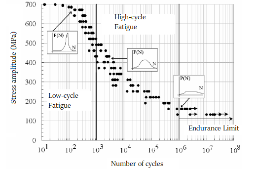
Figure 2: S-N curve

The campaign results are then used to study fatigue resistance and are represented graphically in an S-N scale (see figure 2). S-N curves highlight the existence of three fatigue regimes. Firstly, low cycle fatigue corresponds to short lives associated with high levels of stress. Secondly, during high cycle fatigue, the number of cycles to failure decreases log-linearily with respect to the loading. The last regime is the endurance limit, in which failure occurs at a very high number of cycles or doesn’t occur at all. We will focus in the following on the endurance limit, which is also the hardest regime to characterize since there is usually only few and scattered observations.

In this framework, we are focusing on minimal risk. The critical quantities that are used to characterize minimal risk linked to fatigue damage are failure quantiles, called in this framework allowable stresses at a given number of cycles and for a fixed level of probability. Those quantiles are of great importance since they intervene in decisions pertaining engine parts dimensioning, pricing decisions as well as maintenance policies.

1.2 Formalization of the industrial problem

The aim of this study is to propose a new design method for the characterization of allowable stress in very high cycle fatigue, for a very low risk $\alpha$ of order $10^{-3}$. We are willing to obtain a precise estimation method of the $\alpha-$failure quantile based on a minimal number of trials.

Denote $N$ the lifetime of a material in terms of number of cycles to failure and $S$ the stress amplitude of the loading, in MPa. Let $n_{0}$ be the targeted time span of order $10^{6}-10^{7}$ cycles.

Define the allowable stress $s_{\alpha}$ at $n_{0}$ cycles and level of probability $\alpha$ $=10^{-3}$ the level of stress that guarantee that the risk of failure before $n_{0}$ does not exceed $\alpha$:

$$s_{\alpha}=\sup\left\{s:\mathbb{P}(N\leq n_{0}|S=s)\leq\alpha\right\}$$ (1)

We will now introduce a positive r.v. $R=R_{n_{0}}$ modeling the resistance of the material at $n_{0}$ cycles and homogeneous to the stress. $R$ is the variable of interest in this study and its distribution $\mathbb{P}$ is defined as:

$$\mathbb{P}(R\leq s)=\mathbb{P}(N\leq n_{0}|S=s).$$ (2)

Thus, the allowable stress can be rewritten as the $\alpha-$quantile of the distribution of $R$,

$$s_{\alpha}=q_{\alpha}=\sup\left\{s:\mathbb{P}(R\leq s)\leq\alpha\right\}.$$ (3)

However, $R$ is not directly observed. Indeed, the usable data collected at the end of a test campaign consists in couples of censored fatigue life - stress levels $\left(\min(N,n_{0}),s\right)$ where $s$ is part of the design of the experiment. The relevant information that can be drawn from those observations to characterize $R$ is restricted to indicators of whether or not the specimen tested has failed at $s$ before $n_{0}$. Therefore, the relevant observations corresponding to a campaign of $n$ trials are formed by a sample of variables $Y_{1},...,Y_{n}$ with for $1\leq i\leq n,$

$$Y_{i}=\left\{\begin{array}[]{l}1\text{ if }R_{i}\leq s_{i}\\ 0\text{ if }R_{i}>s_{i}\end{array}\right.$$

where $s_{i}$ is the stress applied on specimen $i.$

Note that the number of observations is constrained by industrial and financial considerations; Thus $\alpha$ is way lower than $1/n$ and we are considering a quantile lying outside the sample range.

While we motivate this paper with the above industrial application, note that this kind of problem is of interest in other domains, such as broader reliability issues or medical trials through the estimation of the maximum tolerated dose of a given drug.

2 Extreme quantile estimation, a short survey

As seen above estimating the minimal admissible constraint raises two issues; on one hand the estimation of an extreme quantile, and on the other hand the need to proceed to inference based on exceedances under thresholds.  We present a short exposition of these two areas, keeping in mind that the literature on extreme quantile estimation deals with complete data, or data under right censoring.

2.1 Extreme quantiles estimation methods

Extreme quantile estimation in the univariate setting is widely covered in the literature when the variable of interest $X$ is either completely or partially observed.

The usual framework is the study of the $(1-\alpha)-$quantile of a r.v $X$, with very small $\alpha$.

The most classical case corresponds to the setting where ${x}_{1-\alpha}$ is drawn from a $n$ sample of observations $X_{1},\dots X_{n}$. We can distinguish estimation of high quantile, where $x_{1-\alpha}$ lies inside the sample range, see Weissman 1978 [22] and Dekkers and al. 1989 [6], and the estimation of an extreme quantile outside the boundary of the sample, see for instance De Haan and Rootzén 1993 [5]. It is assumed that $X$ belongs to the domain of attraction of an extreme value distribution. The tail index of the latter is then estimated through maximum likelihood (Weissman 1978 [22]) or through an extension of Hill’s estimator (see the moment estimator by Dekkers and al. 1989 [6]). Lastly, the estimator of the quantile is deduced from the inverse function of the distribution of the $k$ largest observations. Note that all the above references assume that the distribution has a Pareto tail. An alternative modeling has been proposed by De Valk 2016 [7] and De Valk and Cai 2018 [8], and consists in assuming a Weibull type tail, which enables to release some second order hypotheses on the tail. This last work deals with the estimation of extreme quantile lying way outside the sample range and will be used as a benchmark method in the following sections.

Recent studies have also tackled the issue of censoring. For instance, Beirlant and al. 2007 [2] and Einmahl and al. 2008 [13] proposed a generalization of the peak-over-threshold method when the data are subjected to random right censoring and an estimator for extreme quantiles. The idea is to consider a consistent estimator of the tail index on the censored data and divide it by the proportion of censored observations in the tail. Worms and Worms 2014 [23] studied estimators of the extremal index based on Kaplan Meier integration and censored regression.

However the literature does not cover the case of complete truncation, i.e when only exceedances over given thresholds are observed. Indeed, all of the above are based on estimations of the tail index over weighed sums of the higher order statistics of the sample, which are not available in the problem of interest in this study. Classical estimation methods of extreme quantiles are thus not suited to the present issue.

In the following, we study designs of experiment at use in industrial contexts and their possible application to extreme quantiles estimation.

2.2 Sequential design based on dichotomous data

In this section we review two standard methods in the industry and in biostatistics, which are the closest to our purpose. Up to our knowledge, no technique specifically addresses inference for extreme quantiles.

We address the estimation of small quantiles, hence the events of interest are of the form $\left(R<s\right)$ and the quantile is $q_{\alpha}$ for small $\alpha.$

The first method is the staircase, which is the present tool used to characterize a material fatigue strength.

The second one is the Continual Reassessment Method (CRM) which is adapted for assessing the admissible toxicity level of a drug in Phase 1 clinical trials.

Both methods rely on a parametric model for the distribution of the strength variable $R.$ We have considered two specifications, which allow for simple comparisons of performance, and do not aim at an accurate modelling in safety.

2.2.1 The Staircase method

Denote $\mathbb{P}(R\leq s)=\phi(s,\theta_{0})$. Invented by Dixon and Mood (1948 [10]), this technique aims at the estimation of the parameter $\theta_{0}$ through sequential search based on data of exceedances under thresholds. The procedure is as follows.

Procedure

Fix

• The initial value for the constraint, $S_{ini}$,

• The step $\delta>0$,

• The number of cycles $n_{0}$ to perform before concluding a trial,

• The total number of items to be tested, $K$.

The first item is tested at level $s_{(1)}=S_{ini}$. The next item is tested at level $s_{(2)}=S_{ini}-\delta$ in case of failure and $s_{(2)}=S_{ini}+\delta$ otherwise. Proceed sequentially on the $K-2$ remaining specimen at a level increased (respectively decreased) by $\delta$ in case of survival (resp. failure). The process is illustrated in figure 3.

Note that the proper conduct of the Staircase method relies on strong assumptions on the choice of the design parameters. Firstly, $S_{ini}$ has to be sufficiently close to the expectation of $R$ and secondly, $\delta$ has to lay between $0.5\sigma$ and $2\sigma$, where $\sigma$ designates the standard deviation of the distribution of $R$.

Denote $\mathbb{P}(R\leq s)=\phi(s,\theta_{0})$ and $Y_{i}$ the variable associated to the issue of the trial $i$, $1\leq i\leq K$, where $Y_{i}$ takes value $1$ under failure and $0$ under no failure, $Y_{i}=\mathds{1}_{N_{a}\leq n_{0}}\sim\mathcal{B}(\phi(s_{i},\theta_{0}))$.

Figure 3: Staircase procedure

Estimation

After the $K$ trials, the parameter $\theta_{0}$ is estimated through maximization of the likelihood, namely

$$\widehat{\theta}=\underset{\theta}{\text{argmax}}{\prod_{i=1}^{K}\phi(s_{i},\theta)^{y_{i}}(1-\phi(s_{i},\theta))^{(1-y_{i})}}.$$ (4)

Numerical results

The accuracy of the procedure has been evaluated on the two models presented below on a batch of 1000 replications, each with $K=100.$

Exponential case

Let $R\sim\mathcal{E}(\lambda)$ with $\lambda=0.2$. The input parameters are $S_{\text{ini}}=5$ and $\delta=15\in\left[0.5\times\frac{1}{\lambda^{2}},2\times\frac{1}{\lambda^{2}}\right]$.

As shown in Table 1, the relative error pertaining to the parameter $\lambda$ is roughly $25\%$, although the input parameters are somehow optimal for the method. The resulting relative error on the $10^{-3}$ quantile is $40\%.$ Indeed the parameter $\lambda$ is underestimated, which results in an overestimation of the variance $1/\lambda^{2}$ , which induces an overestimation of the $10^{-3}$ quantile.

Relative error
On the parameter		On $s_{\alpha}$
Mean	Std	Mean	Std
-0.252	0.178	0.4064874	0.304

Table 1: Results obtained using the Staircase method through simulations under the exponential model.

Gaussian case

We now choose $R\sim\mathcal{N}(\mu,\sigma)$ with $\mu=60$ and $\sigma=10$. The value of $S_{\text{ini}}$ is set to the expectation and $\delta=7$ belongs to the interval $\left[\frac{\sigma}{2},2\sigma\right].$ The same procedure as above is performed and yields the results in Table 2.

Relative error
On $\mu$		On $\sigma$		On $s_{\alpha}$
Mean	Std	Mean	Std	Mean	Std
-0.059	0.034	1.544	0.903	-1.753	0.983

Table 2: Results obtained using the Staircase method through simulations under the Gaussian model.

The expectation of $R$ is recovered rather accurately, whereas the estimation of the standard deviation suffers a loss in accuracy, which in turn yields a relative error of 180 %  on the $10^{-3}$ quantile.

Drawback of the Staircase method

A major advantage of the Staircase lies in the fact that the number of trials to be performed in order to get a reasonable estimator of the mean is small. However, as shown by the simulations, this method is not adequate for the estimation of extreme quantiles. Indeed, the latter follows from an extrapolation based on estimated parameters, which furthermore may suffer of bias. Also, reparametrization of the distribution making use of the theoretical extreme quantile would not help, since the estimator would inherit of a large lack of accuracy.

2.2.2 The Continuous Reassesment Method (CRM)

General principle

The CRM (O’Quigley, Pepe and Fisher, 1990[18]) has been designed for clinical trials and aims at the estimation of $q_{\alpha}$ among $J$ stress levels $s_{1},...,s_{J}$, when $\alpha$ is of order $20\%$.

Denote $\mathbb{P}(R\leq s)=\psi(s,\beta_{0})$. The estimator of $q_{\alpha}$ is

$$s^{\ast}:=\underset{s_{j}\in\{s_{1},...,s_{J}\}}{\text{arginf}}{|\psi(s_{j},\beta_{0})-\alpha|}.$$

This optimization is performed iteratively and $K$ trials are performed at each iteration.

Start with an initial estimator $\widehat{\beta_{1}}$ of $\beta_{0}$, for example through a Bayesian choice as proposed in [18]. Define

$$s_{1}^{\ast}:=\underset{s_{j}\in\{s_{1},...,s_{J}\}}{\text{arginf}}{|\psi(s_{j},\widehat{\beta_{1}})-\alpha|}.$$

Every iteration follows a two-step procedure:

Step 1. Perform $J$ trials under $\psi(.,\beta_{0})$, say $R_{1,1},..,R_{1,J}$ and observe only their value under threshold, say $Y_{1,j}:={\Large 1}_{R_{1,j}<s_{1}^{\ast}},1\leq j\leq J.$

Step i. Iteration $i$ consists in two steps :

• Firstly an estimate $\widehat{\beta_{i}}$ of $\beta_{0}$ is produced on the basis of the information beared by the trials performed in all the preceding iterations through maximum likelihood under $\psi(.,\beta_{0})$ (or by maximizing the posterior distribution of the parameter).

• $$s_{i}^{\ast}:=\underset{s_{j}\in\{s_{1},...,s_{J}\}}{\text{arginf}}{|\psi(s,}\widehat{{\beta_{i}}}{)-\alpha|};$$

  This stress level $s_{i}^{\ast}$ is the one under which the next $K$ trials $Y_{i,1},\dots,Y_{i,K}$ will be performed in the Bernoulli scheme $\mathcal{B}\left(\psi(s_{i}^{\ast},\beta_{0})\right)$.

The stopping rule depends on the context (maximum number of trials or stabilization of the results).

Note that the bayesian inference is useful in the cases where there is no diversity in the observations at some iterations of the procedure, i.e when, at a given level of test $s_{i}^{*}$, only failures or survivals are observed.

Application to fatigue data

The application to the estimation of the minimal allowable stress is treated in a bayesian setting. We do not directly put a prior on the parameter $\beta_{0}$, but rather on the probability of failure. We consider a prior information of the form: at a given stress level $s$, we can expect $k$ failures out of $n$ trials. Denote $\pi_{s}$ the prior indexed on the stress level $s$. $\pi_{s}$ models the failure probability at level $s$ and has a Beta distribution given by

$$\pi_{s}\sim\beta(k,n-k+1).$$ (5)

Let $R$ follow an exponential distribution: $\forall s\geq 0,\psi(s,\beta_{0})=p_{s}=1-\exp(-\beta_{0}s)$.

It follows $\forall s,~{}\beta_{0}=-\frac{1}{s}\log(1-p_{s})$.

Define the random variable $\Lambda_{s}=-\frac{1}{s}\log(1-\pi_{s})$ which, by definition of $\pi_{s}$, is distributed as an k-order statistic of a uniform distribution $U_{k,n}$.

The estimation procedure of the CRM is obtained as follows:

Step 1. Compute an initial estimator of the parameter

$$\Lambda_{s}=\frac{1}{L}\sum_{l=1}^{L}-\frac{1}{s}\log(1-\pi_{s}^{l})$$

with $\pi_{s}^{l}\sim\beta(k,n-k+1),1\leq l\leq L$. Define

$$s_{1}^{\ast}:=\underset{s_{j}\in\{s_{1},...,s_{J}\}}{\text{arginf}}{|(1-\exp(-\Lambda_{s}s_{j}))-\alpha|}.$$

and perform $J$ trials at level $s_{1}^{\ast}$. Denote the observations $Y_{1,j}:={\Large 1}_{R_{1,j}<s_{1}^{\ast}},1\leq j\leq J.$

Step i. At iteration $i$, compute the posterior distribution of the parameter:

$$\pi^{*}_{s_{i}}\sim\beta\left(k+\sum_{l=1}^{i}\sum_{j=1}^{J}Y_{l,j}~{},~{}n+(J\times i)-(k+\sum_{l=1}^{i}\sum_{j=1}^{J}Y_{l,j})+1\right)$$ (6)

The above distribution also corresponds an order statistic of the uniform distribution $U_{k+\sum_{l=1}^{i}\sum_{j=1}^{J}Y_{l,j}~{},~{}n+(J\times i)}$. We then obtain an estimate $\Lambda_{s_{1}^{\ast}}$.

The next stress level $s_{i+1}^{\ast}$ to be tested in the procedure is then given by

$$s_{i+1}^{\ast}:=\underset{s_{j}\in\{s_{1},...,s_{J}\}}{\text{arginf}}{|(1-\exp(-\Lambda_{s_{1}^{\ast}}s_{j}))-\alpha|}.$$

Numerical simulation for the CRM

Under the exponential model with parameter $\lambda=0.2$ and through $N=10$ iterations of the procedure, and $J=10$, with equally distributed thresholds $s_{1},..,s_{J}$ , and performing $K=50$ trials at each iteration, the results in Table 3 are obtained.

Relative error
On the $0.1-$quantile		On the $10^{-3}-$quantile
Mean	Std	Mean	Std
0.129	0.48	-0.799	0.606

Table 3: Results obtained through CRM on simulations for the exponential model

The $10^{-3}-$quantile is poorly estimated on a fairly simple model. Indeed for thresholds close to the expected quantile, nearly no failure is observed. So, for acceptable $K$, the method is not valid; figure 4 shows the increase of accuracy with respect to $K.$

Both the Staircase and the CRM have the same drawback in the context of extreme quantile estimation, since the former targets the central tendency of the variable of interest and the latter aims at the estimation of quantiles of order 0.2 or so, far from the target $\alpha=10^{-3}$. Therefore, we propose an original procedure designed for the estimation of extreme quantiles under binary information.

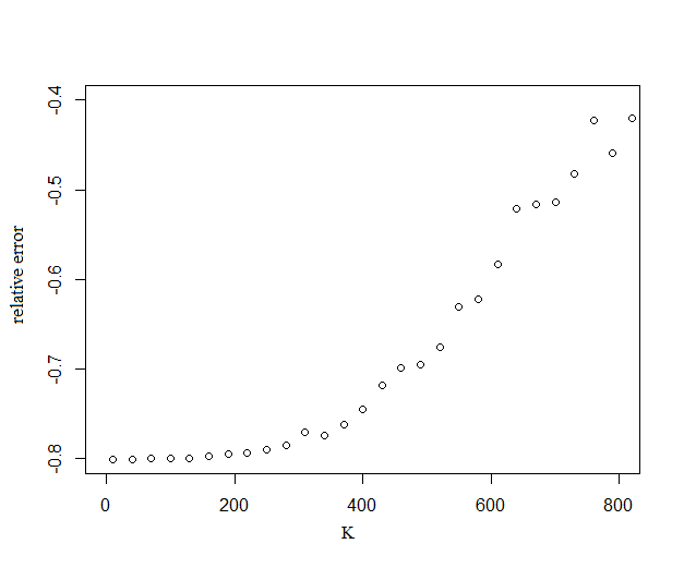
Figure 4: Relative error on the $10^{-3}$-quantile with respect to the number of trials for each stress level

3 A new design for the estimation of extreme quantiles

3.1 Splitting

The design we propose is directly inspired by the general principle of Splitting methods used in the domain of rare events simulation and introduced by Kahn and Harris (1951 [16]).

The idea is to overcome the difficulty of targeting an extreme event by decomposing the initial problem into a sequence of less complex estimation problem. This is enabled by the splitting methodology which decompose a small probability into the product of higher order probabilities.

Denote $\mathbb{P}$ the distribution of the r.v. $R$. The event $\{R\leq s_{\alpha}\}$ can be expressed as the intersection of inclusive events  for $s_{\alpha}=s_{m}<s_{m-1}<...<s_{1}$ it holds:

$$\{R\leq s_{\alpha}\}=\{R\leq s_{m}\}\subset\dots\subset\{R\leq s_{1}\}.$$

It follows that

$$\mathbb{P}(R\leq s_{\alpha})=\mathbb{P}(R\leq s_{1})\prod_{j=1}^{m-1}\mathbb{P}(R\leq s_{j+1}\mid R\leq s_{j})$$ (7)

The thresholds $(s_{j})_{j=1,\dots,m}$ should be chosen such that all $\mathbb{P}(R\leq s_{j+1}\mid R\leq s_{j})_{j=1,\dots,m}$ be of order $p=0.2$ or 0.3, in such a way that $\left\{R\leq s_{j+1}\right\}$ is observed in experiments performed under the conditional distribution of $R$ given $\left\{R\leq s_{j}\right\}$, and in a way which makes $\alpha$ recoverable by a rather small number of such probabilities $\mathbb{P}(R\leq s_{j+1}\mid R\leq s_{j})$ making use of (7).

From the formal decomposition in (7), a practical experimental scheme can be deduced. Its form is given in algorithm 1.

Procedure 1 Splitting procedure

  Initialization

  Fix

• $\left.\text{\parbox{260.17464pt}{ \par\itemize@item@[$\bullet$] the number $m$ of iterations to be performed (and of levels to be tested); \par\itemize@item@[$\bullet$] the level of conditional probabilities $p$ (laying between 20 and 30 \%); }}\right\}$     such that $p^{m}\approx\alpha$

• the first tested level $s_{1}$ (ideally the $p-$quantile of the distribution of $R$);

• the number $K$ of trials to be performed at each iteration.

  First step

• $K$ trials are performed at level $s_{1}$. The observations are the indicators of failure $Y_{1,1},\dots,Y_{1,K}$, where $Y_{1,i}=\mathds{1}(R_{1,i}<s_{1})$ of distribution $\mathcal{B}\left(\mathbb{P}(R\leq s_{1})\right)$.

• Determination of $s_{2}$, $p-$quantile of the truncated distribution $R\mid R\leq s_{1}$.

  Iteration $j=2$ to $m$

• $K$ trials are performed at level $s_{j}$ under the truncated distribution of $R\mid R\leq s_{j-1}$ resulting to observations $Y_{j,1},\dots,Y_{j,k}\sim\mathcal{B}\left(\mathbb{P}(R\leq s_{j}\mid R\leq s_{j-1})\right)$.

• Determination of $s_{j+1}$, the $p-$quantile of $R\mid R\leq s_{j}$.

  The last estimated quantile $s_{m}$ provides the estimate of $s_{\alpha}$.

3.2 Sampling under the conditional probability

In practice batches of specimen are put under trial, each of them with a decreasing strength; this allows to target the tail of the distribution $\mathbb{P}$ iteratively.

Figure 5: Sampling under the strengh density at $n_{0}$ cycles

In other words, in the first step, points are sampled in zone (I). Then in the following step, only specimen with strength in zone II are considered, and so on. In the final step, the specimen are sampled in zone IV. At level $s_{m}$, they have a very small probability to fail before $n_{0}$ cycles under $\mathbb{P}$, however under their own law of failure, which is $\mathbb{P}(\mathbf{.}\mid R\leq s_{m-1})$, they have a probability of failure of order 0.2.

In practice, sampling in the tail of the distribution is achieved by introducing flaws in the batches of specimens. The idea is that the strength of the material varies inversely with respect to the size of the incorporated flaws. The flaws are spherical and located inside the specimen (not on its surface). Thus, as the procedure moves on, the trials are performed on samples of materials incorporating flaws of greater diameter. This procedure is based on the hypothesis that there is a correspondence between the strength of the material with flaw of diameter $\theta$ and the truncated strength of this same material without flaw under level of stress $s^{*}$, i.e. we assume that noting $R_{\theta}$ the strength of the specimen with flaw of size $\theta$, it holds that there exists $s^{*}$ such that

$$\mathcal{L}(R_{\theta})\approx\mathcal{L}(R\mid R\leq s^{*}).$$

Before launching a validation campaign for this procedure, a batch of 27 specimen has been machined including spherical defects whose sizes vary between 0 and 1.8mm (see Figure 6). These first trials aim at estimating the decreasing relation between mean allowable stress and defects diameter $\theta$. This preliminary study enabled to draw the abatement fatigue curve as a function of $\theta$, as shown in Figure 7.

Figure 6: Coupons incorporating spherical defects of size varying from 0 mm (on the left) to 1.8 mm (on the right)

Figure 7: Mean allowable stress with respect to the defect size

Results in Figure 7 will be used during the splitting procedure to select the diameter $\theta$ to be incorporated in the batch of specimens tested at the current iteration as reflecting the sub-population of material of smaller resistance.

3.3 Modeling the distribution of the strength, Pareto model

The events under consideration have small probability under $\mathbb{P}.$ By (7) we are led to consider the limit behavior of conditional distributions under smaller and smaller thresholds, for which we make use of classical approximations due to Balkema and de Haan (1974[1]) which stands as follows, firstly in the commonly known setting of exceedances over increasing thresholds. Denote $\widetilde{R}:=1/R$.

Theorem 1.

For $\widetilde{R}$ of distribution $F$ belonging to the maximum domain of attraction of an extreme value distribution with tail index $c$, i.e. $F\in MDA(c)$, it holds that: There exists $a=a(s)>0$, such that:

$$\lim\limits_{s\rightarrow\infty}\sup_{0\leq x<\infty}\left\lvert\frac{1-F\left(x+s\right)}{1-F\left(s\right)}-\left(1-G_{(c,a}(x)\right)\right\rvert=0$$

where $G_{(c,a)}$ is defined through

$$G_{(c,a)}(x)=1-\exp\left\{-\int_{0}^{\frac{x}{a}}\left[(1+ct)_{+}\right]^{-1}dt\right\}$$

where $a>0$ and $c\in\mathbb{R}$.

The distribution $G$ is the Generalized Pareto distribution $GPD(c,a)$ is defined explicitly through

$$1-G(x)=\left\{\begin{array}[]{l}(1+\frac{c}{a}x)^{-1/c}\text{ when }c\neq 0\\ \exp(-\frac{x}{a})\text{ when }c=0\end{array}\right.$$

where $x\geq 0$ for $c\geq 0$ and $0\leq x\leq-\frac{a}{c}$ if $c<0.$

Generalized Pareto distributions enjoy invariance through threshold conditioning, an important property for our sake. Indeed it holds, for $\widetilde{R}\sim GDP(c,a)$ and $x>s$,

$$\mathbb{P}\left(\widetilde{R}>x\mid\widetilde{R}>s\right)=\left(1+\frac{c(x-s)}{a+cs}\right)^{-1/c}$$ (8)

We therefore state:

Proposition 2.

When $\widetilde{R}\sim GPD(c,a)$ then, given $\left(\widetilde{R}>s\right)$, the r.v. $\widetilde{R}-s$ follows a $GPD(c,a+cs)$.

The GPD’s are on the one hand stable under thresholding and on the other appear as the limit distribution for thresholding operations. This chain of arguments is quite usual in statistics, motivating the recourse to the ubiquous normal or stable laws for additive models. This plays in favor of GPD’s as modelling the distribution of $\widetilde{R}$ for excess probability inference. Due to the lack of memory property, the exponential distribution which appears as a possible limit distribution for excess probabilities in Theorem 1 do not qualify for modelling. Moreover since we handle variables $R$ which can approach $0$ arbitrarily (i.e. unbounded $\widetilde{R}$) the parameter $c$ is assumed positive.

Turning to the context of the minimal admissible constraint, we make use of the r.v. $R=1/\widetilde{R}$ and proceed to the corresponding change of variable.

When $c>0$, the distribution function of the r.v. $R$ writes for nonnegative $x$:

$$F_{c,a}(x)=(1+\frac{c}{ax})^{-1/c}.$$ (9)

For $0<x<u$, the conditional distribution of $R$ given $\left\{R<u\right\}$ is

$$\mathbb{P}(R<x\mid R<u)=\left(1-\frac{c(\frac{1}{x}-\frac{1}{u})}{a+\frac{c}{u}}\right)^{-1/c}$$

which proves that the distribution of $R$ is stable under threshold conditioning with parameter $\left(a_{u},c\right)$ with

$$a_{u}=a+\frac{c}{u}.$$ (10)

In practice at each step $j$ in the procedure the stress level $s_{j}$ equals the corresponding threshold $1/\widetilde{s}_{j}$ , a right quantile of the conditional distribution of $\widetilde{R\text{ }}$ given $\left\{\widetilde{R}>\widetilde{s}_{j-1}\right\}$. Therefore the observations take the form $Y_{i}=\mathds{1}_{R_{i}<s_{j-1}}=\mathds{1}_{\widetilde{R}_{i}>\widetilde{s}_{j-1}},~{}~{}i=1,\dots,K_{j}$.

A convenient feature of model (9) lies in the fact that the conditional distributions are completely determined by the initial distribution of $R$ , therefore by $a\$ and $c.$ The parameters $a_{j}$ of the conditional distributions are determined from these initial parameters and by the corresponding stress level $s_{j};$ see (10).

3.4 Notations

The distribution function of the r.v. $\widetilde{R}$ is a $GPD(c_{T},a_{T})$ of distrubution function $G_{(c_{T},a_{T})}.$ Note $\overline{G}_{(c_{T},a_{T})}=1-G_{(c_{T},a_{T})}.$

Our proposal relies on iterations. We make use of a set of thresholds $(\widetilde{s}_{1},...,\widetilde{s}_{m})$ and define for any $j\in\{1,...,m\}$

$$G_{(c_{j},a_{j})}(x-\widetilde{s}_{j})=\mathbb{P(}\left.\widetilde{R}>x\right|\widetilde{R}>\widetilde{s}_{j})$$

with $c_{j}=c_{T}$ and $a_{j}=a_{T}+c_{T}\widetilde{s}_{j}$ where we used (8).

At iteration $j$, denote $(\widehat{c},\widehat{a})_{j}$ the estimators of $(c_{j},a_{j})$.Therefore $1-G_{(\widehat{c},\widehat{a})_{j}}(x-\widetilde{s}_{j})$ estimates $\mathbb{P(}\left.\widetilde{R}>x\right|\widetilde{R}>\widetilde{s}_{j})$. Clearly, estimators of $(c_{T},a_{T})$ can be recovered from $(\widehat{c},\widehat{a})_{j}$ through $\widehat{c}_{T}=\widehat{c}$ and $\widehat{a}_{T}=\widehat{a}-\widehat{c}~{}\widetilde{s}_{j}.$

3.5 Sequential design for the extreme quantile estimation

Fix $m$ and $p$ , where $m$ denotes the number of stress levels under which the trials will be performed, and $p$ is such that $p^{m}=\alpha.$

Set a first level of stress, say $s_{1}$ large enough (i.e. $\widetilde{s}_{1}=1/s_{1}$ small enough) so that $p_{1}=\mathbb{P}(R<s_{1})$ is large enough and perform trials at this level. The optimal value of $s_{1}$ should satisfy $p_{1}=p$, which cannot be secured. This choice is based on expert advice.

Turn to $\widetilde{R}:=1/R$. Estimate $c_{T}$ and $a_{T}$, for the GPD $\left(c_{T},a_{T}\right)$ model describing $\widetilde{R}$, say $(\widehat{c},\widehat{a})_{1}$, based on the observations above $\widetilde{s}_{1}$ (note that under $s_{1}$ the outcomes of $R$ are easy to obtain, since the specimen is tested under medium stress).

Define

$$\widetilde{s}_{2}:=\sup\left\{s:\overline{G}_{(\widehat{c},\widehat{a})_{1}}\left(s-\widetilde{s}_{1}\right)<p\right\}$$

the $(1-p)-$quantile of $G_{(\widehat{c},\widehat{a})_{1}}.$ $\widetilde{s}_{2}$ is the level of stress to be tested at the following iteration.

Iterating from step $j=2$ to $m-1$, perform $K$ trials under $G_{(c_{1},a_{1})}$ say $\widetilde{R}_{j,1},..,\widetilde{R}_{j,K}$ and consider the observable variables $Y_{j,i}:={\Large 1}_{\widetilde{R}_{j,i}>\widetilde{s}_{j}}$. Therefore the $K$ iid replications $Y_{j,1},..,Y_{j,K}$ follow a Bernoulli $\mathcal{B}(\overline{G}_{({c}_{j-1},{a}_{j-1})}\left(\widetilde{s}_{j}-\widetilde{s}_{j-1}\right))$, where $\widetilde{s}_{j}$ has been determined at the previous step of the procedure. Estimate $(c_{j},a_{j})$ in the resulting Bernoulli scheme, say $(\widehat{c},\widehat{a})_{j}$. Then define

$$\begin{split}\widetilde{s}_{j+1}&:=\sup\left\{s:\overline{G}_{(\widehat{c},\widehat{a})_{j}}\left(s-\widetilde{s}_{j}\right)<p\right\}\\ &=G_{\left(\widehat{c},\widehat{a}\right)_{j}}^{-1}(1-p)+\widetilde{s}_{j},\end{split}$$

which is the $(1-p)-$quantile of the estimated conditional distribution of $\widetilde{R}$ given $\{\widetilde{R}>\widetilde{s_{j}}\}$, i.e. $G_{(\widehat{c},\widehat{a})_{j}}$, and the next level to be tested.

In practice a conservative choice for $m$ is given by $m=\left\lceil\frac{log\alpha}{logp}\right\rceil$, where $\lceil.\rceil$ denotes the ceiling function. This implies that the attained probability $\widetilde{\alpha}$ is less than or equal to $\alpha.$

The $m$ stress levels $\widetilde{s}_{1}<\widetilde{s}_{1}<\dots<\widetilde{s}_{m}=\widetilde{q}_{1-\alpha}$ satisfy

$$\begin{split}\widetilde{\alpha}&=\overline{G}(\widetilde{s}_{1})\prod_{j=1}^{m-1}\overline{G}_{\left(\widehat{c},\widehat{a}\right)_{j}}(\widetilde{s}_{j+1}-\widetilde{s}_{j})\\ &={p}_{1}p^{m-1}\end{split}$$

Finally by its very definition $\widetilde{s}_{m}$ is a proxy of $\widetilde{q}_{1-\alpha}.$

Although quite simple in its definition, this method bears a number of drawbacks, mainly in the definition of $\left(\widehat{c},\widehat{a}\right)_{j}.$ The next section addresses this question.

4 Sequential enhanced design in the Pareto model

In this section we focus on the estimation of the parameters $\left(c_{T},a_{T}\right)$ in the $GPD(c_{T},a_{T})$ distribution of $\widetilde{R}.$ One of the main difficulties lies in the fact that the available information does not consist of replications of the r.v. $\widetilde{R}$ under the current conditional distribution $G_{(c_{j},a_{j})}$ of $\widetilde{R}$ given $\left(\widetilde{R}>\widetilde{s_{j}}\right)$ but merely on very downgraded functions of those.

At step $j$ we are given $G_{(\widehat{c},\widehat{a})_{j}}$ and define $\widetilde{s}_{j+1}$ as its $\left(1-p\right)-$quantile. Simulating $K$ r.v. $\widetilde{R}_{j,i}$ with distribution $G_{(c_{j},a_{j})}$, the observable outcomes are the Bernoulli ($p$) r.v.’s $Y_{j,i}:=1_{\widetilde{R}_{j,i}>\widetilde{s}_{j+1}}.$ This loss of information with respect to the $\widetilde{R}_{j,i}$ ’s makes the estimation step for the coefficients $(\widehat{c},\widehat{a})_{j+1}$ quite complex; indeed $(\widehat{c},\widehat{a})_{j+1}$ is obtained through the $Y_{j,i}$’s, $1\leq i\leq K$.

It is of interest to analyze the results obtained through standard Maximum Likelihood Estimation of $(\widehat{c},\widehat{a})_{j+1}.$ The quantile $\widetilde{q}_{1-\alpha}$ is loosely estimated for small $\alpha$; as measured on 1000 simulation runs, large standard deviation of $\widehat{\widetilde{q}}_{1-\alpha}$ is due to poor estimation of the iterative parameters $(\widehat{c},\widehat{a})_{j+1}.$ We have simulated $n=200$ realizations of r.v.’s $Y_{i}$ with common Bernoulli distribution with parameter $\overline{G}_{\left(c_{T},a_{T}\right)}(\widetilde{s}_{1}).$ Figure 8 shows the log likelihood function of this sample as the parameter of the Bernoulli $\overline{G}_{\left(c^{\prime},a^{\prime}\right)}(\widetilde{s_{0}})$ varies according to $\left(c^{\prime},a^{\prime}\right).$ As expected this function is nearly flat in a very large range of $\left(c^{\prime},a^{\prime}\right).$

This explains the poor results in Table 5 obtained through the Splitting procedure when the parameters at each step are estimated by maximum likelihood, especially in terms of dispersion of the estimations. Moreover, the accuracy of the estimator of $\widetilde{q}_{1-\alpha}$ quickly decreases with the number $K$ of replications $Y_{j,i}$, $1\leq i\leq K$.

Changing the estimation criterion by some alternative method does not improve significantly; Figure 9 shows the distribution of the resulting estimators of $\widetilde{q}_{1-\alpha}$ for various estimation methods (minimum Kullback Leibler, minimum Hellinger and minimum L1 distances - see their definitions in Appendix LABEL:div) of $\left(c_{T},a_{T}\right).$

This motivates the need for an enhanced estimation procedure.

Minimum	Q25	Q50	Mean	Q75	Maximum
67.07	226.50	327.40	441.60	498.90	10 320.00

Table 4: Estimation of the $(1-\alpha)-$quantile, $\widetilde{s}_{\alpha}=469.103$, through procedure 3.5 with $K=50$

	$\widetilde{s}_{m}$ for $K=30$		$\widetilde{s}_{m}$ for $K=50$
$\widetilde{s}_{\alpha}$	Mean	Std	Mean	Std
469.103	1 276.00	12 576.98	441.643	562.757

Table 5: Estimation of the $(1-\alpha)-$quantile, $\widetilde{s}_{\alpha}=469.103$, through procedure 3.5 for different values of $K$

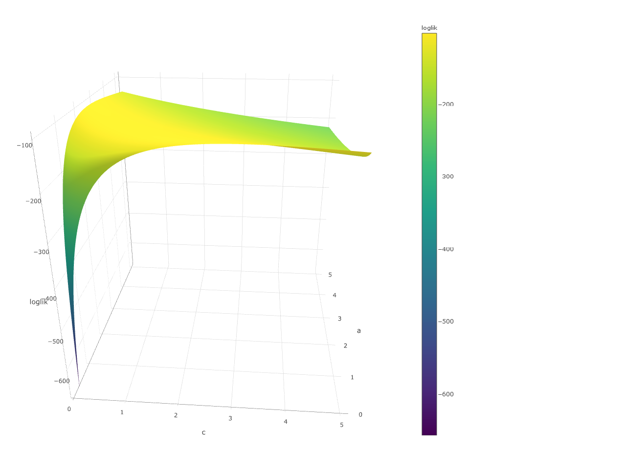
Figure 8: Log-likelihood of the Pareto model with binary data

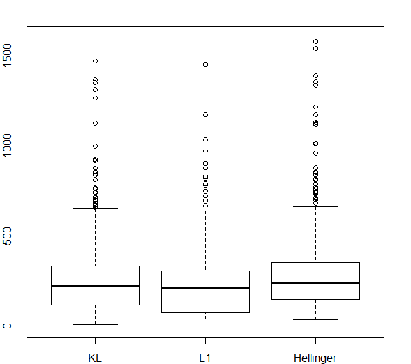
Figure 9: Estimations of the $\alpha-$quantile based on the Kullback-Leibler, L1 distance and Hellinger distance criterion

4.1 An enhanced sequential criterion for estimation

We consider an additional criterion which makes a peculiar use of the iterative nature of the procedure. We will impose some control on the stability of the estimators of the conditional quantiles through the sequential procedure.

At iteration $j-1$, the sample $Y_{j-1,i}$ , $1\leq i\leq K$ has been generated under $G_{(\widehat{c},\widehat{a})_{j-2}\text{ }}$and provides an estimate of $p$ through

$$\widehat{p}_{j-1}:=\frac{1}{K}\sum_{i=1}^{n}Y_{j-1,i}.$$ (11)

The above $\widehat{p}_{j-1}$ estimates $\mathbb{P}\left(\widetilde{R}>\widetilde{s}_{j-1}\mid\widetilde{R}>\widetilde{s}_{j-2}\right)$ conditionally on $\widetilde{s}_{j-1}$ and $\widetilde{s}_{j-2}.$ We write this latter expression $\mathbb{P}\left(\widetilde{R}>\widetilde{s}_{j-1}\mid\widetilde{R}>\widetilde{s}_{j-2}\right)$ as a function of the parameters obtained at iteration $j$ , namely $(\widehat{c},\widehat{a})_{j}.$The above r.v’s $\ Y_{j-1,i}$ stem from variables $\widetilde{R}_{j-1,i}$ greater than $\ \widetilde{s}_{j-2}.$ At step $j,$ estimate then $\mathbb{P}\left(\widetilde{R}>\widetilde{s}_{j-1}\mid\widetilde{R}>\widetilde{s}_{j-2}\right)$ making use of $G_{(\widehat{c},\widehat{a})_{j}}.$ This backward estimator writes

$$\frac{\overline{G}_{(\widehat{c},\widehat{a})_{j}}(\widetilde{s}_{j-1})}{\overline{G}_{(\widehat{c},\widehat{a})_{j}}(\widetilde{s}_{j-2})}=1-G_{(\widehat{c},\widehat{a})_{j}}(\widetilde{s}_{j-1}-\widetilde{s}_{j-2}).$$

The distance

$$\left|\left(\overline{G}_{(\widehat{c},\widehat{a})_{j}}(\widetilde{s}_{j-1}-\widetilde{s}_{j-2})\right)-\widehat{p_{j-1}}\right|$$ (12)

should be small, since both $\overline{G}_{(\widehat{c},\widehat{a})_{j}}(\widetilde{s}_{j-1}-\widetilde{s}_{j-2})$ and $\ \widehat{p}_{j-1}$ should approximate $p.$

Consider the distance between quantiles

$$\left|(\widetilde{s}_{j-1}-\widetilde{s}_{j-2})-G_{(\widehat{c},\widehat{a})_{j}}^{-1}(1-\widehat{p}_{j-1})\right|.$$ (13)

An estimate $(\widehat{c},\widehat{a})_{j}$ can be proposed as the minimizer of the above expression for $(\widetilde{s}_{j-1}-\widetilde{s}_{j-2})$ for all $j$. This backward estimation provides coherence with respect to the unknown initial distribution $G_{\left(c_{T},a_{T}\right)}$. Would we have started with a good guess $(\widehat{c},\widehat{a})=\left(c_{T},a_{T}\right)$ then the successive $(\widehat{c},\widehat{a})_{j},\ \widetilde{s}_{j-1}$ etc would make (13) small, since $\widetilde{s}_{j-1}$ (resp. $\widetilde{s}_{j-2}$) would estimate the $p-$conditional quantile of $\mathbb{P}\left(\left..\right|\widetilde{R}>\widetilde{s}_{j-2}\right)$ (resp. $\mathbb{P}\left(\left..\right|\widetilde{R}>\widetilde{s}_{j-3}\right)$).

It remains to argue on the set of plausible values where the quantity in (13) should be minimized.

We suggest to consider a confidence region for the parameter $\left(c_{T},a_{T}\right).$ With $\widehat{p}_{j}$ defined in (11) and $\gamma\in\left(0,1\right)$ define the $\gamma-$confidence region for $p$ by

$$I_{\gamma}=\left[\widehat{p}_{j}-z_{1-\gamma/2}\sqrt{\frac{\widehat{p}_{j}(1-\widehat{p}_{j})}{K-1}};\widehat{p}_{j}+z_{1-\gamma/2}\sqrt{\frac{\widehat{p}_{j}(1-\widehat{p}_{j})}{K-1}}\right]$$

where $z_{\tau}$ is the $\tau-$quantile of the standard normal distribution. Define

$$\mathcal{S}_{j}=\left\{(c,a):\left(1-G_{(c,a)}(\widetilde{s}_{j}-\widetilde{s}_{j-1})\right)\in I_{\gamma}\right\}.$$

Therefore $\mathcal{S}_{j}$ is a plausible set for $(\widehat{c}_{T},\widehat{a}_{T}).$

We summarize this discussion:

At iteration $j,$ the estimator of $\left(c_{T},a_{T}\right)$ is a solution of the minimization problem

$$\min_{(c,a)\in\mathcal{S}_{j}}\left|(\widetilde{s}_{j-1}-\widetilde{s}_{j-2})-G_{(c,a+c\widetilde{s}_{j-2})}^{-1}(1-\widehat{p}_{j-1})\right|.$$

The optimization method used is the Safip algorithm (Biret and Broniatowski, 2016 [3]) As seen hereunder, this heuristics provides good performance.

4.2 Simulation based numerical results

This procedure has been applied in three cases. A case considered as reference is $(c_{T},a_{T})=(1.5,1.5)$; secondly the case when $(c_{T},a_{T})=(0.8,1.5)$ describes a light tail with respect to the reference. Thirdly, a case $(c_{T},a_{T})=(1.5,3)$ defines a distribution with same tail index as the reference, but with a larger dispersion index.

Table 6 shows that the estimation of $\widetilde{q}_{1-\alpha}$ deteriorates as the tail of the distribution gets heavier; also the procedure underestimates $\widetilde{q}_{1-\alpha}.$

Parameters	Relative error on $\widetilde{s}_{\alpha}$
	Mean	Std
$c=0.8$, $a_{0}=1.5$ and $\widetilde{s}_{\alpha}=469.103$	-0.222	0.554
$c=1.5$, $a_{0}=1.5$ and $\widetilde{s}_{\alpha}=31621.777$	-0.504	0.720
$c=1.5$, $a_{0}=3$ and $\widetilde{s}_{\alpha}=63243.550$	0.310	0.590

Table 6: Mean and std of relative errors on the $(1-\alpha)-$quantile of GPD calculated through 400 replicas of procedure 4.1.

Despite these drawbacks, we observe an improvement with respect to the simple Maximum Likelihood estimation; this is even more clear, when the tail of the distribution is heavy. Also, in contrast with the ML estimation, the sensitivity with respect to the number $K$ of replications at each of the iterations plays in favor of this new method: As $K$ decreases, the gain with respect to Maximum Likelihood estimation increases notably, see Figure 11.

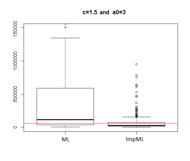
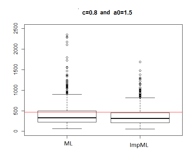
The red line stands stands for the real value of $s_{\alpha}$

Figure 10: Estimations of the $(1-\alpha)-$quantile of two GPD obtained by Maximum Likelihood and by the improved Maximum Likelihood method

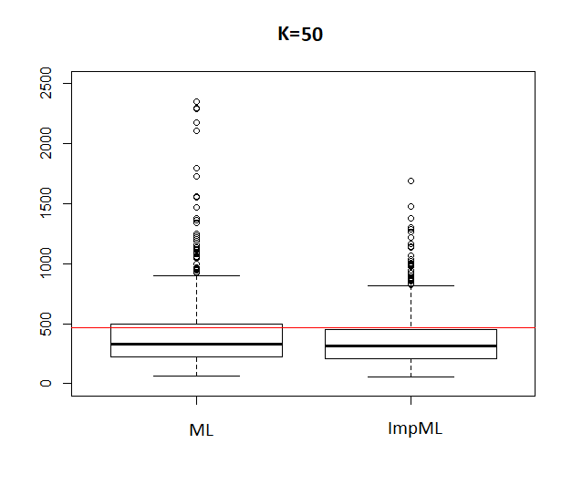
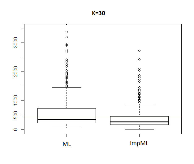
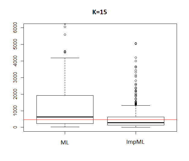
The red line stands stands for the real value of $s_{\alpha}$

Figure 11: Estimations of the $(1-\alpha)-$quantile of a $GPD(0.8,1.5)$ obtained by Maximum Likelihood and by the improved Maximum Likelihood method for different values of $K$.

4.3 Performance of the sequential estimation

As stated in chapter 2, there is to our knowledge no method dealing with similar question available in the literature. Therefore we compare the results of our method, based on observed exceedances over thresholds, with the results that could be obtained by classical extreme quantiles estimation methods assuming we have complete data at our disposal; those may be seen as benchmarks for an upper bound of the performance of our method.

4.3.1 Estimation of an extreme quantile based on complete data, de Valk’s estimator

In order to provide an upper bound for the performance of the estimator, we make use of the estimator proposed by De Valk and Cai (2016). This work aims at the estimation of a quantile of order $p_{n}\in[n^{-\tau_{1}};n^{-\tau_{2}}]$, with $\tau_{2}>\tau_{1}>1$ , where $n$ is the sample size. This question is in accordance with the industrial context which motivated the present paper. De Valk’s proposal is a modified Hill estimator adapted to log-Weibull tailed models. De Valk’s estimator is consistent, asymptotically normally distributed, but is biased for finite sample size.We briefly recall some of the hypotheses which set the context of de Valk’s approach.

Let $X_{1},\dots,X_{n}$ be $n$ iid r.v’s with distribution $F$, and denote $X_{k:n}$ the $k-$ order statistics. A tail regularity assumption is needed in order to estimate a quantile with order greater than $1-$ $1/n.$

Denote $U(t)=F^{-1}\left(1-1/t\right)$, and let the function $q$ be defined by

$$q(y)=U(e^{y})=F^{-1}\left(1-e^{-y}\right)$$

for $y>0$.

Assume that

$$\lim\limits_{y\rightarrow\infty}~{}\frac{\log q(y\lambda)-\log q(y)}{g(y)}=h_{\theta}(\lambda)~{}~{}~{}\lambda>0$$ (14)

where $g$ is a regularly varying function and

$$h_{\theta}(\lambda)=\left\{\begin{array}[]{l}\frac{\lambda^{\theta}-1}{\theta}\text{ if }\theta\neq 0\\ \log\lambda\text{ if }\theta=0\end{array}\right.$$

de Valk writes condition 14 as $\log q\in ERV_{\theta}(g)$.

Remark : Despite its naming of log-Generalized tails, this condition also holds for Pareto tailed distributions, as can be checked, providing $\theta=1.$

We now introduce de Valk’s extreme quantile estimator.

Let

$$\vartheta_{k,n}:=\sum_{j=k}^{n}\frac{1}{j}.$$

Let $q(z)$ be the quantile of order $e^{-z}=p_{n}$ of the distribution $F$. The estimator makes use of $X_{n-l_{n}:n}$, an intermediate order statistics of $X_{1},..,X_{n}$, where $l_{n}$ tends to infinity  as $n\rightarrow\infty$ and $l_{n}$ $\ /n\rightarrow 0.$

de Valk’s estimator writes

$$\widehat{q}(z)=X_{n-l_{n}:n}\exp\left\{g(\vartheta_{l_{n},n})h_{\theta}\left(\frac{z}{\vartheta_{l_{n+1},n}}\right)\right\}.$$ (15)

When the support of $F$ overlaps $\mathbb{R}^{-}$ then the sample size $n$ should be large; see de Valk ([8]) for details.

Note that, in the case of a $GPD(c,a)$, parameter $\theta$ is known and equal to 1 and the normalizing function $g$ is defined by $g(x)=cx$ for $x>0$.

4.3.2 Loss in accurracy due to binary sampling

In Table 7 we compare the performance of de Valk’s method with ours on the model, making use of complete data in de Valk’s estimation, and of dichotomous ones in our approach. Clearly de Valk’s results cannot be attained by the present sequential method, due to the loss of information induced by thresholding and dichotomy. Despite this, the results can be compared, since even if the bias of the estimator clearly exceeds the corresponding bias of de Valk’s, its dispersion is of the same order of magnitude, when handling heavy tailed GPD models. Note also that given the binary nature of the data considered, the average relative error is quite honorable. We can assess that a large part of the volatility of the estimator produced by our sequential methodology is due to the nature of the GPD model as well as to the sample size.

	Relative error on the $(1-\alpha)-$quantile
Parameters	On complete data		On binary data
	Mean	Std	Mean	Std
$c=0.8$, $a_{0}=1.5$ and $s_{\alpha}=469.103$	0.052	0.257	-0.222	0.554
$c=1.5$, $a_{0}=1.5$ and $s_{\alpha}=31621.777$	0.086	0.530	-0.504	0.720
$c=1.5$, $a_{0}=3$ and $s_{\alpha}=63243.550$	0.116	0.625	0.310	0.590

Table 7: Mean and std of the relative errors on the $1-\alpha-$quantile of GPD on complete and binary data for samples of size $n=250$ computed through $400$ replicas of both estimation procedures.
Estimations on complete data are obtained with de Valk’s method; estimations on binary data are provided by the sequential design.

5 Sequential design for the Weibull model

The main property which led to the GPD model is the stability through threshold conditioning. However the conditional distribution of $\widetilde{R}$ given $\left\{\widetilde{R}>s\right\}$ takes a rather simple form which allows for some variation of the sequential design method.

5.1 The Weibull model

Denote $\widetilde{R}\sim W(\alpha,\beta)$, with $\alpha,\beta>0$ a Weibull r.v. with scale parameter $\alpha$ and shape parameter $\beta.$ let $G$ denote the distribution function of $\widetilde{R}$ , $g$ its density function and $G^{-1}$ its quantile function. We thus write for non negative $x$

$$\begin{split}~{}G(x)&=1-\exp\left(-\left(\frac{x}{\alpha}\right)^{\beta}\right)\\ \text{ for }0<u<1,~{}~{}G^{-1}(u)&=\alpha(-\log(1-u))^{1/\beta}\end{split}$$

The conditional distribution of $\widetilde{R}$ is a truncated Weibull distribution

$$\begin{split}\text{ for }\widetilde{s}_{2}>\widetilde{s}_{1},~{}~{}\mathbb{P}(\widetilde{R}>\widetilde{s}_{2}\mid\widetilde{R}>\widetilde{s}_{1})&=\frac{\mathbb{P}(\widetilde{R}>\widetilde{s}_{2})}{\mathbb{P}(\widetilde{R}>\widetilde{s}_{1})}\\ &=\exp\left\{\left(-\left(\frac{s_{2}}{\alpha}\right)^{\beta}+\left(\frac{s_{1}}{\alpha}\right)^{\beta}\right)\right\}\end{split}$$

Denote $G_{s_{2}}$ the distribution function of $\widetilde{R}$ given $\left(\widetilde{R}>\widetilde{s}_{2}\right)$.

The following result helps. For $\widetilde{s}_{2}>\widetilde{s}_{1}$,

$$\log\mathbb{P}(\widetilde{R}>\widetilde{s}_{2}\mid\widetilde{R}>\widetilde{s}_{1})=\left[\left(\frac{\widetilde{s}_{2}}{\widetilde{s}_{1}}\right)^{\beta}-1\right]\log\mathbb{P}(\widetilde{R}>\widetilde{s}_{1})$$ (16)

Assuming $\mathbb{P}(\widetilde{R}>\widetilde{s}_{1})=p$, and given $\widetilde{s}_{1}$ we may find $\widetilde{s}_{2}$ the conditional quantile of order $1-p$ of the distribution of $\widetilde{R}$ given $\left\{\widetilde{R}>\widetilde{s}_{1}\right\}$. This solves the first iteration of the sequential estimation procedure through

$$\log p=\left[\left(\frac{\widetilde{s}_{2}}{\widetilde{s}_{1}}\right)^{\beta}-1\right]\log p$$

where the parameter $\beta$ has to be estimated on the first run of trials.

The same type of transitions holds for the iterative procedure; indeed for $\widetilde{s}_{j+1}>\widetilde{s}_{j}>\widetilde{s}_{j-1}$

$$\begin{split}\log\mathbb{P}(\widetilde{R}>\widetilde{s}_{j+1}\mid\widetilde{R}>\widetilde{s}_{j})&=\left[\frac{\log\mathbb{P}(\widetilde{R}>\widetilde{s}_{j+1}\mid\widetilde{R}>\widetilde{s}_{j-1})}{\log\mathbb{P}(\widetilde{R}>\widetilde{s}_{j}\mid\widetilde{R}>\widetilde{s}_{j-1})}-1\right]\log\mathbb{P}(\widetilde{R}>\widetilde{s}_{j}\mid\widetilde{R}>\widetilde{s}_{j-1})\\ &=\left[\frac{\widetilde{s}_{j-1}^{\beta}-\widetilde{s}_{j+1}^{\beta}}{\widetilde{s}_{j-1}^{\beta}-\widetilde{s}_{j}^{\beta}}-1\right]\log\mathbb{P}(\widetilde{R}>\widetilde{s}_{j}\mid\widetilde{R}>\widetilde{s}_{j-1})\end{split}$$ (17)

At iteration $j$ the thresholds $\widetilde{s}_{j}$ and $\widetilde{s}_{j-1}$ are known; the threshold $\widetilde{s}_{j+1}$ is the $(1-p)-$ quantile of the conditional distribution, $\mathbb{P}(\widetilde{R}>\widetilde{s}_{j+1}\mid\widetilde{R}>\widetilde{s}_{j})=p$, hence solving

$$\log p=\left[\frac{\widetilde{s}_{j-1}^{\beta}-\widetilde{s}_{j+1}^{\beta}}{\widetilde{s}_{j-1}^{\beta}-\widetilde{s}_{j}^{\beta}}-1\right]\log p$$

where the estimate of $\beta$ is updated from the data collected at iteration $j.$

5.2 Numerical results

Similarly as in Sections 4.2 and 4.3 we explore the performance of the sequential design estimation on the Weibull model. We estimate the $(1-\alpha)-$ quantile of the Weibull distribution in three cases. In the first one, the scale parameter $a$ and the shape parameter $b$ satisfy $\left(a,b\right)=\left(3,0.9\right)$. This corresponds to a strictly decreasing density function, with heavy tail. In the second case, the distribution is skewed since $\left(a,b\right)=\left(3,1.5\right)$ and the third case is $\left(a,b\right)=\left(2,1.5\right)$ and describes a less dispersed distribution with lighter tail.

Table 8 shows that the performance of our procedure here again depends on the shape of the distribution. The estimators are less accurate in case 1, corresponding to a heavier tail. Those results are compared to the estimation errors on complete data through de Valk’s methodology. As expected, the loss of accuracy linked to data deterioration is similar to what was observed under the Pareto model, although a little more important. This can be explained by the fact that the Weibull distribution is less adapted to the splitting structure than the GPD.

	Relative error on the $(1-\alpha)-$quantile
Parameters	On binary data		On complete data
	Mean	Std	Mean	Std
$a_{0}=3$, $b_{0}=0.9$ et $s_{\alpha}=25.69$	0.282	0.520	0.127	0.197
$a_{0}=3$, $b_{0}=1.5$ et $s_{\alpha}=10.88$	-0.260	0.490	0.084	0.122
$a_{0}=2$, $b_{0}=1.5$ et $s_{\alpha}=7.25$	-0.241	0.450	0.088	0.140

Table 8: Mean and std of relative errors on the $(1-\alpha)-$quantile of Weibull distributions on complete and binary data for samples of size $n=250$ computed through $400$ replicas.
Estimations on complete data are obtained with de Valk’s method; estimations on binary data are provided by the sequential design.

6 Model selection and misspecification

In the above sections, we considered two models whose presentation was mainly motivated by theoretical properties. As it has already been stated in paragraph 3.3, the modeling of $\widetilde{R}$ by a GPD with $c$ strictly positive is justified by the assumption that the support of the original variable $R$ may be bounded by 0. However, note that the GPD model can be easily extended to the case where $c=0$. It then becomes the trivial case of the estimation of an exponential distribution.

Though we did exclude the exponential case while modeling the excess probabilities of $\widetilde{R}$ by a GPD, we still considered the Weibull model in section 5, which belongs to the max domain of attraction for $c=0$. On top of being exploitable in the splitting structure, the Weibull distribution is a classical tool when modeling reliability issues, it thus seemed natural to propose an adaptation of the sequential method for it.

In this section, we discuss the modeling decisions and give some hints on how to deal with misspecification.

6.1 Model selection

The decision between the Pareto model with tail index strictly positive and the Weibull model has been covered in the literature. There exists a variety of tests on the domain of attraction of a distribution.

Dietrich and al. (2002 [9]) Drees and al. (2006 [12]) both propose a test for extreme value conditions related to Cramer-von Mises tests. Let $X$ of distribution function $G$. The null hypothesis is

$$H_{O}:G\in MDA(c_{0}).$$

In our case, the theoretical value for the tail index is $c_{0}=0$. The former test provides a testing procedure based on the tail empirical quantile function, while the latter uses a weighted approximation of the tail empirical distribution. Choulakian and Stephens (2001 [4]) proposes a goodness of fit test in the fashion of Cramer-von Mises tests in which the unknown parameters are replaced by maximum likelihood estimators. The test consists in two steps: firstly the estimation of the unknown parameters, and secondly the computation of the Cramer-von Mises $W^{2}$ or Anderson-Darling $A^{2}$ statistics. Let $X_{1},\dots,X_{n}$ be a random sample of distribution $G$. The hypothesis to be tested is: $H_{O}$: The sample is coming from a $GPD(c_{0},\widehat{a})$. The associated test statistics are given by:

$$\begin{split}&W^{2}=\sum_{i=1}^{n}\left(\widehat{G}(x_{(i)})-\frac{2i-1}{2n}\right)^{2}+\frac{1}{12n};\\ &A^{2}=-n-\frac{1}{n}\sum_{i=1}^{n}(2i-1)\left\{\log(\widehat{G}(x_{(i)}))+\log(1-\widehat{G}(x_{(}n+1-i))\right\},\end{split}$$

where $x_{(i)}$ denotes the $i-$th order statistic of the sample. The authors provide the corresponding tables of critical points.

Jurečková and Picek (2001 [15]) designed a non-parametric test for determining whether a distribution $G$ is light or heavy tailed. The null hypothesis is defined by :

$$H_{c_{O}}:x^{1/c_{0}}(1-G(x))\leq 1~{}~{}\forall x>x_{0}\text{ for some }x_{0}>0$$

with fixed hypothetical $c_{0}$. The test procedure consists in splitting the data set in $N$ samples and computing the empirical distribution of the extrema of each sample.

The evaluation of the suitability of each model for fatigue data is precarious. The main difficulty here is that it is not possible to perform goodness-of-fit type tests, since firstly, we collect the data sequentially during the procedure and do not have a sample of available observations beforehand, and secondly, we do not observe the variable of interest $R$ but only peaks over chosen thresholds. The existing tests procedures are not compatible with the reliability problem we are dealing with. On the first hand, they assume that the variable of interest is fully observed and are mainly semi-parametric or non-parametric tests based on order statistics. On the other hand, their performances rely on the availability of a large volume of data. This is not possible in the design we consider since fatigue trial are both time consuming and extremely expensive.

Another option consists of validating the model a posteriori, once the procedure is completed using expert advices to confirm or not the results. For that matter, a procedure following the design presented in 3.2 is currently being carried out. Its results should be available in a few months and will give hints on the most relevant model.

6.2 Misspecification

In paragraph 3.3, we assumed that $\widetilde{R}$ initially follows a GPD. In practice, the distribution may have its excess probabilities converge towards it as the thresholds increase but differ from a GPD. In the following, let us assume that $\widetilde{R}$ does not follow a GPD (of distribution function $F$) but another distribution $G$ whose tail gets closer and closer to a GPD.

In this case, the issue is to control the distance between $G$ and the theoretical GPD and to determine from which thresholding level it becomes negligible. One way to deal with this problem is to restrict the model to a class of distributions that are not so distant from $F$: Assume that the distribution function $G$ of the variable of interest $\widetilde{R}$ belongs to a neighborhood of the $GPD(c,a)$ of distribution function $F$, defined by:

$$V_{\epsilon}(F)=\left\{G:\sup_{x}|\bar{F}(x)-\bar{G}(x)|w(x)\leq\epsilon\right\},$$ (18)

where $\epsilon\geq 0$ and $w$ an increasing weight function such that $\lim_{x\rightarrow\infty}w(x)=\infty$.

$V_{\epsilon}(F)$ defines a neighborhood which does not tolerate large departures from $F$ in the right tail of the distribution.

Let $x\geq s$, it follows from (18) a bound for the conditional probability of $x$ given $R>s$:

$$\frac{\bar{F}(x)-\epsilon/w(x)}{\bar{F}(s)+\epsilon/w(s)}\leq\frac{\bar{G}(x)}{\bar{G}(s)}\leq\frac{\bar{F}(x+)+\epsilon/w(x)}{\bar{F}(s)-\epsilon/w(s)}.$$ (19)

When $\epsilon=0$, the bounds of (19) match the conditional probabilities of the theoretical Pareto distribution.

In order to control the distance between $F$ and $G$, the bound above may be rewritten in terms of relative error with respect to the Pareto distribution. Using a Taylor expansion of the right and left bounds when $\epsilon$ is close to 0, it becomes:

$$1-u(s,x).\epsilon\leq\frac{\frac{\bar{G}(x)}{\bar{G}(s)}}{\frac{\bar{F}(x)}{\bar{F}(s)}}\leq 1+u(x,s).\epsilon,$$ (20)

where

$$u(s,x)=\frac{\left(1+\frac{cs}{a}\right)^{1/c}}{w(s)}+\frac{\left(1+\frac{cx}{a}\right)^{1/c}}{w(x)}.$$

For a given $\epsilon$ close to 0, the relative error on the conditional probabilities can be controlled upon $s$. Indeed, then the relative error is bounded by a fixed level $\delta>0$ whenever:

$$\frac{\left(1+\frac{cs}{a}\right)^{1/c}}{w(s)}\leq\frac{\delta}{\epsilon}\frac{\left(1+\frac{cx}{a}\right)^{1/c}}{w(x)}.$$

7 Perspectives, generalization of the two models

In this work, we have considered two models for $\widetilde{R}$ that exploits the thresholding operations used in the splitting method. This is a limit of this procedure as the lack of relevant information provided by the trials do not enable a flexible modeling of the distribution of the resistance. In the following, we present ideas of extensions and generalizations of those models, based on common properties of the GPD and Weibull models.

7.1 Variations around mixture forms

When the tail index is positive, the GPD is completely monotone, and thus can be written as the Laplace transform of a probability distribution. Thyrion (1964[21]) and Thorin (1977[20]) established that a $GPD(a_{T},c_{T})$, with $c_{T}>0$, can be written as the Laplace transform of a Gamma r.v $V$ whose parameters are functions of $a_{T}$ and $c_{T}$: $V~{}\sim~{}\Gamma\left(\frac{1}{c_{T}},\frac{a_{T}}{c_{T}}\right)$. Denote $v$ the density of $V$,

$$\begin{split}\forall x\geq 0,~{}~{}\bar{G}(x)=&\int_{0}^{\infty}\exp(-xy)v(y)dy\\ &\text{ where }~{}~{}v(y)=\frac{(a_{T}/c_{T})^{1/c}}{\Gamma(1/c_{T})}y^{1/c_{T}-1}\exp\left(-\frac{a_{T}y}{c_{T}}\right).\end{split}$$ (21)

It follows that the conditional survival function of $\widetilde{R}$, $\bar{G}_{s_{j}}$, is given by:

$$\mathbb{P}(\widetilde{R}>\widetilde{s}_{j+1}\mid\widetilde{R}_{j}>\widetilde{s}_{j}) =\bar{G}_{\widetilde{s}_{j}}(\widetilde{s}_{j+1}-\widetilde{s}_{j})$$

$$=\int_{0}^{\infty}\exp\left\{-(\widetilde{s}_{j+1}-\widetilde{s}_{j})y\right\}v_{j}(y)dy,$$

$$\text{ ~{}~{}where }V_{j}\text{ is a r.v of distribution }\Gamma\left(\frac{1}{c_{j}},\frac{a_{j}}{c_{j}}\right).$$

with $c_{j}=c_{T}$ and $a_{j}=a_{j-1}+c_{T}(\widetilde{s}_{j}-\widetilde{s}_{j-1})$.

Expression (21) gives room to an extension of the Pareto model. Indeed, we could consider distributions of $\widetilde{R}$ that share the same mixture form with a mixing variable $W$ that possesses some common characteristics with the Gamma distributed r.v. $V.$

Similarly, the Weibull distribution $W(\alpha,\beta)$ can also be written as the Laplace transform of a stable law of density $g$ whenever $\beta\leq 1$. Indeed, it holds from Feller 1971[14]) (p. 450, Theorem 1) that:

$$\forall x\geq 0,~{}~{}\exp\left\{-x^{\beta}\right\}=\int_{0}^{\infty}\exp(-xy)g(y)dy$$ (22)

where $g$ is the density of an infinitely divisible probability distribution.

It follows, for $s_{j}<s_{j+1}$

$$\begin{split}\mathbb{P}(\widetilde{R}>\widetilde{s}_{j+1}\mid\widetilde{R}_{j}>\widetilde{s}_{j})&=\frac{\exp\left\{-(\widetilde{s}_{j+1}/\alpha)^{\beta}\right\}}{\exp\left\{-(\widetilde{s}_{j}/\alpha)^{\beta}\right\}}\\ &=\frac{\int_{0}^{\infty}\exp\left\{(-(\widetilde{s}_{j+1}/\alpha)y\right\}g(y)dy}{\int_{0}^{\infty}\exp\left\{-(\widetilde{s}_{j}/\alpha)y\right\}g(y)dy}=\frac{\int_{0}^{\infty}\exp\left\{-(\widetilde{s}_{j+1}/\alpha)y\right\}g(y)dy}{K(s_{j})}\\ &=\frac{1}{K(s_{j})}\int_{0}^{\infty}\exp\left\{-\widetilde{s}_{j+1}u\right\}g_{\alpha}(u))du\\ &\quad\quad\text{ with }u=y/\alpha\text{ and }g_{\alpha}(u)=\alpha g(\alpha u)\end{split}$$ (23)

Thus an alternative modeling of $\widetilde{R}$ could consist in any distribution that can be written as a Laplace transform of a stable law of density $w_{\alpha,\beta}$ defined on $\mathbb{R}_{+}$ and parametrized by $(\alpha,\beta)$, that complies to the following condition: For any $s>0$, the distribution function of the conditional distribution of $\widetilde{R}$ given $\widetilde{R}>s$ can be written as the Laplace transform of $w_{\alpha,\beta}^{(\alpha,s)}(.)$ where

$$x>s,w_{\alpha,\beta}^{(\alpha,s)}(x)=\frac{\alpha w_{\alpha,\beta}(\alpha x)}{K(s)},$$

where $K(.)$ is defined in (23).

7.2 Variation around the GPD

Another approach, inspired by Naveau et al. (2016[17]), consists in modifying the model so that the distribution of $\widetilde{R}$ tends to a GPD as $x$ tends to infinity and it takes a more flexible form near 0.

$\widetilde{R}$ is generated through $G_{(c_{T},a_{T})}^{-1}(U)$ with $U\sim\mathcal{U}[0,1]$. Let us consider now a deformation of the uniform variable $V=L^{-1}(U)$ defined on $[0,1]$, and the transform $W$ of the GPD: $W^{-1}(U)=G_{(c_{T},a_{T})}^{-1}(L^{-1}(U))$.

The survival function of the GPD being completely monotone, we can choose $W$ so that the distribution of $\widetilde{R}$ keeps this property.

Proposition 3.

If $\phi:[0,\infty[\rightarrow\mathbb{R}$ is completely monotone and let $\psi$ be a positive function, such that its derivative is completely monotone, then $\phi(\psi)$ est completely monotone.

The transformation of the GPD has cumulative distribution function $W=L(G_{(}c_{T},a_{T}))$ and survival function $\bar{W}=\bar{L}(G_{(}c_{T},a_{T}))$. $G(c_{T},a_{T})$ is a Berstein function, thus $\bar{W}$ is completely monotone if $\bar{L}$ is also.

7.2.1 Examples of admissible functions:

(1) Exponential form :

$$\begin{split}&L(0)=0\\ &L(x)=\frac{1-\exp(-\lambda x^{\alpha})}{1-\exp(-\lambda)}~{}~{}~{}\text{avec }0\leq\alpha\leq 1\text{ et }\lambda>0\\ &L(1)=1\end{split}$$

The obtained transformation is: $\forall x>0$,

$$\bar{W}_{(\lambda,c_{T},a_{T})}(x)=\bar{L}(G(x))=\frac{\exp\left(-\lambda\left[1-(1+\frac{c_{T}}{a_{T}})^{-1/c_{T}}\right]^{\alpha}\right)-\exp(-\lambda)}{1-\exp(-\lambda)}$$

with $\bar{W}_{(\lambda,c_{T},a_{T})}(x)$ completely monotone.

(2) Logarithmic form:

$$\begin{split}&L(0)=0\\ &L(x)=\frac{\log(x+1)}{\log 2}~{}~{}~{}~{}\text{ \big{(} or more generally }\frac{\log(\alpha x+1)}{\log 2},~{}\alpha>0\text{\big{)}}\\ &L(1)=1\end{split}$$

and $\forall x>0$,

$$\bar{W}_{(c_{T},a_{T})}(x)=1-\frac{\log\left(2-(1+\frac{c_{T}}{a_{T}})^{-1/c_{T}}\right)}{\log 2}$$

(3) Root form:

$$\begin{split}&L(0)=0\\ &L(x)=\frac{\sqrt{x+1}-1}{\sqrt{2}-1}\\ &L(1)=1\end{split}$$

and

$$\bar{W}_{(c_{T},a_{T})}x)=1-\frac{\sqrt{2-(1+\frac{c_{T}x}{a_{T}})^{-1/c_{T}}}-1}{\sqrt{2}}$$

(4) Fraction form:

$$\begin{split}&L(0)=0\\ &L(x)=\frac{(\alpha+1)x}{x+\alpha},~{}~{}\alpha>0\\ &L(1)=1\end{split}$$

and

$$\bar{W}_{(\alpha,c_{T},a_{T})}(x)=1-\frac{(\alpha+1)\left(1-(1+\frac{c_{T}x}{a_{T}})^{-1/c}\right)}{1-(1+\frac{c_{T}x}{a_{T}})^{-1/c_{T}}+\alpha}$$

The shapes of the above transformations of the GPD are shown in Figure 12.

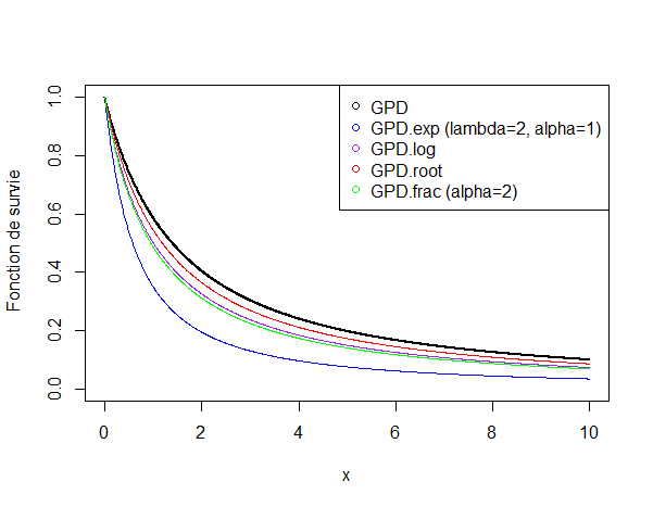
Figure 12: Survival functions associated with transformations of the GPD$(0.8,1.5)$

However those transformations do not conserve the stability through thresholding of the Pareto distribution. Thus, their implementation does not give stable results. Still they give some insight on a simple generalization of the proposed models usable under additional information on the variable of interest.

8 Conclusion

The splitting induced procedure presented in this article proposes an innovative experimental plan to estimate an extreme quantile. Its development has been motivated by on the one hand major industrial stakes, and on the other hand the lack of relevance of existing methodologies. The main difficulty in this setting is the nature of the information at hand, since the variable of interest is latent, therefore only peaks over thresholds may be observed. Indeed, this study is directly driven from an application in material fatigue strength: when performing a fatigue trial, the strength of the specimen obviously can not be observed; only the indicator of whether or not the strength was greater than the tested level is available.

Among the methodologies dealing with such a framework, none is adapted to the estimation of extreme quantiles. We therefore proposed a plan based on splitting methods in order to decompose the initial problem into less complex ones. The splitting formula introduces a formal decomposition which has been adapted into a practical sampling strategy targeting progressively the tail of the distribution of interest.

The structure of the splitting equation has motivated the parametric hypothesis on the distribution of the variable of interest. Two models exploiting a stability property have been presented: one assuming a Generalized Pareto Distribution and the other a Weibull distribution.

The associated estimation procedure has been designed to use the iterative and stable structure of the model by combining a classical maximum likelihood criterion with a consistency criterion on the sequentially estimated quantiles. The quality of the estimates obtained through this procedure have been evaluated numerically. Though constrained by the quantity and quality of information, those results can still be compared to what would be obtained ideally if the variable of interest was observed.

On a practical note, while the GPD is the most adapted to the splitting structure, the Weibull distribution has the benefit of being particularly suitable for reliability issues. The experimental campaign launched to validate the method will contribute to select a model.

References

- [1] Balkema A. A. and De Haan L.: Residual Life Time at Great Age. Ann. Prob., vol. 2 (5) pp. 762 - 804 (1974).
- [2] Beirlant J., Guillou A. and Dierckx G. and Fils-Villetard A.: Estimation of the extreme value index and extreme quantiles under random censoring. Extremes, vol. 10 (3) pp. 151 - 174 (2007).
- [3] Biret M. and Broniatowski M.: SAFIP: a streaming algorithm for inverse problems. arXiv (2016).
- [4] Choulakian, V., Stephens, M. A.: Goodness-of-fit tests for the generalized Pareto distribution. Technometrics 43(4), 4978–484 (2001)
- [5] De Haan L. and Rootzén H.: On the estimation of high quantiles. J. Statist. Plann. Inference, vol. 35 (1) pp. 1 - 13 (1993).
- [6] Dekkers A.L.M., Einmahl J. H. J. and De Haan L.: A moment estimator for the index of an extreme-value distribution. Ann. Statist., vol. 17 (4) pp. 1833—1855 (1989).
- [7] De Valk C.: Approximation of high quantiles from intermediate quantiles. Extremes, vol. 4 pp. 661 - 684 (2016).
- [8] De Valk C. and Cai J.J: A high quantile estimator based on the log-Generalised Weibull tail limit. Econometrics and Statistics, vol. 6 pp. 107 - 128 (2018).
- [9] Dietrich, D., De Haan, L. and Hüsler, J.: Testing extreme value conditions. Extremes 5(1), 71–85 (2002).
- [10] Dixon W. J. and Mood A. M.: A Method for Obtaining and Analyzing Sensitivity Data. Journal of the American Statistical Association, vol. 43 pp. 109 - 126 (1948).
- [11] Dixon W. J.: The Up-and-Down Method for Small Samples. Journal of the American Statistical Association, vol. 60 pp. 967 - 978 (1965).
- [12] Drees, H., De Haan, L. and Li, D.: Approximations to the tail empirical distribution function with application to testing extreme valueconditions. J. Statist. Plann. Inference 136(10), 3498–3538 (2006).
- [13] Einmahl J.H.J, Fils-Villetard A. and Guillou A. Statistics of extremes under random censoring, Bernoulli, vol 14(1) pp. 207–227 (2008)
- [14] Feller W.: An introduction to probability theory and its applications. Wiley, vol 2 (1971)
- [15] Jurečková, J. and Picek, J.: A Class of Tests on the Tail Index. Extremes, 4, 165 – 183 (2001).
- [16] Kahn, H. and E Harris, T.: Estimation of Particle Transmission by Random Sampling. National Bureau of Standards Applied Mathematics Series, vol. 12 (1951).
- [17] Naveau, P.; Huser, R.; Ribereau, P. and Hannart A.: Modeling jointly low, moderate, and heavy rainfall intensities without a threshold selection. Water Resources Research, vol. 52 (4) pp. 2753 - 2769 (2016).
- [18] O’Quigley J. and Pepe M. and Fisher L.l.: Continual Reassessment Method: A Practical Design for Phase 1 Clinical Trials in Cancer. Biometrics, vol. 46 pp. 33 - 48 (1990).
- [19] Pickands J.: Statistical Inference using extreme order statistics. Ann. Prob., vol. 3 (1) pp. 119 - 131 (1975).
- [20] Thorin O.: On the infinite divisibility of the Pareto distribution. Scand. Actuarial J., vol. 1 pp. 31 - 40 (1977).
- [21] Thyrion P.: Les lois exponentielles composées. Bulletin de l’Association Royale des Actuaires Belges, vol. 62 pp. 35 - 44 (1964).
- [22] Weissman, I.:Estimation of parameters and large quantiles based on the k largest observations. J. Amer. Statist. Assoc., vol. 73 pp. 812 - 815 (1978).
- [23] Worms J. and Worms R.: New estimators of the extreme value index under random right censoring, for heavy-tailed distributions. Extremes, vol. 17 pp. 337 - 358 (2014).