Klein Bound States in Single-Layer Graphene

Abstract

The Klein paradox, first introduced in relation to chiral tunneling, is also manifested in the study of bound-states in single-layer graphene with a 1D square-well potential. We derive analytic (and numerical) solutions for bound-state wavefunctions, in the absence and in the presence of an external transverse magnetic field, and calculate the corresponding dipole transition rates, which can be probed by photon absorption experiments. The role of parity and time-reversal symmetries is briefly discussed. Our results are also relevant for the physics of bound states of light in periodic optical waveguide structures.

Introduction.— Chiral tunneling of electrons through a 1D potential barrier in single layer graphene was first considered in a seminal paper by Katsnelson, Novoselov, and Geim Katsnelson_06 . A closely related and physically motivated problem concerns the formation of electron bound states in a 1D (symmetric) potential well Peeters ; Barbier ; Ramezani ; Nguyen_09 ; Gutierrez_16 (bound-states here refers to bound in one direction and free in the other direction). In this Letter we elucidate several novel aspects of such bound-states amenable to experimental verification. Our main results are: (1) In the absence of a magnetic field, bound-state eigenfunctions and eigenvalues are derived analytically, and electric dipole transition strengths are calculated to determine the absorption spectrum between bound-states. Parity and time reversal symmetry are employed to find the relation between the two (pseudo)-spinor components. (2) In the presence of an external magnetic field, analytic expressions for the bound state wavefunctions for a discrete sequence of potential strengths are derived, and are used to determine the measurable areal densities and currents. Based on ideas presented in Refs. Longhi_10 ; Longhi_11 , our formalism also applies to the occurrence of bound states of light in periodic optical waveguide structures.

Bound states in a symmetric 1D square-well.— We search for bound states of a massless particle in single-layer graphene using the 2D Dirac equation with 1D square-well symmetric potential $U(x)=U_{0}\Theta(|x|-L)$. Employing $L$ as a length unit, we define dimensionless coordinates $x\to x/L,\ \ y\to y/L$, potential $u(x)=LU(x)/(\hbar v_{F})\equiv u_{0}\Theta(|x|-1)$, energy $\varepsilon=LE/(\hbar v_{F})$, (where $E$ is the energy in physical units), and wavenumber $k=\varepsilon$, (where $E/(\hbar v_{F})$ is the Fermi wavenumber in physical units). Klein physics Klein occurs for $u_{0}>\varepsilon>0$ where inside the well ($|x|<1$) the Fermi energy lies in the conduction band while outside the well ($|x|>1$) the Fermi energy lies in the valence band Klein ; AF_11 . Near the ${\bf K}^{\prime}$ Dirac point, the time-independent 2D Dirac equation (in dimensionless variables) is,

$${\cal H}\Psi\equiv[-i(\sigma_{x}\partial_{x}+\sigma_{y}\partial_{y})+u(x)]\Psi(x,y)=\varepsilon\Psi(x,y).$$ (1)

Under parity transformation $(x,y)\to(-x,y)$, the potential is symmetric, $u(x)=u(-x)$, but the total Hamiltonian is not, ${\cal H}(-x,y)\neq{\cal H}(x,y)$. The general solution of the wavefunction in the three different regions is, $\Psi(x,y)=e^{ik_{y}y}\psi(x)$,

$$\psi(x)\mbox{=}\begin{cases}a\binom{1}{e^{i\phi}}e^{ik_{x}x}+b\binom{1}{-e^{-i\phi}}e^{-ik_{x}x}\ \ (|x|<1),\\ \alpha\binom{1}{-e^{i\theta}}e^{iq_{x}x}+\beta\binom{1}{e^{-i\theta}}e^{-iq_{x}x}\ \ (x>1),\\ \gamma\binom{1}{-e^{i\theta}}e^{iq_{x}x}+\delta\binom{1}{e^{-i\theta}}e^{-iq_{x}x}\ \ (x<-1),\end{cases}$$ (2)

where $\phi$ is the inclination angle and $\theta$ is the refractive angle. The dimensionless momentum vector inside the well [where $u(x)=0$] is

$${\bf k}=\varepsilon(\cos\phi~{}\hat{\bf x}+\sin\phi~{}\hat{\bf y})\equiv k_{x}\hat{\bf x}+k_{y}\hat{\bf y},$$ (3)

and $|{\bf k}|=\varepsilon=\sqrt{k_{x}^{2}+k_{y}^{2}}$. The $x$ component of the momentum outside the well [where $u(x)=u_{0}>0$] and the refractive angle are given by

$$q_{x}=\sqrt{(\varepsilon-u_{0})^{2}-k_{y}^{2}},$$

$$\tan\theta=\frac{k_{y}}{q_{x}}=\frac{\varepsilon\sin\phi}{\sqrt{(\varepsilon-u_{0})^{2}-(\varepsilon\sin\phi)^{2}}}.$$ (4)

In the $p$-$n$-$p$ junction analyzed here, Klein tunneling occurs for $u_{0}/(1+\sin\phi)>\varepsilon>0$ (where $q_{x}$ is real), whereas Klein bound states occur for $u_{0}>\varepsilon>u_{0}/(1+\sin\phi)>0$, for which

$$q_{x}=i\kappa_{x}(\varepsilon,\phi)\equiv i\sqrt{(\varepsilon\sin\phi)^{2}-(u_{0}-\varepsilon)^{2}},$$ (5)

and $\kappa_{x}(\varepsilon,\phi)>0$. The bound state wavefunctions must decay exponentially as $e^{-\kappa_{x}|x|}$ as $|x|\to\infty$. In this region $\tan\theta=-ik_{y}/\kappa_{x}$ is pure imaginary, and $\tan^{2}\theta<-1$. Consequently, $\sin\theta$ is real and $\cos\theta$ is imaginary. To insure asymptotic decay at large $|x|$ we must set $\beta=\gamma=0$ in Eq. (2). Continuity of $\psi(x)$ at $x=\pm 1$ yields a homogeneous system of four linear equations for the complex coefficient vector ${\bf c}\equiv(a,b,\alpha,\delta)^{T}$ that is an eigenvector with zero eigenvalue of the matrix $A(\varepsilon)$, $A(\varepsilon){\bf c}=0$ ($A(\varepsilon)$ is explicitly given in the Supplemental Material (SM) SM ). The determinant of $A(\varepsilon)$ is given by

$$C\,\mbox{det}[A(\varepsilon)]=\kappa_{x}(\varepsilon,\phi)\cos\phi\cos(2\varepsilon\cos\phi)$$

$$+[\varepsilon(1+\sin^{2}\phi)-u_{0}]\sin(2\varepsilon\cos\phi),$$ (6)

where $C$ is a non-vanishing multiplicative constant and the expression on the RHS is real. Bound-states occur at energies $\varepsilon_{n}$ for which $\mbox{det}[A(\varepsilon_{n})]=0$. For reasons that will be explained later, we focus on bound states at different energies $\{\varepsilon_{n}\}$ but for the same $k_{y}=\varepsilon_{n}\sin\phi_{n}$. We use the following realistic values for the parameters of graphene: $L=172$ nm, $U_{0}=50$ meV, which yields $u_{0}=\frac{LU_{0}}{\hbar v_{F}}\approx 16.0$. The pattern of bound state energies in the $(\phi,\varepsilon)$ plane is shown in Fig. 1(a), together with the curve $k_{y}=\varepsilon\sin\phi=10$ (= 0.0581 nm^-1). The intersection points indicate bound-state energies $\{\varepsilon_{n}\}$ with the same value of $k_{y}=\varepsilon_{n}\sin\phi_{n}$.

Bound state wavefunctions.— Now we compute the wavefunctions for $(\varepsilon_{n},\phi_{n})$, $n=0,1,\ldots,7$, see Fig. 1(a). The pairs $(\varepsilon_{n},\phi_{n})$ are inserted into the matrix $A$ and the spinor bound-state wavefunctions $\psi_{n}(x)=\binom{\psi_{n}^{(1)}}{\psi_{n}^{(2)}}$ are determined in terms of the four coefficients ${\bf c}_{n}\equiv(a_{n},b_{n},\alpha_{n},\delta_{n})$, i.e., the solution of the eigenvalue equation $A(\varepsilon_{n},\phi_{n}){\bf c}_{n}^{T}=0$. Due to parity symmetry (see below), the components of the spinors are subject to the constraints,

$$\mbox{Im}[\psi_{n}^{(1)}(x)]=\mbox{Re}[\psi_{n}^{(2)}(x)]=0,$$

$$\mbox{Im}[\psi_{n}^{(2)}(x)]=(-1)^{n}\mbox{Re}[\psi_{n}^{(1)}(-x)].$$ (7)

Analytic expressions for the ground and excited state wavefunctions are derived by choosing

$$a=b^{*}={\cal A}_{n}e^{i\eta_{n}},\ \ \eta_{n}=(2n+1)\tfrac{\pi}{4}-\tfrac{1}{2}\phi.$$ (8)

where ${\cal A}_{n}$ are real normalization constants and the phase $\eta_{n}$ is chosen to satisfy the symmetries in Eq. (Klein Bound States in Single-Layer Graphene). Combining Eqs. (2) and (8), the bound-state wavefunctions, $\Psi_{n}(x,y)=e^{ik_{y}y}\psi_{n}(x)$ for $|x|<1$ are,

$$\psi_{n}(x,y)=\mathcal{A}_{n}\binom{\psi_{n}^{(1)}(x)}{(-1)^{n}i\psi_{n}^{(1)}(-x)}$$

$$=\mathcal{A}_{n}\binom{\cos[\gamma_{n}^{-}(x)]+\sin[\gamma_{n}^{-}(x)]}{(-1)^{n}i\{\cos[\gamma_{n}^{+}(x)]+\sin[\gamma_{n}^{+}(x)]\}},$$ (9)

$$\gamma_{n}^{\pm}(x)=\tfrac{1}{2}(\phi_{n}\pm 2k_{nx}x),$$

where $k_{nx}=\varepsilon_{n}\cos\phi_{n}$. The decaying parts of the wavefunctions for $|x|>1$ are determined by the coefficients $\beta,\delta$, and the symmetry specified in Eq. (Klein Bound States in Single-Layer Graphene) is fulfilled for all $x$. The two upper components of the spinor wavefunctions $\psi_{n=0,1}(x)$ are shown in Fig. 1(b).

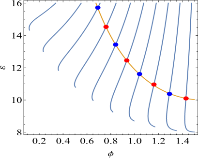
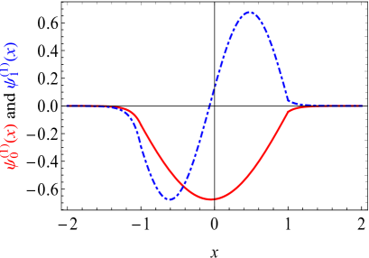
Figure 1: (a) Nodes of det$[A(\varepsilon,\phi)]$, Eq. (Klein Bound States in Single-Layer Graphene), in the $(\phi,\varepsilon)$ plane (blue curves), and the curve $k_{y}=\varepsilon\sin\phi=10$ (orange curve). The pairs $(\varepsilon_{n},\phi_{n})$ specified by blue and red dots are the bound state energies for $k_{y}=\varepsilon_{n}\sin\phi_{n}=10.$ (b) Upper components of $\psi_{0}(x)$ (red solid curve) and $\psi_{1}(x)$ (blue dot-dashed curve) versus $x$. The lower components are related to the upper ones via Eq. (Klein Bound States in Single-Layer Graphene). Note that the wavefunctions do not have a definite symmetry around $x=0$ (see discussion on the role of parity below).

The symmetry specified in Eq. (Klein Bound States in Single-Layer Graphene) also implies that $\psi_{0}^{\dagger}(x)\psi_{1}(x)$ is an odd function of $x$. Hence, $\langle\psi_{0}|\psi_{1}\rangle=0$, i.e., the two states are orthogonal, as are any two different eigenfunctions.

Currents.— Bound states, with wavefunctions $\psi_{n}(x)=\binom{\psi_{n}^{(1)}(x)}{\pm i\psi_{n}^{(1)}(-x)}$, do not carry current along $x$: $J_{nx}(x)\equiv\psi_{n}^{\dagger}(x)\sigma_{x}\psi_{n}(x)=0$. However, they do carry current along $y$, $J_{ny}(x)\equiv\psi_{n}^{\dagger}(x)\sigma_{y}\psi_{n}(x)\neq 0$, $(n=0,1)$, that is symmetric under $x\leftrightarrow-x$ and it quickly decays for $|x|>1$. As we discuss below in connection with time reversal invariance, all states are Kramers degenerate, and the two degenerate states forming a Kramers pair carry currents in opposite directions.

Parity.— The importance of parity in the physics of graphene is discussed in Ref. Riazuddin_18 , where it is shown that parity operator in (1+2) dimensions plays an interesting role and can be used for defining conserved chiral currents (see also Ref. Sadurni_15 ). Here we concentrate on bound states, wherein the current along $x$ should vanish, and consider the role of the parity transformation under which the Hamiltonian is not invariant. For a symmetric potential, $u(x)=u(-x)$, we consider the static (time-independent) case with Hamiltonian ${\cal H}(x,y)$ introduced in Eq. (1). The parity transformation in 2+1 dimensions is taken to mean the transformation $(x,y)\to(-x,y)$. For massless Dirac fermions this transformation is realized by the operator $\sigma_{y}$. Explicitly,

$${\cal H}^{P}(x,y)\equiv\sigma_{y}{\cal H}(x,y)\sigma_{y}=i\sigma_{x}\partial_{x}-i\sigma_{y}\partial_{y}+u(x)$$

$$={\cal H}(-x,y)\neq{\cal H}(x,y).$$ (10)

Thus, near a given Dirac point, say ${\bf K}^{\prime}$, ${\cal H}$ is not parity invariant [despite the fact that $u(x)=u(-x)]$ footnote1 . However, for a symmetric potential the wavefunctions $\psi_{n}(x)$ in Eq. (Klein Bound States in Single-Layer Graphene) obey the symmetry relations,

$$\sigma_{y}\psi_{0}(x)=\psi_{0}(-x),\quad\sigma_{y}\psi_{1}(x)=-\psi_{1}(-x).$$ (11)

Equation (11) is a concrete realization of Eq. (14) in Ref. Riazuddin_18 . Hence, we define $\psi_{n}(x)$ as being $\binom{\text{even}}{\text{odd}}$ under parity if and only if $\sigma_{y}\psi(x)=\pm\psi(-x)$. With this assignment, Eq. (11) is consistent with (albeit different than) the non-relativistic one-dimensional problem, where, in a symmetric potential, the parity of eigenstates is such that $\psi_{n}(-x)=(-1)^{n}\psi_{n}(x),\ n=0,1,2,...$, and the ground-state is symmetric. By definition,

$${\cal H}\psi_{n}(x)=\varepsilon_{n}\psi_{n}(x)\Rightarrow\ {\cal H}^{P}\psi_{n}(-x)=\varepsilon_{n}\psi_{n}(-x).$$ (12)

Thus, $\psi_{n}(x)$ and $\psi_{n}(-x)\neq\pm\psi_{n}(x)$ are respectively eigenfunctions of ${\cal H}$ and ${\cal H}^{P}\neq{\cal H}$ with the same eigenvalue $\varepsilon_{n}$.

Time Reversal Invariance.— The time reversal operator is ${\cal T}=i\sigma_{y}K$, where $K$ is the complex conjugation operator. It is easy to check that $[{\cal H},{\cal T}]=0$, so that each state is doubly (Kramers) degenerate. Applying the operator ${\cal T}$ on a wavefunctions $\Psi_{n}(x,y)$, Eq. (Klein Bound States in Single-Layer Graphene) we obtain [recall that $\psi_{n}^{(1)}(x)$ is real and $\psi_{n}^{(2)}(x)=(-1)^{n}i\psi_{n}^{(1)}(-x)$ is purely imaginary],

$$\Psi_{n}^{\cal T}(x,y)={\cal A}_{n}e^{-ik_{y}y}\binom{(-1)^{n}\psi_{n}^{(1)}(-x)}{i\psi_{n}^{(1)}(x)},$$ (13)

which is the Kramers partner of $\Psi_{n}(x,y)$, i.e., ${\cal H}\Psi_{n}^{\cal T}(x,y)=\varepsilon_{n}\Psi_{n}^{\cal T}(x,y)$.

Electromagnetic Transitions.— Consider $E1$ transitions induced by $x$ polarized light such that the dipole operator is ${\cal O}(x)=eE_{x}x$, where $E_{x}$ is the electric field amplitude. The parity of the product $\psi_{n}^{\dagger}(x)\psi_{m}(x)$ is $(-1)^{n+m+1}$. Because $k_{y}$ is conserved and is the same for $\Psi_{n}(x,y)$ and $\Psi_{m}(x,y)$, we have,

$$\langle\Psi_{m}|{\cal O}|\Psi_{n}\rangle=\tfrac{1}{2}[1-(-1)^{n+m}]eE_{x}\langle x\rangle_{n,m}.$$ (14)

Figure 2 shows the absorption spectrum of the transitions $0\to 1$, $1\to 2$, $0\to 3$, $1\to 4$, $0\to 5$, $1\to 6$, $0\to 7$, where the absorption rates (in arbitrary units) $w_{nm}$ from $m$ to $n$ are proportional to $\omega_{nm}^{4}\,\left|\langle\psi_{n}|x|\psi_{m}\rangle\right|^{2}$ where $\hbar\omega_{nm}=\varepsilon_{n}-\varepsilon_{m}$ Band_Avishai .

Strictly speaking, electrons can occupy orbits with arbitrary $k_{y}<\varepsilon$ and transitions can occur between the pertinent energy states. However, practically, an experiment can be carried out in a graphene nano-ribbon of width $L_{y}$ such that $k_{y}=\frac{2\pi p}{L_{y}},(p=1,2,\ldots)$ is quantized. If $L_{y}$ is small enough, only the lowest mode is occupied. In our example, $k_{y}=10$ and $\varepsilon<u_{0}=16$ (in dimensionless units). If this value of $k_{y}$ corresponds to the lowest mode $p=1$, then the second mode ($p=2$) has $k_{y}=20>\varepsilon$. In physical units, this implies $k_{y}=0.058$ nm^-1 and $L_{y}=108$ nm. Experimental fabrications of much lower nano-ribbon width have already been reported Barone .

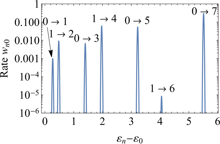
Figure 2: Absorption spectrum of the transitions $0\to 1$, $0\to 3$, $0\to 5$, $0\to 7$, $1\to 2$, $1\to 4$, $1\to 6$. The absorption rate $w_{mn}$ (in dimensionless units) from level $n$ to level $m$ is plotted as a function of the resonant absorption photon energy $\hbar\omega_{nm}=\varepsilon_{n}-\varepsilon_{m}$ (in dimensionless units).

Bound States in a perpendicular magnetic field and square well.— Analysis of bound states in the presence of uniform perpendicular magnetic field and a square well potential enables an access to “un-quantized” Landau functions in graphene. First recall the extensively studied case $U(x)=0$ (see e.g., Ref. Zala ). In the Landau gauge, $A_{y}=Bx$, the spinor wavefunction is $\Psi(x,y)=e^{ik_{y}y}\psi(x)$. Introducing the magnetic length $\ell=\sqrt{\hbar c/(eB)}$ enables formulation in terms of the dimensionless position, wave number and binding energy: $x\to x/\ell$, $k_{x,y}\to k_{x,y}\ell$ and $\varepsilon=\frac{\ell E}{\hbar v_{F}}$. The bare equation with dimensionless variables and parameters then reads, $[-i\sigma_{x}\partial_{x}+\sigma_{y}(k_{y}-x)]\psi(x)=\varepsilon\psi(x)$. It is simplified after a shift and scaling of the position coordinate, $x\to\frac{z}{\sqrt{2}}+k_{y}$,

$${\cal H}\psi(z)\equiv[-i\sigma_{x}\partial_{z}-\tfrac{1}{2}z\sigma_{y}]\psi(z)=\varepsilon\psi(z),$$ (15)

whose general solution is (with $\bar{\delta}\equiv 1-\delta$),

$$\binom{\psi^{(1)}(z)}{\psi^{(2)}(z)}\!=c_{1}\binom{D_{\nu_{1}}(z)}{\tfrac{\varepsilon}{i}D_{\nu_{1}-1}(z)}+c_{2}\bar{\delta}_{\varepsilon,0}\binom{D_{\nu_{2}}(iz)}{\tfrac{-1}{\varepsilon}D_{\nu_{2}+1}(iz)}$$ (16)

where $D_{\nu}(z)$ is the parabolic cylinder function, $z\equiv z(x)=\sqrt{2}(x-k_{y})$, $\nu_{1}=\varepsilon^{2}$, $\nu_{2}=-(\varepsilon^{2}+1)$. If the wavefunction is required to be square integrable on the whole interval $-\infty<z<\infty$, we must set $\varepsilon^{2}=n$, (where $n$ is a non-negative integer), and $c_{2}=0$ (because wavefunctions with imaginary arguments blow up). These constraints determine the Landau quantized energies $\varepsilon=\pm\sqrt{n}$ and wavefunctions for electrons in graphene.

In the scaled shifted variable $z$ the square-well potential $U(x)=U_{0}\Theta(|x|-L)$ reads,

$$u(z)=\begin{cases}0,\ \ z(-L)<z<z(L)\\ u_{0},\ \ \ \ \ \mbox{otherwise}\end{cases},$$ (17)

where $u_{0}=\frac{\ell U_{0}}{\hbar v_{F}}$ and $z(L)=\sqrt{2}L-k_{y}\equiv L_{1}$, $z(-L)=-\sqrt{2}L-k_{y}\equiv L_{2}\neq-z(L)=-L_{1}$, hence $k_{y}=-\frac{1}{2}[z(L)+z(-L)]$. Thus, a symmetric well in $x$ is not symmetric in $z$. The eigenvalue problem is specified by the set of equations defined for $-\infty<z<\infty$,

$$[-i\sigma_{x}\frac{d}{dz}-\tfrac{1}{2}z\sigma_{y}]\psi(z)=\begin{cases}\varepsilon\psi(z),\ \ z\in[L_{2},L_{1}]\\ (\varepsilon-u_{0})\psi(z),\ \ z\notin[L_{2},L_{1}].\end{cases}$$ (18)

Here $\psi(z)=\binom{\psi^{(1)}(z)}{\psi^{(2)}(z)}$, and $\varepsilon$ is the energy eigenvalue that needs to be determined. As in Eq. (16), the solutions can be expressed in terms of parabolic cylinder functions $D_{\nu}(\cdot)$, and the spinor wavefunction is required to be continuous everywhere and square-integrable. For $z\in[L_{2},L_{1}]$ the solution reads,

$$\psi_{\text{c}}(z)=c_{1}\begin{pmatrix}\!D_{\nu_{1}}(z)\\ -i\varepsilon D_{\nu_{1}-1}(z)\end{pmatrix}+c_{2}\bar{\delta}_{\varepsilon,0}\begin{pmatrix}\!D_{\nu_{2}}(iz)\\ -\frac{1}{\varepsilon}D_{\nu_{2}+1}(iz)\end{pmatrix}$$ (19)

Generically, the orders $\nu_{1}=\varepsilon^{2}$, $\nu_{2}=-(\varepsilon^{2}+1)$ in Eq. (19) are not (non-negative) integers. In the external regions $z\notin[L_{2},L_{1}]$, the only solutions of the second of Eq. (18) that decay as $|z|\to\infty$ are such that: (1) the order $\nu$ of $D_{\nu}(\cdot)$ should be a non-negative integer, and (2) the argument of $D_{\nu}(\cdot)$ must be real. The most general solution is then an infinite linear combination of Landau functions $L_{sn}(z)=\binom{D_{n}(z)}{si\sqrt{n}D_{n-1}(z)},\ n=0,1,\ldots,\ s=\mp$. A general numerical solution is worked out in the supplemental materialSM . Here we show that analytic solutions exist for specific discrete values of the potential strength $u_{0}$. We employ the following solutions of Eq. (18) for $z\notin[L_{2},L_{1}]$, with $\varepsilon=u_{0}\pm\sqrt{n}$, that is, $n=(\varepsilon-u_{0})^{2}$:

$$\psi_{\text{right}}(z)=c_{3}\Theta(z-L_{1})\begin{pmatrix}\!D_{n}(z),\ \\ \pm i\sqrt{n}D_{n-1}(z)\end{pmatrix},$$

$$\psi_{\text{left}}(z)=c_{4}\Theta(L_{2}-z)\begin{pmatrix}\!D_{n}(z)\\ \pm i\sqrt{n}D_{n-1}(z)\end{pmatrix}.$$ (20)

Matching Equations.— Following Eqs. (19) and (Klein Bound States in Single-Layer Graphene), for fixed $\pm\sqrt{n}$, the wavefunction is determined by the coefficients vector ${\bf c}=(c_{1},c_{2},c_{3},c_{4})^{T}$. Continuity requires $\psi_{\text{c}}(L_{1})=\psi_{\text{right}}(L_{1})$ and $\psi_{\text{c}}(L_{2})=\psi_{\text{left}}(L_{2})$, where each relation yields two equations. This set of four linear homogeneous equations can be formally written as $A_{n}(u_{0}){\bf c}=0$. The potential strength $u_{0}$ must satisfy Det[$A_{n}(u_{0})]=0$, and the roots $u_{nm}$ determine the bound-state energies $\varepsilon_{nm}=u_{nm}\pm\sqrt{n}$. The eigenvector ${\bf c}_{nm}$ of $A_{n}(u_{nm})$ corresponding to eigenvalue zero determines the wavefunction in all space. Figure 3(a) plots Det$[A_{n}(u_{0})]$ versus $u_{0}$. For each $0\leq n\in\mathbb{Z}$ there are, in principle, an infinite number of zeros $\{u_{nm}\}$ and infinite number of bound-state energies $\varepsilon_{nms}=u_{nm}+s\sqrt{n}$, where $s=\pm$. A few bound state energies are shown in Fig. 3(b).

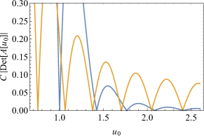
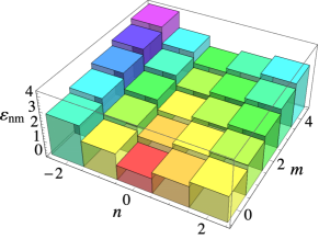
Figure 3: (a) For square well boundary conditions with $L_{2}=-3.1\sqrt{2}$ and $L_{1}=2.1\sqrt{2}$ (in units of $\ell$) we plot $|\mbox{Det}[A_{n}(u_{0})]|$ as function of $u_{0}$ for $n=0$ (blue) and $n=1$ (orange). The zeroes $u_{nm}$ fix the bound-state energies, $\varepsilon_{nm}=u_{nm}\pm\sqrt{n},n=0,1,2,\ldots,m=0,1,2,\ldots$. (b) 3D discrete plot of the bound-state energies $\varepsilon_{nm}$ (negative $n$ means $\varepsilon_{nm}=u_{nm}-\sqrt{n}$). The points $(n,m,\varepsilon_{nm})$ are the center of a unit square placates with half integer vertices, $(n\pm 1/2,m\pm 1/2)$. The square placates are drawn simply to graphically clarify the values of $\varepsilon_{nm}$.

Wavefunctions and Currents.— The spinor wavefunctions and the currents along $y$ corresponding to well height $u_{nm}$ for $(n,m)=(0,0)$ are shown in Fig. 4. The main properties of the wavefunctions are: (1) It is possible to choose the phase such that the upper component of the spinor is real while the lower component is imaginary. This implies that the current along $x$ vanishes, as it should for bound states. (2) Parity symmetry (or antisymmetry) is not exact for the wave functions around $z=0$. The density $\rho(z)=\psi^{\dagger}_{0}(z)\psi_{0}(z)$ is not perfectly symmetric and the current density $J_{y}(z)=\psi^{\dagger}_{0}(z)\sigma_{y}\psi_{0}(z)$ is not perfectly antisymmetric, hence the total (integrated) current $I_{y}$ does not vanish. (With the particular choice of parameters adopted here we get $I_{y}=0.00737326$). The reason for this is that the energy levels are degenerate $\varepsilon(k_{y})=\varepsilon(-k_{y})$ and the corresponding quantities for $\pm k_{y}$ are related:

$$\rho(z;-k_{y})=\rho(-z;k_{y}),\ \ J_{y}(z;-k_{y})=-J_{y}(-z;k_{y}).$$ (21)

Hence, the (incoherent) weighted sums of contributions from $\pm k_{y}$ satisfy the pertinent symmetries, and hence $I_{y}=0$ for the weighted sums. In principle, $\rho(z)$ and $J_{y}(z)$ can be measured together with dipole transition rates (see discussion and illustration in the SM SM ). Therefore, graphene Landau wavefunctions with non-integer orders can be probed.

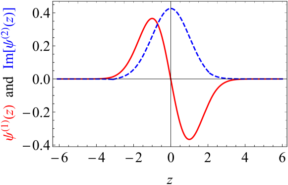
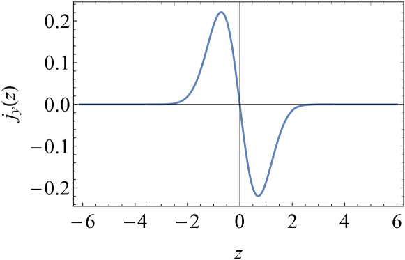
Figure 4: For the potential strength $u_{0}=u_{n=0,m=0}=1.0013$ [the first blue zero in Fig. 3(a)] and width $L_{2}=-3.1\sqrt{2},\ L_{1}=2.5\sqrt{2}$ we plot (a) the upper component (red) and $-i$ times the lower component (blue) of the wavefunction $\psi_{10}(z)$, and (b) the current $J_{y}(z)$ of the state $\psi_{00}(z)$. Since $u_{00}$ is small, the wave functions and current seem to have perfect symmetry around $z=0$ but, strictly speaking, they are not (see see discussion in the text and Ref.SM ).

Summary and Conclusions.— We have developed a formalism for studying electron Klein bound states in single layer graphene subject to a symmetric 1D square-well potential, in the absence as well as in the presence of an external magnetic field. This study completes and adds novel concepts to the analysis of chiral tunneling reported Ref. Katsnelson_06 . In the absence of magnetic field, an analytic expression is derived for the wavefunctions of the ground and excited states, and a beautiful symmetry between the two components of the (pseudo-)spinor is exposed. The consequences of parity non-invariance and time reversal invariance are elucidated, and photon absorption inducing $E1$ transition between two levels is worked out. In the presence of an external uniform perpendicular magnetic field, an analytic expression for the wavefunctions is derived for a discrete (albeit infinite) sequence of potential strengths $u_{0}=\{u_{nm}\}$ $n,m=0,1,2,\ldots$. The Landau functions (in graphene) with non-integer orders and imaginary argument appearing in Eq. (19) are thereby exposed to experimental probes. Exact numerical calculations valid for every potential strength are carried out in the supplemental material SM , and the importance of the symmetry (21) is stressed.

Our results apply directly to the propagation of light waves in periodic waveguide optical structures. Transport of light in a 2D binary photonic superlattice with two interleaved lattices $A$ and $B$ is realized by a sequence of equally spaced waveguides with alternating deep/shallow peak refractive index changes. Propagation of monochromatic light waves is well-described by the scalar wave equation in the paraxial approximation. The tight-binding limit results in coupled-mode equations for the fundamental-mode field amplitudes which are functions of a discrete set of integer variables, and approximating these with a continuous variable rather than as an integer index yields a 2D Dirac equation with an external electrostatic potential Longhi_10 ; Longhi_11 . This yields the same mathematical formalism used to describe graphene.

Acknowledgments: We would like to thank Mikhail I. Katsnelson, Jean Nöel Fuchs Ken Shiozaki and Ady Stern for illuminating discussions. This work was supported in part by a grant from the DFG through the DIP program (FO703/2-1).

References

(1)
M. I. Katsnelson, K. S. Novoselov, and A. K. Geim,
Nature Physics 2, 620 (2006).
(2)
J. M. Pereira Jr., V. Mlinar, F. M. Peeters, P. Vasilopoulos,
Phys. Rev. B 74, 045424 (2006).
(3) M. Ramezani Masir, P Vasilopoulos and F. M. Peeters,
New Journal of Physics, 11, (2009).
(4)
M. Barbier, P. Vasilopoulos and F. M. Peeters,
Phil. Trans. R. Soc. A 368, 5499 (2010).
(5)
H. C. Nguyen, M. T. Hoang, and V. L. Nguyen,
Phys. Rev. B 79, 035411 (2009).
(6)
C. Gutièrrez, L. Brown, C-J Kim, J. Park and A. N. Pasupathy,
Nature Phys. 12, 1069, (2016).
(12)
Riazuddin, “Dirac equation for quasi-particles in graphene in an external electromagnetic field and chiral anomaly”, arXiv:1105.5956.
(13)
Y. B. Band and Y. Avishai, Quantum Mechanics, with Applications
to Nanotechnology and Quantum Information Science,
(Academic Press – Elsevier, 2013), Sec. 7.9.4.
(14) V. Barone and O. Hod et al,
Nano Letters 6, No.12 (2006).
(15)
E. Sadurni,
Revista Mexicana de Fisica 61, 170-181 (2015).
(17) F. W. J. Olver, Uniform Asymptotic Expansions for Weber Parabolic Cylinder Functions of Large Orders, Journal of Research of the National Bureau of Standards B. Mathematics and Mathematical Physics, 63B, No.2, October-December 1959.
(18)
The reason is that there are two inequivalent representations of the 2D Dirac matrices. Parity operation carries valley , and its conservation can be restored if valley degeneracy is incorporated in the Lagrangian, when it is built upon both representations Riazuddin_18 .