Exploring anomalies by many-body correlations

Abstract

The quantum anomaly can be written alternatively into a form violating conservation laws or as non-gauge invariant currents seen explicitly on the example of chiral anomaly. By reinterpreting the many-body averaging, the connection to Pauli-Villars regularization is established which gives the anomalous term a new interpretation as arising from quantum fluctuations by many-body correlations at short distances. This is exemplified by using an effective many-body quantum potential which realizes quantum Slater sums by classical calculations. It is shown that these quantum potentials avoid the quantum anomaly but approaches the same anomalous result by many-body correlations. A measure for the quality of quantum potentials is suggested to describe these quantum fluctuations in the mean energy. Consequently quantum anomalies might be a short-cut way of single-particle field theory to account for many-body effects. This conjecture is also supported since the chiral anomaly can be derived by a completely conserving quantum kinetic theory.

I Introduction

I.1 Anomalies

Anomalies are a puzzling discovery in quantum field theory. Certain classical symmetries and conservation laws are broken if the fields become quantized and have been named anomalies. They have a long history starting with investigations of pion decays Steinberger (1949); Adler (1969); Bell and Jackiw (1969), for an overview see Bertlmann (2000). These anomalies are important for the description of a variety of experiments. Besides the neutral pion decay also the spontaneously broken axial $U(1)$ symmetry in QCD should be mentioned seen in no parity doubling of baryons and no related Goldstone boson ’t Hooft (1976) as well as the Kaon decay Wess and Zumino (1971). The chiral anomaly as breaking of chiral symmetry Adler (1969); Leutwyler (1994) has recently gained a renewed interest in condensed matter physics as excitation of chiral mass-less Fermions in the class of Weyl semi-metals Xu et al. (2015); Lu et al. (2015); Lv et al. (2015); Huang et al. (2015); Weng et al. (2015). It was predicted in Wan et al. (2011) and experimentally interpreted Huang et al. (2015); Xu et al. (2017); Gooth et al. (2017) as having observed chiral anomaly. This has led to an enormous theoretical activity Başar et al. (2014); Johansson et al. (2019); Fröhlich and Pedrini (2000) describing e.g. anomalous transport Alekseev et al. (1998); Kim et al. (2013); Landsteiner (2016a); Gorbar et al. (2018); Morawetz (2016, 2019a), the relation of chiral anomaly and quantized Hall effects Abouelsaood (1985); Moroz et al. (2015) up to chiral heat effect Kimura and Nishioka (2012).

The anomalies lead to anomalous Ward identities Bardeen (1969a); Dolan and Jackiw (1974) and destroy the gauge invariance Wess and Zumino (1971); Preskill (1991) seen also in trace anomalies Bastianelli and van Nieuwenhuizen (1993). One can either formulate the theory consistent or covariant Bardeen and Zumino (1984); Randjbar-Daemi and Strathdee (1997); Adam (1998); Ekstrand (2000); Takeuchi and Endo (2017) dependent whether one accepts alternatively violation of gauge invariance or violation of conservation laws. Furthermore the acceptance of anomalies does not guarantee renormalizability of the theory Gross and Jackiw (1972); Becchi et al. (1981).

Therefore it is highly desirable to formulate the theory free of anomalies or re-describe the experimental facts by a consistent theory. In this respect various anomaly cancellations have been proposed. In electro-weak interaction of the standard model the demand of anomaly-free formulation restricts the fermionic content Bertlmann (2000). Nonlocal counter-terms of gauge fields have been used to compensate anomalies Krasnikov (1985). Extending the initial phase space Moshe and Oz (1989) or using higher dimensions, cancellations Green et al. (1985) have been also worked out. Due to the axial non-conservation sometimes the chiral anomaly is called also mixed axial-gravitational anomaly and claimed to violate Lorentz symmetry Zyuzin and Burkov (2012); Jho et al. (2017); Xu et al. (2017); Gooth et al. (2017). In Del Cima et al. (2017) it has been shown that a proper subtraction scheme of the infrared divergences shows that corresponding extra terms do not appear. In fact the Lorentz-invariant chiral kinetic theory can be derived from the quantum kinetic approach Gao et al. (2012); Chen et al. (2013); Manuel and Torres-Rincon (2014); Gao et al. (2017); Hidaka et al. (2017); Huang et al. (2018); Morawetz (2019a) leading to the chiral anomaly by many-body correlations. A hint that the anomalies can be possibly explained by many-body effects is also the observation that they can be described by the Dirac sea Nielsen and Ninomiya (1983); Vladimirov (1990); Adam et al. (1993).

We conclude that besides the well worked out mathematical appearances of anomalies as triangle graphs in field theoryBardeen (1969a); Adler (1969); Bardeen and Zumino (1984); Bastianelli and van Nieuwenhuizen (1993); Bertlmann (2000); Fujikawa and Suzuki (2004), the physical origin of anomalies is still a matter of debate. Therefore it is the motivation of this paper to draw the attention to a possible different scenario. Given the experimental facts, we believe that the anomalies describe real physics. However, it is the question whether it has to appear as anomalous or whether the same physics can be described by ordinary means. Let us employ an analogy. Pairing in superconductors is conveniently described by anomalous propagators to achieve the Gorkov equations or correspondingly the Beliaev equations for Bose condensates. These propagators violate the number conservation and are inconsistent in the above sense. Nevertheless they lead to correct equations. Recently it has been shown that one can arrive at the same equations by a completely conserving theory of multiple corrected T-matrix Lipavský (2008); Morawetz (2011); Šopík et al. (2011) with equivalent results Morawetz (2010); Männel et al. (2013). This illustrates that the anomalous propagators are a theoretical short-cut to the right result though adopting inconsistent steps.

Analogously we will propose here that the quantum anomaly might be a short cut way to describe correct physics. We will propose to consider it as a many-body correlation phenomenon. Let us illustrate this in terms of the well-discussed chiral anomaly before we restrict to the non-relativistic case in the paper.

I.2 Field theoretical approach

Relativistic Fermions with zero mass and consequently linear dispersion have a definite chirality by parallel or anti-parallel spin and motion directions Weyl (1929). The left and right-handed projections are realized by $(1\mp\gamma_{5})/2$ with $\gamma_{5}=i\gamma^{0}\gamma^{1}\gamma^{2}\gamma^{3}$. The chiral or axial transformation

$$\Psi^{\prime}(x)={\rm e}^{i\alpha(x)\gamma_{5}}\Psi(x)$$ (1)

leads to the axial current $J_{5}=\overline{\Psi}\gamma^{\mu}\gamma^{5}\Psi$ which changes the classical action $S^{\prime}=S+\int\alpha(x)\nabla_{\mu}J_{5}^{\mu}$. This results into the conservation law

$$\nabla_{\mu}J_{5}^{\mu}=2im\overline{\Psi}\gamma^{5}\Psi\to 0,\quad{\rm for}\quad m\to 0$$ (2)

for mass-less Dirac particles. The quantum averaging in contrast,

$$\langle\partial_{\mu}J_{5}^{\mu}\rangle = 2im\langle\overline{\Psi}\gamma^{5}\Psi\rangle\to{e^{2}\over 16\pi^{2}\hbar^{2}c}\varepsilon^{\mu\nu\alpha\beta}F_{\mu\nu}F_{\alpha\beta}$$ (3)

$$= {e^{2}\over 2\pi^{2}\hbar^{2}}{{\bf E}\cdot{\bf B}}\quad{\rm for}\quad m\to 0,$$

shows a non-vanishing anomalous term obviously due to quantum fluctuations in the average.

The origin is best seen from Pauli-Villars regularization where we subtract from the Dirac Lagrangian for $\Psi$ a massive (${M\to\infty}$) field $\Phi$ Kafiev (1991); Bertlmann (2000); Fujikawa and Suzuki (2004)

$${\cal L}=i{\bar{\Psi}}({\not{\partial}}-ie{\not{A}})\Psi-i{\bar{\Phi}}({\not{\partial}}-ie{\not{A}})\Phi+{M}{\bar{\Phi}}\Phi.$$ (4)

For the chiral current we calculate ${\rm Tr}\gamma^{5}G_{12}$ with $(i{\not{\partial}}_{1}-{M}+e{\not{A}}_{1})G_{12}=-\delta_{12}$ iteratively by $G=G_{0}+G_{0}e{\not{A}}G$ and $G_{0}=-({\not{p}}-{M})^{-1}$. Due to the trace the first non-vanishing terms are of fourth-order

$$\langle\partial_{\mu}J_{5}^{\mu}\rangle=8\epsilon^{\kappa\lambda\mu\nu}\int{d^{4}qd^{4}r\over(2\pi)^{4}}{\rm e}^{irx}er^{\nu}A_{q-r}^{\mu}q^{\lambda}eA_{-q}^{\kappa}$$

$$\times\int{d^{4}p\over(2\pi)^{4}}{{M}^{2}\over(p^{2}-{M}^{2})((p+q)^{2}-{M}^{2})((r+p)^{2}-{M}^{2})}$$

$$=-{1\over 4\pi^{2}\hbar^{2}}\epsilon^{\kappa\lambda\mu\nu}\partial_{x}^{\nu}eA^{\mu}\partial_{x}^{\lambda}eA^{\kappa}$$

$$=-{e^{2}\over 16\pi^{2}\hbar^{2}}\epsilon^{\kappa\lambda\mu\nu}F^{\nu\mu}F^{\lambda\kappa}={e^{2}\over 2\pi^{2}\hbar^{2}}{{\bf E}\cdot{\bf B}}$$ (5)

where one calculates the integral in the $M\to\infty$ limit with $\int d^{4}p/(p^{2}+M^{2})^{3}=\pi^{2}/2M^{2}$. This means it comes from divergences up to fourth adiabatic order (renormalization) which can be expressed by anomalous triangle graphs Jensen (2012); Başar et al. (2014); Landsteiner (2016b) known as Adler-Jackiw-Bell anomaly Adler (1969); Bell and Jackiw (1969); Nielsen and Ninomiya (1983). The origin is clearly the behaviour at small distances or large momenta. This chiral anomaly can be based on anomalous Ward identities which quantum vector or axial vector fields obey. Only exclusively one of them can be made normal Bardeen (1969b). In fact, the rate of chirality (5) can be rewritten explicitly Morawetz (2019b)

$$\partial_{t}n_{5}+{{\bf\nabla}}\cdot({\bf j}+{\bf j}_{\rm anom})=0.$$ (6)

Using the vector and scalar potentials ${\bf B}=\nabla\times{\bf A},{\bf E}=-\dot{{\bf A}}-\nabla\phi$, the anomalous current

$${\bf j}_{\rm anom}={e^{2}\over 2\pi^{2}\hbar^{2}}\left(\frac{1}{2}\dot{{\bf A}}\times{\bf A}-\phi{{\bf\nabla}}\times{\bf A}\right)$$ (7)

is non gauge-invariant. So one can choose either to accept a non-conserving rate equation (5) or alternatively a conserving rate equation (6) but with a non gauge-invariant current (7).

I.3 Many-body approach

The same anomalous result (3) can be obtained by many-body effects without anomalous behaviour. Heuristically it can be seen easily Fukushima et al. (2008) considering a parallel electric and magnetic field which changes the chirality. The Fermi momentum of the right-handed Fermions increases in the electric field $p_{\rm F}=eEt$ with opposite direction for left-handed ones. The density of left and right-handed Fermions is the product of the longitudinal phase-space density, $dN_{R}/dz=p_{\rm F}/2\pi\hbar$, and the density of Landau levels in traverse direction, $d^{2}N_{R}/dxdy=eB/2\pi\hbar$, such that the rate of chirality $N_{5}=N_{R}-N_{L}$ is

$${dn_{5}\over dt}={d^{4}N_{5}\over dtd^{3}x}=2{\dot{p}_{\rm F}\over 2\pi\hbar}{eB\over 2\pi\hbar}={e^{2}\over 2\pi^{2}\hbar^{2}}{\bf E}\cdot{\bf B}$$ (8)

which agrees with (3). We see that a completely conventional reasoning leads to the same result as obtained by anomaly. The quantum kinetic derivation of this result without any non-conserving assumptions can be found in Morawetz (2019a).

The ${\bf E}{\bf B}$ term is also the basis of the experimental interpretation Huang et al. (2015); Xu et al. (2017); Gooth et al. (2017) of having observed chiral anomaly and breaking of conservation laws like mixed axial-gravitational anomaly. The electrodynamics assuming explicitly a chiral breaking term has been treated in Qiu et al. (2017). The well investigated path from symmetry-violating assumptions to final ‘non-conservation‘ form Zyuzin et al. (2012) was in a sense misleading if one sees it as an unique signal of violation of conservation laws. One cannot conclude backwards from the observed term (3) to a symmetry-breaking field-theoretical assumption since (5) appears also by a conserving theory without the described field-theoretical assumptions Morawetz (2019a).

I.4 Conjecture and outline

If the physical origin of the anomalous term is the behaviour at small distances and the quantum fluctuations by many-body correlations, one should be able to get the anomalous results by ordinary many-body treatments. We want here to investigate more in detail how the quantum averaging over the wave function can consistently be performed within a many-body treatment. In fact we will show that a proper treatment of such many-body averaging renormalizes the divergence at small distances and no anomaly appears. The term (6), however, shows up nevertheless since it has a many-body origin. Therefore the conjecture is proposed that the anomalies are short-cut ways of single-particle field theory to a many-body effect. In the single-particle treatment they appear as anomalous, in many-body treatment they appear naturally without anomaly.

The outline of the paper is as follows. In the next chapter II the nonrelativistic anomalies are re-derived by many-body correlations and the statistical sum. Conditions are discussed dependent on dimensionality, power law of potentials and perturbation order. This results into an anomalous energy shift of $\frac{1}{8}E_{0}$. In chapter III we show that the use of quantum potentials avoid this anomaly but leads naturally to this energy shift due to the finite value of the potential at small distances. This finite value is caused by quantum fluctuations which are represented by quantum potentials discussed in binary and ternary order. Chapter IV summarizes the results. Appendix A provides integrals occurring in the treatment of chapter II. Appendix B discusses the derivation of quantum potentials on binary and ternary level separately for Maxwellian and for Fermi correlations.

II Anomaly by statistical sum

First we observe that the averaging over a many-body statistical operator with kinetic $\hat{E}$ and potential $\hat{V}$ energy can be written as inverse La-Place transform

$$z={\rm Tr}\,{\rm e}^{-\beta(\hat{E}+\hat{V}-\mu\hat{N})}={\rm Tr}\!\!\!\!\!\int\limits_{-i\infty+\epsilon}^{i\infty+\epsilon}\!\!{dM\over 2\pi i}{\rm e}^{\beta(M\!+\!\mu\hat{N})}{1\over\hat{E}+\hat{V}+M}$$

$$=\!{\rm Tr}\!\!\!\!\!\int\limits_{-i\infty+\epsilon}^{i\infty+\epsilon}\!\!\!{dM\over 2\pi i}{\rm e}^{\beta(M\!+\!\mu\hat{N})}\!\left({1\over\hat{E}\!+\!M}-{1\over\hat{E}\!+\!M}V{1\over\hat{E}\!+\!M}\pm....\right)$$ (9)

where we expand with respect to the interaction and assume that it commutes with the number operator. The vanishing statistical averaging corresponds to the high-temperature limit $\beta\to 0$ or alternatively to $M\to\infty$. The latter one takes the role of the large mass of Pauli-Villars regularization. To see this, consider the pure quantum state expectation Kirzhnitz and Shpatakovskaya (1996) in $D$-dimensions

$${\rm Tr^{\rm QM}\hat{A}}\!=\!\!\int\!\!\!{d^{D}p\over(\!2\pi\hbar\!)^{D}}\langle p|\hat{A}|p\rangle=\!\!\int\!\!\!{d^{D}\!xd^{D}\!p\over(2\pi\hbar)^{D}}{\rm e}^{-{i\over\hbar}{\bf p}{\bf x}}\langle x|\hat{A}|x^{\prime}\rangle{\rm e}^{{i\over\hbar}{\bf p}{\bf x}^{\prime}}.$$ (10)

If the observable $\hat{A}$ does not contain any explicit $\hbar$, one expects $(2\pi\hbar)^{D}{\rm Tr\hat{A}}-\lim\limits_{\hbar\to 0}(2\pi\hbar)^{D}{\rm Tr\hat{A}}=0$. A violation of this zero represents the quantum anomaly.

To investigate it further, we combine the many-body mixed state (9) and the quantum-mechanical pure state (10) averaging

$$W^{(1)} =(2\pi\hbar)^{D}z-\lim\limits_{\hbar\to 0}(2\pi\hbar)^{D}z$$

$$=\sum\limits_{n=0}^{\infty}(-1)^{n}\int{dM\over 2\pi i}{\rm e}^{\beta M}W_{n}$$ (11)

with

$$W_{n} =\sum\limits_{n_{1}}n_{1}^{n}{\rm e}^{\beta\mu n_{1}}\!\int\!\!d^{D}pd^{D}x$$

$$\times\left[{1\over n_{1}{({\bf p}\!-\!i\hbar\partial_{{\bf x}})^{2}\over 2m}\!+\!M}V(x){1\over n_{1}{({\bf p}\!-\!i\hbar\partial_{{\bf x}})^{2}\over 2m}\!+\!M}V...\right.$$

$$-\,\left.{1\over n_{1}{(p)^{2}\over 2m}+M}V(x){1\over n_{1}{(p)^{2}\over 2m}+M}V\right]$$ (12)

where we have used the non-relativistic kinetic energy $\hat{E}=\hat{p}^{2}/2m$ as example. The relativistic dispersion works analogously. We have commuted the $\exp{(-i{\bf p}{\bf x}/\hbar)}$ factor in (10) through the kinetic energy factors. The sum runs over the number of Fermions $n_{1}=0,1$ or Bosons $n_{1}=0,1,2...$.

Now we assume a momentum dependence of the Fourier transformed potential in the form of a power law

$$V(q)=E_{0}a_{0}^{D}c_{d}q^{-{\alpha}}$$ (13)

with a typical energy $E_{0}$ and length scale $a_{0}$. This would be the Bohr radius $a_{0}=a_{B}$ and $E_{0}=Ryd=e^{2}/4\pi\epsilon_{0}a_{B}$ for Coulomb potentials in D=1,2,3 dimensions with the numerical factor $c_{d}=2^{D-1}\pi$. The Fourier transformation (12) in dimensionless momentum ${\bf k}\to{\bf k}\sqrt{n_{1}/2mM}$ reads then

$$W_{n}={(2\pi\hbar)^{D}c_{d}^{n}\over 2^{\frac{n}{2}(\alpha-D)}}E_{0}^{s+1}\sum\limits_{n_{1}}{{\rm e}^{\beta\mu n_{1}}\over n_{1}^{s+1}}M^{s}\,I_{n}^{(D)}(\alpha)$$ (14)

with

$$s=\frac{n}{2}(D-\alpha-2)-1$$ (15)

and

$$I_{n}^{(D)}(\alpha)=\!\!\int\!\!\!{d^{D}k_{1}\over(2\pi)^{D}k_{1}^{\alpha}}...{d^{D}k_{n}\over(2\pi)^{D}k_{n}^{\alpha}}{d^{D}p\over 1\!+\!p^{2}}\delta\left(\Sigma_{i=1}^{n}{\bf k}_{i}\right)$$

$$\times\!\!\left[{1\over 1\!+\!({\bf p}\!+\!{\bf k}_{1})^{2}}...{1\over 1\!+\!({\bf p}\!+\!{\bf k}_{1}\!+\!...\!+\!{\bf k}_{n})^{2}}\!-\!{1\over(1\!+\!p^{2})^{n}}\right].$$ (16)

One can understand this integral as a ring-graph of $n$ propagators interacting $n$ times with external potentials as illustrated in figure 1, first considered in Bardeen (1969a).

Figure 1: Propagators interacting with external potentials in a ring according to (16).

The expression $W^{(1)}$ describes the anomaly in the normalization of the statistical operator or the completeness. The corresponding term for the mean energy is conveniently expressed as $W^{(H)}=-\partial_{\beta}W^{(1)}$. If we are interested in the anomaly of the momentum, we have an additional momentum factor which requires $s\to s+1/2$ and a fore-factor $\sqrt{2}\hbar/a_{B}$ as well as modified integrals (16) by an additional $p$ factor.

Performing the inverse La Place transform (11) we obtain finally

$$W^{(1)}=\sum\limits_{n_{1},n=1}^{\infty}{(-c_{d})^{n}(2\pi\hbar)^{D}\over 2^{\frac{n}{2}(\alpha-D)}}{{\rm e}^{\beta\mu n_{1}}I_{n}^{(D)}(\alpha)\over\Gamma(-s)(E_{0}\beta n_{1})^{1+s}}.$$ (17)

Let us now discuss the $M\to\infty$ or ${\beta}\to 0$ analogous to the Pauli-Villars regularization. This will produce a non-vanishing anomaly only for certain combinations of dimensions $D$, power of the momentum in the potential $\alpha$ and the order of terms $n$ in the sum (17).

One sees the dependence on $\beta$ as

$$W^{(1)}=(2\pi\hbar)^{D}\delta z \sim \beta^{-1-s}$$

$$W^{(H)}=(2\pi\hbar)^{D}\delta H \sim (1+s)\beta^{-2-s}$$

$$W^{(p)}=(2\pi\hbar)^{D}\delta p \sim \beta^{-\frac{3}{2}-s}$$ (18)

which means that one gets a nonzero anomaly for the normalization $\delta z$, the energy $\delta E$ and the momentum $\delta p$ only for the combinations

$$\delta z \neq 0:\forall n,D=2+\alpha$$

$$\delta H \neq 0:n=1,D=\alpha\,\,{\rm or}\,\,n=2,D=\alpha+1$$

$$\delta p \neq 0:n=1,D=2+\alpha.$$ (19)

For any sensible potential the relation for the anomaly in the normalization $\delta z$ is not fulfilled. Also the case of momentum anomaly is zero due to the vanishing integral (82). We get therefore the anomaly only for the mean value of the energy

$$\langle H\rangle ={\operatorname{Tr}{\hat{H}\hat{\rho}}\over z}\!+\!\Delta H,\,\,{\rm for}\,\,n=1,D=\alpha\,{\rm or}\,n=2,D=\alpha\!+\!1.$$ (20)

Let us discuss this anomaly in each dimension. In three dimensions ${D}=3$ and Coulomb ${\alpha}=2$ interaction, the integral (16) is given by (74) and one obtains

$$\Delta H={W^{(H)}\over(2\pi\hbar)^{3}}=\frac{1}{8}E_{0}$$ (21)

a result reported in Kirzhnitz and Shpatakovskaya (1996) with a factor of $2$ due to spin which we omit here. Summarizing, the mean energy $H$ shows a quantum anomaly but not the normalization $z$.

In two dimensions with a potential of ${\alpha}=1$ one finds analogously

$$W_{n}^{(1)}\sim{\beta}^{n/2}\to 0\,{\rm and}\,W^{(H)}_{n}\sim{\beta}^{n/2-1}\neq 0\,{\rm for}\,n=2$$ (22)

and for ${\alpha}=2$

$$W_{n}^{(1)}\sim{\beta}^{n}\to 0\,{\rm and}\,W^{(H)}\sim{\beta}^{n-1}\neq 0\,{\rm for}\,n=1.$$ (23)

In one dimensions we do not have any anomaly for any potential. Indeed, considering $\alpha=1$ we have

$$W_{n}\sim{\beta}^{n}\to 0,{\rm and}\,W^{(H)}\sim{\beta}^{n-1}\neq 0,{\rm for}\,n=1$$ (24)

but $I_{1}^{(1)}(1)=0$ due to (81). For $\alpha=2$ all anomalies vanish in 1D due to $W_{n}\sim{\beta}^{\frac{3}{2}n}\to 0$ and $W^{(H)}_{n}\sim{\beta}^{\frac{3}{2}n-1}\to 0$. The Fourier transform of the Coulomb potential in 1D is $\alpha=0$ but $V(q)\sim{\rm sign}(q)$ which leads to $I_{2}^{(1)}(0)=0$ as well.

We can conclude that in all discussed cases the anomalies appear due to the large momentum (short distance) divergence of the potential. The results depend on dimensions and the anomaly appears in 2D and 3D but not in 1D and can be understood as a certain limit of the statistical sum. In the following we restrict to the discussion of three dimensions.

III Effective quantum potential

We can now state that a finite behaviour of the potential at small distances realized by quantum potentials cures such anomalies since we will see that they lead to $\alpha=4$ which avoids all cases of anomalies (19). These effective quantum potentials appear if we represent the many-body binary quantum correlations by a classical calculation with an effective quantum potential. Formally there are two ways to achieve this goal. The first way constructs the quantum potential such that the two-particle quantum Slater sum is correctly represented by the classical one with the help of the quantum potential. This results into the Kelbg potential for Maxwellian Coulomb systems Kelbg (1964a, b); Ebeling et al. (1967); Kremp and Kraeft (1968)

$$V_{2}(r) = {E_{0}a_{0}\over r}\left[1-{\rm e}^{-\left({r\over l}\right)^{2}}+\sqrt{\pi}\,{r\over l}\,{\rm erfc}\left({r\over l}\right)\right]$$ (27)

$$= E_{0}a_{0}\left\{\begin{array}[]{c}{1\over r}+o(r^{-3})\cr{\sqrt{\pi}\over l}-{r\over l^{2}}+o(r^{2})\end{array}\right.$$

where the coordinate is scaled by the thermal wave length $l^{2}=2\hbar^{2}/mT$. Improvements and systematic applications can be found in Kraeft et al. (1986); Kraeft and Kremp (1968); Ortner et al. (2000).

The second way is to use a statistical equivalence of quantum $N$-particle systems with an $N+1$-particle classical system Morawetz (2002). There it was found that the quantum potentials are just successive convolutions of the (Coulomb) potential $V^{c}(x)$ with the binary distribution $\rho^{(2)}(x)$. If we use the non-degenerate Maxwell correlation

$$\rho^{(2)}(r)\! = \!\!\int\!\!\!{dp\over(2\pi\hbar)^{3}}{\rm e}^{ipr/\hbar}{\rm e}^{-\beta{p^{2}\over 2mT}}={1\over\pi^{3/2}l^{3}}{\rm e}^{-r^{2}/l^{2}}$$ (28)

the Kelbg potential (27) appears as

$$V_{2ab}(r) \propto \sum\limits_{c}\int{dx_{1}}\rho^{(2)}_{bc}(x_{1})V^{c}_{cb}(x_{1})V^{c}_{ca}(x_{1}+r)$$ (29)

with the quantum number, e.q. being charges, indicated by latin subscripts. As calculated in appendix B, using the Fermi function at $T=0$, we obtain instead of (28) the potential

$$V_{2\rm f}(r)\! = \!{E_{0}a_{0}\over 2r}\!\left[\!2\!+\!{\pi r\over 2l_{\rm F}}\!-\!{\cos{r\over l_{\rm F}}}\!-\!{l_{\rm F}\over r}\sin{r\over l_{\rm F}}\!-\!{r\over l_{\rm F}}Si\left(\!{r\over l_{\rm F}}\!\right)\!\right]$$ (32)

$$= E_{0}a_{0}\left\{\begin{array}[]{c}{1\over r}+o(r^{-3})\cr{\pi\over 4l_{\rm F}}-{r\over 6l_{\rm F}^{2}}+o(r^{2})\end{array}\right.$$

where the coordinate scales with the inverse Fermi momentum $l_{\rm F}=\hbar/p_{\rm F}$ and the sinus integral is $Si(x)=\int_{0}^{x}dt\sin{t}/t$.

This scheme allows to construct besides the binary quantum potential also the next (ternary) order

$$V_{3ab}(r)\propto\sum\limits_{cd}\int{dx_{1}dx_{2}}\rho_{dc}(x_{1})V^{c}_{cd}(x_{1})V^{c}_{cb}(x_{1}+x_{2})$$

$$\times\rho_{bd}(x_{2})V^{c}_{ca}(x_{1}+x_{2}+r)$$ (33)

which leads with (28) to

$$V_{3}(r) ={E_{0}a_{0}\over r}\left[{\rm erf}^{2}\!\left(\!{x\over\sqrt{2}}\!\right)\!+\!{2^{3/2}x\over\sqrt{\pi}}\!\int\limits_{x}^{\infty}\!{dz\over z}{\rm e}^{-{z^{2}\over 2}}{\rm erf}\!\left({z\over\sqrt{2}}\!\right)\right]$$

$$=E_{0}a_{0}\left\{\begin{array}[]{c}{1\over r}+o(r^{0})\cr{\sqrt{8}\,{\rm ln}(1+\sqrt{2})\over\sqrt{\pi}l}-{2r\over\pi l^{2}}+o(r^{2})\end{array}\right.$$ (36)

calculated in appendix B. The corresponding ternary order for Fermi correlations reads

$$V_{3\rm f}(r) ={E_{0}a_{0}\over r}{4\over\pi^{2}+4}\int\limits_{0}^{1}{dx\over x}\left[x+\left(1-x^{2}\right){\rm artanh}x\right]$$

$$\times\left[2+\pi{xr/l_{\rm F}}-2\cos{({xr/l_{\rm F}})}-2x{r\over l_{\rm F}}{\rm Si}\left({xr/l_{\rm F}}\right)\right]$$

$$=E_{0}a_{0}\left\{\begin{array}[]{c}{1\over r}+o(r^{0})\cr{4\pi\,(1+2{\rm ln}2)\over 3(4+\pi^{2})l_{\rm F}}-{2r\over(4+\pi^{2})l_{\rm F}^{2}}+o(r^{2})\end{array}\right..$$ (39)

The results (32) and (39) are not yet reported while the ones (27) and (36) had been presented in Morawetz (2002). The quantum potential of binary and ternary correlations are compared in figure 2 where the finite limits at small distances are shown. The ternary order somewhat improves the binary quantum potential and leads to somewhat less binding behaviour.

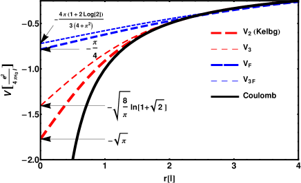
Figure 2: The comparison of the Kelbg potential (27) of binary correlations together with the next (ternary) order correlation potential (36), the Fermi potential (32) and the Coulomb potential. For the Kelbg and ternary potential the scale is $l=\hbar\sqrt{2\beta/m}$ and for the Fermi potential $l=l_{\rm F}=\hbar/p_{\rm F}$. The finite value at zero distance is explicitly indicated.

This means that the Coulomb divergence at small distances is cured due to quantum fluctuations brought by many-body correlations. Please note that this is the opposite limit than the large-distance Coulomb behaviour which is cured by screening. This finite behaviour at small distance translates into a higher potential decay at large momenta. In fact, the Fourier transform of the binary potentials read

$$V_{2}(q) ={8\pi E_{0}a_{0}\hbar^{3}\over q^{3}l}D\!\left(\!{ql\over 2\hbar}\!\right)={E_{0}a_{0}}\!\left\{\!\begin{array}[]{c}{8\pi\hbar^{4}\over l^{2}q^{4}}\!+\!o(q^{-6})\cr{4\pi\hbar^{2}\over q^{2}}\!-\!{2\pi l^{2}\over 3}\!+\!o(q^{2})\end{array}\right.$$ (42)

and

$$V_{3}(q) ={32E_{0}a_{0}\hbar^{3}\over\sqrt{\pi}q^{3}l}\int\limits_{0}^{\infty}du{\rm e}^{-u^{2}}D(u)\,{\rm ln}\left|{(u+{ql\over 2})\over(u-{ql\over 2})}\right|$$

$$={E_{0}a_{0}}\left\{\begin{array}[]{c}{16\hbar^{4}\over l^{2}q^{4}}+o(q^{-6})\cr{4\pi\hbar^{2}\over q^{2}}-{2(2+\pi)\over 3}l^{2}+o(q^{2})\end{array}\right.$$ (45)

with the Dawson function $D(x)={\rm e}^{-x^{2}}\int\limits_{0}^{x}dy{\rm e}^{y^{2}}$. Analogously one obtains for the Fermi potential

$$V_{2\rm f}(q) ={2\pi E_{0}a_{0}\hbar^{2}\over q^{2}}\left(1+{p_{\rm F}^{2}-q^{2}\over 2qp_{\rm F}}{\rm ln}\left|{p_{\rm F}+q\over pf-q}\right|\right)$$

$$={E_{0}a_{0}}\left\{\begin{array}[]{c}{4\pi\hbar^{4}\over 3l_{\rm F}^{2}q^{4}}+o(q^{-5})\cr{4\pi\hbar^{2}\over q^{2}}-{4\pi l_{\rm F}^{2}\over 3}+o(q^{2})\end{array}\right.$$ (48)

and

$$V_{3\rm f}(q) ={16\pi E_{0}a_{0}\hbar^{3}\over(4\!+\!\pi^{2})q^{3}l}\!\!\int\limits_{0}^{1}\!\!\!dx\!\left[x\!+\!\left(1\!-\!x^{2}\right){\rm artanh}x\right]{\rm ln}{|xp_{\rm F}\!+\!q|\over|xp_{\rm F}\!-\!q|}$$

$$={E_{0}a_{0}}\left\{\begin{array}[]{c}{16\pi\hbar^{4}\over(4+\pi^{2})l_{\rm F}^{2}q^{4}}+o(q^{-6})\cr{4\pi\hbar^{2}\over q^{2}}-{4\pi(12+\pi^{2})\over 3(4+\pi^{2})}l_{\rm F}^{2}+o(q^{2})\end{array}\right..$$ (51)

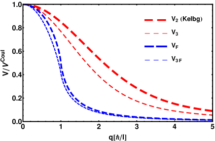
Figure 3: The ratio of the quantum potentials to the Coulomb one in momentum space. For the Kelbg and ternary potential the scale is $l=\hbar\sqrt{2\beta/m}$ and for the Fermi potential $l=l_{\rm F}=\hbar/p_{\rm F}$.

These quantum potentials in momentum space are compared in figure 3. The potentials with Fermi correlations show a faster decay around the Fermi momentum $q=p_{\rm F}$ compared to the Maxwellian ones. We see that all the quantum potentials show a $V(q)\sim 1/q^{4}$ behaviour for large $q$ and a Coulomb behaviour at small $q$. Therefore these quantum potentials lead to $\alpha=4$ and according to the above discussions for the appearance of anomalies they vanish in all cases. Does this mean that the energy shift of the anomaly (21) does not exist? We will see how that will reappear quite ordinarily as the difference of the total energy calculated by quantum potentials compared with the one by the Coulomb potential.

We consider the Hartree correlational energy corresponding to the lowest-order binary quantum potential for homogeneous systems

$$E_{\rm corr}=\frac{1}{2}\int d^{3}r^{\prime}n(r-r^{\prime})V(r^{\prime})=\frac{n}{2}V(q=0)$$ (52)

which is the convolution of the potential with the particle density $n$. According to (42)-(51), the difference of one-particle energies between the quantum potentials and the Coulomb one is

$$E_{1}-E^{c}_{1} = \frac{n}{2}[V_{\rm quant}(q=0)-V^{c}(q=0)]$$ (57)

$$= -E_{0}\left\{\begin{array}[]{rlcc}{1\over 3\sqrt{\pi}}&{a_{0}\over l}&{\rm for}&V_{2}\cr{2+\pi\over 3\pi^{3/2}}&{a_{0}\over l}&{\rm for}&V_{3}\cr{2\over 9\pi}&{a_{0}\over l_{\rm F}}&{\rm for}&V_{2\rm f}\cr{2(12+\pi^{2})\over 9\pi(4+\pi^{2})}&{a_{0}\over l_{\rm F}}&{\rm for}&V_{3\rm f}\end{array}\right.$$

where we have used the densities $n=1/\pi^{3/2}l^{3}$ for $V_{2,3}$ and $n=1/3\pi^{2}l_{\rm F}^{3}$ for $V_{2,3f}$. The kinetic energies subtract identically.

On the other hand we have the potential energy of a single particle $V(r=0)$ as indicated in figure 2. Adding the kinetic energies $3T/2=3E_{0}a_{0}^{2}/l^{2}$ for $V_{2,3}$ and $3p_{\rm F}^{2}/10m=3E_{0}a_{0}^{2}/10l_{\rm F}^{2}$ for $V_{2\rm f}$, we obtain the single-particle energy from (32)-(39)

$$E_{1}=E_{0}\left\{\begin{array}[]{cc}\sqrt{\pi}{a_{0}\over l}+3{a_{0}^{2}\over l^{2}}&{\rm for}\,V_{2}\cr\sqrt{8\over\pi}\,{\rm ln}(1+\sqrt{2}){a_{0}\over l}+3{a_{0}^{2}\over l^{2}}&{\rm for}\,V_{3}\cr{\pi\over 4}{a_{0}\over l_{\rm F}}+{3\over 10}{a_{0}^{2}\over l_{\rm F}^{2}}&{\rm for}\,V_{2\rm f}\cr{4\pi(1+2{\rm ln}2)\over 3(4+\pi^{2})}{a_{0}\over l_{\rm F}}+{3\over 10}{a_{0}^{2}\over l_{\rm F}^{2}}&{\rm for}\,V_{3\rm f}\end{array}\right.$$ (62)

Dividing now (57) by (62) and using the limit of $l\to 0$ corresponding to $\beta\to 0$ of chapter II, which is also the maximum ratio, we get

$${\langle E_{1}-E^{c}_{1}\rangle\over\langle E_{1}\rangle}=-{1\over c}$$ (63)

and therefore

$$\Delta H={\langle E^{c}_{1}\rangle-\langle E_{1}\rangle}={\langle E^{c}_{1}\rangle\over 1+c}$$ (64)

with

$$c=\left\{\begin{array}[]{rccl}{3\pi}&\approx&9.24&{\rm for}\,V_{2}\cr{6\pi\sqrt{2}\,{\rm ln}(1+\sqrt{2})\over(2+\pi)}&\approx&4.57&{\rm for}\,V_{3}\cr{9\pi^{2}\over 8}&\approx&11.10&{\rm for}\,V_{2\rm f}\cr{6\pi^{2}(1+2{\rm ln}2)\over 12+\pi^{2}}&\approx&6.46&{\rm for}\,V_{3\rm f}\end{array}\right..$$ (69)

Comparing with the exact “anomalous” result (21) we would expect $c=7$. The increasing quality of potentials from binary to ternary level is visible. The Maxwellian is less accurate than the Fermi correlation since we had considered Fermi ones in chapter II. We can now suggest to use this ration $c$ of the energy to the deviation of the energy with quantum potentials from the classical Coulomb one as a measure for the quality of the potential to represent quantum fluctuations.

IV Summary

The nonrelativistic quantum anomaly is investigated for combinations of momentum behaviour of potentials, dimensionality, and the order of perturbation. It is found that only for the energy an anomalous shift appears in three dimensions while in one dimension no anomaly is seen. In two dimensions the discussion can be performed analogously. It is seen that the quantum anomaly appears as the large momentum or short distance behaviour of the potential. Quantum potentials are proposed which describe quantum features on a classical level. These quantum potentials lead to a finite value at small distances and cure the Coulomb divergence. The consequence is that no quantum anomaly appears. In contrast, the deviation of the energy with quantum potentials from the energy with the Coulomb potential reflects this anomalous energy shift. In this way the quantum anomalous behaviour is reformulated by normal quantum many-body correlations. It may be a hint that anomalies as such are a theoretical short cut to the right physics but can be formulated equivalently by a more refined many-body treatment. This of course needs further investigation on a more abstract level than considered here. The discussed quantum potentials might be usefull to describe the simulation of strongly correlated quantum systems by classical terms.

Appendix A Integrals

The occurring integrals in chapter II have the form

$$I_{n}^{(D)}(\alpha)=\sum\limits_{p,k_{1},...k_{n}}{\delta(k_{1}+...+k_{n})\over k_{1}^{\alpha}...k_{n}^{\alpha}}{1\over 1+p^{2}}$$

$$\times\left({1\over 1\!+\!({\bf p}\!+\!{\bf k}_{1})^{2}}...{1\over 1\!+\!({\bf p}\!+\!{\bf k}_{1}\!+...\!+\!{\bf k}_{n})^{2}}\!-\!{1\over(1\!+\!p^{2})^{n}}\right)$$ (70)

with $\sum_{p}=\int d^{D}p/(2\pi)^{D}$ Introducing new variables ${\bf p}_{1}={\bf k}_{1}+{\bf p}$, ${\bf p}_{2}={\bf k}_{2}+{\bf p}_{1}$ etc. leads to

$$I_{n}^{(D)}(\alpha)=\sum\limits_{p,p_{1}...p_{n-1}}\left[{1\over 1+p_{1}^{2}}...{1\over 1+p_{n-1}^{2}}-{1\over(1+p^{2})^{n-1}}\right]$$

$${1\over({\bf p}_{1}\!-\!{\bf p})^{\alpha}}{1\over({\bf p}_{2}\!-\!{\bf p}_{1})^{\alpha}}...{1\over({\bf p}_{n\!-\!1}\!-\!{\bf p}_{n\!-\!2})^{\alpha}}{1\over({\bf p}\!-\!{\bf p}_{n\!-\!1})^{\alpha}}{1\over(1\!+\!p^{2})^{2}}$$ (71)

We are going to calculate the integrals for Coulomb potentials $\alpha=2$.

A.1 3D

Lets consider the integrals with increasing $n$ starting with the lowest non-vanishing one

$$I_{2}^{(3)}(2)=\sum_{p,p_{1}}{1\over({\bf p}_{1}\!-\!{\bf p})^{4}}{1\over(1\!+\!p^{2})^{2}}\left[{1\over 1\!+\!p_{1}^{2}}\!-\!{1\over 1\!+\!p^{2}}\right]$$ (72)

First performing the integrals about $p_{1}$

$${1\over 4\pi^{2}}\int\limits_{0}^{\infty}dp_{1}p_{1}^{2}\int\limits_{-1}^{1}{dx\over(p_{1}^{2}+p^{2}-2p_{1}px)^{2}}{1\over 1+p_{1}^{2}}$$

$$={1\over 4\pi^{2}}\int\limits_{-\infty}^{\infty}dp_{1}{p_{1}^{2}\over(p_{1}^{2}-p^{2})^{2}}{1\over 1+p_{1}^{2}}$$ (73)

where for the second integral in (72) we do not have the last term in (73). Using the residue calculus we circumvent the poles $p_{1}=\pm p$ by a semicircle with vanishing radius $\epsilon$ and obtain for (72)

$$I_{2}^{(3)}(2)$$

$$={1\over 4\pi^{2}}\sum\limits_{p}\left\{{1\over(1\!+\!p^{2})^{2}}\left[\frac{1}{\epsilon}{1\over 1\!+\!p^{2}}\!-\!{\pi\over(1\!+\!p^{2})^{2}}\right]\!-\!\frac{1}{\epsilon}{1\over(1\!+\!p^{2})^{3}}\right\}$$

$$=-{1\over 8\pi^{3}}\int\limits_{0}^{\infty}dp{p^{2}\over(1+p^{2})^{4}}=-{1\over 256\pi^{2}}$$ (74)

and the divergence cancels leading to a finite result.

All next order $n>2$ integrals are divergent. This can be seen from the second part of (71) which is a convolution and which can be written as Fourier transform of

$$I_{n}^{(3)}(2)_{\rm right}=\int d^{3}r\left({1\over 4\pi r}\right)^{n}\sum\limits_{p}{1\over(1+p^{2})^{n+1}}.$$ (75)

This is obviously divergent at small distance of the potential due to the powers $n>2$. The first part of (71) instead is convergent as one can see, e.q. by calculating

$$I_{3}^{(3)}(2)_{\rm left} =\!\sum\limits_{p,p_{1},p_{2}}{1\over({\bf p}_{1}\!-\!{\bf p})^{2}}{1\over({\bf p}_{2}\!-\!{\bf p}_{1})^{2}}{1\over({\bf p}\!-\!{\bf p}_{2})^{2}}{1\over(1\!+\!p^{2})^{2}}$$

$$\times{1\over 1+p^{2}_{1}}{1\over 1+p^{2}_{2}}.$$ (76)

The integration over $p_{1}$ can be performed with the help of the Fourier transformation and shifting ${\bf k}_{1}={\bf p}_{1}-{\bf p}$

$$\int{d^{3}p_{1}\over(2\pi)^{3}}{1\over({\bf p}_{1}-{\bf p})^{2}}{1\over({\bf p}_{2}-{\bf p}_{1})^{2}}{1\over 1+p^{2}_{1}}$$

$$=\int\!\!{d^{3}rd^{3}r^{\prime}\over(4\pi)^{2}}\!\!\!\int\limits_{0}^{\infty}\!\!\ {dk_{1}\over 2\pi^{2}}{\sin{(k_{1}|r\!-\!r^{\prime}|)}\over k_{1}}{\rm e}^{-i{\bf r}\cdot({\bf p}_{2}\!-\!{\bf p})\!-\!i{\bf r}^{\prime}\cdot{\bf p}\!-\!r^{\prime}}.$$ (77)

Performing the integration over $k_{1}$ which gives $\pi/2$ and after shifting ${\bf r}={\bf s}+\frac{1}{2}{\bf r}^{\prime}$ we can use

$$\int\limits_{0}^{\infty}ds{s\sin{(sa)}\over s^{2}-{r^{\prime 2}\over 4}}={\pi\over 2}\cos\left({ar^{\prime}\over 2}\right)$$ (78)

to obtain finally

$${1\over 4}\int\limits_{0}^{\infty}dr^{\prime}{\cos{|p-p_{2}|r^{\prime}\over 2}\over|p-p_{2}|}{\sin{|p+p_{2}|r^{\prime}\over 2}\over|p+p_{2}|}{{\rm e}^{-r^{\prime}}\over r^{\prime}}$$

$$={\pi\over 8}{1\over p^{2}-p_{2}^{2}}$$ (79)

where we have used

$$\int\limits_{0}^{\infty}dr^{\prime}{\cos{(ar^{\prime})}}{\sin{(br^{\prime})}}{{\rm e}^{-r^{\prime}}\over r^{\prime}}$$

$$={\rm Im}\frac{1}{4}\int\limits_{-\infty}^{\infty}dr^{\prime}{{\rm e}^{-|r^{\prime}|}\over r^{\prime}}\left({\rm e}^{i(a+b)r}+{\rm e}^{i(b-a)r}\right)$$

$$=-\frac{1}{4}{\rm Im}\,i\int\limits_{\pi}^{0}d\phi(1+1)=\frac{\pi}{2}.$$ (80)

A.2 Integrals for $n=1$

For $n=1$ the integral (70) takes the form

$$I_{1}^{(D)}(\alpha)=\sum\limits_{p,k_{1}}{\delta^{D}({\bf k}_{1})\over k_{1}^{\alpha}}{1\over 1+p^{2}}\left({1\over 1\!+\!({\bf p}\!+\!{\bf k}_{1})^{2}}\!-\!{1\over(1\!+\!p^{2})^{n}}\right)$$

$$=-\sum\limits_{p,k_{1}}{\delta^{D}({\bf k}_{1})\over k_{1}^{\alpha}}{k_{1}^{2}+2{\bf p}\cdot{\bf k}_{1}\over(1+p^{2})^{3}}=-\sum\limits_{p,k_{1}}{\delta^{D}(k_{1})}{k_{1}^{2-\alpha}\over(1+p^{2})^{3}}$$ (81)

where the integration over $p$ renders the scalar product zero. A non-vanishing result is only for $\alpha=2$ which means that for one, two and three dimensions the case $D=\alpha-2$ is zero

$$I_{1}^{(D)}(D-2)=0$$ (82)

and for $D=\alpha$ the only finite result is

$$I_{1}^{(2)}(2)=-{1\over 16\pi^{2}}$$ (83)

due to trivial integrations. In three dimensions there is no potential with $\alpha=3$.

Appendix B Quantum potentials

In the following we indicate potentials without the units of $E_{0}a_{0}$ by $\bar{V}$. A further possible fore-factor is added in the end corresponding to the demand that the Coulomb potential should be approached for large distances.

B.1 Binary potentials

We calculate the convolution

$${\bar{V}}_{2}(r)=\int d^{3}x\rho^{(2)}(x){\bar{V}}^{c}(x){\bar{V}}^{c}({\bf x}+{\bf r})$$ (84)

between the binary correlation $\rho^{(2)}$ and the Coulomb potential ${\bar{V}}^{c}(r)=1/r$. The angular integration is trivial

$$\!\int\!\!d\omega{\bar{V}}^{c}({\bf x}\!+\!{\bf r})\!=\!2\pi\!\!\!\int\limits_{-1}^{1}\!\!{dz\over\sqrt{x^{2}\!+\!r^{2}\!+\!2xrz}}\!=\!4\pi\!\!\left\{\begin{array}[]{c}x^{-1},x\!>\!r\cr r^{-1},x\!<\!r\end{array}\right.$$ (87)

such that

$${\bar{V}}_{2}(r)=4\pi\left(\frac{1}{r}\int\limits_{0}^{r}dxx\rho^{(2)}(x)+\int\limits_{r}^{\infty}dx\rho^{(2)}(x)\right).$$ (88)

B.1.1 Maxwellian correlations

The Maxwellian correlation is the Fourier transform of the Maxwell distribution,

$$\rho^{(2)}(r)=\int{d^{3}p\over(2\pi\hbar)^{3}}{\rm e}^{{i\over\hbar}{\bf r}{\bf p}-{p^{2}\over 2mT}}={1\over\pi^{3/2}l^{3}}{\rm e}^{-x^{2}/l^{2}}$$ (89)

with the thermal wavelength $l^{2}=2\hbar/mT=\lambda^{2}/\pi$. One easily integrates (88) with the result

$$\bar{V}_{2}(r) ={2\over\sqrt{\pi}lr}\left[1-{\rm e}^{-\left({r\over l}\right)^{2}}+\sqrt{\pi}\,{r\over l}\,{\rm erfc}\left({r\over l}\right)\right]$$

$$={2\over\sqrt{\pi}l}\left\{\begin{array}[]{c}{\sqrt{\pi}\over l}-{r\over l^{2}}+o(r^{2})\cr{1\over r}+o(r^{-5})\end{array}\right.$$ (92)

which provides the fore-factor $E_{0}a_{0}\sqrt{\pi}l/2$ to obtain (27). This fore-factor is chosen such that the Coulomb potential appears for large $r$.

The Fourier transform into momentum space is in principle straight forward. However we will use the convolution structure since this will turn out to be helpful later for the ternary potentials. The potential (84) translates into a product

$${\bar{V}}_{2}(q)=(\rho^{(2)}{\bar{V}}^{c})(q){\bar{V}}^{c}(-q)$$ (93)

where we need to calculate the convolution $(\rho^{(2)}{\bar{V}}^{c})(q)$. For Maxwellian correlations the angular integration is trivial and one gets

$$\int\!\!\!{d^{3}\!q^{\prime}\over(2\pi\hbar)^{3}}{\bar{V}}^{c}(q^{\prime})\rho^{(2)}(q\!-\!q^{\prime})=4\pi\hbar^{2}\int\!\!\!{d^{3}q^{\prime}\over(2\pi\hbar)^{3}}{{\rm e}^{-{l^{2}(q\!-\!q^{\prime})^{2}\over 4\hbar^{2}}}\over q^{\prime 2}}$$

$$={2\hbar\over\pi ql^{2}}\int\limits_{0}^{\infty}\!\!{dt\over t}\!\left({\rm e}^{-\left({ql\over 2\hbar}\!-\!t\right)^{2}}\!-\!{\rm e}^{-\left({ql\over 2\hbar}\!+\!t\right)^{2}}\right)={4\hbar\over\sqrt{\pi}l^{2}q}D\left({ql\over 2\hbar}\right)$$ (94)

with the Dawson integral $D(x)={\rm e}^{-x^{2}}\int\limits_{0}^{x}dy{\rm e}^{y^{2}}$. With (93) we obtain

$${\bar{V}}_{2}(q)={2\over\sqrt{\pi}l}{8\pi\hbar^{3}\over q^{3}l^{2}}D\!\left(\!{ql\over 2\hbar}\!\right)={2\over\sqrt{\pi}l}{4\pi\hbar^{2}\over q^{2}}\!\left\{\!\begin{array}[]{c}1\!-\!{l^{2}\over 6\hbar^{2}}q^{2}\!+\!o(q^{3})\cr{2\hbar^{2}\over l^{2}q^{2}}\!+\!o(q^{-3})\end{array}\right.$$ (97)

and we see again the fore-factor $E_{0}a_{0}\sqrt{\pi}l/2$ to get the expression (42) including the expansions.

B.1.2 Fermi correlations

With Fermi correlations as Fourier transform of the Fermi function,

$$\rho_{2\rm f}(x)=\int\limits_{p\leq p_{\rm F}}\!\!\!\!{d^{3}p\over(2\pi\hbar)^{3}}{\rm e}^{{i\over\hbar}rp}={1\over 2\pi^{2}r^{3}}\left(\sin{r\over l_{\rm F}}\!-\!{r\over l_{\rm F}}\cos{r\over l_{\rm F}}\right),$$ (98)

with $l_{\rm F}=\hbar/p_{\rm F}$, one obtains for (88)

$$V_{2f}(r) ={1\over\pi rl_{\rm F}}\left\{2-{\cos{\bar{r}}}-{\sin{\bar{r}}\over\bar{r}}+{\bar{r}}\left[\frac{\pi}{2}-Si({\bar{r}}\right]\right\}$$

$$=\left\{\begin{array}[]{c}{1\over 2l_{\rm F}^{2}}-{r\over 3\pi l_{\rm F}^{3}}+o(r^{2})\cr{2\over\pi rl_{\rm F}}+o(r^{-3})\end{array}\right.$$ (101)

with $\bar{r}=r/l_{\rm F}$. We see that the fore-factor to be chosen is here $E_{0}a_{0}\pi l_{\rm F}/2$ to obtain (32).

The Fourier transform we calculate analogously to the Maxwellian with

$$(\rho_{2\rm f}{\bar{V}}^{c})(p) =\int{d^{3}q\over(2\pi\hbar)^{3}}{\bar{V}}^{c}(p-q)\rho_{2f}(q)$$

$$={1\over 2\pi\hbar p}\int\limits_{0}^{p_{\rm F}}dqq\,{\rm ln}{(p\!+\!q)^{2}\over(p\!-\!q)^{2}}$$

$$={p_{\rm F}\over 2\pi\hbar}\left[2+\left({p_{\rm F}\over p}-{p\over p_{\rm F}}\right){\rm ln}{|p+p_{\rm F}|\over|p-p_{\rm F}|}\right]$$ (102)

where we have used the trivial angular integration

$$\int d\Omega{\bar{V}}^{c}(p-q)=\int\limits_{-1}^{1}\!\!dx{8\pi^{2}\hbar^{2}\over q^{2}\!+\!p^{2}\!-\!2pqx}={4\pi^{2}\hbar^{2}\over pq}{\rm ln}{(p\!+\!q)^{2}\over(p\!-\!q)^{2}}.$$ (103)

With the help of (102) we obtain for (93)

$${\bar{V}}_{2f}(q) ={2\hbar^{2}\over l_{\rm F}q^{2}}\left[2+\left({p_{\rm F}\over p}-{p\over p_{\rm F}}\right){\rm ln}{|p+p_{\rm F}|\over|p-p_{\rm F}|}\right]$$

$$={8\hbar^{2}\over l_{\rm F}q^{2}}\!\left\{\!\begin{array}[]{c}1\!-\!{q^{2}\over 3p_{\rm F}^{2}}\!+\!o(q^{4})\cr{p_{\rm F}^{2}\over 3q^{2}}\!+\!o(q^{-4})\end{array}\right.$$ (106)

which provides again the fore-factor $E_{0}a_{0}\pi l_{\rm F}/2$ as above to get finally (48).

B.2 Ternary potentials

The convolution structure of the ternary potentials (33) suggests to calculate them in momentum space

$${\bar{V}}_{3}(q)=V(-q)\int{d^{3}p\over(2\pi\hbar)^{3}}(\rho^{(2)}{\bar{V}}^{c})(p)\rho^{(2)}(p){\bar{V}}^{c}(q-p)$$ (107)

where we can conveniently use the results of the foregoing chapter (94) or (102), respectively.

B.2.1 Maxwellian correlations

Introducing the simple angular integration (103) into (107) and using (94) we obtain

$${\bar{V}}_{3}(q) ={2\over\sqrt{\pi}}\int\limits_{0}^{\infty}du{\rm e}^{-u^{2}}D(u){\rm ln}{(u+{ql\over 2\hbar})^{2}\over(u-{ql\over 2\hbar})^{2}}$$

$$={4\pi\hbar^{2}\over l^{2}q^{2}}\!\left\{\!\begin{array}[]{c}1\!-\!{(2+\pi)q^{2}l^{2}\over 6\pi\hbar^{2}}\!+\!o(q^{4})\cr{4\hbar^{4}\over\pi q^{2}l^{4}}\!+\!o(q^{-4})\end{array}\right.$$ (110)

where we used the integrals

$$\int\limits_{0}^{\infty}{\rm e}^{-u^{2}}D(u)\begin{pmatrix}u\cr u^{-1}\cr u^{-3}\end{pmatrix}={\sqrt{\pi}\over 8}\begin{pmatrix}1\cr\pi\cr-2(2+\pi)\end{pmatrix}$$ (111)

for the small and large-$q$ expansions. The comparison with the Coulomb potential for small $q$ provides the fore-factor $E_{0}a_{0}l^{2}$ to get just (45).

For the potential in spatial domain we integrate directly (33) with a trivial renaming ${\bf x}_{1}\to{\bf x},{\bf x}_{2}\to{\bf y}_{2}-{\bf x}$

$$V_{3}(r)\!=\!\!\!\int\!\!d^{3}xd^{3}y\rho^{(2)}(x_{1})V^{c}(x_{1})V^{c}(y_{2})\rho^{(2)}({\bf y}\!-\!{\bf x})V^{c}({\bf y}\!+\!{\bf r}).$$ (112)

The angular integration of $y$ is given by (87) and the one of $x$ by

$$\int d\Omega_{x}\rho^{(2)}({\bf y}-{\bf x})={2{\rm sinh}{2xy\over l^{2}}\over\pi^{2}l^{4}xy}{\rm e}^{-(x^{2}+y^{2})\over l^{2}}.$$ (113)

The $|x|$ integration yields error functions. Using $y=lt$ the remaining integration reads

$$V_{3}(r)={2^{3/2}\over\sqrt{\pi}l^{3}}\!\left(\,\int\limits_{r/l}^{\infty}\!{dt\over t}\!+\!{l\over r}\!\int\limits_{0}^{r/l}\!dt\right){\rm e}^{-{t^{2}\over 2}}{\rm erf}\left({t\over\sqrt{2}}\right).$$ (114)

The second integral can be made analytically observing that one can perform a partial integration $\bar{r}=r/l$

$$\int\limits_{0}^{\bar{r}}\!dt\left[\sqrt{\pi\over 2}{\rm erf}\left({t\over\sqrt{2}}\right)\right]^{\prime}{\rm erf}\left({t\over\sqrt{2}}\right)=\left.\sqrt{\pi\over 2}{\rm erf}^{2}\left({t\over\sqrt{2}}\right)\right|_{0}^{\bar{r}}$$

$$-\sqrt{\pi\over 2}\int\limits_{0}^{\bar{r}}\!\!dt\,{\rm erf}\left(\!{t\over\sqrt{2}}\!\right)\sqrt{2\over\pi}{\rm e}^{-{t^{2}\over 2}}=\sqrt{\pi\over 8}{\rm erf}^{2}\left(\!{{\bar{r}}\over\sqrt{2}}\!\right).$$ (115)

The last identity appears just observing that the second term from the partial integration is just the negative of the desired integral itself. Finally we obtain

$${\bar{V}}_{3}(r) ={1\over l^{3}}\left[{2^{3/2}r\over\sqrt{\pi}l}\int\limits_{r/l}^{\infty}\!{dt\over t}{\rm e}^{-{t^{2}\over 2}}{\rm erf}\left({t\over\sqrt{2}}\right)+{\rm erf}^{2}\left(\!{r\over\sqrt{2}l}\!\right)\right]$$

$$={1\over l^{2}}\left\{\begin{array}[]{c}{\sqrt{8}{\rm ln}(1+\sqrt{2})\over\sqrt{\pi}l}-{2\over\pi}{r\over l^{2}}+{2r^{2}\over 3\pi l^{3}}+o(r^{3})\cr{1\over r}+o(r^{-2})\end{array}\right..$$ (118)

This shows again the fore-factor $E_{0}a_{0}l^{2}$ to get (36).

B.2.2 Fermi correlations

For Fermi correlations we introduce (102) and (103) into (107) to obtain

$${\bar{V}}_{3f}(q)={4p_{\rm F}^{3}\over\pi q^{3}}\!\!\int\limits_{0}^{1}\!\!dx[x\!+\!(1\!-\!x^{2})\,{\rm artanh}(x)]\,{\rm ln}{|xp_{\rm F}\!+\!q|\over|xp_{\rm F}\!-\!q|}$$

$$={p_{\rm F}^{2}(4+\pi^{2})\over 4\pi^{2}\hbar^{2}}\left\{\begin{array}[]{c}{16\hbar^{4}\over(4+\pi^{2})l_{\rm F}^{2}q^{4}}+o(q^{-6})\cr{4\pi\hbar^{2}\over q^{2}}\!-\!{4\pi\hbar^{2}\over 3p_{\rm F}^{2}}{(12+\pi^{2})\over(4+\pi^{2})}+o(q^{2})\end{array}\right..$$ (121)

Choosing the fore-factor as $E_{0}e_{0}4\pi^{2}\hbar^{2}/p_{\rm F}^{2}(4+\pi^{2})$ such that for small momentum $q$ the Coulomb result appears corresponding to large distance behaviour, we obtain just (51).

The first term of the small $q$-expansion of (121) and and large $q$-expansion can be performed directly using

$$\int\limits_{0}^{1}\!\!\!dx\!\left[x\!+\!\left(1\!-\!x^{2}\right){\rm artanh}(x)\right]\begin{pmatrix}x\cr 1\cr x^{-1}\end{pmatrix}=\begin{pmatrix}\frac{1}{2}\cr\frac{1}{3}(1+2{\rm ln}2)\cr\frac{1}{8}(4+\pi^{2})\end{pmatrix}.$$ (122)

The second term in the small-$q$ expansion of (51) deserves special attention. The needed integral with $x^{-3}$ in (122) would diverge. The reason is a tricky order of principal value integrations. The best way to solve this problem is to consider a Debye potential $\exp{(-\kappa r/\hbar)}/r$ with a vanishing $\kappa$ in the angular integration (103) instead of the Coulomb potential $\sim 1/r$,

$$\int d\Omega{\bar{V}}^{c}({\bf q}-{\bf p}) = \int\limits_{-1}^{1}\!\!dx{8\pi^{2}\hbar^{2}\over q^{2}\!+\!p^{2}\!-\!2pqx+\kappa^{2}}$$

$$= {4\pi^{2}\hbar^{2}\over pq}{\rm ln}{(p\!+\!q)^{2}+\kappa^{2}\over(p\!-\!q)^{2}+\kappa^{2}}.$$ (123)

This leads instead of (102) to

$$(\rho_{2\rm f}{\bar{V}}^{c})(p)= {p_{\rm F}\over 2\pi\hbar}\left[2-{2e\over x}{\rm arctan}{2e\over e^{2}+x^{2}-1}\right.$$

$$\left.+\left({e^{2}-x^{2}+1\over 2x}\right){\rm ln}{(1+x)^{2}+e^{2}\over(1-x)^{2}+e^{2}}\right]$$ (124)

with $x=p/p_{\rm F}$ and $e=\kappa/p_{\rm F}$. Though the limit $e\to 0$ gives (102) the $x$-integral in (121) diverges if performed after this limit and is finite when the limit is performed after the integration. To see this, we consider the large-$q$ expansion

$${1\over q^{3}}{\rm ln}{|xp_{\rm F}\!+\!q|\over|xp_{\rm F}\!-\!q|}={2\over xq^{2}p_{\rm F}}+{2\over 3x^{3}p_{\rm F}^{3}}+...$$ (125)

and have with (124) instead of (121)

$${\bar{V}}_{3f}(q)={8\over\pi}\!\!\int\limits_{0}^{1}\!\!dx\left[x-{e}\,{\rm arctan}{2e\over e^{2}+x^{2}-1}\right.$$

$$\left.+\left({e^{2}\!-\!x^{2}\!+\!1\over 4}\right){\rm ln}{(1\!+\!x)^{2}\!+\!e^{2}\over(1\!-\!x)^{2}\!+\!e^{2}}\right]\left({p_{\rm F}^{2}\over xq^{2}}\!+\!{1\over 3x^{3}}\!+\!o(q^{2})\right).$$ (126)

The first term $\sim 1/x$ is convergent in the $e\to 0$ limit according to (122). For the second problematic $q^{0}$ term $\sim 1/x^{3}$ we first integrate and then perform the limit with the result

$${\bar{V}}_{3f}(q)={p_{\rm F}^{2}\over q^{2}}\left({4\over\pi}\!+\!\pi\right)\!-\!\left({4\over\pi}\!+\!{\pi\over 3}\right)\!+\!{8\over 3\pi}e\!+\!o(e^{2},q^{2})$$ (127)

which after $e\to 0$ gives the expansion (121) and (51).

The form (121) is convenient for the Fourier transform which yields

$${\bar{V}}_{3f}(r)=\int{d^{3}q\over(2\pi\hbar)^{3}}{\bar{V}}_{3f}(q)$$

$$={p_{\rm F}^{2}\over\pi^{3}\hbar^{2}r}\!\!\int\limits_{0}^{\infty}\!\!dy{\sin{y\bar{r}}\over y^{2}}\!\!\int\limits_{0}^{1}\!\!dx[x\!+\!(1\!-\!x^{2})\,{\rm artanh}(x)]\,{\rm ln}{(x\!+\!y)^{2}\over(x\!-\!y)^{2}}$$ (128)

with $y=q/p_{\rm F}$ and $\bar{r}=rp_{\rm F}/\hbar$. The $y$-integration can be performed

$$\int\limits_{0}^{\infty}\!\!dy{\sin{y\bar{r}}\over y^{2}}\,{\rm ln}{(x\!+\!y)^{2}\over(x\!-\!y)^{2}} ={\pi\over x}\left[2\!+\!\pi x\bar{r}\!-\!2\cos{x\bar{r}}\!-\!2x\bar{r}Si(x\bar{r})\right]$$

$$=\left\{\begin{array}[]{c}\pi^{2}\bar{r}-\pi x\bar{r}^{2}+o(\bar{r}^{3})\cr{2\pi\over x}+o(\bar{r}^{-1})\end{array}\right.$$ (131)

with the sinus integral $Si(x)=\int_{0}^{x}dt\sin{t}/t$. Using (122) the needed fore-factor can be seen from the $r\to 0$ expansion

$${\bar{V}}_{3f}(r) ={2p_{\rm F}^{2}\over\pi^{2}\hbar^{2}r}\!\!\int\limits_{0}^{1}\!\!dx[x\!+\!(1\!-\!x^{2})\,{\rm artanh}(x)]\,\left[x^{-1}+o(r)\right]$$

$$={p_{\rm F}^{2}(4+\pi^{2})\over 4\pi^{2}\hbar^{2}}\left\{\begin{array}[]{c}{4\pi(1+2{\rm ln}2)\over 3(4+\pi^{2})l_{\rm F}}-{2r\over(4+\pi^{2})l_{\rm F}^{2}}+o(r^{3})\cr{1\over r}+o(r^{-2})\end{array}\right.,$$ (134)

again to be $E_{0}e_{0}4\pi^{2}\hbar^{2}/p_{\rm F}^{2}(4+\pi^{2})$ in order to obtain the Coulomb potential for large distances which all together provides (39).

References

- Steinberger (1949) J. Steinberger, Phys. Rev. 76, 1180 (1949).
- Adler (1969) S. L. Adler, Phys. Rev. 177, 2426 (1969).
- Bell and Jackiw (1969) J. Bell and R. Jackiw, Nuovo Cimento A 60, 47 (1969).
- Bertlmann (2000) R. A. Bertlmann, Anomalies in Quantum Field Theory (Clarendon Press, Oxford, 2000).
- ’t Hooft (1976) G. ’t Hooft, Phys. Rev. Lett. 37, 8 (1976).
- Wess and Zumino (1971) J. Wess and B. Zumino, Physics Letters B 37, 95 (1971).
- Leutwyler (1994) H. Leutwyler, Annals of Physics 235, 165 (1994).
- Xu et al. (2015) S.-Y. Xu, I. Belopolski, N. Alidoust, M. Neupane, G. Bian, C. Zhang, R. Sankar, G. Chang, Z. Yuan, C.-C. Lee, et al., Science 349, 613 (2015).
- Lu et al. (2015) L. Lu, Z. Wang, D. Ye, L. Ran, L. Fu, J. D. Joannopoulos, and M. Soljačić, Science 349, 622 (2015).
- Lv et al. (2015) B. Q. Lv, H. M. Weng, B. B. Fu, X. P. Wang, H. Miao, J. Ma, P. Richard, X. C. Huang, L. X. Zhao, G. F. Chen, et al., Phys. Rev. X 5, 031013 (2015).
- Huang et al. (2015) S.-M. Huang, S.-Y. Xu, I. Belopolski, C.-C. Lee, G. Chang, B.-K. Wang, N. Alidoust, G. Bian, M. Neupane, C. Zhang, et al., Nat. Comm. 6, 7373 (2015).
- Weng et al. (2015) H. Weng, C. Fang, Z. Fang, B. A. Bernevig, , and X. Dai, Phys. Rev. X 5, 011029 (2015).
- Wan et al. (2011) X. Wan, A. M. Turner, A. Vishwanath, and S. Y. Savrasov, Phys. Rev. B 83, 205101 (2011).
- Xu et al. (2017) S.-Y. Xu, N. Alidoust, G. Chang, H. Lu, B. Singh, I. Belopolski, D. S. Sanchez, X. Zhang, G. Bian, H. Zheng, et al., Science Advances 3 (2017).
- Gooth et al. (2017) J. Gooth, A. C. Niemann, T. Meng, A. G. Grushin, K. Landsteiner, B. Gotsmann, F. Menges, M. Schmidt, C. Shekhar, V. Süß, et al., Nature 547, 324 (2017).
- Başar et al. (2014) G. Başar, D. E. Kharzeev, and H.-U. Yee, Phys. Rev. B 89, 035142 (2014).
- Johansson et al. (2019) A. Johansson, J. Henk, and I. Mertig, Phys. Rev. B 99, 075114 (2019).
- Fröhlich and Pedrini (2000) J. Fröhlich and B. Pedrini, in Mathematical Physics 2000, edited by A. Fokas, A. Grigoryan, T. Kibble, and B. Zegarlinski (Imperial College Press, 2000), p. 9, hep-th/0002195.
- Alekseev et al. (1998) A. Y. Alekseev, V. V. Cheianov, and J. Fröhlich, Phys. Rev. Lett. 81, 3503 (1998).
- Kim et al. (2013) H.-J. Kim, K.-S. Kim, J.-F. Wang, M. Sasaki, N. Satoh, A. Ohnishi, M. Kitaura, M. Yang, and L. Li, Phys. Rev. Lett. 111, 246603 (2013).
- Landsteiner (2016a) K. Landsteiner, Acta Phys. Polon. B 47 (2016a).
- Gorbar et al. (2018) E. V. Gorbar, V. A. Miransky, I. A. Shovkovy, and P. O. Sukhachov, Low Temperature Physics 44, 487 (2018).
- Morawetz (2016) K. Morawetz, Phys. Rev. B 94, 165415 (2016).
- Morawetz (2019a) K. Morawetz, Eur. Phys. J. B 92, 176 (2019a).
- Abouelsaood (1985) A. Abouelsaood, Phys. Rev. Lett. 54, 1973 (1985).
- Moroz et al. (2015) S. Moroz, C. Hoyos, and L. Radzihovsky, Phys. Rev. B 91, 195409 (2015).
- Kimura and Nishioka (2012) T. Kimura and T. Nishioka, Progress of Theoretical Physics 127, 1009 (2012).
- Bardeen (1969a) W. A. Bardeen, Phys. Rev. 184, 1848 (1969a).
- Dolan and Jackiw (1974) L. Dolan and R. Jackiw, Phys. Rev. D 9, 3320 (1974).
- Preskill (1991) J. Preskill, Annals of Physics 210, 323 (1991).
- Bastianelli and van Nieuwenhuizen (1993) F. Bastianelli and P. van Nieuwenhuizen, Nuclear Physics B 389, 53 (1993).
- Bardeen and Zumino (1984) W. A. Bardeen and B. Zumino, Nuclear Physics B 244, 421 (1984).
- Randjbar-Daemi and Strathdee (1997) S. Randjbar-Daemi and J. Strathdee, Physics Letters B 402, 134 (1997).
- Adam (1998) C. Adam, Annals of Physics 265, 198 (1998).
- Ekstrand (2000) C. Ekstrand, Physics Letters B 485, 193 (2000).
- Takeuchi and Endo (2017) M. Takeuchi and R. Endo, Progress of Theoretical and Experimental Physics 2017 (2017), 033B03.
- Gross and Jackiw (1972) D. J. Gross and R. Jackiw, Phys. Rev. D 6, 477 (1972).
- Becchi et al. (1981) C. Becchi, A. Rouet, and R. Stora, in Field Theory, Quantization and Statistical Physics, edited by E. Tirapegui (Springer, Dordrecht, 1981), p. 3.
- Krasnikov (1985) N. Krasnikov, Nuov Cim A 89, 308 (1985).
- Moshe and Oz (1989) M. Moshe and Y. Oz, Phys. Lett. B 224, 145 (1989).
- Green et al. (1985) M. B. Green, J. H. Schwarz, and P. West, Nuclear Physics B 254, 327 (1985).
- Zyuzin and Burkov (2012) A. A. Zyuzin and A. A. Burkov, Phys. Rev. B 86, 115133 (2012).
- Jho et al. (2017) Y.-S. Jho, J.-H. Han, and K.-S. Kim, Phys. Rev. B 95, 205113 (2017).
- Del Cima et al. (2017) O. Del Cima, D. Franco, and O. Piguet, Journal of High Energy Physics 2017, 11 (2017).
- Gao et al. (2012) J.-H. Gao, Z.-T. Liang, S. Pu, Q. Wang, and X.-N. Wang, Phys. Rev. Lett. 109, 232301 (2012).
- Chen et al. (2013) J.-W. Chen, S. Pu, Q. Wang, and X.-N. Wang, Phys. Rev. Lett. 110, 262301 (2013).
- Manuel and Torres-Rincon (2014) C. Manuel and J. M. Torres-Rincon, Phys. Rev. D 90, 076007 (2014).
- Gao et al. (2017) J.-h. Gao, S. Pu, and Q. Wang, Phys. Rev. D 96, 016002 (2017).
- Hidaka et al. (2017) Y. Hidaka, S. Pu, and D.-L. Yang, Phys. Rev. D 95, 091901(R) (2017).
- Huang et al. (2018) A. Huang, S. Shi, Y. Jiang, J. Liao, and P. Zhuang (2018), arXiv: 1801.03640.
- Nielsen and Ninomiya (1983) H. Nielsen and M. Ninomiya, Phys. Letters B 130, 389 (1983).
- Vladimirov (1990) A. A. Vladimirov, Journal of Physics A: Mathematical and General 23, 87 (1990).
- Adam et al. (1993) C. Adam, R. Bertlmann, and P. Hofer, Riv. Nuovo Cim. 16, 1 (1993).
- Fujikawa and Suzuki (2004) K. Fujikawa and H. Suzuki, Path Integrals and Quantum Anomalies (Oxford University Press, Oxford, 2004).
- Lipavský (2008) P. Lipavský, Phys. Rev. B 78, 214506 (2008).
- Morawetz (2011) K. Morawetz, J. Stat. Phys. 143, 482 (2011).
- Šopík et al. (2011) B. Šopík, P. Lipavský, M. Männel, K. Morawetz, and P. Matlock, Phys. Rev. B 84, 094529 (2011).
- Morawetz (2010) K. Morawetz, Phys. Rev. B 82, 092501 (2010).
- Männel et al. (2013) M. Männel, K. Morawetz, and P. Lipavský, Phys. Rev. A 87, 053617 (2013).
- Weyl (1929) H. Weyl, Z. Phys. 56, 330 (1929).
- Kafiev (1991) U. N. Kafiev, Anomali i teoria strun (russ) (NAUKA, Nowosibirsk, 1991).
- Jensen (2012) K. Jensen, Phys. Rev. D 85, 125017 (2012).
- Landsteiner (2016b) K. Landsteiner, Acta Physica Polonica B 47, 2617 (2016b).
- Bardeen (1969b) W. A. Bardeen, Phys. Rev. 184, 1848 (1969b).
- Morawetz (2019b) K. Morawetz, Phys. Lett. A 383 (2019b).
- Fukushima et al. (2008) K. Fukushima, D. E. Kharzeev, and H. J. Warringa, Phys. Rev. D 78, 074033 (2008).
- Qiu et al. (2017) Z. Qiu, G. Cao, and X.-G. Huang, Phys. Rev. D 95, 036002 (2017).
- Zyuzin et al. (2012) A. A. Zyuzin, S. Wu, and A. A. Burkov, Phys. Rev. B 85, 165110 (2012).
- Kirzhnitz and Shpatakovskaya (1996) D. A. Kirzhnitz and G. V. Shpatakovskaya, Theor. Math. Phys. 109, 1342 (1996).
- Kelbg (1964a) G. Kelbg, Ann. Physik 13, 354 (1964a).
- Kelbg (1964b) G. Kelbg, Ann. Physik 14, 394 (1964b).
- Ebeling et al. (1967) W. Ebeling, H. Hoffmann, and G. Kelbg, Beiträge aus der Plasmaphysik 7, 233 (1967).
- Kremp and Kraeft (1968) D. Kremp and W. D. Kraeft, Ann. Physik 20, 340 (1968).
- Kraeft et al. (1986) W. D. Kraeft, D. Kremp, W. Ebeling, and G. Röpke, Quantum Statistics of Charged Particle Systems (Akademie Verlag, Berlin, 1986).
- Kraeft and Kremp (1968) W. D. Kraeft and D. Kremp, Z. Phys. 208, 475 (1968).
- Ortner et al. (2000) J. Ortner, I. Valuev, and W. Ebeling, Contrib. Plasma Phys. 40, 555 (2000).
- Morawetz (2002) K. Morawetz, Phys. Rev. E 66, 022103 (2002).