Worldline master formulas for the dressed electron propagator, part 1: Off-shell amplitudes

Abstract

In the first-quantised worldline approach to quantum field theory, a long-standing problem has been to extend this formalism to amplitudes involving open fermion lines while maintaining the efficiency of the well-tested closed-loop case. In the present series of papers, we develop a suitable formalism for the case of quantum electrodynamics in vacuum (part one and two) and in a constant external electromagnetic field (part three), based on second-order fermions and the symbol map. We derive this formalism from standard field theory, but also give an alternative derivation intrinsic to the worldline theory. In this first part, we use it to obtain a Bern-Kosower type master formula for the fermion propagator, dressed with $N$ photons, in terms of the “$N$-photon kernel,” where off-shell this kernel appears also in “subleading” terms involving only $N-1$ of the $N$ photons. Although the parameter integrals generated by the master formula are equivalent to the usual Feynman diagrams, they are quite different since the use of the inverse symbol map avoids the appearance of long products of Dirac matrices. As a test we use the $N=2$ case for a recalculation of the one-loop fermion self energy, in $D$ dimensions and arbitrary covariant gauge, reproducing the known result. We find that significant simplification can be achieved in this calculation by choosing an unusual momentum-dependent gauge parameter.

1 Introduction

Simultaneously with the modern diagrammatic approach to perturbative QED, in the early fifties Feynman developed a representation of the QED S-matrix in terms of first-quantised relativistic particle path integrals feynman:pr80 ; feynman:pr84 . For the simplest case, the one-loop effective action in scalar QED, this representation can be written as

$$\Gamma_{\rm scal}[A] = \int_{0}^{\infty}{dT\over T}\,{\rm e}^{-m^{2}T}\int_{P}Dx\,{\rm e}^{-\int_{0}^{T}d\tau[{1\over 4}\dot{x}^{2}+ie\dot{x}^{\mu}A_{\mu}(x)]}\,.$$ (1)

Here $m$, $e$ and $T$ denote the mass, charge and proper-time of the loop scalar, and $\int_{P}Dx$ the path integral over closed loops in (Euclidean) spacetime with periodicity $T$ in the proper-time (the subscript ‘$P$’ stands for “periodic”). See appendix A for our conventions.

Similarly, the tree-level scalar propagator in a background field is given by

$$D^{x^{\prime}x}[A] = \int_{0}^{\infty}dT\,\,{\rm e}^{-m^{2}T}\int_{x(0)=x}^{x(T)=x^{\prime}}Dx\,\,{\rm e}^{-\int_{0}^{T}d\tau\bigl{[}{1\over 4}\dot{x}^{2}+ie\,\dot{x}\cdot A(x)\bigr{]}}\,,$$ (2)

where the propagation is from $x$ to $x^{\prime}$. The external field in these formulas can be converted into photons by specialising it to a sum of plane waves with definite momenta and polarisations,

$$A^{\mu}(x)=\sum_{i=1}^{N}\varepsilon^{\mu}_{i}\,\,{\rm e}^{ik_{i}\cdot x}.$$ (3)

Each photon then gets effectively represented by a vertex operator (similar to those that appear in string perturbation theory)

$$V_{\rm scal}[k,\varepsilon]=\int_{0}^{T}d\tau\,\varepsilon\cdot\dot{x}(\tau)\,{\rm e}^{ik\cdot x(\tau)}\,,$$ (4)

integrated along the scalar loop or line, with a coupling constant $(-ie)$ attached. Since in scalar QED any amplitude can be decomposed into scalar loops and/or lines adorned with any numbers of external and internal photons, starting from the formulas (1) and (2) one straightforwardly constructs a path integral representation for the full scalar QED S-matrix feynman:pr80 .

To arrive at the analogous representation of the S-matrix in spinor QED, Feynman then simply adds on spin by the introduction of a “spin factor” ${\rm Spin}[x(\tau),A]$ in the path integral feynman:pr84 . For the closed loop case, this spin factor is

$${\rm Spin}[x(\tau),A] = {\rm tr}_{\gamma}{\cal P}\exp\biggl{[}{-i\frac{e}{4}[\gamma^{\mu},\gamma^{\nu}]\int_{0}^{T}d\tau\,F_{\mu\nu}(x(\tau))}\biggr{]},$$ (5)

where $F_{{\mu\nu}}$ denotes the field strength tensor, ${\rm tr}_{\gamma}$ the Dirac trace, and ${\cal P}$ the path-ordering prescription. Inserted into (1) it will (up to a global factor) convert the scalar loop effective action $\Gamma_{\rm scal}[A]$ into the spinor effective action $\Gamma_{\rm spin}[A]$:

$$\Gamma_{\rm spin}[A] = -{1\over 2}\int_{0}^{\infty}{dT\over T}\,{\rm e}^{-m^{2}T}\int_{P}Dx(\tau)\,{\rm Spin}[x(\tau),A]\,\,{\rm e}^{-\int_{0}^{T}d\tau[{1\over 4}\dot{x}^{2}+ie\dot{x}^{\mu}A_{\mu}(x)]}\,.$$ (6)

This formalism, nowadays usually called the “worldline formalism,” was later on extended to other field theories (see 41 ; UsRep for a review and extensive bibliography). Nevertheless, it appears that for several decades it was considered mainly as of conceptual interest, rather than an alternative to the standard approach based on second quantisation and Feynman diagrams. In 1982 Affleck, Alvarez and Manton in a remarkable paper afalma applied it to Schwinger pair creation in a constant field in scalar QED, even at the multiloop level, however, their “worldline instanton” formalism caught on only much later, after it was extended to spinor QED and non-constant fields in 63 ; 64 .

This state of affairs changed only in the early nineties, when Strassler strassler1 , inspired by the seminal work of Bern and Kosower berkos on the field theory limit of string amplitudes, developed an approach to the calculation of such worldline path integrals that mimics string perturbation theory. The basic idea is quite simple, and was germinally presented already in polyakovbook : by suitable series expansions, the path integrals are reduced to Gaussian ones, and then evaluated by formal Gaussian integration as in a one-dimensional field theory, using appropriate “worldline Green’s functions.”

For example, in this formalism the calculation of the one-loop $N$-photon amplitude in scalar QED, starting from the path integral representation (1), proceeds as follows: after the above expansion of the interaction exponential, and truncation to $N$th order, the amplitude is represented as

$$\Gamma_{\rm scal}(k_{1},\varepsilon_{1};\ldots;k_{N},\varepsilon_{N}) = (-ie)^{N}\int_{0}^{\infty}\frac{dT}{T}\,\,{\rm e}^{-m^{2}T}\int_{P}Dx\,\,{\rm e}^{-\int_{0}^{T}d\tau{1\over 4}\dot{x}^{2}}$$

$$\times V_{\rm scal}[k_{1},\varepsilon_{1}]V_{\rm scal}[k_{2},\varepsilon_{2}]\cdots V_{\rm scal}[k_{N},\varepsilon_{N}]\,.$$

The path integral is then split into an ordinary integral over the center-of-mass position $x_{0}^{\mu}\equiv\frac{1}{T}\int_{0}^{T}d\tau\,x^{\mu}(\tau)$, and the path integral over the fluctuation variable $q^{\mu}(\tau)\equiv x^{\mu}(\tau)-x_{0}^{\mu}$, subject to the nonlocal constraint

$$\int_{0}^{T}d\tau\,q^{\mu}(\tau)=0\,.$$ (8)

The integral over $x_{0}^{\mu}$ yields the global energy-momentum conservation factor ${(2\pi)}^{D}\delta^{D}\bigl{(}\sum_{i=1}^{N}k_{i}\bigr{)}$. The path integral over $q^{\mu}(\tau)$ is already in Gaussian form, but to arrive at a closed-form evaluation it is convenient, as in string theory, first to rewrite the photon vertex operator (4) in an exponential fashion as

$$V_{\rm scal}^{A}[k,\varepsilon]=\int_{0}^{T}d\tau\,{\rm e}^{ik\cdot x(\tau)+\varepsilon\cdot\dot{x}(\tau)}\Big{|}_{\varepsilon}={\rm e}^{ik\cdot x_{0}}\int_{0}^{T}d\tau\,{\rm e}^{ik\cdot q(\tau)+\varepsilon\cdot\dot{q}(\tau)}\Big{|}_{\varepsilon}\,,$$ (9)

where $\big{|}_{\varepsilon}$ denotes the projection onto the terms linear in $\varepsilon$. The path integration can then be computed by simply completing the square, leading to the following master formula:

$$\Gamma_{\rm scal}(k_{1},\varepsilon_{1};\ldots;k_{N},\varepsilon_{N}) = {(-ie)}^{N}{(2\pi)}^{D}\delta^{D}\big{(}\sum k_{i}\big{)}{\displaystyle\int_{0}^{\infty}}{dT\over T}{(4\pi T)}^{-{D\over 2}}\,{\rm e}^{-m^{2}T}\prod_{i=1}^{N}\int_{0}^{T}d\tau_{i}$$

$$\!\!\!\!\!\!\!\!\!\!\!\!\!\!\times\exp\biggl{\{}\sum_{i,j=1}^{N}\Bigl{[}{1\over 2}G_{Bij}k_{i}\cdot k_{j}-i\dot{G}_{Bij}\varepsilon_{i}\cdot k_{j}+{1\over 2}\ddot{G}_{Bij}\varepsilon_{i}\cdot\varepsilon_{j}\Bigr{]}\biggr{\}}\Bigg{|}_{\varepsilon_{1}\varepsilon_{2}\cdots\varepsilon_{N}}\,.$$

Here we have introduced the Green function $G_{B}$,

$$G_{B}(\tau,\tau^{\prime})\equiv |\tau-\tau^{\prime}|-{{(\tau-\tau^{\prime})}^{2}\over T}\,,$$ (11)

which (up to a constant that is irrelevant for our purposes here) is the Green’s function for the second derivative operator adapted to the periodicity boundary condition $q(T)=q(0)$ and the “string-inspired” constraint (8), and it is linked to the propagator of $q(\tau)$ by

$$\langle q^{\mu}(\tau_{i})q^{\nu}(\tau_{j})\rangle=-G_{Bij}\delta^{\mu\nu}=-G_{B}(\tau_{i},\tau_{j})\delta^{\mu\nu}$$ (12)

where we are abbreviating $G_{B}(\tau_{i},\tau_{j})\equiv G_{Bij}$ etc. The subscript ‘$B$’ stands for “bosonic” (a “fermonic” Green function $G_{F}$ will be introduced below). Besides $G_{B}$ itself, also its first and second derivatives appear,

$$\dot{G}_{B}(\tau,\tau^{\prime}) = {\rm sign}(\tau-\tau^{\prime})-2\frac{\tau-\tau^{\prime}}{T}\,,$$ (13)

$$\ddot{G}_{B}(\tau,\tau^{\prime}) = 2\delta(\tau-\tau^{\prime})-\frac{2}{T}\,.$$ (14)

Here a ‘dot’ always means a derivative with respect to the first variable.

The factor ${(4\pi T)}^{-{D\over 2}}$ comes from the free path integral:

$${\displaystyle\int}Dq(\tau)\,\,{\rm e}^{-\int_{0}^{T}d\tau{1\over 4}\dot{q}^{2}}={(4\pi T)}^{-{D\over 2}}\,.$$ (15)

The notation $\big{|}_{\varepsilon_{1}\varepsilon_{2}\cdots\varepsilon_{N}}$ means that the exponential should be expanded, and only the terms linear in each of the polarisation vectors be kept.

Although the master formula (LABEL:scalarqedmaster), as it stands, represents the off-shell one-loop $N$-photon amplitudes in scalar QED, it was originally derived by Bern and Kosower in the QCD context as a generating master expression from which to construct, by purely algebraic means, parameter integral representations for the scalar, spinor and gluon loop contributions to the on-shell $N$-gluon amplitudes berkos ; berntasi ; 41 .

In the scalar QED case, it is still straightforward to relate the parameter integrals resulting from the master formula to the ones obtained by a standard Feynman diagram calculation strassler1 ; berdun ; 41 . For any ordered sector of the $N$-fold proper-time integral $\int_{0}^{T}d\tau_{1}\cdots\int_{0}^{T}d\tau_{N}$, the integrand can be identified with the Schwinger-parameter representation of the Feynman diagram with the corresponding ordering of the photon legs, once the Schwinger parameters are identified with the differences of adjacent proper-time variables. The quartic seagull vertex in this correspondence is presented by the delta function contained in $\ddot{G}_{B}$, equation (14). Despite this direct correspondence, the master formula is extremely useful for its compactness, and for combining into one integral all the Feynman diagrams with different orderings of the $N$ photons. Although the latter property may not appear significant at the one-loop level, when the $N$-photon amplitudes are used as building blocks for multiloop amplitudes it allows one to write down highly nontrivial integral representations combining Feynman diagrams of different topologies, that would be hard to find using the standard formalism 15 ; 41 .

Moreover, the representation of the integrand in terms of worldline Green’s functions that are adapted to the periodic boundary conditions makes it possible to improve it by integration by parts (‘IBP’), without generating boundary terms. An essential element of the original string-based approach by Bern and Kosower cited above was the discovery that IBP could be used to eliminate all second derivatives $\ddot{G}_{Bij}$. In this way they obtained an integrand for the $N$ - gluon amplitude where the prefactor of the exponential is written purely in terms of $\dot{G}_{Bij}$, and which offered the possibility, based on worldsheet supersymmetry, to pass from the scalar to the spinor to gluon loop by applying simple pattern-matching rules to the integrand. Those involve the ‘$\tau$-cycles’ $\dot{G}_{Bi_{1}i_{2}}\dot{G}_{Bi_{2}i_{3}}\cdots\dot{G}_{Bi_{n}i_{1}}$.

Later, Strassler strassler2 studied this IBP procedure in more detail for the case of the off-shell photon amplitudes, and found that it bears also an interesting relation to gauge invariance: a $\tau$ - cycle always appears multiplied by a corresponding ‘Lorentz-cycle’, defined by

$$Z_{2}(ij) \equiv {1\over 2}{\rm tr}(f_{i}f_{j})=\varepsilon_{i}\cdot k_{j}\varepsilon_{j}\cdot k_{i}-\varepsilon_{i}\cdot\varepsilon_{j}k_{i}\cdot k_{j}\,;$$

$$Z_{n}(i_{1}i_{2}\ldots i_{n}) \equiv {\rm tr}\Bigl{(}\prod_{j=1}^{n}f_{i_{j}}\Bigr{)}\quad(n\geq 3),$$

where $f_{i}$ is the field strength tensor associated to the $i$th photon/gluon,

$$f_{i}^{\mu\nu}\equiv k_{i}^{\mu}\varepsilon_{i}^{\nu}-\varepsilon_{i}^{\mu}k_{i}^{\nu}\,.$$ (17)

Thus the integrand after the IBP can be written in terms of “bosonic bi-cycles”

$$\dot{G}_{B}(i_{1}i_{2}\ldots i_{n})\equiv\dot{G}_{Bi_{1}i_{2}}\dot{G}_{Bi_{2}i_{3}}\cdots\dot{G}_{Bi_{n}i_{1}}Z_{n}(i_{1}i_{2}\ldots i_{n})\,,$$ (18)

and certain left-overs called “tails” strassler2 ; 26 ; 41 ; 91 .

Generalising the master formula (LABEL:scalarqedmaster) to the spinor QED case is a much less obvious task, and requires some preliminary steps. For starters, we need to remove the path ordering implied in the definition of the Feynman spin factor ${\rm Spin}[x(\tau),A]$, equation (5). This can be done using the following well-known identity, which represents the spin factor in terms of an auxiliary path integral over Grassmann worldline fields $\psi^{\mu}(\tau)$:

$${\rm tr}_{\gamma}{\cal P}\exp\biggl{[}{-i\frac{e}{4}[\gamma^{\mu},\gamma^{\nu}]\int_{0}^{T}d\tau\,F_{\mu\nu}(x(\tau))}\biggr{]}={\displaystyle\int_{A}}D\psi\,\,{\rm e}^{-\int_{0}^{T}d\tau\,({1\over 2}\psi_{\mu}\dot{\psi}^{\mu}-ie\psi^{\mu}F_{\mu\nu}\psi^{\nu})}\,.$$

(19)

Here the subscript ‘$A$’ means anti-periodicity, $\psi^{\mu}(0)+\psi^{\mu}(T)=0$ which implements the Dirac trace. Apart from the removal of the path ordering, this replacement also leads to the appearance of a “worldline supersymmetry” between the $x$ and $\psi$ fields,

$$\delta x^{\mu} = -2\zeta\psi^{\mu}\,;$$

$$\delta\psi^{\mu} = \zeta\dot{x}^{\mu}\,,$$

with a constant Grassmann parameter $\zeta$. Although this supersymmetry is broken by the boundary conditions, its existence has far-reaching consequences in the worldline formalism strassler1 ; 15 ; 41 .

After this replacement, one can proceed as in the scalar case, and find the following generalisation of (LABEL:DNpointscal):

$$\Gamma_{\rm spin}(k_{1},\varepsilon_{1};\ldots;k_{N},\varepsilon_{N}) = -{1\over 2}(-ie)^{N}\int_{0}^{\infty}\frac{dT}{T}\,\,{\rm e}^{-m^{2}T}{\displaystyle\int_{P}}Dx\,\,{\rm e}^{-\int_{0}^{T}d\tau{1\over 4}\dot{x}^{2}}{\displaystyle\int_{A}}D\psi\,\,{\rm e}^{-\int_{0}^{T}d\tau\,{1\over 2}\psi\cdot\dot{\psi}}$$

$$\times V_{\rm spin}[k_{1},\varepsilon_{1}]V_{\rm spin}[k_{2},\varepsilon_{2}]\cdots V_{\rm spin}[k_{N},\varepsilon_{N}]\,.$$

Here the photon vertex operator now takes the form

$$V_{\rm spin}[k,\varepsilon] \equiv \int_{0}^{T}d\tau\,\bigl{[}\varepsilon\cdot\dot{x}(\tau)+2i\varepsilon\cdot\psi(\tau)k\cdot\psi(\tau)\bigr{]}\,\,{\rm e}^{ik\cdot x(\tau)}$$

$$= \int_{0}^{T}d\tau\,\bigl{[}\varepsilon\cdot\dot{x}(\tau)-i\psi(\tau)\cdot f\cdot\psi(\tau)\bigr{]}\,\,{\rm e}^{ik\cdot x(\tau)}\,.$$

(22)

Again the path integral (LABEL:DNpointspin) is Gaussian, so that the only new information required for its evaluation is the Green function for the Grassmann path integral. This one is simply $G_{F}(\tau,\tau^{\prime})\equiv{\rm sign}(\tau-\tau^{\prime})$, and relates to the propagator of the $\psi$ field by

$$\langle\psi^{\mu}(\tau)\psi^{\nu}(\tau^{\prime})\rangle={1\over 2}G_{F}(\tau,\tau^{\prime})\delta^{\mu\nu}\,.$$ (23)

However, to arrive at a closed-form evaluation some rewriting is still necessary. This could be done in various ways, but we find it convenient to use the $N=1$ worldline superspace formalism strasslerthesis ; 41 : we introduce a Grassmann super-partner $\theta$ for the proper-time $\tau$, and use it to combine the worldline fields $x^{\mu}$ and $\psi^{\mu}$ into a superfield

$$X^{\mu}(\tau) \equiv x^{\mu}(\tau)+\sqrt{2}\,\theta\psi^{\mu}(\tau)\,.$$ (24)

Introducing also $Q^{\mu}\equiv X^{\mu}-x^{\mu}_{0}$, and the super derivative

$$D \equiv {\partial\over{\partial\theta}}-\theta{\partial\over{\partial\tau}}$$ (25)

we can then rewrite the kinetic term as

$$\int d\tau\left({1\over 4}\dot{q}^{2}+{1\over 2}\psi\cdot\dot{\psi}\right)=-{1\over 4}\int d\tau\int d\theta\,QD^{3}Q\,,$$ (26)

(where $\int d\theta\theta=1$), and the vertex operator (22) in a way analogous to the scalar case (4),

$$V_{\rm spin}[k,\varepsilon]=\int_{0}^{T}d\tau\int d\theta\,\varepsilon\cdot DQ\,{\rm e}^{ik\cdot X}=\,{\rm e}^{ik\cdot x_{0}}\int_{0}^{T}d\tau\int d\theta\,\,{\rm e}^{ik\cdot Q+\varepsilon\cdot DQ}\Big{|}_{\varepsilon}\,.$$

(27)

The double path integral in (LABEL:DNpointspin) is then ready for a formal Gaussian integration, which leads to the following master formula:

$$\Gamma_{\rm spin}(k_{1},\varepsilon_{1};\ldots;k_{N},\varepsilon_{N}) = -2^{\frac{D}{2}-1}{(-ie)}^{N}{(2\pi)}^{D}\delta^{D}\big{(}\sum k_{i}\big{)}{\displaystyle\int_{0}^{\infty}}{dT\over T}{(4\pi T)}^{-{D\over 2}}\,{\rm e}^{-m^{2}T}$$

$$\!\!\!\!\!\!\!\!\!\!\!\!\!\!\!\!\!\!\!\!\!\!\!\!\!\!\!\!\!\!\!\!\!\!\!\!\!\!\!\!\!\!\!\!\!\!\!\!\!\!\!\!\!\!\!\!\!\!\!\!\!\!\!\!\!\!\!\!\!\!\!\times\prod_{i=1}^{N}\int_{0}^{T}d\tau_{i}\int d\theta_{i}\exp\biggl{\{}\sum_{i,j=1}^{N}\Big{[}{1\over 2}\widehat{G}_{ij}k_{i}\cdot k_{j}+iD_{i}\widehat{G}_{ij}\varepsilon_{i}\cdot k_{j}+{1\over 2}D_{i}D_{j}\widehat{G}_{ij}\varepsilon_{i}\cdot\varepsilon_{j}\Big{]}\biggr{\}}\Bigg{|}_{\varepsilon_{1}\ldots\varepsilon_{N}}\,.$$

Here we have introduced the super Green’s function $\widehat{G}$, which combines $G_{B}$ and $G_{F}$:

$$\langle Q^{\mu}(\tau,\theta)Q^{\nu}(\tau^{\prime},\theta^{\prime})\rangle = -\widehat{G}(\tau,\theta;\tau^{\prime},\theta^{\prime})\delta^{\mu\nu},$$

$$\widehat{G}(\tau,\theta;\tau^{\prime},\theta^{\prime}) \equiv G_{B}(\tau,\tau^{\prime})+\theta\theta^{\prime}G_{F}(\tau,\tau^{\prime})\,,$$

which satisfies the Green equation in superspace $\frac{1}{2}D^{3}\widehat{G}(\tau,\theta;\tau^{\prime},\theta^{\prime})=\delta(\tau-\tau^{\prime})\delta(\theta-\theta^{\prime})$.

In the determination of the absolute sign of the amplitude, besides the $\theta_{i}$ and $d\theta_{i}$ also the $\varepsilon_{i}$ have to be treated as Grassmann variables, and anticommuted into the standard ordering $\varepsilon_{1}\ldots\varepsilon_{N}$ at the end (after the determination of the sign, the polarisation vectors turn into ordinary commuting quantities again, of course). Our convention for the ordering of the $\theta$ integrals is $\int d\theta_{1}\cdots\int d\theta_{N}\theta_{N}\cdots\theta_{1}=1$. A factor of $2^{\frac{D}{2}}$ comes from the free $\psi$ path integral (which just counts the spin degrees of freedom). Here we assume that $D$ is even.

The parameter integrals resulting from the expansion of this master formula correspond to the Schwinger parameter integrals obtained by Feynman diagrams in the same way as described above for scalar QED, however the comparison has to be done not with the usual first-order Dirac formalism, but with the less familiar second-order formulation of spinor QED feygel ; hostler ; berdun ; morgan ; espin . Its Feynman rules (see morgan ) are, up to global factors for statistics and degrees of freedom, the ones for scalar QED with the addition of a third vertex due to the spin factor, involving $\sigma^{\mu\nu}\equiv{1\over 2}[\gamma^{\mu},\gamma^{\nu}]$. We display them in Figure 1.

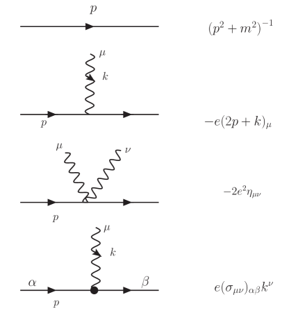
Figure 1: Feynman rules for spinor QED in the second-order formalism.

Of course the final results for physical amplitudes coincide with those of the better known first order formalism.

During the last two decades, these “string-inspired” representations have already found a considerable number of applications in QED, both for the calculation of photon amplitudes strassler1 ; 15 ; 51 and the effective action itself 5 ; cadhdu ; gussho1 ; gussho2 ; 95 . They have been generalised to include constant external fields shaisultanov ; 17 ; 18 ; 40 ; 51 ; 52 as well as finite temperature mckreb:therm1 ; mckreb:therm2 ; shovkovy:therm ; sato:therm ; mckeon:therm ; venwir . Their non-Abelian generalisation was used in the first calculation of the one-loop five-gluon amplitudes bediko5glu , a calculation of the non-Abelian heat-kernel coefficients to fifth order 25 , a calculation of the two-loop effective Lagrangian for a constant $SU(2)$ background field sascza , and very recently for obtaining gauge-invariant decompositions of the off-shell three- and four-gluon amplitudes 92 ; 105 ; 106 ; WI-qcd . In the non-Abelian case, it may be helpful to generate the particle color factor, and take care of the path ordering, by adding suitable auxiliary fields, in the same way as Grassmann variables take care of the spin factor and path ordering in (19) – see, for example, Balachandran:1976ya ; Barducci:1976xq ; Bastianelli:2013pta ; Ahmadiniaz:2015xoa . Further applications to QCD-related topics can be found in references Mueller:2017lzw ; Mueller:2017arw ; Mueller:2019qqj .

Extensions to curved space Bastianelli:2002fv and quantum gravity Bastianelli:2013tsa ; Bastianelli:2019xhi have also been considered, addressing in particular induced effective actions and graviton self-energies Bastianelli:2002qw ; Bastianelli:2005vk ; Bastianelli:2005uy , QED in curved spaces Hollowood:2007ku , gravitational corrections to the Euler-Heisenberg Lagrangians Bastianelli:2008cu ; Davila:2009vt and related amplitudes Bastianelli:2012bz , and studies of one-loop photon-graviton conversion in strong magnetic fields Bastianelli:2004zp ; Bastianelli:2007jv . The case of higher spin fields has also been approached using worldlines Bastianelli:2007pv ; Bastianelli:2008nm ; Corradini:2010ia ; Bastianelli:2012bn , as has quantum field theory on non-commutative spaces Bonezzi:2012vr ; Kiem:2001dm ; NCU1 ; NCUN and spaces with boundary Bastianelli:2006hq ; Bastianelli:2008vh ; ConfinedScalar .

However, with a few exceptions as in mckeon:ap224 ; mckreb:gamma ; mckshe ; karkto and Casalbuoni:1974pj ; Dai:2006vj ; Holzler:2007xt ; Dai:2008bh ; Bonezzi:2018box ; ahmadiniaz2020compton , these applications have been restricted to processes involving only closed scalar or spinor loops, not open lines. For the scalar QED case, Daikouji et al. dashsu have obtained the following master formula, analogous to (LABEL:scalarqedmaster), for the scalar propagator dressed with $N$ photons:

$$D^{p^{\prime}p}(k_{1},\varepsilon_{1};\cdots;k_{N},\varepsilon_{N}) = (-ie)^{N}(2\pi)^{D}\delta^{D}\Big{(}p+p^{\prime}+\sum_{i=1}^{N}k_{i}\Big{)}\int_{0}^{\infty}dT\,{\rm e}^{-m^{2}T}$$

$$\times\prod_{i=1}^{N}\int_{0}^{T}d\tau_{i}\,{\rm e}^{-Tb^{2}+\sum_{i,j=1}^{N}[\Delta_{ij}k_{i}\cdot k_{j}-2i{}^{\bullet}\!\Delta_{ij}\varepsilon_{i}\cdot k_{j}-{}^{\bullet}\!\Delta^{\hskip-1.42262pt\bullet}_{ij}\varepsilon_{i}\cdot\varepsilon_{j}]}\Big{|}_{\varepsilon_{1}\varepsilon_{2}\cdots\varepsilon_{N}}\,.$$

Here we have introduced the vector

$$b\equiv p^{\prime}+\frac{1}{T}\sum_{i=1}^{N}(k_{i}\tau_{i}-i\varepsilon_{i}),$$ (31)

and a different worldline Green’s function $\Delta(\tau,\tau^{\prime})$ has been used for the $q$ propagator:

$$\langle q^{\mu}(\tau)q^{\nu}(\tau^{\prime})\rangle = -2\Delta(\tau,\tau^{\prime})\delta^{\mu\nu},$$

$$\Delta(\tau,\tau^{\prime}) = \frac{|\tau-\tau^{\prime}|}{2}-\frac{\tau+\tau^{\prime}}{2}+\frac{\tau\tau^{\prime}}{T}\,.$$

Instead of the string-inspired boundary conditions (8), this Green’s function is adapted to Dirichlet boundary conditions,

$$q^{\mu}(0)=q^{\mu}(T)=0\,.$$ (33)

These boundary conditions break the translation invariance in proper-time, so that one now has to distinguish between derivatives with respect to the first and the second argument. A convenient notation is basvan-book to use left and right dots to indicate derivatives with respect to the first and the second argument, respectively:

$${}^{\bullet}\!\Delta(\tau,\tau^{\prime}) = \frac{\tau^{\prime}}{T}+\frac{1}{2}{\rm sign}(\tau-\tau^{\prime})-\frac{1}{2}\,,$$

$$\Delta^{\hskip-1.42262pt\bullet}(\tau,\tau^{\prime}) = \frac{\tau}{T}-\frac{1}{2}{\rm sign}(\tau-\tau^{\prime})-\frac{1}{2}\,,$$

$${}^{\bullet}\!\Delta^{\hskip-1.42262pt\bullet}(\tau,\tau^{\prime}) = \frac{1}{T}-\delta(\tau-\tau^{\prime})\,.$$

We will also need the coincidence limits

$$\Delta(\tau,\tau) = \frac{\tau^{2}}{T}-\tau\,;$$

$${}^{\bullet}\!\Delta(\tau,\tau) = \Delta^{\hskip-1.42262pt\bullet}(\tau,\tau)=\frac{\tau}{T}-{1\over 2}\,.$$

Note that, apart from the different boundary conditions, the Green’s functions $\Delta$ and $G_{B}$ differ also by a conventional factor of two in their normalisation. Finally, since $\Delta$ is somewhat less convenient than $G_{B}$, it is sometimes useful to observe that the two are related by

$$2\Delta(\tau,\tau^{\prime})=G_{B}(\tau,\tau^{\prime})-G_{B}(\tau,0)-G_{B}(0,\tau^{\prime})\,.$$ (36)

The master formula (LABEL:linemaster) represents the un-truncated dressed propagator, that is the sum of diagrams given in Fig. 2, where the final scalar propagators at each end are included. This technical point will play an important role in the following. The momenta $p,p^{\prime},k_{1},\ldots,k_{N}$ are all ingoing.

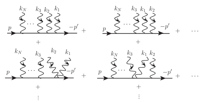
Figure 2: Multi-photon Compton scattering diagram in scalar QED (we do not distinguish the propagator of the matter field between scalar or spinor QED, choosing to indicate both with a solid line). The seagull vertices in the second row are once again produced by the $\delta$-function in the second derivative of the open-line Green function $\Delta$.

In dashsu it was obtained by a comparison with the Schwinger-parameter representation of the corresponding Feynman diagrams. The same formula has recently been rederived from the path integral representation (2) in 102 .

The worldline formalism has also been applied to the fermion line case mckreb:gamma ; karkto , but a Bern-Kosower type master formula for the dressed propagator has not been derived so far. The purpose of the present paper is to solve this long-standing problem, obtain such a formula, and to demonstrate its usefulness as an alternative to the standard Feynman diagram formalism. We will start from the well-known second-order representation of the $x$-space Dirac propagator $S^{x^{\prime}x}[A]$ in a Maxwell background,

$$S^{x^{\prime}x}[A] = \bigl{[}m+i\not{D}^{\prime}\bigr{]}K^{x^{\prime}x}[A]\,,$$ (37)

where $\not{D}=\gamma^{\mu}D_{\mu}$, $D_{\mu}=\partial_{\mu}+ieA_{\mu}$ and

$$K^{x^{\prime}x}[A] \equiv \Big{\langle}x^{\prime}\Big{|}\Bigl{[}m^{2}-D_{\mu}D^{\mu}+{i\over 2}\,e\gamma^{\mu}\gamma^{\nu}F_{\mu\nu}\Bigr{]}^{-1}\Big{|}x\Big{\rangle}\,.$$ (38)

For this “kernel” function, we will then derive the following path integral representation:

$$K^{x^{\prime}x}[A] = \int_{0}^{\infty}dT\,\,{\rm e}^{-m^{2}T}\,{\rm e}^{-{1\over 4}\frac{(x-x^{\prime})^{2}}{T}}\int_{q(0)=0}^{q(T)=0}Dq\,\,{\rm e}^{-\int_{0}^{T}d\tau\bigl{(}{1\over 4}\dot{q}^{2}+ie\,\dot{q}\cdot A+ie\frac{x^{\prime}-x}{T}\cdot A\bigr{)}}$$ (39)

$$\times\,2^{-\frac{D}{2}}{\rm symb}^{-1}\int_{\psi(0)+\psi(T)=0}D\psi\,\,{\rm e}^{-\int_{0}^{T}d\tau\,\bigl{[}{1\over 2}\psi_{\mu}\dot{\psi}^{\mu}-ieF_{\mu\nu}(\psi+\eta)^{\mu}(\psi+\eta)^{\nu}\bigl{]}}\,.$$

Here $\eta^{\mu}$ is an external Grassmann Lorentz vector, and the “symbol map,” symb, converts products of $\eta$’s into fully antisymmetrised products of Dirac matrices; we will discuss the details in section 3 below.

Following this we perform the usual projection onto an $N$-photon background, and use the path integral representation (39) to derive master formulas for the $N$ - photon kernel $K$ both in configuration and in momentum space. Those master formulas, given later in (LABEL:Ndressedmasterx) and (LABEL:Ndressedmasterp), are the central results of the paper.

Returning from the kernel $K$ to the propagator itself, we will then also Fourier transform our starting identity (37) to momentum space. Projected on the $N$-photon sector, it turns into

$$S_{N}^{p^{\prime}p}[\varepsilon_{1},k_{1};\ldots;\varepsilon_{N},k_{N}] = ({\not{p}^{\prime}}+m)K_{N}^{p^{\prime}p}[\varepsilon_{1},k_{1};\ldots;\varepsilon_{N},k_{N}]$$

$$-e\sum_{i=1}^{N}{\not{\varepsilon}_{i}}K_{(N-1)}^{p^{\prime}+k_{i},p}[\varepsilon_{1},k_{1};\ldots;\hat{\varepsilon}_{i},\hat{k}_{i};\ldots\varepsilon_{N},k_{N}]\,.$$

Here in the second term the ‘hat’ on $\varepsilon_{i}$ and $k_{i}$ means omission. We will work out this formula for $N=0,1,2$ to see how the equivalence to the standard formalism comes about in detail. As expected, the scalar QED calculations are close to the standard field theory ones, while in the fermion case nontrivial rearrangements have to be done to match the textbook Feynman diagram calculations.

The organisation of this paper, the first part in a series of three, is as follows: as a warm-up, in section 2 we shortly retrace the derivation of the scalar open line master formula (LABEL:scalarqedmasteropen) from the path integral representation (2), following 102 . In section 3 we derive the worldline path integral representation (39) of the kernel $K$ starting from field theory. Sections 4 and 5 contain the derivations of the configuration and momentum space master formulas, respectively. In section 6 we provide a different derivation of the $N$-photon kernel that keeps track of the orbital and spin contributions to the basic interaction between the electron and the photon in the underlying second-order formalism. We then move on from the $N$-photon kernel to the fully dressed electron propagator in section 7. We work out the cases $N=0,1,2$ and study the equivalence to the standard formalism, still off-shell, which happens in a quite non-obvious way. As a state-of-the-art application, in section 8 we recalculate the one-loop fermion self energy (in arbitrary dimension and covariant gauge). Section 9 offers our summary, and an outlook on future applications and generalisations.

There are four appendices: appendix A lists our conventions. Appendix B offers an alternative, more “principled,” derivation of the worldline path-integral representation of the electron propagator that, contrary to the one given in the main text, minimises the use of field theory concepts. Appendix C is devoted to the representation of the Feynman spin factor in terms of a Grassmann path integral. Finally, in D we prove a hypergeometric identity that we use in section 8 to simplify our result for the fermion self energy.

The forthcoming second part of this series will be devoted to the use of the master formulas derived here for on-shell calculations such as cross-sections, the third part to the inclusion of a constant electromagnetic background field.

2 The dressed propagator in scalar QED

In this section, we wish to derive the master formula, eventually given in (LABEL:scalarqedmasteropen), for the dressed propagator, and discuss some of its properties.

2.1 Derivation of the scalar master formula

Starting from (2), and proceeding as in the closed-loop case, we get a representation of this propagator in terms of the photon vertex operator (4) analogous to (LABEL:DNpointscal):

$$D_{N}^{x^{\prime}x}(k_{1},\varepsilon_{1};\cdots;k_{N},\varepsilon_{N}) = (-ie)^{N}\int_{0}^{\infty}dT\,{\rm e}^{-m^{2}T}\int_{x(0)=x}^{x(T)=x^{\prime}}Dx\,\,{\rm e}^{-\int_{0}^{T}d\tau{1\over 4}\dot{x}^{2}}$$

$$\times V_{\rm scal}[k_{1},\varepsilon_{1}]V_{\rm scal}[k_{2},\varepsilon_{2}]\cdots V_{\rm scal}[k_{N},\varepsilon_{N}]\,.$$

Shifting the path integration variable as

$$x(\tau)=x_{0}(\tau)+q(\tau)\,,$$ (42)

where $x_{0}$ is the straight-line trajectory

$$x_{0}(\tau)=x+(x^{\prime}-x)\frac{\tau}{T}\,,$$ (43)

reduces the boundary conditions to Dirichlet boundary conditions,

$$q(0)=q(T)=0\,.$$ (44)

Rewriting the photon vertex operator as in (9), (LABEL:linevertop) becomes

$$D_{N}^{x^{\prime}x}(k_{1},\varepsilon_{1};\cdots;k_{N},\varepsilon_{N}) = (-ie)^{N}\int_{0}^{\infty}dT\,{\rm e}^{-m^{2}T}\,{\rm e}^{-\frac{1}{4T}(x-x^{\prime})^{2}}\int_{q(0)=0}^{q(T)=0}Dq\,{\rm e}^{-\frac{1}{4}\int_{0}^{T}d\tau\,\dot{q}^{2}}$$

$$\times \prod_{i=1}^{N}\int_{0}^{T}d\tau_{i}\,{\rm e}^{\sum_{i=1}^{N}\big{(}\varepsilon_{i}\cdot\frac{(x^{\prime}-x)}{T}+\varepsilon_{i}\cdot\dot{q}(\tau_{i})+ik_{i}\cdot(x^{\prime}-x)\frac{\tau_{i}}{T}+ik_{i}\cdot x+ik_{i}\cdot q(\tau_{i})\big{)}}\Big{|}_{\varepsilon_{1}\varepsilon_{2}\cdots\varepsilon_{N}}\,.$$

The path integral can now be performed by formal Gaussian integration using the worldline Green function $\Delta(\tau,\tau^{\prime})$, leading to

$$D_{N}^{x^{\prime}x}(k_{1},\varepsilon_{1};\cdots;k_{N},\varepsilon_{N}) = (-ie)^{N}\int_{0}^{\infty}dT\,{\rm e}^{-m^{2}T}\,{\rm e}^{-\frac{1}{4T}(x-x^{\prime})^{2}}\big{(}4\pi T\big{)}^{-\frac{D}{2}}$$

$$\times\prod_{i=1}^{N}\int_{0}^{T}d\tau_{i}\,{\rm e}^{\sum_{i=1}^{N}\big{(}\varepsilon_{i}\cdot\frac{(x^{\prime}-x)}{T}+ik_{i}\cdot(x^{\prime}-x)\frac{\tau_{i}}{T}+ik_{i}\cdot x\big{)}}\,{\rm e}^{\sum_{i,j=1}^{N}\big{[}\Delta_{ij}k_{i}\cdot k_{j}-2i{}^{\bullet}\!\Delta_{ij}\varepsilon_{i}\cdot k_{j}-{}^{\bullet}\!\Delta^{\hskip-1.42262pt\bullet}_{ij}\varepsilon_{i}\cdot\varepsilon_{j}\big{]}}\Big{|}_{\varepsilon_{1}\varepsilon_{2}\cdots\varepsilon_{N}}\,.$$

(the free path integral normalisation (15) holds for Dirichlet boundary conditions as well). Finally, we also Fourier transform the scalar legs of the master formula in equation  (LABEL:bk-like-x) to momentum space:

$$D_{N}^{p^{\prime}p}(k_{1},\varepsilon_{1};\cdots;k_{N},\varepsilon_{N}) \equiv \int d^{D}x\int d^{D}x^{\prime}\,{\rm e}^{ip\cdot x+ip^{\prime}\cdot x^{\prime}}\,D^{x^{\prime}x}(k_{1},\varepsilon_{1};\cdots;k_{N},\varepsilon_{N})\,.$$ (47)

After a change of variables from $x,x^{\prime}$ to $x_{\pm}$, defined by

$$x_{+} = \frac{1}{2}(x+x^{\prime})\,,$$

$$x_{-} = x^{\prime}-x\,,$$

the integral over $x_{+}$ produces the delta-function for the total conservation of energy-momentum:

$$D_{N}^{p^{\prime}p}(k_{1},\varepsilon_{1};\cdots;k_{N},\varepsilon_{N}) = (-ie)^{N}(2\pi)^{D}\delta^{D}\Big{(}p+p^{\prime}+\sum_{i=1}^{N}k_{i}\Big{)}\int_{0}^{\infty}dT\,{\rm e}^{-m^{2}T}(4\pi T)^{-\frac{D}{2}}\int d^{D}x_{-}\,{\rm e}^{-\frac{1}{4T}x_{-}^{2}}$$

$$\times\prod_{i=1}^{N}\int_{0}^{T}d\tau_{i}\,{\rm e}^{ix_{-}\cdot\big{(}p^{\prime}+\frac{1}{T}\sum_{i=1}^{N}(k_{i}\tau_{i}-i\varepsilon_{i})\big{)}}\,{\rm e}^{\sum_{i,j=1}^{N}\big{[}\Delta_{ij}k_{i}\cdot k_{j}-2i{}^{\bullet}\!\Delta_{ij}\varepsilon_{i}\cdot k_{j}-{}^{\bullet}\!\Delta^{\hskip-1.42262pt\bullet}_{ij}\varepsilon_{i}\cdot\varepsilon_{j}\big{]}}\Big{|}_{\varepsilon_{1}\varepsilon_{2}\cdots\varepsilon_{N}}\,.$$

Performing also the $x_{-}$ integral, one arrives at the momentum space master formula given in the introduction, (LABEL:linemaster).

Let us also introduce some more notation here. The result of expanding out the exponential factor in (LABEL:linemaster) will be named $(-i)^{N}\bar{P}_{N}\,\,{\rm e}^{(\cdot)}$, namely

$$(-i)^{N}\bar{P}_{N}\,\,{\rm e}^{(\cdot)}={\rm e}^{-Tb^{2}+\sum_{i,j=1}^{N}\big{[}\Delta_{ij}k_{i}\cdot k_{j}-2i{}^{\bullet}\!\Delta_{ij}\varepsilon_{i}\cdot k_{j}-{}^{\bullet}\!\Delta^{\hskip-1.42262pt\bullet}_{ij}\varepsilon_{i}\cdot\varepsilon_{j}\big{]}}\Big{|}_{\varepsilon_{1}\varepsilon_{2}\cdots\varepsilon_{N}}\,,$$

where now

$$\,{\rm e}^{(\cdot)}\equiv{\rm e}^{-Tb_{0}^{2}+\sum_{i,j=1}^{N}\Delta_{ij}k_{i}\cdot k_{j}}\,,$$ (51)

and

$$b_{0}\equiv b|_{\varepsilon_{1}=\cdots=\varepsilon_{N}=0}=p^{\prime}+\frac{1}{T}\sum_{i=1}^{N}k_{i}\tau_{i}$$ (52)

(the ‘bar’ on $P_{N}$ is to distinguish it from the corresponding quantity for the closed loop 41 ).

2.2 Off-shell IBP

One of the advantages of this master formula’s encoding of the usual Feynman-parameter integrals in terms of the worldline Green function $\Delta$ is that IBP can be used to remove the second derivative ${}^{\bullet}\!\Delta^{\hskip-1.42262pt\bullet}$, and thus the seagull vertex. This homogenises the integrand and leads to the automatic appearance of field strength tensors, which again can be arranged into bi-cycles. Those now take the form (compare (18))

$${}^{\bullet}\!\Delta(i_{1}i_{2}\ldots i_{n})\equiv{}^{\bullet}\!\Delta_{i_{1}i_{2}}{}^{\bullet}\!\Delta_{i_{2}i_{3}}\cdots{}^{\bullet}\!\Delta_{i_{n}i_{1}}Z_{n}(i_{1}i_{2}\ldots i_{n})\quad(n\geq 2)\,.$$ (53)

The same IBP algorithm as in the closed-loop case 26 ; 41 can be used, and non-vanishing boundary terms are still not generated due to $\Delta(\tau,\tau^{\prime})$ obeying Dirichlet boundary conditions. The resulting integrand will be called $(-i)^{N}\bar{Q}_{N}\,\,{\rm e}^{(\cdot)}$. $\bar{Q}_{N}$ in general will contain both $\Delta^{\hskip-1.42262pt\bullet}(\tau,\tau^{\prime})$ and ${}^{\bullet}\!\Delta(\tau,\tau^{\prime})$, but we will standardise it using the identity $\Delta^{\hskip-1.42262pt\bullet}(\tau,\tau^{\prime})={}^{\bullet}\!\Delta(\tau^{\prime},\tau)$ to trade the former for the latter throughout.

We will call this IBP algorithm “Off-shell IBP” because it is designed not to generate any boundary terms. Below we will define an alternative IBP procedure that seems preferable in the on-shell case.

Let us work out the integrand for $N=1,2$. For $N=1$, the expansion of the exponential factor in (LABEL:linemaster) yields

$${\bar{P}_{1}} = 2{}^{\bullet}\!\Delta_{11}\varepsilon_{1}\cdot k_{1}-2\varepsilon_{1}\cdot b_{0}\,.$$

Here there are no second derivatives yet, so $\bar{Q}_{1}=\bar{P}_{1}$.

For $N=2$ we find

$${\bar{P}}_{2} = 4({}^{\bullet}\!\Delta_{12}\varepsilon_{1}\cdot k_{2}+{}^{\bullet}\!\Delta_{11}\varepsilon_{1}\cdot k_{1}-\varepsilon_{1}\cdot b_{0})({}^{\bullet}\!\Delta_{21}\varepsilon_{2}\cdot k_{1}+{}^{\bullet}\!\Delta_{22}\varepsilon_{2}\cdot k_{2}-\varepsilon_{2}\cdot b_{0})$$ (55)

$$-\bigl{(}\frac{2}{T}-2{}^{\bullet}\!\Delta^{\hskip-1.42262pt\bullet}_{12}\bigr{)}\varepsilon_{1}\cdot\varepsilon_{2}\,.$$

Here the last term asks for IBP, which transforms it as

$$2{}^{\bullet}\!\Delta^{\hskip-1.42262pt\bullet}_{12}\varepsilon_{1}\cdot\varepsilon_{2}\longrightarrow - \Bigl{(}4{}^{\bullet}\!\Delta_{12}{}^{\bullet}\!\Delta_{21}k_{1}\cdot k_{2}+2{}^{\bullet}\!\Delta_{11}{}^{\bullet}\!\Delta_{21}k_{1}^{2}+2{}^{\bullet}\!\Delta_{12}{}^{\bullet}\!\Delta_{22}k_{2}^{2}-2{}^{\bullet}\!\Delta_{12}k_{2}\cdot b_{0}$$

$$-2{}^{\bullet}\!\Delta_{21}k_{1}\cdot b_{0}\Bigr{)}\varepsilon_{1}\cdot\varepsilon_{2}\,,$$

where we have used the identity ${\partial\over\partial\tau_{i}}\Delta_{ii}=2{}^{\bullet}\!\Delta_{ii}$. Sorting according to cycles, ${\bar{Q}}_{2}$ can be written as

$${\bar{Q}}_{2} = 4{}^{\bullet}\!\Delta(12)+4{}^{\bullet}\!\Delta_{12}\varepsilon_{1}\cdot k_{2}({}^{\bullet}\!\Delta(2)-\varepsilon_{2}\cdot b_{0})+4({}^{\bullet}\!\Delta(1)-\varepsilon_{1}\cdot b_{0}){}^{\bullet}\!\Delta_{21}\varepsilon_{2}\cdot k_{1}$$

$$+4({}^{\bullet}\!\Delta(1)-\varepsilon_{1}\cdot b_{0})({}^{\bullet}\!\Delta(2)-\varepsilon_{2}\cdot b_{0})$$

$$-\Bigl{(}\frac{2}{T}+2{}^{\bullet}\!\Delta_{11}{}^{\bullet}\!\Delta_{21}k_{1}^{2}+2{}^{\bullet}\!\Delta_{12}{}^{\bullet}\!\Delta_{22}k_{2}^{2}-2{}^{\bullet}\!\Delta_{12}k_{2}\cdot b_{0}-2{}^{\bullet}\!\Delta_{21}k_{1}\cdot b_{0}\Bigr{)}\varepsilon_{1}\cdot\varepsilon_{2}\,.$$

where we used the following compact notation

$${}^{\bullet}\!\Delta(i)\equiv{}^{\bullet}\!\Delta_{ii}\varepsilon_{i}\cdot k_{i}.$$

2.3 The QED Ward identity

The amplitude $D_{N}^{p^{\prime}p}(k_{1},\varepsilon_{1};\cdots;k_{N},\varepsilon_{N})$ should fulfill the QED Ward identity, i.e. replacing any

$$\varepsilon_{i}\to k_{i}$$ (58)

should give something that does not contribute on-shell. This property is not obvious from the master formulas (LABEL:e1) or (LABEL:linemaster), but is easily seen in the path-integral representation (LABEL:linevertop). The replacement (58) turns the vertex operator $V_{\rm scal}[k_{i},\varepsilon_{i}]$ into

$$V_{\rm scal}[k_{i},k_{i}]=\frac{1}{i}\int_{0}^{T}d\tau_{i}\frac{d}{d\tau_{i}}\,{\rm e}^{ik_{i}\cdot x(\tau)}=-i(\,{\rm e}^{ik_{i}\cdot x(T)}-\,{\rm e}^{ik_{i}\cdot x(0)})=-i(\,{\rm e}^{ik_{i}\cdot x^{\prime}}-\,{\rm e}^{ik_{i}\cdot x})\,.$$

Under the Fourier transformation (47), the first term in brackets will change the denominator of the right-most scalar propagator (in the conventions of fig. 2) from $p^{\prime 2}+m^{2}$ to $(p^{\prime}+k_{i})^{2}+m^{2}$, while the second term changes the denominator of the left-most scalar propagator from $p^{2}+m^{2}$ to $(p+k_{i})^{2}+m^{2}$. Thus neither term conserves the double pole that by the LSZ theorem is necessary for contributing to the on-shell matrix element.

We can take advantage of the Ward identity to achieve manifest gauge invariance at the integrand level. Namely, let us choose for each $k_{i}$ a “reference vector” $r_{i}$ such that $k_{i}\cdot r_{i}\neq 0$, and define the modified vertex operator

$$V_{\rm scal}[k,\varepsilon,r] \equiv V_{\rm scal}[k,\varepsilon]+i\frac{\varepsilon\cdot r}{k\cdot r}\int_{0}^{T}d\tau\frac{d}{d\tau}\,{\rm e}^{ik\cdot x(\tau)}$$ (60)

$$= \int_{0}^{T}d\tau\frac{r\cdot f\cdot{\dot{x}}}{r\cdot k}\,{\rm e}^{ik\cdot x(\tau)}=\int_{0}^{T}d\tau\,{\rm e}^{ik\cdot x(\tau)+\frac{r\cdot f\cdot{\dot{x}}}{r\cdot k}}\Big{|}_{f}\,.$$

Plugging this back into (LABEL:linevertop) and Fourier transforming to momentum space the on-shell version of the master formula for the dressed propagator in terms of the field strength tensors is given by

$$\mathcal{M}^{p^{\prime}p}(k_{1},f_{1};\cdots k_{N},f_{N})\equiv(p^{\prime 2}+m^{2})D_{N}^{p^{\prime}p}(k_{1},f_{1};\cdots;k_{N},f_{N})(p^{2}+m^{2})$$

$$=(-ie)^{N}(2\pi)^{D}\delta^{D}\Big{(}p+p^{\prime}+\sum_{i=1}^{N}k_{i}\Big{)}\int_{0}^{\infty}dT\,{\rm e}^{-m^{2}T}(4\pi T)^{-\frac{D}{2}}\int d^{D}x_{-}\,{\rm e}^{-\frac{1}{4T}x_{-}^{2}}$$

$$\times\prod_{i=1}^{N}\int_{0}^{T}d\tau_{i}\,{\rm e}^{ix_{-}\cdot\big{(}p^{\prime}+\frac{1}{T}\sum_{i=1}^{N}(k_{i}\tau_{i}+i\frac{f_{i}\cdot r_{i}}{r_{i}\cdot k_{i}})\big{)}}\,{\rm e}^{\sum_{i,j=1}^{N}\big{[}\Delta_{ij}k_{i}\cdot k_{j}-2i{}^{\bullet}\!\Delta_{ij}\frac{r_{i}\cdot f_{i}\cdot k_{j}}{r_{i}\cdot k_{i}}-{}^{\bullet}\!\Delta^{\hskip-1.42262pt\bullet}_{ij}\frac{r_{i}\cdot f_{i}\cdot f_{j}\cdot r_{j}}{r_{i}\cdot k_{i}\,r_{j}\cdot k_{j}}\big{]}}\Big{|}_{f_{1}f_{2}\cdots f_{N}}\,,$$

(61)

which will be discussed more in the forthcoming paper. Retracing the derivation of the master formula (LABEL:scalarqedmaster) with this modified vertex operator, we arrive at the “covariantised Bern-Kosower master formula” (henceforth we usually omit the global energy-momentum conservation factor)

$$\Gamma_{\rm scal}[k_{1},\varepsilon_{1};\ldots;k_{N},\varepsilon_{N}] = {(-ie)}^{N}{\displaystyle\int_{0}^{\infty}}{dT\over T}{(4\pi T)}^{-{D\over 2}}\,{\rm e}^{-m^{2}T}\prod_{i=1}^{N}\int_{0}^{T}d\tau_{i}$$

$$\times\exp\biggl{\{}\sum_{i,j=1}^{N}\Bigl{[}{1\over 2}G_{Bij}k_{i}\cdot k_{j}-i\dot{G}_{Bij}{r_{i}\cdot f_{i}\cdot k_{j}\over r_{i}\cdot k_{i}}-{1\over 2}\ddot{G}_{Bij}{r_{i}\cdot f_{i}\cdot f_{j}\cdot r_{j}\over r_{i}\cdot k_{i}\,r_{j}\cdot k_{j}}\Bigr{]}\biggr{\}}\Bigg{|}_{f_{1}f_{2}\ldots f_{N}}\,.$$

(62)

In 91 this version of the master formula was obtained by IBP at the parameter integral level and called the “R-representation.” Note that it reduces to the original master formula (LABEL:scalarqedmaster) if $r_{i}\cdot\varepsilon_{i}=0$ for all $i$.

2.4 Alternative forms of the master formula

Finally, let us also give two alternative forms of the master formula (LABEL:linemaster). Writing the worldline Green function explicitly, and taking advantage of some cancellations in the exponent, one can rewrite it as

$$D_{N}^{p^{\prime}p}(k_{1},\varepsilon_{1};\cdots;k_{N},\varepsilon_{N})=(-ie)^{N}\int_{0}^{\infty}dT\,{\rm e}^{-T(m^{2}+p^{\prime 2})}$$

$$\times \int_{0}^{T}\prod_{i=1}^{N}d\tau_{i}\,{\rm e}^{\sum_{i=1}^{N}(-2k_{i}\cdot p^{\prime}\tau_{i}+2i\varepsilon_{i}\cdot p^{\prime})+\sum_{i,j=1}^{N}\big{[}\bigl{(}\frac{|\tau_{i}-\tau_{j}|}{2}-\frac{\tau_{i}+\tau_{j}}{2}\bigr{)}k_{i}\cdot k_{j}-i({\rm sign}(\tau_{i}-\tau_{j})-1)\varepsilon_{i}\cdot k_{j}+\delta(\tau_{i}-\tau_{j})\varepsilon_{i}\cdot\varepsilon_{j}\big{]}}\Big{|}_{\varepsilon_{1}\varepsilon_{2}\cdots\varepsilon_{N}}\,.$$

And this can be written even more compactly at the expense of introducing some more notation. Namely, defining

$$k_{0} \equiv p^{\prime}\,,\quad k_{N+1}\equiv p\,,\quad\tau_{0}\equiv T\,,\quad\tau_{N+1}\equiv 0\,,\quad\varepsilon_{0}\equiv 0\,,\quad\varepsilon_{N+1}\equiv 0\,,$$

we can, using energy-momentum conservation in the exponent, arrive at the following form:

$$D_{N}^{p^{\prime}p}(k_{1},\varepsilon_{1};\cdots;k_{N},\varepsilon_{N}) = (-ie)^{N}\int_{0}^{\infty}dT\,{\rm e}^{-m^{2}T}$$

$$\times \int_{0}^{T}\prod_{i=1}^{N}d\tau_{i}\,{\rm e}^{\sum_{i,j=0}^{N+1}\big{[}\frac{1}{2}|\tau_{i}-\tau_{j}|k_{i}\cdot k_{j}-i{\rm sign}(\tau_{i}-\tau_{j})\varepsilon_{i}\cdot k_{j}+\delta(\tau_{i}-\tau_{j})\varepsilon_{i}\cdot\varepsilon_{j}\big{]}}\Big{|}_{\varepsilon_{1}\varepsilon_{2}\cdots\varepsilon_{N}}\,.$$

It is this form of the momentum space master formula that was previously obtained by Daikouji et al. dashsu by a direct comparison with the corresponding Feynman-Schwinger parameter integrals and later in 102 using the worldline formalism. It turns out that the above formula has the advantage of leading to manifest worldline Poincarè invariance on the mass-shell of the scalar particle Ahmadiniaz:2015xoa . This provides a worldline analogue of the well-known fact that in string theory the worldsheet theory becomes conformally invariant only if all vertex operator insertions are on-shell.

3 Path integral representation of the electron propagator in an Abelian background field

Contrary to the scalar case, there are various routes to obtain a worldline path integral representation of the fermion propagator in a Maxwell background. In this section, we will present a field-theory based construction that essentially follows fragit , delegating some technical details to appendix C. The same representation is rederived in appendix B from an intrinsic worldline point of view.

The most specific feature of the method presented here, is the use of “Weyl symbols”, defined in (71) below, to represent fermionic operators bermar ; hentei-book . See bc ; hht ; holten ; bhattacharya for the alternative “holomorphic representation.”

We look for a path integral representation of

$$S^{x^{\prime}x}[A] = =\big{\langle}x^{\prime}\big{|}{\bigl{[}m-i\not{D}\bigr{]}}^{-1}\big{|}x\big{\rangle}=\big{\langle}x^{\prime}\big{|}{\bigl{[}m-i\not{\partial}+e\not{A}\bigr{]}}^{-1}\big{|}x\big{\rangle}=\big{\langle}x^{\prime}\big{|}{\bigl{[}m+\not{p}+e\not{A}\bigr{]}}^{-1}\big{|}x\big{\rangle}\,.$$

We start with using the Gordon identity

$${\not{D}}^{2}=-D_{\mu}D^{\mu}+{i\over 2}\,e\gamma^{\mu}\gamma^{\nu}F_{\mu\nu}\,,$$ (67)

to rewrite

$${\bigl{[}m-i\not{D}\bigr{]}}^{-1} = \bigl{[}m+i\not{D}\bigr{]}\bigl{[}m+i\not{D}\bigr{]}^{-1}{\bigl{[}m-i\not{D}\bigr{]}}^{-1}$$

$$= \Bigl{[}m+i\not{D}\Bigr{]}\Bigl{[}m^{2}-D_{\mu}D^{\mu}+{i\over 2}\,e\gamma^{\mu}\gamma^{\nu}F_{\mu\nu}\Bigr{]}^{-1}\,.$$

This brings us to the formulas defining the second-order representation that we already quoted in the introduction, (37) and (38). The kernel $K^{x^{\prime}x}[A]$ is formally identical with the propagator for a scalar particle in the background containing the gauge field $A$ and the matrix-valued potential $V={i\over 2}\,e\gamma^{\mu}\gamma^{\nu}F_{\mu\nu}$. It is thus straightforward to obtain the following path integral representation for it (see, e.g., 41 )

$$K^{x^{\prime}x}[A] = \int_{0}^{\infty}dT\,\,{\rm e}^{-m^{2}T}\int_{x(0)=x}^{x(T)=x^{\prime}}Dx\,{\cal P}\,{\rm e}^{-\int_{0}^{T}d\tau\bigl{(}{1\over 4}\dot{x}^{2}+ie\,\dot{x}\cdot A+{i\over 2}\,e\gamma^{\mu}\gamma^{\nu}F_{\mu\nu}\bigr{)}}\,,$$ (69)

which generalises (6) to the open-line case. We now wish to remove the path-ordering $\cal P$. This requires an identity like the one we used for the closed-loop case, (19), but without taking the trace. As we show in appendix C, this identity is

$${\cal P}e^{-\int_{0}^{T}d\tau{i\over 2}\,eF_{\mu\nu}\gamma^{\mu}\gamma^{\nu}}=2^{-\frac{D}{2}}{\rm symb}^{-1}\int_{A}D\psi\,\,{\rm e}^{-\int_{0}^{T}d\tau\,\bigl{[}{1\over 2}\psi_{\mu}\dot{\psi}^{\mu}-ieF_{\mu\nu}(\psi+\eta)^{\mu}(\psi+\eta)^{\nu}\bigl{]}}\,.$$ (70)

Here the symbol map, symb, is defined by

$${\rm symb}\bigl{(}\gamma^{\alpha_{1}\alpha_{2}\cdots\alpha_{n}}\bigr{)}\equiv(-i\sqrt{2})^{n}\eta^{\alpha_{1}}\eta^{\alpha_{2}}\ldots\eta^{\alpha_{n}}\,,$$ (71)

where $\gamma^{\alpha\beta\cdots\rho}$ denotes the totally antisymmetrised product of gamma matrices:

$$\gamma^{\alpha_{1}\alpha_{2}\cdots\alpha_{n}}\equiv\frac{1}{n!}\sum_{\pi\in S_{n}}{\rm sign}(\pi)\gamma^{\alpha_{\pi(1)}}\gamma^{\alpha_{\pi(2)}}\cdots\gamma^{\alpha_{\pi(n)}}\,.$$ (72)

Note that in $D$ dimensions the right-hand of (71) side will vanish for more than $D$ factors by the Grassmann property of the $\eta^{\alpha}$.

Putting the pieces together, we arrive at our final path integral representation for the kernel as given in the introduction, equation (39). Together with (37) it is a suitable starting point for calculating the fermionic propagator $S^{x^{\prime}x}[A]$ in the string-inspired formalism.

4 Master formula for the $N$ - photon kernel in $x$ - space

Choosing $A(x)$ as a sum of $N$ plane waves with polarisation vectors $\varepsilon_{i}^{\mu}$ and wave vectors $k_{i}^{\mu}$ as in (39), and keeping only the terms containing each polarisation vector linearly, we get the “$N$-photon dressed” version of the kernel $K^{x^{\prime}x}$:

$$K^{x^{\prime}x}_{N}(k_{1},\varepsilon_{1};\ldots;k_{N},\varepsilon_{N}) = (-ie)^{N}2^{-\frac{D}{2}}\int_{0}^{\infty}dT\,\,{\rm e}^{-m^{2}T}\,{\rm e}^{-{1\over 4}\frac{(x-x^{\prime})^{2}}{T}}\int_{q(0)=0}^{q(T)=0}Dq\,\,{\rm e}^{-\int_{0}^{T}d\tau\frac{\dot{q}^{2}}{4}}$$

$$\times{\rm symb}^{-1}\int_{\psi(0)+\psi(T)=0}D\psi\,\,{\rm e}^{-\int_{0}^{T}d\tau\,{1\over 2}\psi\dot{\psi}}\,V^{x^{\prime}x}_{\eta}[k_{1},\varepsilon_{1}]\cdots V^{x^{\prime}x}_{\eta}[k_{N},\varepsilon_{N}]\,.$$

Here $V^{x^{\prime}x}_{\eta}[k,\varepsilon]$ is the photon vertex operator for the open line, which now reads

$$V^{x^{\prime}x}_{\eta}[k,\varepsilon]=\int_{0}^{T}d\tau\biggl{[}\varepsilon\cdot\Bigl{(}\frac{x^{\prime}-x}{T}+\dot{q}\Bigr{)}+2i\varepsilon\cdot\bigl{(}\psi+\eta\bigr{)}k\cdot\bigl{(}\psi+\eta\bigr{)}\biggr{]}\,{\rm e}^{ik\cdot\bigl{(}x+(x^{\prime}-x)\frac{\tau}{T}+q(\tau)\bigr{)}}\,.$$

(74)

We could now do the double path integral as it stands, using the Green functions $G_{B}$ and $G_{F}$ and standard Gaussian combinatorics. However, if we aim at a closed-form expression valid for any $N$, it will be necessary to find a suitable extension of the exponentiation formula (9) to the fermionic case. As we explained already in the introduction for the closed-loop case, an elegant way to achieve this is though the introduction of $N=1$ worldline superspace, as motivated by the underlying worldline supersymmetry (LABEL:susy). Thus, introducing the worldline superfield

$$Q^{\mu}(\tau)\equiv q^{\mu}(\tau)+\sqrt{2}\,\theta\psi^{\mu}(\tau)\,,$$ (75)

and using the superspace conventions introduced in the introduction, we can rewrite the vertex operator (74) in the form

$$V^{x^{\prime}x}_{\eta}[k,\varepsilon]=\int_{0}^{T}d\tau\int d\theta\,\varepsilon\cdot\biggl{[}-\theta\,\frac{x^{\prime}-x}{T}+\sqrt{2}\eta+DQ\biggr{]}\,{\rm e}^{ik\cdot\bigl{[}x+(x^{\prime}-x)\frac{\tau}{T}+\sqrt{2}\theta\eta+Q(\tau)\bigr{]}}\,.$$

(76)

Recall that for the time being we must also treat the polarisation vectors $\varepsilon_{i}$ as Grassmann variables. After the usual formal exponentiation of the prefactor, we obtain the required purely exponential form of the vertex operator:

$$V^{x^{\prime}x}_{\eta}[k,\varepsilon]=\int_{0}^{T}d\tau\int d\theta\,{\rm e}^{ik\cdot x+\frac{x^{\prime}-x}{T}(\theta\varepsilon+i\tau k)-\sqrt{2}\eta\cdot(\varepsilon+i\theta k)+\varepsilon\cdot DQ+ik\cdot Q}\Big{|}_{\varepsilon}\,.$$ (77)

Thus the path integral is ready for evaluation by completion of the square, which yields the following Bern-Kosower type master formula for the $N$-photon kernel in $x$-space:

$$K^{x^{\prime}x}_{N}(k_{1},\varepsilon_{1};\ldots;k_{N},\varepsilon_{N}) = (-ie)^{N}{\rm symb}^{-1}\int_{0}^{\infty}\frac{dT}{(4\pi T)^{\frac{D}{2}}}\,{\rm e}^{-m^{2}T}\,{\rm e}^{-{1\over 4}\frac{(x-x^{\prime})^{2}}{T}}\int_{0}^{T}d\tau_{1}\cdots\int d\theta_{N}$$

$$\times\,{\rm e}^{\sum_{i=1}^{N}\bigl{[}ik_{i}\cdot x+\frac{x^{\prime}-x}{T}(\theta_{i}\varepsilon_{i}+i\tau_{i}k_{i})-\sqrt{2}\eta\cdot(\varepsilon_{i}+i\theta_{i}k_{i})\bigr{]}+\sum_{i,j=1}^{N}\bigl{[}\hat{\Delta}_{ij}k_{i}\cdot k_{j}+2iD_{i}\hat{\Delta}_{ij}\varepsilon_{i}\cdot k_{j}+D_{i}D_{j}\hat{\Delta}_{ij}\varepsilon_{i}\cdot\varepsilon_{j}\bigr{]}}\Big{|}_{\varepsilon_{1}\varepsilon_{2}\cdots\varepsilon_{N}}\,.$$

Here $\hat{\Delta}$ is now the super worldline Green’s function appropriate for the combination of Dirichlet and antiperiodic boundary conditions at hand:

$$\hat{\Delta}(\tau,\theta;\tau^{\prime},\theta^{\prime})\equiv\Delta(\tau,\tau^{\prime})+{1\over 2}\theta\theta^{\prime}G_{F}(\tau,\tau^{\prime})\,.$$ (79)

Let us also write explicitly the derivatives of this Green’s function that appear in the master formulas:

$$D_{i}\hat{\Delta}_{ij} = {1\over 2}\theta_{j}G_{Fij}-\theta_{i}{}^{\bullet}\!\Delta_{ij}\,;$$

$$D_{j}\hat{\Delta}_{ij} = -{1\over 2}\theta_{i}G_{Fij}-\theta_{j}\Delta^{\hskip-1.42262pt\bullet}_{ij}\,;$$

$$D_{i}D_{j}\hat{\Delta}_{ij} = -{1\over 2}G_{Fij}+\theta_{i}\theta_{j}{}^{\bullet}\!\Delta^{\hskip-1.42262pt\bullet}_{ij}$$

(no summation convention).

5 Master formula for the $N$ - photon kernel in momentum space

In the following we give the momentum space version of the master formula derived above. We eventually specialise to $D=4$ and work out the explicit form of the kernel for some simple cases.

5.1 The master formula

We begin by Fourier transforming the master formula (LABEL:Ndressedmasterx) to momentum space,

$$K^{p^{\prime}p}_{N}(k_{1},\varepsilon_{1};\ldots;k_{N},\varepsilon_{N}) = \int d^{D}x\int d^{D}x^{\prime}\,{\rm e}^{ip\cdot x+ip^{\prime}\cdot x^{\prime}}\,K^{x^{\prime}x}_{N}(k_{1},\varepsilon_{1};\ldots;k_{N},\varepsilon_{N})\,.$$ (81)

After a change of variables from $x$, $x^{\prime}$ to $x_{\pm}$ as in (LABEL:cov), the $x_{+}$ - integral produces the global momentum conservation factor $(2\pi)^{D}\delta^{D}(p+p^{\prime}+\sum_{i=1}^{N}k_{i})$, which we omit in the following. The $x_{-}$ - integral can, using momentum conservation, be written as

$$\int d^{D}x_{-}\,{\rm e}^{-{1\over 4}\frac{x_{-}^{2}}{T}+\bigl{[}ip^{\prime}+\frac{1}{T}\sum_{i=1}^{N}(\theta_{i}\varepsilon_{i}+i\tau_{i}k_{i})\bigr{]}\cdot x_{-}}=(4\pi T)^{\frac{D}{2}}\,{\rm e}^{T\bigl{[}ip^{\prime}+\frac{1}{T}\sum_{i=1}^{N}(\theta_{i}\varepsilon_{i}+i\tau_{i}k_{i})\bigr{]}^{2}}\,.$$ (82)

This brings us to

$$K^{p^{\prime}p}_{N}(k_{1},\varepsilon_{1};\ldots;k_{N},\varepsilon_{N}) = (-ie)^{N}{\rm symb}^{-1}\int_{0}^{\infty}dT\,{\rm e}^{-m^{2}T}\int_{0}^{T}d\tau_{1}\cdots\int d\theta_{N}\,\,{\rm e}^{\rm Exp}\Big{|}_{\varepsilon_{1}\varepsilon_{2}\cdots\varepsilon_{N}}\,,$$

where

$${\rm Exp} = T\bigl{[}ip^{\prime}+\frac{1}{T}\sum_{i=1}^{N}(\theta_{i}\varepsilon_{i}+i\tau_{i}k_{i})\bigr{]}^{2}-\sum_{i=1}^{N}\sqrt{2}\eta\cdot(\varepsilon_{i}+i\theta_{i}k_{i})$$

$$+\sum_{i,j=1}^{N}\bigl{[}\hat{\Delta}_{ij}k_{i}\cdot k_{j}+2iD_{i}\hat{\Delta}_{ij}\varepsilon_{i}\cdot k_{j}+D_{i}D_{j}\hat{\Delta}_{ij}\varepsilon_{i}\cdot\varepsilon_{j}\bigr{]}\,.$$

Using (LABEL:Dformulas),(LABEL:derDelta) and momentum conservation, this can be written explicitly as (in the following we often abbreviate ${\rm sign}(\tau_{i}-\tau_{j})$ by $\sigma_{ij}$ and $\delta\left(\tau_{i}-\tau_{j}\right)$ by $\delta_{ij}$)

$${\rm Exp} = -p^{\prime 2}T-\sum_{i=1}^{N}\sqrt{2}{\eta}\cdot(\varepsilon_{i}+i\theta_{i}k_{i})+{1\over 2}\sum_{i,j=1}^{N}\theta_{i}\theta_{j}\sigma_{ij}k_{i}\cdot k_{j}$$ (85)

$$+\sum_{i=1}^{N}(i\theta_{i}\varepsilon_{i}-\tau_{i}k_{i})\cdot\bigl{(}p^{\prime}-p-\sum_{j=1}^{N}\sigma_{ij}k_{j}\bigr{)}-i\sum_{i,j=1}^{N}\sigma_{ij}\varepsilon_{i}\cdot k_{j}\theta_{j}$$

$$-{1\over 2}\sum_{i,j=1}^{N}\bigl{(}\sigma_{ij}+2\theta_{i}\theta_{j}\delta_{ij}\bigr{)}\varepsilon_{i}\cdot\varepsilon_{j}\,.$$

This appears to be the most useful form of writing the exponent of the momentum-space master formula. Nevertheless, let us mention in passing that there is also a suggestive form of the exponent that generalises (LABEL:master-dss). There we found that, in the scalar case, with the additional definitions (LABEL:defKextension) the exponent can be rewritten purely in terms of the functions $|\tau_{i}-\tau_{j}|$, ${\rm sign}(\tau_{i}-\tau_{j})$ and $\delta(\tau_{i}-\tau_{j})$, that is, in terms of the Green’s function for the second derivative on the line

$$g(\tau,\tau^{\prime})\equiv{1\over 2}|\tau-\tau^{\prime}|\,,$$ (86)

and its derivatives. Worldline supersymmetry then leads one to suspect that, in spinor QED, a similar rewriting should be possible in terms of the supersymmetric generalisation of this Green’s function, and its super-derivatives. This Green function can be given in terms of the super-distance on the line, $|\tau-\tau^{\prime}|+\theta\theta^{\prime}{\rm sign}(\tau-\tau^{\prime})$, as (see, e.g., polyakovbook ; MeContact ):

$$\hskip 3.00003pt\widehat{g}\hskip 3.99994pt(\tau,\theta;\tau^{\prime},\theta^{\prime}) \equiv {1\over 2}(|\tau-\tau^{\prime}|+\theta\theta^{\prime}{\rm sign}(\tau-\tau^{\prime}))\,$$ (87)

so that

$$D_{i}\,\hskip 3.00003pt\widehat{g}\hskip 3.99994pt_{ij} = -{1\over 2}(\theta_{i}-\theta_{j})\sigma_{ij}$$

$$D_{i}D_{j}\,\hskip 3.00003pt\widehat{g}\hskip 3.99994pt_{ij} = -{1\over 2}(\sigma_{ij}+2\theta_{i}\theta_{j}\delta_{ij})\,.$$

And indeed, further defining $\theta_{0}=\theta_{N+1}\equiv 0$ we can rewrite the kernel in the following, more compact way:

$$K^{p^{\prime}p}_{N}(k_{1},\varepsilon_{1};\ldots;k_{N},\varepsilon_{N}) = (-ie)^{N}{\rm symb}^{-1}\int_{0}^{\infty}dT\,{\rm e}^{-m^{2}T}\int_{0}^{T}d\tau_{1}\cdots\int d\theta_{N}$$ (89)

$$\times\,{\rm e}^{-\sqrt{2}\eta\cdot\sum_{i=1}^{N}(\varepsilon_{i}+i\theta k_{i})+\sum_{i,j=0}^{N+1}\bigl{[}\hskip 2.10002pt\widehat{g}\hskip 2.79996pt_{ij}k_{i}\cdot k_{j}+2iD_{i}\hskip 2.10002pt\widehat{g}\hskip 2.79996pt_{ij}\varepsilon_{i}\cdot k_{j}+D_{i}D_{j}\hskip 2.10002pt\widehat{g}\hskip 2.79996pt_{ij}\varepsilon_{i}\cdot\varepsilon_{j}\bigr{]}}\Big{|}_{\varepsilon_{1}\cdots\varepsilon_{N}}\,.$$

5.2 The master formula for $D=4$

So far everything we have done is valid in any even dimension. From now on we specialise to the four-dimensional case, which will allow us to process the master formula further. The right-hand side of the symbol identity (71) then can have at most four factors. Since moreover the kernel $K_{N}^{p^{\prime}p}$ is even in the $\eta^{\alpha}$s (which is clear already from the definition of the kernel in $x$ - space, (38), but is also easy to check from (LABEL:Ndressedmasterp)), the symbol map will appear now only with zero, two or four $\eta^{\alpha}$s. Thus all we shall ever need is

$${\rm symb}^{-1}(1) = {\mathchoice{\rm 1\mskip-4.0mul}{\rm 1\mskip-4.0mul}{\rm 1\mskip-4.5mul}{\rm 1\mskip-5.0mul}}\,;$$

$${\rm symb}^{-1}(\eta^{\alpha_{1}}\eta^{\alpha_{2}}) = -\frac{1}{4}[\gamma^{\alpha_{1}},\gamma^{\alpha_{2}}]\,;$$

$${\rm symb}^{-1}(\eta^{\alpha_{1}}\eta^{\alpha_{2}}\eta^{\alpha_{3}}\eta^{\alpha_{4}}) = \frac{1}{96}\sum_{\pi\in S_{4}}{\rm sign}(\pi)\gamma^{\alpha_{\pi(1)}}\gamma^{\alpha_{\pi(2)}}\gamma^{\alpha_{\pi(3)}}\gamma^{\alpha_{\pi(4)}}=-\frac{i}{4}\varepsilon^{\alpha_{1}\alpha_{2}\alpha_{3}\alpha_{4}}\gamma_{5}\,.$$

Expanding out the master formula (LABEL:Ndressedmasterp), (LABEL:defExp) in powers of $\eta$, and using (LABEL:evalsymb), we can write

$$K_{N}^{p^{\prime}p} = (-ie)^{N}\frac{\mathfrak{K}_{N}^{p^{\prime}p}}{\left(p^{2}+m^{2}\right)\left(p^{\prime 2}+m^{2}\right)}\,;$$

$$\mathfrak{K}_{N}^{p^{\prime}p} = A_{N}1\!\!1+B_{N{\alpha\beta}}\sigma^{\alpha\beta}-iC_{N}\gamma_{5}\,,$$

where $\sigma^{\alpha\beta}=\frac{1}{2}[\gamma^{\alpha},\gamma^{\beta}]$ and

$$A_{N} = (p^{2}+m^{2})(p^{\prime 2}+m^{2})\int_{0}^{\infty}dT\,{\rm e}^{-m^{2}T}\int_{0}^{T}d\tau_{1}\cdots\int_{0}^{T}d\tau_{N}\,{\rm e}^{{\rm Exp}(\eta=0)}\Big{|}_{\theta_{N}\cdots\theta_{1}\varepsilon_{1}\cdots\varepsilon_{N}}\,;$$

$$B_{N}^{{\alpha\beta}} = (p^{2}+m^{2})(p^{\prime 2}+m^{2})\int_{0}^{\infty}dT\,{\rm e}^{-m^{2}T}\int_{0}^{T}d\tau_{1}\cdots\int_{0}^{T}d\tau_{N}$$

$$\times{1\over 2}\sum_{i,j=1}^{N}(\varepsilon_{i}+i\theta_{i}k_{i})^{\alpha}(\varepsilon_{j}+i\theta_{j}k_{j})^{\beta}\,{\rm e}^{{\rm Exp}(\eta=0)}\Big{|}_{\theta_{N}\cdots\theta_{1}\varepsilon_{1}\cdots\varepsilon_{N}}\,;$$

$$C_{N} = (p^{2}+m^{2})(p^{\prime 2}+m^{2})\int_{0}^{\infty}dT\,{\rm e}^{-m^{2}T}\int_{0}^{T}d\tau_{1}\cdots\int_{0}^{T}d\tau_{N}$$

$$\times\frac{1}{4!}\sum_{i,j,k,l=1}^{N}\varepsilon(\varepsilon_{i}+i\theta_{i}k_{i},\varepsilon_{j}+i\theta_{j}k_{j},\varepsilon_{k}+i\theta_{k}k_{k},\varepsilon_{l}+i\theta_{l}k_{l})\,{\rm e}^{{\rm Exp}(\eta=0)}\Big{|}_{\theta_{N}\cdots\theta_{1}\varepsilon_{1}\cdots\varepsilon_{N}}.$$

Here we use the notation $\varepsilon(a,b,c,d)\equiv\varepsilon^{\alpha\beta\gamma\delta}a_{\alpha}b_{\beta}c_{\gamma}d_{\delta}$. The factors $(p^{2}+m^{2})(p^{\prime 2}+m^{2})$ have been introduced for later convenience. The coefficient matrix $B_{N}^{{\alpha\beta}}$ will be taken to be antisymmetric.

We note that, comparing (38) and (LABEL:NdressedmasterpABC), it is clear that the contribution to $\mathfrak{K}_{N}^{p^{\prime}p}$ involving $A_{N}$ has a part that by itself just gives, after dropping the unit matrix, the (truncated) dressed propagator in scalar QED. Thus we will denote this contribution by $A_{N}^{\rm scal}$, and write $A_{N}=A_{N}^{\rm scal}+A_{N}^{\psi}$.

5.3 Explicit form of the kernel for $D=4$ and $N=0,1,2$

Let us work out here the explicit form of the kernel for $N=0,1,2$, as illustrative examples and since these results will be needed for our calculations below in any case. Here we use (LABEL:Ndressedmasterp) and (LABEL:defExp) rather than (89). The algebra is simple, starting with the expansion of the exponent and the truncation to the terms that are linear in all $\theta_{i}$ and $\varepsilon_{i}$, only it should be kept in mind that all Grassmann variables (including the $d\theta_{i}$) anticommute with each other, and that, to determine the absolute sign of the kernel, it is necessary to anticommute all the polarisation vectors to the left (or the right) of all other Grassmann variables, and into the standard ordering $\varepsilon_{1}\cdots\varepsilon_{N}$. Since we are computing the equivalent of tree-level diagrams in momentum space, it is furthermore clear a priori that nontrivial or divergent parameter integrals cannot arise. In the following we will also set the electron charge $e=1$.

For $K_{0}^{p^{\prime}p}$ we find simply

$$K_{0}^{p^{\prime}p}={\rm symb}^{-1}\int_{0}^{\infty}dT\,\,{\rm e}^{-m^{2}T-p^{\prime 2}T}=\frac{{\mathchoice{\rm 1\mskip-4.0mul}{\rm 1\mskip-4.0mul}{\rm 1\mskip-4.5mul}{\rm 1\mskip-5.0mul}}}{p^{\prime 2}+m^{2}}=\frac{{\mathchoice{\rm 1\mskip-4.0mul}{\rm 1\mskip-4.0mul}{\rm 1\mskip-4.5mul}{\rm 1\mskip-5.0mul}}}{p^{2}+m^{2}}\,,$$ (93)

which coincides with the scalar propagator of the second order formalism shown in Figure 1.

For $N=1$ we find

$$K_{1}^{p^{\prime}p} = (-i)\,{\rm symb}^{-1}\int_{0}^{\infty}dT\,\,{\rm e}^{-(m^{2}+p^{\prime 2})T}\int_{0}^{T}d\tau\int d\theta$$

$$\times{\rm exp}\biggl{\{}-\sqrt{2}\eta\cdot(\varepsilon+i\theta k)+(p^{\prime}-p)\cdot(i\theta\varepsilon-\tau k)\biggr{\}}\Big{|}_{\varepsilon}$$

$$= (-i)\,{\rm symb}^{-1}\Bigl{(}i(p^{\prime}-p)\cdot\varepsilon+2i\varepsilon\cdot\eta k\cdot\eta\Bigr{)}\int_{0}^{\infty}dT\,\,{\rm e}^{-(m^{2}+p^{\prime 2})T}\int_{0}^{T}d\tau\,{\rm e}^{-\tau k\cdot(p^{\prime}-p)}$$

$$= \frac{(p^{\prime}-p)\cdot\varepsilon{\mathchoice{\rm 1\mskip-4.0mul}{\rm 1\mskip-4.0mul}{\rm 1\mskip-4.5mul}{\rm 1\mskip-5.0mul}}+\frac{1}{2}(\not{k}\not{\varepsilon}-\not{\varepsilon}\not{k})}{(p^{2}+m^{2})(p^{\prime 2}+m^{2})}=\frac{\not{\varepsilon}{\not{p}}-{\not{p}}^{\prime}\not{\varepsilon}}{(p^{2}+m^{2})(p^{\prime 2}+m^{2})}=\frac{\not{\varepsilon}({\not{p}}-m)-(\not{p}^{\prime}-m)\not{\varepsilon}}{(p^{2}+m^{2})(p^{\prime 2}+m^{2})}\,,$$

(94)

which we shall later relate to the electron-photon vertex. Finally the calculation for $N=2$ leads in the first place to the integral representation

$$K_{2}^{p^{\prime}p} = (-i)^{2}{\rm symb}^{-1}\int_{0}^{\infty}dT\,\,{\rm e}^{-(m^{2}+p^{\prime 2})T}\int_{0}^{T}d\tau_{1}d\tau_{2}$$ (95)

$$\times\biggl{\{}4\varepsilon_{1}\cdot\eta\varepsilon_{2}\cdot\eta k_{1}\cdot\eta k_{2}\cdot\eta+2k_{1}\cdot k_{2}\varepsilon_{1}\cdot\eta\varepsilon_{2}\cdot\eta\,\sigma_{12}+2\varepsilon_{1}\cdot\varepsilon_{2}k_{1}\cdot\eta k_{2}\cdot\eta\sigma_{12}$$

$$\,\,\,\,-2\bigl{[}\varepsilon_{1}\cdot\eta k_{1}\cdot\eta\varepsilon_{2}\cdot(p^{\prime}-p)+(1\leftrightarrow 2)\bigr{]}-2\bigl{[}\varepsilon_{1}\cdot\eta(k_{1}+k_{2})\cdot\eta\varepsilon_{2}\cdot k_{1}\sigma_{12}+(1\leftrightarrow 2)\bigr{]}$$

$$\,\,\,\,-\varepsilon_{1}\cdot(p^{\prime}-p+\sigma_{21}k_{2})\varepsilon_{2}\cdot(p^{\prime}-p+\sigma_{12}k_{1})-\varepsilon_{1}\cdot k_{2}\varepsilon_{2}\cdot k_{1}+k_{1}\cdot k_{2}\varepsilon_{1}\cdot\varepsilon_{2}+2\varepsilon_{1}\cdot\varepsilon_{2}\delta_{12}\biggr{\}}$$

$$\,\,\times\,\,{\rm e}^{k_{1}\cdot k_{2}\left|\tau_{1}-\tau_{2}\right|-(p^{\prime}-p)\cdot(\tau_{1}k_{1}+\tau_{2}k_{2})}\,.$$

Note that in (95), as well as in the final line of (94), the polarisation vectors have turned back into ordinary vectors, leaving the vector $\eta$ as the only anticommuting quantity.

For $K_{2}^{p^{\prime}p}$, due to the presence of the $\sigma_{ij}$ factors in the integrand performing the parameter integrals now requires a case distinction between $\tau_{1}\geq\tau_{2}$ and $\tau_{1}\leq\tau_{2}$. From our starting point (LABEL:Ndressed) it is clear that these two sectors differ only by an interchange of the two photons, so that it is sufficient to calculate the contribution of the first one. Special treatment is needed for the last term in braces in (95), involving $\delta_{12}$; it corresponds to the contribution of the seagull vertex, and has to be split between the two sectors. Thus we have to calculate two integrals:

$$\int_{0}^{\infty}dT\,\,{\rm e}^{-(m^{2}+p^{\prime 2})T}\int_{0}^{T}d\tau_{1}\int_{0}^{\tau_{1}} d\tau_{2}\,\,{\rm e}^{k_{1}\cdot k_{2}(\tau_{1}-\tau_{2})-(p^{\prime}-p)\cdot(\tau_{1}k_{1}+\tau_{2}k_{2})}$$

$$=\frac{1}{(m^{2}+p^{2})[m^{2}+(p^{\prime}+k_{1})^{2}](m^{2}+p^{\prime 2})}\,,$$ (96)

$$\int_{0}^{\infty}dT\,\,{\rm e}^{-(m^{2}+p^{\prime 2})T}\int_{0}^{T}d\tau_{1}\int_{0}^{T} d\tau_{2}\,\delta(\tau_{1}-\tau_{2})\,\,{\rm e}^{k_{1}\cdot k_{2}\left|\tau_{1}-\tau_{2}\right|-(p^{\prime}-p)\cdot(\tau_{1}k_{1}+\tau_{2}k_{2})}$$

$$=\frac{1}{(m^{2}+p^{2})(m^{2}+p^{\prime 2})}\,.$$ (97)

we can write $K_{2}^{p^{\prime}p}$ as

$$K_{2}^{p^{\prime}p} = \frac{1}{(m^{2}+p^{2})(m^{2}+p^{\prime 2})}\biggl{\{}-2\varepsilon_{1}\cdot\varepsilon_{2}+\biggl{[}\frac{1}{m^{2}+(p^{\prime}+k_{1})^{2}}\Bigl{(}\varepsilon_{1}\cdot(p^{\prime}-p-k_{2})\varepsilon_{2}\cdot(p^{\prime}-p+k_{1})$$ (98)

$$+\varepsilon_{1}\cdot k_{2}\varepsilon_{2}\cdot k_{1}-k_{1}\cdot k_{2}\varepsilon_{1}\cdot\varepsilon_{2}+{1\over 2}\varepsilon_{1}\cdot\varepsilon_{2}[\not{k}_{1},\not{k}_{2}]+{1\over 2}k_{1}\cdot k_{2}[\not{\varepsilon}_{1},\not{\varepsilon}_{2}]$$

$$+{1\over 2}\varepsilon_{1}\cdot k_{2}[\not{\varepsilon}_{2},\not{k}_{1}]-{1\over 2}[\not{\varepsilon}_{1},\not{k}_{2}]\varepsilon_{2}\cdot k_{1}-{1\over 2}\varepsilon_{1}\cdot(p^{\prime}-p-k_{2})[\not{\varepsilon}_{2},\not{k}_{2}]-{1\over 2}[\not{\varepsilon}_{1},\not{k}_{1}]\varepsilon_{2}\cdot(p^{\prime}-p+k_{1})$$

$$+i\gamma_{5}\varepsilon(\varepsilon_{1},\varepsilon_{2},k_{1},k_{2})\Bigr{)}+(1\leftrightarrow 2)\biggr{]}\biggr{\}}\,.$$

In the decomposition (LABEL:NdressedmasterpABC) this reads

$$A_{2}^{\rm scal} = 2\varepsilon_{1}\cdot\varepsilon_{2}-\biggl{[}\frac{1}{m^{2}+(p^{\prime}+k_{1})^{2}}\varepsilon_{1}\cdot(p^{\prime}-p-k_{2})\varepsilon_{2}\cdot(p^{\prime}-p+k_{1})+(1\leftrightarrow 2)\biggr{]}$$

$$A_{2}^{\psi} = -\biggl{[}\frac{1}{m^{2}+(p^{\prime}+k_{1})^{2}}+(1\leftrightarrow 2)\biggr{]}\frac{1}{2}{\rm tr}(f_{1}f_{2})$$

$$B_{2}^{{\alpha\beta}} = \frac{1}{m^{2}+(p^{\prime}+k_{1})^{2}}\Bigl{(}-\varepsilon_{1}\cdot\varepsilon_{2}\,k_{1}^{\alpha}k_{2}^{\beta}-k_{1}\cdot k_{2}\,\varepsilon_{1}^{\alpha}\varepsilon_{2}^{\beta}-\varepsilon_{1}\cdot k_{2}\,\varepsilon_{2}^{\alpha}k_{1}^{\beta}+\varepsilon_{2}\cdot k_{1}\,\varepsilon_{1}^{\alpha}k_{2}^{\beta}$$

$$\hskip 35.00005pt+\varepsilon_{1}\cdot(p^{\prime}-p-k_{2})\varepsilon_{2}^{\alpha}k_{2}^{\beta}+\varepsilon_{2}\cdot(p^{\prime}-p+k_{1})\varepsilon_{1}^{\alpha}k_{1}^{\beta}\Bigr{)}+(1\leftrightarrow 2)$$

$$C_{2} = \Bigl{(}\frac{1}{m^{2}+(p^{\prime}+k_{1})^{2}}+\frac{1}{m^{2}+(p^{\prime}+k_{2})^{2}}\Bigr{)}\varepsilon_{1}^{\alpha}\varepsilon_{2}^{\beta}k_{1}^{\gamma}k_{2}^{\delta}\varepsilon_{\alpha\beta\gamma\delta}\,.$$

To compare with the standard formalism, one can complete the antisymmetrised products of Dirac matrices to full products, to arrive at

$$K_{2}^{p^{\prime}p}=\frac{1}{(m^{2}+p^{2})(m^{2}+p^{\prime 2})} \!\!\biggl{\{}\frac{1}{m^{2}+(p^{\prime}+k_{1})^{2}}\Bigl{[}-\not{\varepsilon}_{1}(\not{p}^{\prime}+\not{k}_{1}+m)\not{\varepsilon}_{2}(\not{p}-m)$$ (100)

$$-(\not{p}^{\prime}-m)\not{\varepsilon}_{1}\not{\varepsilon}_{2}(\not{p}-m)+(\not{p}^{\prime}-m)\not{\varepsilon}_{1}(\not{p}^{\prime}+\not{k}_{1}-m)\not{\varepsilon}_{2}\Bigr{]}$$

$$+(1\leftrightarrow 2)\biggr{\}}\,.$$

For checking the equivalence of (98) and (100), note that the first equation decomposes $K_{2}^{p^{\prime}p}$ in terms of the standard basis of the Dirac representation of the Clifford algebra, given by the 16 matrices $\{\Gamma^{A}\}\equiv\{{\mathchoice{\rm 1\mskip-4.0mul}{\rm 1\mskip-4.0mul}{\rm 1\mskip-4.5mul}{\rm 1\mskip-5.0mul}},\gamma^{\mu},\sigma^{\mu\nu},\gamma^{\mu}\gamma_{5},\gamma_{5}\}$, of which only the even subalgebra appears here, however. The coefficients of the decomposition $X=x_{A}\Gamma^{A}$ of an arbitrary $4\times 4$ matrix $X$ in this basis can be obtained using the trace:

$$x_{A}={1\over 4}{\rm tr}\,(X\Gamma_{A})\,,$$ (101)

where $\Gamma_{A}$ denotes the inverse of $\Gamma^{A}$. In this way one finds, for arbitrary Lorentz vectors $a,b,c,d$, the identity

$$\not{a}\not{b}\not{c}\not{d} = (a\cdot b\,c\cdot d-a\cdot c\,b\cdot d+a\cdot d\,b\cdot c){\mathchoice{\rm 1\mskip-4.0mul}{\rm 1\mskip-4.0mul}{\rm 1\mskip-4.5mul}{\rm 1\mskip-5.0mul}}-i\varepsilon(a,b,c,d)\gamma_{5}$$

$$-{1\over 2}\Bigl{(}[\not{a},\not{b}]c\cdot d-[\not{a},\not{c}]b\cdot d+[\not{a},\not{d}]b\cdot c+[\not{b},\not{c}]a\cdot d-[\not{b},\not{d}]a\cdot c+[\not{c},\not{d}]a\cdot b\Bigr{)}\,.$$

Using this formula it is straightforward to go from (100) to (98).

6 Spin-orbit decomposition of the $N$ - photon kernel

The vertex operator (74) representing the coupling of the fermion line to a photon separates this interaction into two parts: the first part in the square brackets on the right-hand side is the same as for the scalar case, and thus must represent the orbital degree of freedom of the fermion, the second one implements the fermion spin and we refer to this as the spin interaction. This suggests that useful physical information should be contained in a decomposition of the kernel $K_{N}$ in terms of the number of spin interactions:

$$K_{N} = \sum_{S=0}^{N}K_{NS}\,,$$ (103)

where $K_{NS}$ denotes the contribution to the kernel involving $S$ spin and $N$-$S$ orbital interactions. In particular, $K_{N0}$ coincides (up to the unit matrix in spin-space) with the kernel for scalar QED.

While this decomposition could be extracted from our various superfield master formulas above, here we find it more convenient to return to the component version of the fermionic path integral, equation (LABEL:Ndressed), and to draw on known results for the closed-loop case. Let us denote by $V_{\eta}$ the spin part of the integrand of the vertex operator (74), omitting the exponential factor:

$$V_{\eta}[k,\varepsilon]\equiv 2i\varepsilon\cdot\bigl{(}\psi+\eta\bigr{)}k\cdot\bigl{(}\psi+\eta\bigr{)}=-i\bigl{(}\psi+\eta\bigr{)}\cdot f\cdot\bigl{(}\psi+\eta\bigr{)}$$ (104)

(note that, in the component formalism, the polarisation vectors remain ordinary commuting vectors throughout).

For $\eta=0$, it is known from the closed-loop case how to Wick-contract a product of any number of such objects in closed form berkos ; strassler2 ; 41 . Namely, define a “fermionic bi-cycle of length $n$” by

$$G_{F}(i_{1}i_{2}\ldots i_{n})\equiv G_{Fi_{1}i_{2}}G_{Fi_{2}i_{3}}\cdots G_{Fi_{n}i_{1}}Z_{n}(i_{1}i_{2}\ldots i_{n})\qquad(n\geq 2)\,,$$ (105)

where $Z_{n}$ was defined in (LABEL:defZn). Then the Wick contraction of $S$ factors of $V_{\eta=0}$ can be written as

$$W_{\eta=0}(k_{1},\varepsilon_{1};\ldots;k_{S},\varepsilon_{S})\equiv i^{S}\Bigl{\langle}V_{\eta=0}[k_{1},\varepsilon_{1}]\cdots V_{\eta=0}[k_{S},\varepsilon_{S}]\Bigr{\rangle}$$

$$=\sum_{\rm partitions}(-1)^{cy}G_{F}(i_{1}i_{2}\ldots i_{n_{1}})G_{F}(i_{n_{1}+1}\ldots i_{n_{1}+n_{2}})\cdots G_{F}(i_{n_{1}+\ldots+n_{cy-1}+1}\ldots i_{n_{1}+\ldots+n_{cy}})\,.$$

(106)

Here in the last line the sum runs over products of up to $S$ bi-cycles, $cy=1,\ldots,S$, $cy$ denoting the number of cycles and $n_{k}$ the length of the cycle $k$, and over all inequivalent possibilities to distribute the indices $1,\ldots,S$ among the arguments of the bi-cycles. Here two bi-cycles are considered equivalent if their arguments can be identified by cyclic rotation and/or inversion; e.g., $G_{F}(1234)$ is equivalent to $G_{F}(2341)$, $G_{F}(4321)$ and $G_{F}(3214)$, but inequivalent to $G_{F}(1243)$ and $G_{F}(1324)$ (inequivalent cycles first appear at the four-point level). Products of cycles are considered equivalent if all of their factors are equivalent. For example,

$$W_{\eta=0}(k_{1},\varepsilon_{1}) = 0\,;$$

$$W_{\eta=0}(k_{1},\varepsilon_{1};k_{2},\varepsilon_{2}) = -G_{F}(12)\,;$$

$$W_{\eta=0}(k_{1},\varepsilon_{1};k_{2},\varepsilon_{2};k_{3},\varepsilon_{3}) = -G_{F}(123)\,;$$

$$W_{\eta=0}(k_{1},\varepsilon_{1};k_{2},\varepsilon_{2};k_{3},\varepsilon_{3};k_{4},\varepsilon_{4}) = -G_{F}(1234)-G_{F}(1243)-G_{F}(1324)$$

$$+G_{F}(12)G_{F}(34)+G_{F}(13)G_{F}(24)+G_{F}(14)G_{F}(23)\,.$$

For arbitrary $S$, a closed-form expression for $W_{\eta=0}$ can be given in terms of a Pfaffian determinant:

$$W_{\eta=0}(k_{1},\varepsilon_{1};\ldots;k_{S},\varepsilon_{S})=2^{S}\sqrt{{\rm det}\Bigl{(}G_{Fij}v_{i}\cdot v_{j}\Bigr{)}}\,,$$ (108)

where $i=1,\ldots,2S$ and $\{v_{i}\}$ is the joined set of all momentum and polarisation vectors (in any ordering).

Since the transition to $\eta\neq 0$ amounts only to the shift $\psi(\tau)\to\psi(\tau)+\eta$, it can be simply implemented by adding, to the cycle products of (106), all possible terms where cycles get broken into chains by insertions of $\eta$s. Defining a “fermionic bi-chain of length $n$” by

$$G_{F}|i| \equiv \eta f_{i}\eta\,\,;$$

$$G_{F}|i_{1}i_{2}\ldots i_{n}| \equiv 2G_{Fi_{1}i_{2}}G_{Fi_{2}i_{3}}\cdots G_{Fi_{(n-1)}i_{n}}\eta f_{i_{1}}f_{i_{2}}\cdots f_{i_{n}}\eta\qquad(n\geq 2)$$ (109)

we can generalise (106) to

$$W_{\eta}(k_{1},\varepsilon_{1};\ldots;k_{S},\varepsilon_{S})\equiv i^{S}\Bigl{\langle}V_{\eta}[k_{1},\varepsilon_{1}]\cdots V_{\eta}[k_{S},\varepsilon_{S}]\Bigr{\rangle}$$

$$=\sum_{\rm partitions}(-1)^{cy}G_{F}(i_{1}i_{2}\ldots i_{m_{1}})G_{F}(i_{m_{1}+1}\ldots i_{m_{1}+m_{2}})\cdots G_{F}(i_{m_{1}+\ldots+m_{cy-1}+1}\ldots i_{m_{1}+\ldots+m_{cy}})$$

$$\hskip 50.00008pt\times G_{F}|i_{m_{1}+\ldots+m_{cy}+1}\ldots i_{m_{1}+\ldots+m_{cy}+n_{1}}|\cdots G_{F}|i_{m_{1}+\ldots+m_{cy}+n_{1}+\ldots n_{ch-1}+1}\ldots i_{S}|\,,$$

(110)

where now $cy$ denotes the number of cycles, $ch$ the number of chains. Again the sum runs over all inequivalent partitions, where for the chains the only equivalence relation is inversion, $G_{F}|i_{1}i_{2}\ldots i_{n}|=G_{F}|i_{n}\ldots i_{2}i_{1}|$. Note that the sign of a term still depends only on the number of cycles it contains. For example,

$$W_{\eta}(k_{1},\varepsilon_{1}) = G_{F}|1|=\eta f_{1}\eta\,;$$

$$W_{\eta}(k_{1},\varepsilon_{1};k_{2},\varepsilon_{2}) = -G_{F}(12)+G_{F}|12|+G_{F}|1|G_{F}|2|\,,$$

$$= -\frac{1}{2}G_{F12}G_{F21}{\rm tr}\,(f_{1}f_{2})+2G_{F12}\eta f_{1}f_{2}\eta+\eta f_{1}\eta\,\eta f_{2}\eta\,;$$

$$W_{\eta}(k_{1},\varepsilon_{1};k_{2},\varepsilon_{2};k_{3},\varepsilon_{3}) = -G_{F}(123)-\bigl{[}G_{F}(12)G_{F}|3|+2\,{\rm cycl.\,perm.}\bigr{]}+G_{F}|123|+G_{F}|231|+G_{F}|312|$$

$$+\bigl{[}G_{F}|12|G_{F}|3|+2\,{\rm cycl.\,perm.}\bigr{]}+G_{F}|1|G_{F}|2|G_{F}|3|\,,$$

$$= -G_{F12}G_{F23}G_{F31}{\rm tr}\,(f_{1}f_{2}f_{3})-\Bigl{[}\frac{1}{2}G_{F12}G_{F21}{\rm tr}\,(f_{1}f_{2})\eta f_{3}\eta+2\,{\rm cycl.\,perm.}\Bigr{]}$$

$$+2\bigl{[}G_{F12}G_{F23}\,\eta f_{1}f_{2}f_{3}\eta+G_{F23}G_{F31}\,\eta f_{2}f_{3}f_{1}\eta+G_{F31}G_{F12}\,\eta f_{3}f_{1}f_{2}\eta]$$

$$+2\bigl{[}G_{F12}\,\eta f_{1}f_{2}\eta\,\eta f_{3}\eta+2\,{\rm cycl.\,perm.}\bigr{]}+\eta f_{1}\eta\,\eta f_{2}\eta\,\eta f_{3}\eta\,.$$

Here we must remember once more that no more than $D$ factors of $\eta$ can appear in a term. Thus in four dimensions the last term appearing in $W_{\eta}(k_{1},\varepsilon_{1};k_{2},\varepsilon_{2};k_{3},\varepsilon_{3})$ above can already be omitted, since it carries six factors of $\eta$.

We now combine these results for the spin part with (LABEL:Ndressed) and the results of subsection 2.1 to arrive at the following explicit representation of the spin-orbit decomposition:

$$K_{NS} = \sum_{\{i_{1}i_{2}\ldots i_{S}\}}K_{NS}^{\{i_{1}i_{2}\ldots i_{S}\}}\,,$$

$$K_{NS}^{\{i_{1}i_{2}\ldots i_{S}\}} = (-ie)^{N}(-i)^{N}\textrm{symb}^{-1}\int_{0}^{\infty}dT\,{\rm e}^{-m^{2}T}\prod_{i=1}^{N}\int_{0}^{T}d\tau_{i}\,W_{\eta}(k_{i_{1}},\varepsilon_{i_{1}};\ldots;k_{i_{S}},\varepsilon_{i_{S}})\bar{P}_{NS}^{\{i_{1}i_{2}\ldots i_{S}\}}$$ (112)

$$\qquad\times{\rm e}^{-Tb_{0}^{2}+\sum_{i,j=1}^{N}\Delta_{ij}k_{i}\cdot k_{j}}\,.$$

In the above the sum runs over all choices of $S$ out of the $N$ variables, and the bosonic prefactor polynomial $\bar{P}_{NS}^{\{i_{1}i_{2}\ldots i_{S}\}}$ is now defined by (compare (LABEL:linemaster),(51),(52))

$${\rm e}^{-Tb^{2}+\sum_{i,j=1}^{N}\big{[}\Delta_{ij}k_{i}\cdot k_{j}-2i{}^{\bullet}\!\Delta_{ij}\varepsilon_{i}\cdot k_{j}-{}^{\bullet}\!\Delta^{\hskip-1.42262pt\bullet}_{ij}\varepsilon_{i}\cdot\varepsilon_{j}\big{]}}\big{|}_{\varepsilon_{i_{1}}=\cdots=\varepsilon_{i_{S}}=0}\big{|}_{\varepsilon_{i_{S+1}}\cdots\varepsilon_{i_{N}}} \equiv (-i)^{N-S}\bar{P}_{NS}^{\{i_{1}i_{2}\ldots i_{S}\}}{\rm e}^{-Tb_{0}^{2}+\sum_{i,j=1}^{N}\Delta_{ij}k_{i}\cdot k_{j}}\,.$$

Here the notation on the left-hand side means that one first sets the polarisation vectors $\varepsilon_{i_{1}},\ldots,\varepsilon_{i_{S}}$ equal to zero, and then selects all the terms linear in the surviving polarisation vectors. In particular, one has the extremal cases

$$\bar{P}^{\{\}}_{N0} = \bar{P}_{N}\,,$$

$$\bar{P}^{\{12\ldots N\}}_{NN} = 1\,.$$

Thus keeping only the $S=0$ term we get the $N$-photon kernel for scalar QED.

As an example, we arrive at the following concise rewriting of the the two-photon kernel, which was previous given in equation  (95):

$$K_{2}^{p^{\prime}p} ={\rm symb}^{-1}\int_{0}^{\infty}dT\,\,{\rm e}^{-(m^{2}+p^{\prime 2})T}\int_{0}^{T}d\tau_{1}d\tau_{2}\,\,{\rm e}^{k_{1}\cdot k_{2}|\tau_{1}-\tau_{2}|-(p^{\prime}-p)\cdot(\tau_{1}k_{1}+\tau_{2}k_{2})}$$

$$\times\Bigl{\{}\bar{P}_{2}+W_{\eta}(k_{1},\varepsilon_{1})\bar{P}_{21}^{\{1\}}+W_{\eta}(k_{2},\varepsilon_{2})\bar{P}_{21}^{\{2\}}+W_{\eta}(k_{1},\varepsilon_{1};k_{2},\varepsilon_{2})\Bigr{\}}~{}.$$ (115)

Here $\bar{P}_{2}$ was given in (55), $W_{\eta}(k_{2},\varepsilon_{2})$ in (LABEL:Weampeta) and

$$\bar{P}_{21}^{\{1\}} = 2({}^{\bullet}\!\Delta_{21}\varepsilon_{2}\cdot k_{1}+{}^{\bullet}\!\Delta_{22}\varepsilon_{2}\cdot k_{2})-2\varepsilon_{2}\cdot b_{0}\,,$$

$$\bar{P}_{21}^{\{2\}} = 2({}^{\bullet}\!\Delta_{11}\varepsilon_{1}\cdot k_{1}+{}^{\bullet}\!\Delta_{12}\varepsilon_{1}\cdot k_{2})-2\varepsilon_{1}\cdot b_{0}\,.$$

Alternatively, in (112) we can replace $\bar{P}^{\{i_{1}i_{2}\ldots i_{S}\}}_{NS}$ by the corresponding partially integrated $\bar{Q}^{\{i_{1}i_{2}\ldots i_{S}\}}_{NS}$ (note that the IBP procedure will not generate terms with derivatives acting on the $G_{Fij}$ factors coming from the spin part).

7 The dressed electron propagator in momentum space

Here we finally complete the transition from the second order formalism back to the familiar first order formalism by transforming $K_{N}$ to the physical $N$-photon dressed propagator of the Dirac field.

7.1 From $K$ to $S$

The main object of interest in this paper is the dressed electron propagator in momentum space. A straightforward Fourier transformation of the $x$-space formulas (LABEL:defSbg), (LABEL:diracrearrangeA) yields (LABEL:SN), which we repeat here for convenience:

$$S_{N}^{p^{\prime}p}[\varepsilon_{1},k_{1};\ldots;\varepsilon_{N},k_{N}] = ({\not{p}^{\prime}}+m)K_{N}^{p^{\prime}p}[\varepsilon_{1},k_{1};\ldots;\varepsilon_{N},k_{N}]$$ (117)

$$-e\sum_{i=1}^{N}{\not{\varepsilon}_{i}}K_{(N-1)}^{p^{\prime}+k_{i},p}[\varepsilon_{1},k_{1};\ldots;\hat{\varepsilon}_{i},\hat{k}_{i};\ldots\varepsilon_{N},k_{N}]\,.$$

Here in the first term on the right-hand side all the polarisation vectors come from the kernel $K$, while in the others one was taken from the photon field contained in the covariant derivative acting on $K$ in formula (37).

Here it must also be remarked that our derivation of this identity contained some arbitrariness: in the first line of (LABEL:diracrearrangeA) we could have placed the factor $\bigl{[}m+iD\!\!\!\raise 0.6458pt\hbox{/}\bigr{]}$ to the right of the others, rather than to the left. If we do this, instead of (LABEL:SN) we get the “reversed” identity

$$S_{N}^{p^{\prime}p}[\varepsilon_{1},k_{1};\ldots;\varepsilon_{N},k_{N}] = K_{N}^{p^{\prime}p}[\varepsilon_{1},k_{1};\ldots;\varepsilon_{N},k_{N}](-\not{p}+m)$$ (118)

$$-e\sum_{i=1}^{N}K_{(N-1)}^{p^{\prime},p+k_{i}}[\varepsilon_{1},k_{1};\ldots;\hat{\varepsilon}_{i},\hat{k}_{i};\ldots\varepsilon_{N},k_{N}]{\not{\varepsilon}_{i}}\,.$$

Whichever of the two representations we use of the untruncated propagator $S_{N}^{p^{\prime}p}$, for most purposes it will be necessary to eventually introduce also the truncated (or amputated) one, which we denote by $\hskip 3.00003pt\widehat{S}\hskip 3.99994pt_{N}^{p^{\prime}p}$. With our conventions, the two are related by

$$\hskip 3.00003pt\widehat{S}\hskip 3.99994pt_{N}^{p^{\prime}p} \equiv (-{\not{p}^{\prime}}+m)S_{N}^{p^{\prime}p}(\not{p}+m),$$ (119)

which simply removes the propagators associated to the external electron legs with momenta $p$ and $p^{\prime}$.

7.2 The cases $N=0,1,2$

We will now extend our study of the cases $N=0,1,2$ in $D=4$ from the kernel to the propagator. This has the double purpose of studying how the equivalence with the standard first-order Feynman rules comes about, and preparing our applications below.

We start with $N=0$, that is the free propagator. Combining (93) with (LABEL:SN) gives

$$S_{0}^{p^{\prime}p} = ({\not{p}^{\prime}}+m)\frac{{\mathchoice{\rm 1\mskip-4.0mul}{\rm 1\mskip-4.0mul}{\rm 1\mskip-4.5mul}{\rm 1\mskip-5.0mul}}}{p^{\prime 2}+m^{2}}=({\not{p}^{\prime}}+m)({\not{p}^{\prime}}+m)^{-1}(-{\not{p}^{\prime}}+m)^{-1}=({\not{p}}+m)^{-1}\,.$$ (120)

For $N=1$, eq. (LABEL:SN) gives, using (93) and (94), as well as momentum conservation, we find

$$S_{1}^{p^{\prime}p} = ({\not{p}^{\prime}}+m)K_{1}^{p^{\prime}p}[\varepsilon,k]-\not{\varepsilon}K_{0}^{p^{\prime}+k,p}$$ (121)

$$= ({\not{p}^{\prime}}+m)\frac{\not{\varepsilon}({\not{p}}-m)-(\not{p}^{\prime}-m)\not{\varepsilon}}{(p^{2}+m^{2})(p^{\prime 2}+m^{2})}-\frac{\not{\varepsilon}}{p^{2}+m^{2}}$$

$$= \frac{({\not{p}^{\prime}}+m)\not{\varepsilon}({\not{p}}-m)}{(p^{2}+m^{2})(p^{\prime 2}+m^{2})}\,.$$

It is this result that in fact motivates (119) from which we get

$$\hskip 3.00003pt\widehat{S}\hskip 3.99994pt_{1}^{p^{\prime}p} = (-{\not{p}^{\prime}}+m)\frac{({\not{p}^{\prime}}+m)\not{\varepsilon}({\not{p}}-m)}{(p^{2}+m^{2})(p^{\prime 2}+m^{2})}(\not{p}+m)=-\not{\varepsilon}\,,$$ (122)

and we have reproduced the Dirac vertex as expected.

For $N=2$, eq. (LABEL:SN) yields, now using (94) and (100),

$$S_{2}^{p^{\prime}p} = ({\not{p}^{\prime}}+m)K_{2}^{p^{\prime}p}[\varepsilon_{1},k_{1};\varepsilon_{2},k_{2}]-\not{\varepsilon}_{1}K_{1}^{p^{\prime}+k_{1},p}[\varepsilon_{2},k_{2}]-\not{\varepsilon}_{2}K_{1}^{p^{\prime}+k_{2},p}[\varepsilon_{1},k_{1}]$$

$$= \frac{({\not{p}^{\prime}}+m)}{(p^{2}+m^{2})(p^{\prime 2}+m^{2})}\biggl{\{}\frac{1}{(p^{\prime}+k_{1})^{2}+m^{2}}\Bigl{[}-\not{\varepsilon}_{1}(\not{p}^{\prime}+\not{k}_{1}+m)\not{\varepsilon}_{2}(\not{p}-m)-(\not{p}^{\prime}-m)\not{\varepsilon}_{1}\not{\varepsilon}_{2}(\not{p}-m)$$

$$\hskip 185.0pt+(\not{p}^{\prime}-m)\not{\varepsilon}_{1}(\not{p}^{\prime}+\not{k}_{1}-m)\not{\varepsilon}_{2}\Bigr{]}+(1\leftrightarrow 2)\biggr{\}}$$

$$-\biggl{\{}\not{\varepsilon}_{1}\frac{\not{\varepsilon}_{2}({\not{p}}-m)-(\not{p}^{\prime}+k_{1}-m)\not{\varepsilon}_{2}}{[(p^{\prime}+k_{1})^{2}+m^{2}](p^{2}+m^{2})}+(1\leftrightarrow 2)\biggr{\}}\,.$$

It is then easy to verify that

$$\hskip 3.00003pt\widehat{S}\hskip 3.99994pt_{2}^{p^{\prime}p} = (-{\not{p}^{\prime}}+m)S_{2}^{p^{\prime}p}(\not{p}+m)=\not{\varepsilon}_{1}\frac{\not{p}^{\prime}+\not{k}_{1}+m}{\left(p^{\prime}+k_{1}\right)^{2}+m^{2}}\not{\varepsilon}_{2}+\not{\varepsilon}_{2}\frac{\not{p}^{\prime}+\not{k}_{2}+m}{\left(p^{\prime}+k_{2}\right)^{2}+m^{2}}\not{\varepsilon}_{1}\,.$$ (124)

This is indeed what we get in the standard formalism from the two corresponding Feynman diagrams in Figure 3.

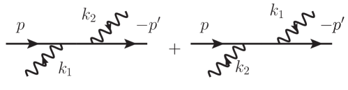
Figure 3: Feynman diagrams for the Compton scattering amplitude in the standard formalism.

8 The fermion self-energy

Since the master formulae given in equations (117, 118) hold off-shell, for the $N=2$ case they can, by sewing together the two photon legs, be used for the construction of the one-loop fermion self energy, indicated in Figure 4. We will carry out this calculation for an arbitrary dimension $D$ and gauge parameter $\xi$, and in close analogy to the worldline calculation of the self-energy in scalar QED performed in 102 .

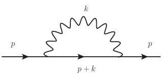
Figure 4: Electron self-energy diagram.

8.1 Construction of the self energy diagram by sewing

The dressed electron propagator in momentum space for $N=2$ is

$$S_{2}^{p^{\prime}p}=\left(\not{p}^{\prime}+m\right)K_{2}^{p^{\prime}p}(k_{1},\varepsilon_{1};k_{2},\varepsilon_{2})-\not{\varepsilon}_{1}K_{1}^{p^{\prime}+k_{1},p}(k_{2},\varepsilon_{2})-\not{\varepsilon}_{2}K_{1}^{p^{\prime}+k_{2},p}(k_{1},\varepsilon_{1})\,.$$ (125)

We can immediately apply the decomposition (LABEL:NdressedmasterpABC) of $K_{2}$ with the explicit results for the coefficients in (LABEL:A2B2C2). Sewing consists of replacing $k_{1}=-k=-k_{2}$ which forces also $p^{\prime}=-p$ and setting

$$\varepsilon_{1\mu}\varepsilon_{2\nu}\rightarrow\frac{\delta_{\mu\nu}}{k^{2}}-(1-\xi)\frac{k_{\mu}k_{\nu}}{k^{4}}\,,$$ (126)

which generates the photon propagator in an arbitrary covariant gauge. Following these substitutions, we then integrate over the loop momentum $k^{\mu}$.

With these identifications it is easy to check that $C_{2}\big{|}_{-k_{1}=k=k_{2}}=0$ and that

$$B_{2}^{\alpha\beta}\big{|}_{-k_{1}=k=k_{2}}\propto Dk^{\alpha}k^{\beta}+k^{2}\delta^{\alpha\beta}+2(1-\xi)k^{\alpha}k^{\beta}\,.$$ (127)

Multiplying this into the anti-symmetric matrix $\sigma^{\alpha\beta}$ gives a result that vanishes. This leaves $A_{2}$ that is split into its scalar and spin parts that take the following form after sewing:

$$A_{2}^{\textrm{scal}}\big{|}_{-k_{1}=k=k_{2}} \rightarrow\frac{2}{k^{2}}\left[D-\frac{\left(2p+k\right)^{2}}{(p+k)^{2}+m^{2}}-\left(1-\xi\right)\left(1-\frac{k\cdot(2p+k)\,\,(2p+k)\cdot k}{k^{2}\left((p+k)^{2}+m^{2}\right)}\right)\right]\,,$$

$$A_{2}^{\textrm{spin}}\big{|}_{-k_{1}=k=k_{2}} \rightarrow-\frac{2(D-1)}{(p+k)^{2}+m^{2}}\,,$$ (128)

where we have taken advantage of the freedom to change the variable of integration $k\rightarrow-k$ to simplify the results. Note that the spin contribution to $A$ is independent of the gauge parameter since the spin interaction is already written in terms of the field strength tensor, whilst the gauge dependent scalar piece is familiar from scalar QED – see 102 . Putting these together the contribution to the self energy from $A_{2}$ becomes ($d^{D}\bar{k}:=\frac{d^{D}k}{(2\pi)^{D}}$)

$$A_{2}^{\textrm{sew}}=\int\frac{d^{D}\bar{k}}{k^{2}}\left[D-\frac{(2p+k)^{2}+(D-1)k^{2}}{(p+k)^{2}+m^{2}}+(1-\xi)\left(\frac{(k^{2}+2p\cdot k)^{2}}{k^{2}\left((p+k)^{2}+m^{2}\right)}-1\right)\right].$$ (129)

(we have dropped a factor of $2$ that is over- counted due to the permutation symmetry of external legs before the sewing takes place). Now, the very first and very last terms correspond to the diagrams with the seagull vertex and these vanish in dimensional regularisation. They can therefore be dropped so that (reinstating the electron charge)

$$K^{p^{\prime}p}_{(2,{\rm sew})} = e^{2}\int\frac{d^{D}\bar{k}}{k^{2}}\left[\frac{(2p+k)^{2}+(D-1)k^{2}}{(m^{2}+p^{2})^{2}[m^{2}+(p+k)^{2}]}-(1-\xi)\frac{(k^{2}+2p\cdot k)^{2}}{k^{2}(m^{2}+p^{2})^{2}[m^{2}+(p+k)^{2}]}\right].$$ (130)

We must add to this the subleading terms. Likewise using the $N=1$ result, (94), applying the sewing procedure to $-\not{\varepsilon}_{1}K_{1}$ and $-\not{\varepsilon}_{2}K_{1}$ we find that each such term provides (here $j\neq i$)

$$-\varepsilon\!\!\!\raise 0.6458pt\hbox{/}_{i}K_{(1,\textrm{sew})}^{p^{\prime}+k_{i},p}(k_{j},\varepsilon_{j})=\int\frac{d^{D}\bar{k}}{k^{2}}\left[\frac{(2\not{p}-(D-2)\not{k})}{(p^{2}+m^{2})((p+k)^{2}+m^{2})}-(1-\xi)\frac{\not{k}}{k^{2}}\frac{k^{2}+2p\cdot k}{(p^{2}+m^{2})((p+k)^{2}+m^{2})}\right].$$ (131)

After combining these terms with (130) and using partial fraction decomposition, only five different integrals remain to be computed, and those are already known from the scalar QED case 102 :

$$I_{1} =\int\frac{d^{D}q}{(2\pi)^{D}}\,\frac{1}{[m^{2}+(p+q)^{2}]}\,\,=\frac{(m^{2})^{\frac{D}{2}-1}}{(4\pi)^{\frac{D}{2}}}\Gamma\Big{(}1-\frac{D}{2}\Big{)}\,;$$

$$I_{2} =\int\frac{d^{D}q}{(2\pi)^{D}}\frac{1}{q^{2}[m^{2}+(p+q)^{2}]}=-\frac{(m^{2})^{\frac{D}{2}-2}}{(4\pi)^{\frac{D}{2}}}\Gamma\Big{(}1-\frac{D}{2}\Big{)}\,_{2}F_{1}\Big{(}2-\frac{D}{2},1;\frac{D}{2};-\frac{p^{2}}{m^{2}}\Big{)}\,;$$

$$I_{3}^{\mu} =\int\frac{d^{D}q}{(2\pi)^{D}}\frac{q^{\mu}}{q^{2}[m^{2}+(p+q)^{2}]}=-\frac{p^{\mu}}{2p^{2}}\left[I_{1}+(p^{2}+m^{2})I_{2}\right]\,;$$

$$J_{1} =\int\frac{d^{D}q}{(2\pi)^{D}}\frac{1}{q^{4}[m^{2}+(p+q)^{2}]}=\frac{(m^{2})^{\frac{D}{2}-3}}{(4\pi)^{\frac{D}{2}}}\Gamma\Big{(}1-\frac{D}{2}\Big{)}\,_{2}F_{1}\Big{(}3-\frac{D}{2},2;\frac{D}{2};-\frac{p^{2}}{m^{2}}\Big{)}\,;$$

$$J_{2}^{\mu} =\int\frac{d^{D}q}{(2\pi)^{D}}\frac{q^{\mu}}{q^{4}[m^{2}+(p+q)^{2}]}=-\frac{p^{\mu}}{2p^{2}}\left[I_{2}+(p^{2}+m^{2})J_{1}\right]\,.$$

In terms of these integrals, we can write the two contributions to $S_{(2,{\rm sew})}^{p^{\prime}p}$ as

$$({\not{p}}^{\prime}+m)K^{p^{\prime}p}_{(2,{\rm sew})} =e^{2}\frac{{\not{p}}^{\prime}+m}{(m^{2}+p^{2})^{2}}\Big{[}4p^{2}I_{2}+4p\cdot I_{3}+DI_{1}+(m^{2}+p^{2})^{2}(\xi-1)J_{1}\Big{]}$$ (133)

and

$$-\not{\varepsilon}_{(i,\rm sew)}K^{p^{\prime}+k_{j},p}_{(1,\rm sew)}=\frac{e^{2}}{m^{2}+p^{2}}\Big{[}2\not{p}I_{2}-(D-2)\not{I}_{3}-(\xi-1)(m^{2}+p^{2})\not{J}_{2}\Big{]}.$$ (134)

Using the integration results above, we may write the contribution to the self energy in the following way:

$$S^{p^{\prime}p}_{(2,{\rm sew})} =e^{2}\frac{({\not{p}}^{\prime}+m)}{(m^{2}+p^{2})^{2}}\frac{(m^{2})^{\frac{D}{2}-2}}{(4\pi)^{\frac{D}{2}}}\Gamma\Big{(}1-\frac{D}{2}\Big{)}\Bigg{\{}(D-2)m^{2}+2(m^{2}-p^{2})\,_{2}F_{1}\Big{(}2-\frac{D}{2},1;\frac{D}{2};-\frac{p^{2}}{m^{2}}\Big{)}$$

$$\hskip 142.26378pt+(\xi-1)\frac{(m^{2}+p^{2})^{2}}{m^{2}}\,_{2}F_{1}\Big{(}3-\frac{D}{2},2;\frac{D}{2};-\frac{p^{2}}{m^{2}}\Big{)}\Bigg{\}}$$

$$-e^{2}\frac{{\not{p}}^{\prime}}{2p^{2}(m^{2}+p^{2})}\frac{(m^{2})^{\frac{D}{2}-2}}{(4\pi)^{\frac{D}{2}}}\Gamma\Big{(}1-\frac{D}{2}\Big{)}\Bigg{\{}-\left[4p^{2}+(D-2)(m^{2}+p^{2})\right]\,_{2}F_{1}\Big{(}2-\frac{D}{2},1;\frac{D}{2};-\frac{p^{2}}{m^{2}}\Big{)}+(D-2)m^{2}$$

$$-(\xi-1)(m^{2}+p^{2})\left[\,{}_{2}F_{1}\Big{(}2-\frac{D}{2},1;\frac{D}{2};-\frac{p^{2}}{m^{2}}\Big{)}-\frac{m^{2}+p^{2}}{m^{2}}\,_{2}F_{1}\Big{(}3-\frac{D}{2},2;\frac{D}{2};-\frac{p^{2}}{m^{2}}\Big{)}\right]\Bigg{\}}.$$ (135)

We are not quite done, however, as we should amputate the external fermions according to (119)

$$\hskip 3.00003pt\widehat{S}\hskip 3.99994pt\,^{p^{\prime}p}_{(2,\rm sew)}=(-\not{p}^{\prime}+m)\,S^{p^{\prime}p}_{(2,\rm sew)}\,(\not{p}+m)\,;$$ (136)

doing this we can decompose the final result to (our notation follows Dav )

$$\hskip 3.00003pt\widehat{S}\hskip 3.99994pt\,^{p^{\prime}p}_{2,\rm sew}=\alpha(p^{2},D){\not{p}}^{\prime}+\beta(p^{2},D)1\!\!1\,\\$$

where

$$\alpha(p^{2},D) =\frac{e^{2}}{2p^{2}}\frac{(m^{2})^{\frac{D}{2}-2}}{(4\pi)^{\frac{D}{2}}}\Gamma\Big{(}1-\frac{D}{2}\Big{)}(D-2)\bigg{\{}\,_{2}F_{1}\Big{(}2-\frac{D}{2},1;\frac{D}{2};-\frac{p^{2}}{m^{2}}\Big{)}\,(m^{2}-p^{2})\Big{[}1+\frac{\xi-1}{D-2}\Big{]}-m^{2}$$

$$\hskip 142.26378pt-\,_{2}F_{1}\Big{(}3-\frac{D}{2},2;\frac{D}{2};-\frac{p^{2}}{m^{2}}\Big{)}\frac{(m^{2}+p^{2})^{2}}{m^{2}}\frac{\xi-1}{D-2}\bigg{\}}\,,$$

$$\beta(p^{2},D) =\frac{e^{2}(m^{2})^{\frac{D}{2}-2}\,m}{(4\pi)^{\frac{D}{2}}}\Gamma\Big{(}1-\frac{D}{2}\Big{)}(D+\xi-1)\,_{2}F_{1}\Big{(}2-\frac{D}{2},1;\frac{D}{2};-\frac{p^{2}}{m^{2}}\Big{)}\,.$$

Further simplification can be achieved by using the following identity for the hypergeometric function ${}_{2}F_{1}$ which we prove in appendix D:

$${}_{2}F_{1}(a,1,2-a;-z)(1-z)(1-2a)+{}_{2}F_{1}(a+1,2,2-a;-z)(1+z)^{2}=2(1-a)\,,$$ (138)

so that with $a=2-\frac{D}{2}$ and $z=\frac{p^{2}}{m^{2}}$ we get

$${}_{2}F_{1}\Big{(}2-\frac{D}{2},1,\frac{D}{2};-\frac{p^{2}}{m^{2}}\Big{)}(m^{2}-p^{2})(D-3)+{}_{2}F_{1}\Big{(}3-\frac{D}{2},2,\frac{D}{2};-\frac{p^{2}}{m^{2}}\Big{)}\frac{(m^{2}+p^{2})^{2}}{m^{2}}=(D-2)m^{2}.$$ (139)

Applying this identity to the coefficient function $\alpha(p^{2},D)$ we obtain the simpler representation

$$\alpha(p^{2},D)=\frac{e^{2}}{2p^{2}}\frac{(D-2)(m^{2})^{\frac{D}{2}-2}}{(4\pi)^{\frac{D}{2}}}\Gamma\Big{(}1-\frac{D}{2}\Big{)}\xi\bigg{\{}(m^{2}-p^{2})\,_{2}F_{1}\Big{(}2-\frac{D}{2},1;\frac{D}{2};-\frac{p^{2}}{m^{2}}\Big{)}-m^{2}\bigg{\}}\,.$$

(141)

In particular, it can now be seen that the coefficient function $\alpha(p^{2},D)$ is absent for $\xi=0$ (Landau gauge).

Davydychev et al. have computed the self-energy in an arbitrary gauge and dimension for a non-Abelian $SU(N)$ theory Dav . We find complete agreement with their results after putting their group parameter $C_{F}=1$ for the $U(1)$ symmetry of QED and transforming to Euclidean space (note that their gauge parameter, $\xi_{D}$, is related to ours by $\xi_{D}=1-\xi$).

8.2 Special gauge choices

Given that our treatment of the propagator naturally splits it up into the two terms that we have referred to as leading and subleading, we pause here to discuss a natural question that arises with respect to the gauge parameter, $\xi$, that we have so far left arbitrary. We will show that it is possible to choose $\xi$ such that either one of these pieces vanishes.

Firstly we consider removing the subleading piece. This cannot be done at the level of the integrand in (131) so we instead consider the final two terms in (135). Applying (139), one is led to the following value of $\xi$ that makes these two terms cancel, which we call $\xi_{1}(p^{2},D)$:

$$\xi_{1}(p^{2},D)=1+\frac{[4p^{2}+(D-2)(p^{2}+m^{2})]{}_{2}F_{1}(2-\frac{D}{2},1;\frac{D}{2};-\frac{p^{2}}{m^{2}})-(D-2)m^{2}}{(D-2)m^{2}-{}_{2}F_{1}(2-\frac{D}{2},1;\frac{D}{2};-\frac{p^{2}}{m^{2}})[m^{2}+p^{2}+(D-3)(m^{2}-p^{2})]}.$$

(142)

However, this gauge parameter cannot be used in $D=4$, since the denominator becomes singular. In fact, in four dimensions the $\frac{1}{\epsilon}$ - pole of the subleading term is gauge independent, and proportional to the expression

$$\frac{e^{2}}{m^{2}+p^{2}}\left[(p^{2}-m^{2})\not{p}+2mp^{2}\right]\,.$$ (143)

The gauge parameter can, however, be used for QED in $D=2$ dimensions, where it becomes

$$\xi_{1}(p^{2},D)=-1-2(D-2)+\ldots$$ (144)

Here we give also the linear term in the $\epsilon$ expansion since, due to the pole contained in the prefactor $\Gamma(1-\frac{D}{2})$ in (135), it will have to be included if one wishes to remove the subleading term completely.

For the leading contribution, the analysis is the same. We find that it vanishes for a gauge parameter $\xi_{2}(p^{2},D)$,

$$\xi_{2}(p^{2},D)=1+\frac{(D-2)m^{2}+2(m^{2}-p^{2}){}_{2}F_{1}(2-\frac{D}{2},1;\frac{D}{2};-\frac{p^{2}}{m^{2}})}{(D-3)(m^{2}-p^{2}){}_{2}F_{1}(2-\frac{D}{2},1;\frac{D}{2};-\frac{p^{2}}{m^{2}})-(D-2)m^{2}}\,.$$ (145)

This time the gauge parameter does not become singular in four dimensions, and expanding around $D=4$ we find that the leading contribution to the propagator can be removed using

$$\xi_{2}(p^{2},D)=3\frac{p^{2}-m^{2}}{m^{2}+p^{2}}+\frac{p^{2}-m^{2}}{m^{2}+p^{2}}\left[3\frac{m^{2}}{p^{2}}\log\left(1+\frac{p^{2}}{m^{2}}\right)-2\right](D-4)+\ldots$$ (146)

Note that, in the massless limit, this becomes $\xi_{2}(p^{2},D)\rightarrow 3-2(D-4)$, whose constant term corresponds to Yennie-Fried gauge, $\xi=3$. On the other hand, expanding around $D=2$ we find

$$\xi_{2}(p^{2},D)=-1+\frac{3p^{2}-m^{2}}{m^{2}-p^{2}}(D-2)+\ldots$$ (147)

Thus in $D=2$ both gauge parameters start with $\xi=-1$, so that here we can achieve more than in four dimensions: we can remove the pole of the leading and subleading contribution simultaneously, and the finite part of one or the other. This does not come unexpected, since it had been noted already in 94 that the $\xi=-1$ gauge in two dimensions has the property of removing the divergence of the one-loop fermion propagator (which in two dimensions is an IR one). More recently, this property has turned out to be extremely useful for multiloop calculations in the Schwinger model 121 . It will be interesting to see whether further simplification can be achieved by one of the generalisations (144), (147).

Another open question is whether there exist similar choices of gauge that can remove various contributions at higher order, since it would be advantageous to have the option of removing the leading term, especially when considering amplitudes with a large number of photons attached to the line. This is because the leading contribution at order $N$, $({\not{p}}^{\prime}+m)K_{N}$ involves the $N$-photon kernel which is progressively more complicated than the $N$ subleading contributions of the form $\not{\varepsilon}_{i}K_{N-1}$. This is clear even in the results for $N=1$ or $N=2$ presented above in section 7. At higher order the simplifications gained by being able to discount $K_{N}$ could be substantial and may help to streamline various calculations. We leave this for examination in future work.

9 Conclusions and Outlook

In this article we have presented a new – and long overdue – approach to the worldline path integral representation of the open Dirac-fermion line dressed with $N$ photons. The formalism is designed to extend to the open-line case the main calculational advantages of the well-established worldline formulation of the closed fermion loop, such as:

1. Making possible the derivation of compact master formulas representing whole classes of Feynman diagrams differing by the ordering of the photon legs along a loop or line.

2. Keeping a close analogy between scalar and spinor QED calculations, in particular with respect to the simple dependence on the loop mass.

3. Minimising the effort in Dirac algebra manipulations through the use of the symbol map, which effectively avoids long products of Dirac matrices by an early projection onto the Clifford basis.

4. Allowing the generation of gauge-invariant structures by integration-by-part algorithms, rather than the usual tedious analysis of the QED Ward identities.

Our formalism is based on the second-order approach to spinor QED, which has been known for decades as an alternative to the standard Dirac approach hostler ; morgan but rarely been considered as an alternative for state-of-the-art calculations (although in recent years it has been used as a starting point for the construction of non-standard abelian gauge theories Napsuciale_1 ; Napsuciale_2 ; Mauro ; Mariana_1 ; Mariana_2 ; JEspin ). It is also close in spirit to first-quantised string theory, and thus shares some of the superior organisation of string amplitudes, particularly with respect to gauge invariance, permutation symmetry and worldline supersymmetry.

In the present first part of this series of papers we have focused on the construction of a Bern-Kosower type master formula for the fermion propagator dressed with $N$ photons, still off-shell and geared towards the construction of multiloop amplitudes. We have given this formula in two versions, once using worldline superfields and once via a spin-orbit decomposition that should contain additional physical information. Both versions are amenable to numerical implementation. We have explicitly worked out the cases $N=0,1,2$, and demonstrated in detail how the equivalence to the standard approach works. The $N=2$ result has further been used for a recalculation of the one-loop fermion self energy for arbitrary dimension and arbitrary gauge parameter $\xi$. Cancellations for special values of $\xi$ have been found that look promising for investigation at higher-loop order.

The forthcoming second part will focus on on-shell amplitudes and cross sections involving open fermion lines, and in the third part we will add an external constant field (partial results of the third part have already been published in 113 ; ahmedwild-19 ).

In an independent publication we will use the formalism for an extension of the generalised $2N$-point Landau-Khalatnikov-Fradkin transformation introduced in 102 for scalar QED, to the spinor QED case. Future additional articles will further be devoted to the application of the formalism to multi-loop $g-2$ calculations, and to the derivation of Ball-Chiu form factors. Generalisations to the non-abelian case and to the inclusion of axial couplings are also under consideration.

Appendix A Conventions

On the side of the worldline formalism, we work throughout in Euclidean space with metric $(+++\,+)$, and use Dirac matrices fulfilling $\{\gamma^{\mu},\gamma^{\nu}\}=-2\delta^{\mu\nu}$. On the field theory side, we Wick rotate to Minkowski space with metric $\eta_{\mu\nu}=\textrm{diag}(-++\,+)$, and use $\{\gamma^{\mu},\gamma^{\nu}\}=-2\eta^{\mu\nu}$. We further define $\varepsilon^{0123}=+1$ and $\gamma_{5}=i\gamma^{0}\gamma^{1}\gamma^{2}\gamma^{3}$. The fermion propagator becomes $-i/(\not{p}+m)$ and the first-order Dirac vertex $-ie\gamma^{\mu}$. The sign of the effective action corresponds to a tree-level term $-\frac{1}{4}F_{\mu\nu}F^{\mu\nu}$ in both Euclidean and Minkowskian spacetimes. The covariant derivative is $D_{\mu}=\partial_{\mu}+ieA_{\mu}$. These Minkowski space conventions coincide with the textbook of Srednicki srednicki-book except for the sign of the electric charge and that we use ingoing momenta in Feynman diagrams instead of outgoing ones. The Feynman rules for the second-order formalism have been given in the introduction, Figure 1.

Appendix B Intrinsic worldline approach to the electron propagator

In this appendix, we rederive the path-integral representation of the electron propagator in a more “principled” way, using the principles of quantum mechanics, gauge theory and (worldline) supersymmetry but no field-theory input.

As is well-known, a spin 1/2 particle can be described in a manifestly covariant way by a gauge model with one local supersymmetry on the worldline. For the massless case, the phase space action depends on the particle space time coordinates $x^{\mu}$ joined by the real Grassmann variables $\psi^{\mu}$, supersymmetric partners of the former that supply the degrees of freedom associated to spin. In addition, there are Lagrange multipliers $e$ (the einbein) and $\chi$ (the gravitino), with commuting and anti-commuting character, respectively, that gauge suitable first class constraints (they form the supergravity multiplet in one dimension). Eventually, their effect is to eliminate negative norm states from the physical spectrum, and make the particle model consistent with unitarity at the quantum level.

The action for the massless particle takes the form (given here in Minkowski space)

$$S = \int d\tau\left(p_{\mu}\dot{x}^{\mu}+\frac{i}{2}\psi_{\mu}\dot{\psi}^{\mu}-eH-i\chi Q\right)\,,$$ (148)

where the first class constraints are given by

$$H=\frac{1}{2}p^{2}\;,\qquad Q=p_{\mu}\psi^{\mu}\,,$$ (149)

that generate through Poisson brackets the $N=1$ susy algebra in one dimension

$$\{Q,Q\}=-2iH\;.$$ (150)

This algebra is computed by using the graded Poisson brackets of the phase space coordinates, $\{x^{\mu},p_{\nu}\}=\delta^{\mu}_{\nu}$ and $\{\psi^{\mu},\psi_{\nu}\}=-i\delta^{\mu}_{\nu}$, fixed by the symplectic term of the action.

The gauge transformations are generated on the phase space coordinates $(x,p,\psi)$ through Poisson brackets with $V\equiv\zeta H+i\epsilon Q$, where $\zeta$ and $\epsilon$ are local parameters with appropriate Grassmann parity whilst on gauge fields the gauge transformations are obtained by using the structure constants of the constraint algebra and turn out to be

$$\delta x^{\mu}=\zeta p^{\mu}+i\epsilon\psi^{\mu} \,;\qquad\delta p_{\mu}=0\,;\qquad\delta\psi^{\mu}=-\epsilon p^{\mu}\,;$$ (151)

$$\delta e =\dot{\zeta}+2i\chi\epsilon\,;\quad\delta\chi=\dot{\epsilon}\ .$$ (152)

Let us now study canonical quantisation to uncover the consequences of the constraints, and see how the Dirac equation emerges. Promoting the phase space variables to operators one finds the following (anti) commutation relations

$$[\hat{x}^{\mu},\hat{p}_{\nu}]=i\delta^{\mu}_{\nu}\ ,\quad\quad\{\hat{\psi}^{\mu},\hat{\psi}^{\nu}\}=\eta^{\mu\nu},$$ (153)

while other graded commutators vanish. The former relations are realised on the usual infinite dimensional Hilbert space of functions of the particle coordinates. The latter relations are seen to give rise to a Clifford algebra that may be identified with the algebra of the Dirac gamma matrices $\Gamma^{\mu}$, satisfying $\{\Gamma^{\mu},\Gamma^{\nu}\}=2\eta^{\mu\nu}$ and as such they can be realised on the finite dimensional Hilbert space of spinors as

$$\hat{\psi}^{\mu}\ \to\ \frac{1}{\sqrt{2}}\,\Gamma^{\mu}\,,$$ (154)

with dimension $2^{\left[\frac{D}{2}\right]}$. The full Hilbert space is the direct product of the two Hilbert spaces obtained above and is identified with the space of spinor fields.

The full information of the physical states, $\left|\Psi\right>$, resides in the constraints implemented à la Dirac. In particular, the constraint due to the susy charge $\hat{Q}=\hat{p}_{\mu}\hat{\psi}^{\mu}$ gives rise to the massless Dirac equations

$$\hat{p}_{\mu}\hat{\psi}^{\mu}|\Psi\rangle=0\quad\to\quad\Gamma^{\mu}\partial_{\mu}\Psi(x)=0.$$ (155)

Likewise the constraint $\hat{H}|\Psi\rangle=0$ leads to the massless Klein Gordon equation for all components of the spinor $\Psi$, and is automatically satisfied as a consequence of the algebra $\hat{Q}^{2}=\hat{H}$. Thus, we recognise how a first quantised description of a spin 1/2 particle emerges from canonical quantisation of a constrained system.

To study the corresponding path integral quantisation it is useful to eliminate the momenta $p_{\mu}$ to obtain the action in configuration space

$$S_{c}[x,\psi,e,\chi]=\int d\tau\left(\frac{1}{2}e^{-1}(\dot{x}^{\mu}-i\chi\psi^{\mu})^{2}+\frac{i}{2}\psi_{\mu}\dot{\psi}^{\mu}\right)\,,$$ (156)

whose local symmetries may be recovered from the phase space ones.

Finally, a Wick rotation to Euclidean proper time produces the Euclidean action

$$S_{E}[x,\psi,e,\chi]=\int d\tau\left(\frac{1}{2}e^{-1}(\dot{x}^{\mu}-\chi\psi^{\mu})^{2}+\frac{1}{2}\psi_{\mu}\dot{\psi}^{\mu}\right).$$ (157)

The massive case is slightly more subtle. To obtain it we use a method of introducing a mass term starting from the massless theory formulated in one dimension higher. We denote the extra dimension by $x^{5}$, and coordinates by $x^{M}=(x^{\mu},x^{5})$, so that indices split as $M=(\mu,5)$. The massless spin 1/2 particle in one dimension higher is described by the phase space action

$$S=\int d\tau\left(p_{M}\dot{x}^{M}+\frac{i}{2}\psi_{M}\dot{\psi}^{M}-\frac{e}{2}p_{M}p^{M}-i\chi\,p_{M}\psi^{M}\right).$$ (158)

Now one imposes the constraint $p_{5}=m$, where $m$ is a constant to be identified as the mass of the particle in one dimension lower. The action now takes the form

$$S=\int d\tau\left(p_{\mu}\dot{x}^{\mu}+m\dot{x}^{5}+\frac{i}{2}\psi_{\mu}\dot{\psi}^{\mu}+\frac{i}{2}\psi^{5}\dot{\psi}^{5}-e\frac{1}{2}(p_{\mu}p^{\mu}+m^{2})-i\chi(p_{\mu}\psi^{\mu}+m\psi^{5})\right).$$ (159)

The term with the coordinate $x^{5}$ is a total derivative and can be dropped from the action but $\psi^{5}$ is retained. Let us check that this indeed describes a free, massive spin 1/2 particle, at least in even dimensions. We focus directly on $D=4$ dimensions and note that on top of the operators in (153) one finds the extra fermionic operator $\hat{\psi}^{5}$ that can be identified with $\Gamma^{5}/\sqrt{2}$, where $\Gamma_{5}$ is the usual chirality matrix obeying $(\Gamma_{5})^{2}=1$. The susy constraint $p_{\mu}\psi^{\mu}+m\psi^{5}=0$ becomes at the quantum level

$$(-i\Gamma^{\mu}\partial_{\mu}+m\Gamma^{5})\Psi=0\;.$$ (160)

One can multiply this by $\Gamma^{5}$ and recognise that the set $\tilde{\gamma}^{\mu}=\Gamma^{5}\Gamma^{\mu}$ satisfies the standard (with signature $-+++$) Clifford algebra $\{\tilde{\gamma}^{\mu},\tilde{\gamma}^{\nu}\}=-2\eta^{\mu\nu}$ which leads to the massive Dirac equation

$$(-i\not{\partial}+m)\Psi=(\not{p}+m)\Psi=0\,,$$ (161)

as required.

However, our goal here is to get the massive Dirac equation through path-integral quantisation. Let us start from the action in eq. (158), suitably Wick rotated to

$$S[x,p,\psi,\psi_{5},e,\chi]=\int d\tau\Bigl{[}-ip_{\mu}\dot{x}^{\mu}+\frac{1}{2}\psi_{\mu}\dot{\psi}^{\mu}+\frac{1}{2}\psi^{5}\dot{\psi}^{5}+\frac{e}{2}(p_{\mu}p^{\mu}+m^{2})+i\chi(p_{\mu}\psi^{\mu}+m\psi^{5})\Bigr{]}\,.$$ (162)

It enters the path integral as

$$Z\sim\int\frac{{D}x{D}p{D}\psi{D}\psi_{5}{D}e{D}\chi}{\rm Vol(Gauge)}\ \,{\rm e}^{-S[x,p,\psi,\psi_{5},e,\chi]}\;.$$ (163)

Integrating out the momentum gives the configuration space action. Before gauge fixing, and in Euclidean time, it takes the form

$$S[x,\psi,\psi_{5},e,\chi]=\int_{0}^{1}d\tau\,\frac{1}{2}\left(e^{-1}(\dot{x}-\chi\psi)^{2}+\psi\dot{\psi}+\psi_{5}\dot{\psi}_{5}+em^{2}+2i\chi m\psi_{5}\right)\,,$$ (164)

where we have suppressed obvious indices. There are two local symmetries to take care of, reparameterisations and local supersymmetry, with gauge fields $e$ and $\chi$, respectively.

We start using the reparameterisation invariance to fix $e(\tau)\equiv 2T$ in that Lagrangian which, on the line, reduces the path integral $\int De(\tau)$ to the proper-time integral with trivial Faddeev-Popov measure $\int_{0}^{\infty}dT$. For fixed $T$, we then rescale $\tau\to T\tau$. The gravitino field $\chi$ is the gauge field for the local worldline supersymmetry, and on an interval can be gauge-fixed to a constant Grassmann variable $\Theta$, the super-partner of the global proper-time $T$. The gravitino path integral $\int D\chi(\tau)$ then gets replaced by the ordinary Grassmann integral $\int d\Theta$.

Next, let us consider the terms in the worldline action that depend on the gravitino field $\chi(\tau)$. Since $\chi^{2}(\tau)=0$, those terms can be written as

$$S_{\chi} \equiv \frac{1}{T}\int_{0}^{T}d\tau\chi\Bigl{(}-{1\over 2}\dot{x}\cdot\psi+im\psi_{5}\Bigr{)}\,.$$ (165)

We can then use the nilpotency of $\Theta$ to replace the exponential by its argument, and perform the integral:

$$\int D\chi\,\,{\rm e}^{-S_{\chi}}=\int d\Theta\,\,{\rm e}^{-S_{\Theta}}=\frac{1}{T}\int_{0}^{T}d\tau\Bigl{(}{1\over 2}\dot{x}\cdot\psi-im\psi_{5}\Bigr{)}\,.$$ (166)

At this stage, we have

$$Z=\int_{0}^{\infty}dT\,\,{\rm e}^{-m^{2}T}\int_{I}{D}x{D}\psi{D}\psi_{5}\frac{1}{T}\int_{0}^{T}d\tau\Bigl{(}{1\over 2}\dot{x}\cdot\psi-im\psi_{5}\Bigr{)}\,\,{\rm e}^{-\int_{0}^{T}d\tau\,\left(\frac{1}{4}\dot{x}^{2}+\frac{1}{2}\psi\dot{\psi}+\frac{1}{2}\psi_{5}\dot{\psi}_{5}\right)}\,.$$

(167)

We must now think about the boundary conditions to be imposed on the Grassmann fields $\psi(\tau)$ and $\psi_{5}(\tau)$. For the coordinate path integral, passing from the closed loop to the open line case means replacing the homogeneous boundary conditions $x^{\mu}(T)-x^{\mu}(0)=0$ by inhomogeneous ones,

$$x^{\mu}(T)-x^{\mu}(0)=x^{\prime\mu}-x^{\mu}\,,$$ (168)

so that we calculate off-diagonal elements of the kernel. Likewise the propagator will depend upon the initial and final spin states, so we should expect that the anti-periodicity condition

$$\psi^{\mu}(T)+\psi^{\mu}(0)=0\,,$$ (169)

be replaced by the inhomogeneous (“twisted”) condition

$$\psi^{\mu}(T)+\psi^{\mu}(0)=\eta^{\mu}\,,$$ (170)

where $\eta^{\mu}$ is a constant external Grassmann vector that should generate the spin structure of the kernel. But here we run into the following subtlety with the variation of the action. The variation of the free particle action is

$$\delta S_{\psi} =\int_{0}^{T}d\tau\,\delta\psi_{\mu}\dot{\psi}^{\mu}+{1\over 2}\bigl{(}\psi_{\mu}\delta\psi^{\mu}\bigr{)}\Big{|}^{\tau=T}_{\tau=0}.$$ (171)

The first term gives us the local equation of motion $\dot{\psi}^{\mu}=0$. In the closed loop case, we would have anti-periodic boundary conditions on $\psi$ and $\delta\psi$ which would lead to the vanishing of the surface term in (171). In the open-line case, instead we have (170) but $\delta\psi$ remains anti-periodic, resulting in a non-zero contribution from the surface term,

$${1\over 2}\bigl{(}\psi\cdot\delta\psi\bigr{)}\Big{|}^{\tau=T}_{\tau=0}={1\over 2}\eta\cdot\delta\psi(T)\,.$$ (172)

If the choice of twisted boundary conditions is to be consistent, this non-local term should be cancelled by something. To see what is missing, note that we can switch from anti-periodic boundary conditions on $\psi(\tau)$ to twisted ones on $\xi(\tau)$ by setting

$$\psi^{\mu}(\tau)+{1\over 2}\eta^{\mu}=\xi^{\mu}(\tau)$$ (173)

and that the result of this transformation can be written as

$$\int_{0}^{T}d\tau\,{1\over 2}\psi(\tau)\cdot\dot{\psi}(\tau)\longrightarrow\int_{0}^{T}d\tau\,{1\over 2}\xi(\tau)\cdot\dot{\xi}(\tau)+{1\over 2}\xi(T)\cdot\xi(0)\,.$$ (174)

Under an infinitesimal shift of $\xi(\tau)$, the second term on the right-hand side produces an additional term ${1\over 2}\delta\xi(T)\cdot\xi(0)+{1\over 2}\xi(T)\cdot\delta\xi(0)$ which is just right to cancel the surface term in (171) (with $\psi$ now replaced by $\xi$). This leads us to understand that the precise version of (167) is

$$Z =\int_{0}^{\infty}dT\,\,{\rm e}^{-m^{2}T}\int_{x(0)=x^{\prime}}^{x(T)=x}{D}x\int_{\xi(T)+\xi(0)=\eta}{D}\xi\hskip 30.0pt\int_{\xi_{5}(T)+\xi_{5}(0)=\eta_{5}}{D}\xi_{5}\hskip 40.0pt\frac{1}{T}\int_{0}^{T}d\tau\Bigl{(}{1\over 2}\dot{x}\cdot\xi-im\xi_{5}\Bigr{)}$$

$$\times\,\,{\rm e}^{-\int_{0}^{T}d\tau\,\frac{1}{4}\dot{x}^{2}}\,\,{\rm e}^{-\int_{0}^{T}d\tau\,\frac{1}{2}\xi\cdot\dot{\xi}-\frac{1}{2}\xi(T)\cdot\xi(0)}\,\,{\rm e}^{-\int_{0}^{T}d\tau\,\frac{1}{2}\xi_{5}\dot{\xi}_{5}-\frac{1}{2}\xi_{5}(T)\xi_{5}(0)}\,.$$ (175)

We now turn our attention to the prefactor $({1\over 2}\dot{x}\cdot\xi-im\xi_{5})$. In the second term, the equation of motion $\dot{\xi}_{5}=0$ means that Ehrenfest’s theorem gives

$${d\over d\tau}\langle\xi_{5}(\tau)\rangle=0\,.$$ (176)

Thus this term is actually independent of $\tau$, so that we are free to replace it by the average of its endpoint values, and then apply the boundary conditions:

$$\langle\xi_{5}(\tau)\rangle\longrightarrow{1\over 2}\bigl{(}\xi_{5}(T)+\xi_{5}(0)\bigr{)}={1\over 2}\eta_{5}\,.$$ (177)

Similarly, for the first term we can invoke the above-mentioned fact that $Q=\dot{x}\cdot\xi$ is the conserved charge associated to the worldline supersymmetry transformations (LABEL:susy). Thus we have also

$${d\over d\tau}\langle\dot{x}\cdot\xi\rangle=0\,,$$ (178)

and we use this again to replace the $\tau$ - integrand by the average of its endpoint values:

$$\langle\dot{x}(\tau)\cdot\xi(\tau)\rangle\longrightarrow{1\over 2}\bigl{(}\dot{x}(T)\cdot\xi(T)+\dot{x}(0)\cdot\xi(0)\bigr{)}$$ (179)

Now we need to Figure out the effect of a factor $\dot{x}^{\mu}(T)$ or $\dot{x}^{\mu}(0)$ inserted into the free $x$ - path integral. An insertion of $\dot{x}(T)$ into the free path integral will, after the transformations (42),(43), turn into

$$\dot{x}(T)\longrightarrow\frac{x^{\prime}-x}{T}+\dot{q}(T)\,.$$ (180)

The fluctuation term $\dot{q}(T)$ leads to an insertion under the path integral over $q$ that is odd in $q$, and thus vanishes. Moreover from the explicit result for the free $x$-space propagator, (LABEL:bk-like-x) with $N=0$, we see that this term could as well be represented as a derivative $-2{\partial\over\partial x^{\prime\mu}}$, acting on the final point of the trajectory. Similarly, an insertion $\dot{x}(0)$ can be represented as a derivative $2{\partial\over\partial x^{\mu}}$ of the amplitude with respect to the initial point $x$ which by translation invariance can be replaced by $-2{\partial\over\partial x^{\prime\mu}}$. After this, we are ready to use the Grassmann boundary conditions to replace further

$$\dot{x}(T)\cdot\xi(T)+\dot{x}(0)\cdot\xi(0)\longrightarrow-2{\partial\over\partial x^{\prime}}\cdot\bigl{(}\xi(T)+\xi(0)\bigr{)}\longrightarrow-2{\partial\over\partial x^{\prime}}\cdot\eta\,.$$ (181)

The prefactor term is now completely expressed in terms of external quantities, and does not involve the path integral variables any more. Thus the path integrals can now be performed. The Grassmann path integrals just yield global normalisation factors, independent even of $\eta$ and $\eta_{5}$ (as can be seen most simply by applying the transformation of variables (173) in reverse). The $x$ path integral together with the global $T$ integration yields the free scalar propagator $D^{xx^{\prime}}_{0}$. Thus we have now simply (up to normalisation)

$$Z=\bigl{(}-i\eta\cdot{\partial\over\partial x}+m\eta_{5}\bigr{)}D^{xx^{\prime}}_{0}$$ (182)

The remaining task of matching this to (37) (for the free case $A=0$) parallels our discussion for the operator formalism above. We require a rule for mapping the Grassmann variables to gamma matrices. It would be inconsistent to map $\eta_{5}$ to $1$ and $\eta^{\mu}$ to $-\gamma^{\mu}$, so we are instead led to identify $\eta_{5}$ with $\gamma_{5}$, and reuse the fact that $\gamma_{5}\gamma^{\mu}$ are equivalent to $\gamma^{\mu}$ so we finally choose the assignation

$$\eta_{5}\longrightarrow\gamma_{5},\quad\eta^{\mu}\longrightarrow-\gamma_{5}\gamma^{\mu}\,.$$ (183)

In this way $Z$ gets mapped into $\gamma_{5}S^{xx^{\prime}}$, rather than $S^{xx^{\prime}}$, but this is equivalent, and the best we can do. It may appear awkward to introduce $\gamma_{5}$ in this seemingly non-chiral context, but the fact is that its appearance is a common feature of first-principle approaches to the path integral representation of the massive fermion propagator.

Appendix C Path-ordered path integrals and symbol map

In this appendix, we prove the identity (70) that allows us to replace the Feynman spin factor (5) with a path integral over Grassmann variables via the symbol map. Our proof essentially follows fragit .

First, by standard functional calculus we can rewrite

$$\mathcal{P}\left\{e^{-\frac{i}{2}e\int_{0}^{T}d\tau\,\gamma^{\mu}F_{\mu\nu}\gamma^{\nu}}\right\}=\,{\rm e}^{i\frac{e}{2}\int_{0}^{T}d\tau F_{\mu\nu}(x(\tau))\frac{\delta}{\delta\theta_{\nu}(\tau)}\frac{\delta}{\delta\theta_{\mu}(\tau)}}\mathcal{P}\Bigl{[}\,{\rm e}^{\int_{0}^{T}d\tau\,\theta_{\lambda}(\tau)\gamma^{\lambda}}\Bigr{]}\Big{|}_{\theta=0}\,$$ (184)

(185)

with Grassmann-valued functions $\theta^{\mu}(\tau)$ that anticommute with the $\gamma^{\mu}$.

Next, we remove the path-ordering operator using the identity

$$\mathcal{P}\Bigl{[}\,{\rm e}^{\int_{0}^{T}d\tau\,\theta(\tau)\cdot\gamma}\Bigr{]}=\,{\rm e}^{\int_{0}^{T}d\tau\,\theta(\tau)\cdot\gamma}\,{\rm e}^{\frac{1}{2}\int_{0}^{T}d\tau\,\int_{0}^{T}d\tau^{\prime}\theta^{\mu}(\tau){\rm sign}(\tau-\tau^{\prime})\delta_{\mu\nu}\theta^{\nu}(\tau^{\prime})}\,.$$ (186)

Now on the right-hand side the first exponential can be rewritten as

$$\,{\rm e}^{\int_{0}^{T}d\tau\,\theta(\tau)\cdot\gamma}=\,{\rm e}^{i\frac{\gamma^{\mu}}{\sqrt{2}}\frac{\partial}{\partial\eta^{\mu}}}\,{\rm e}^{i\sqrt{2}\int_{0}^{T}d\tau\,\theta_{\nu}(\tau)\eta^{\nu}}\Bigl{|}_{\eta=0}\,,$$ (187)

where the $\eta^{\mu},\mu=1,\ldots,D$ are Grassmann numbers that again must anticommute with the $\gamma^{\mu}$, while the second exponential can be replaced by a Gaussian Grassmann path integral:

$$\,{\rm e}^{\frac{1}{2}\int_{0}^{T}d\tau\int_{0}^{T}d\tau^{\prime}\theta^{\mu}(\tau){\rm sign}(\tau-\tau^{\prime})\delta_{\mu\nu}\theta^{\nu}(\tau^{\prime})}=\frac{\int_{\psi(0)+\psi(T)=0}{D}\psi\,\,{\rm e}^{-\int_{0}^{T}d\tau\left[\frac{1}{2}\psi\cdot\dot{\psi}-i\sqrt{2}\,\theta\cdot\psi\right]}}{\int_{\psi(0)+\psi(T)=0}{D}\psi\,\,{\rm e}^{-\int_{0}^{T}d\tau\frac{1}{2}\psi\cdot\dot{\psi}}}\,.$$ (188)

Here the denominator is the free path-integral normalisation, which is equal to $2^{\frac{D}{2}}$ in $D$ (even) dimensions. Thus the previous three equations can be combined to

$$\mathcal{P}\Bigl{[}\,{\rm e}^{\int_{0}^{T}d\tau\,\theta(\tau)\cdot\gamma}\Bigr{]}=2^{-\frac{D}{2}}\,{\rm e}^{i\frac{\gamma^{\mu}}{\sqrt{2}}\frac{\partial}{\partial\eta^{\mu}}}\int_{\psi(0)+\psi(T)=0}{D}\psi\,\,{\rm e}^{-\int_{0}^{T}d\tau\left[\frac{1}{2}\psi\cdot\dot{\psi}-i\sqrt{2}\,\theta_{\mu}(\psi^{\mu}+\eta^{\mu})\right]}\Bigl{|}_{\eta=0}\,.$$ (189)

Now we act on this with the functional operator of (185). This produces

$$\,{\rm e}^{i\frac{e}{2}\int_{0}^{T}d\tau F_{\mu\nu}(x(\tau))\frac{\delta}{\delta\theta_{\nu}(\tau)}\frac{\delta}{\delta\theta_{\mu}(\tau)}}\,\,{\rm e}^{-\int_{0}^{T}d\tau\left[\frac{1}{2}\psi\cdot\dot{\psi}-i\sqrt{2}\,\theta_{\mu}(\psi^{\mu}+\eta^{\mu})\right]}=\,{\rm e}^{-\int_{0}^{T}d\tau\left[\frac{1}{2}\psi\cdot\dot{\psi}-ie(\psi^{\mu}+\eta^{\mu})F_{\mu\nu}(\psi^{\nu}+\eta^{\nu})\right]}\,,$$

and thus by combining the previous two equations with our starting identity (185) we get

$$\mathcal{P}\left\{\,{\rm e}^{-\frac{1}{2}e\int_{0}^{T}d\tau\,\gamma^{\mu}F_{\mu\nu}\gamma^{\nu}}\right\}=2^{-\frac{D}{2}}\,{\rm e}^{i\frac{\gamma^{\mu}}{\sqrt{2}}\frac{\partial}{\partial\eta^{\mu}}}\int{D}\psi\,\,{\rm e}^{-\int_{0}^{T}d\tau\left[\frac{1}{2}\psi\cdot\dot{\psi}-ie(\psi^{\mu}+\eta^{\mu})F_{\mu\nu}(\psi^{\nu}+\eta^{\nu})\right]}\Bigl{|}_{\eta=0}\,.$$

(191)

The final step is to observe that the operation

$$\,{\rm e}^{i\frac{\gamma^{\mu}}{\sqrt{2}}\frac{\partial}{\partial\eta^{\mu}}}f(\eta)\Bigl{|}_{\eta=0}$$ (192)

order by order just corresponds to the replacement of products of $\eta^{\alpha}$s by antisymmetrised products of $\gamma^{\alpha}$, that is, to the inverse of the symbol map defined in (71). This completes the proof of the identity (70).

Appendix D Proof of the hypergeometric identity (139)

In this appendix we show how to reduce the hypergeometric identity (139)

$${}_{2}F_{1}(a,1;2-a;-z)(1-z)(1-2a)+{}_{2}F_{1}(a+1,2;2-a;-z)(1+z)^{2}=2(1-a)$$ (193)

to known identities. The arguments of the hypergeometric functions appearing in this identity are of the special kind which makes it possible to rewrite them in terms of Associated Legendre functions of the first kind $P^{\mu}_{\nu}(z)$ using the identity (eq. 15.4.15 of abrasteg-book )

$${}_{2}F_{1}(a,b;a-b+1;z)=\Gamma(a-b+1)(1-z)^{-b}(-z)^{\frac{1}{2}(b-a)}P^{b-a}_{-b}\Bigl{(}\frac{1+z}{1-z}\Bigr{)}\qquad(-\infty<z<0)\,.$$

(194)

Applying this identity (with $a$ and $b$ interchanged and $z\to-z$) we find

$${}_{2}F_{1}(a,1;2-a;-z) = \Gamma(2-a)(1+z)^{-a}z^{\frac{a-1}{2}}P^{a-1}_{-a}\Bigl{(}\frac{1-z}{1+z}\Bigr{)}\,,$$

$${}_{2}F_{1}(a+1,2;2-a;-z) = \Gamma(2-a)(1+z)^{-a-1}z^{\frac{a-1}{2}}P^{a-1}_{-a-1}\Bigl{(}\frac{1-z}{1+z}\Bigr{)}\,.$$

For the Legendre functions one has the “varying degree identity” (eq. 8.5.3 of abrasteg-book )

$$(\nu-\mu+1)P^{\mu}_{\nu+1}(x)=(2\nu+1)xP^{\mu}_{\nu}(x)-(\nu+\mu)P_{\nu-1}^{\mu}(x)\,.$$ (196)

Using this identity with $\mu=a-1$, $\nu=-a$ and $x=\frac{1-z}{1+z}$ yields

$$2(1-a)P^{a-1}_{1-a}\Bigl{(}\frac{1-z}{1+z}\Bigr{)}=(1-2a)\frac{1-z}{1+z}P^{a-1}_{-a}\Bigl{(}\frac{1-z}{1+z}\Bigr{)}+P_{-a-1}^{a-1}\Bigl{(}\frac{1-z}{1+z}\Bigr{)}\,.$$ (197)

Multiplying both sides by a factor of $\Gamma(2-a)(1+z)^{1-a}z^{\frac{a-1}{2}}$, and combining the result with (LABEL:hypergeotolegendre), leads to (193) provided that

$$\Gamma(2-a)(1+z)^{1-a}z^{\frac{a-1}{2}}P^{a-1}_{1-a}\Bigl{(}\frac{1-z}{1+z}\Bigr{)}\stackrel{{\scriptstyle!}}{{=}}1\,,$$ (198)

which can be verified using the identity (eq. 8.6.16 of abrasteg-book ),

$$P_{\nu}^{-\nu}(x)=\frac{2^{-\nu}(1-x^{2})^{\frac{1}{2}\nu}}{\Gamma(\nu+1)}\,,$$ (199)

now with $\nu=1-a$ (and $x=\frac{1-z}{1+z}$).

References

• (1) R.P. Feynman, Phys. Rev. 80, 440 (1950).
• (2) R.P. Feynman, Phys. Rev. 84, 108 (1951).
• (3) C. Schubert, Phys. Rep. 355, 73 (2001), arXiv:hep-th/0101036.
• (4) J. P. Edwards and C. Schubert, Technical Report to be published in the proceedings of the workshop “Path Integration in Complex Dynamical Systems,” Leiden, 6 Feb - 10 Feb 2017. arXiv:1912.10004 [hep-th].
• (5) I.K. Affleck, O. Alvarez and N.S. Manton, Nucl. Phys. B 197, 509 (1982).
• (6) G. V. Dunne and C. Schubert, Phys. Rev. D 72, 105004 (2005), arXiv:hep-th/0507174.
• (7) G. V. Dunne, Q.-h. Wang, H. Gies and C. Schubert, Phys. Rev. D 73 065028 (2006), arXiv:hep-th/0602176.
• (8) M. J. Strassler, Nucl. Phys. B 385, 145 (1992), arXiv:hep-ph/9205205.
• (9) Z. Bern and D. A. Kosower, Phys. Rev. Lett. 66, 1669 (1991); Nucl. Phys. B 379, 451 (1992)
• (10) A.M. Polyakov, Gauge Fields and Strings, Harwood (1987).
• (11) Z. Bern, TASI Lectures, Boulder TASI 92, 471, arXiv:9304249 [hep-ph].
• (12) Z. Bern and D.C. Dunbar, Nucl. Phys. B 379 (1992) 562.
• (13) M.G. Schmidt and C. Schubert, Phys. Rev. D 53, 2150 (1996), arXiv:hep-th/9410100.
• (14) M.J. Strassler, SLAC-PUB-5978 (1992) (unpublished).
• (15) C. Schubert, Eur. Phys. J. C5, 693 (1998), arXiv:hep-th/9710067.
• (16) N. Ahmadiniaz, C. Schubert and V.M. Villanueva, JHEP 1301, 312 (2013), arXiv:1211.1821 [hep-th].
• (17) M.J. Strassler, The Bern-Kosower Rules and their Relation to Quantum Field Theory, PhD thesis, Stanford University 1993.
• (18) R.P. Feynman and M. Gell-Mann, Phys. Rev. 109 (1958) 193.
• (19) L.C. Hostler, J. Math. Phys. 26 (1985) 1348.
• (20) A. Morgan, Phys. Lett. B 351 (1995) 249, arXiv:hep-ph/9502230.
• (21) J. Espin, Second-Order Fermions, Ph.D. Thesis, Nottingham Univ. 2015, arXiv:1509.05914 [hep-th].
• (22) G. V. Dunne and C. Schubert, JHEP 0208, 053 (2002), arXiv:hep-th/0205004.
• (23) M.G. Schmidt and C. Schubert, Phys. Lett. B 318, 438 (1993), arXiv:hep-th/9309055.
• (24) D. Cangemi, E. D’Hoker and G.V. Dunne, Phys. Rev. D 51, 2513 (1995), arXiv:hep-th/9409113.
• (25) V.P. Gusynin, I.A. Shovkovy, Can. J. Phys. 74, 282 (1996), arXiv:hep-ph/9509383.
• (26) V.P. Gusynin, I.A. Shovkovy, J. Math. Phys. 40 (1999) 5406, arXiv:hep-th/9804143.
• (27) N. Ahmadiniaz, A. Huet, A. Raya and C. Schubert, Phys. Rev. D 87 (2013) 125020, arXiv:1305.1606 [hep-th].
• (28) R. Shaisultanov, Phys. Lett. B 378, 354 (1996), arXiv:hep-th/9512142.
• (29) S.L. Adler and C. Schubert, Phys. Rev. Lett. 77 (1996) 1695, arXiv:hep-th/9605035.
• (30) M. Reuter, M. G. Schmidt and C. Schubert, Ann. Phys. (N.Y.) 259 313 (1997) arXiv:hep-th/9610191.
• (31) C. Schubert, Nucl. Phys. B 585, 407 (2000), arXiv:hep-ph/0001288.
• (32) G. V. Dunne and C. Schubert, JHEP 0206, 042 (2002), arXiv:hep-th/0205005.
• (33) D.G.C. McKeon, A. Rebhan, Phys. Rev. D 47 (1993) 5487 arXiv:hep-th/9211076.
• (34) D.G.C. McKeon, A. Rebhan, Phys. Rev. D 49 (1994) 1047 arXiv:hep-th/9306148.
• (35) I. A. Shovkovy, Phys. Lett. B 441 (1998) 313, arXiv:hep-th/9806156.
• (36) H.-T. Sato, J. Math. Phys. 40, 6407 (1999), arXiv:hep-th/9809053.
• (37) D.G.C. McKeon, Int. J. Mod. Phys A 12 (1997) 5387.
• (38) R. Venugopalan and J. Wirstam, Phys. Rev. D 63 (2001) 125022, arXiv:hep-th/0102029.
• (39) Z. Bern, L. Dixon, D.A. Kosower, Phys. Rev. Lett. 70 (1993) 2677, arXiv:hep-ph/9302280.
• (40) D. Fliegner, P. Haberl, M.G. Schmidt and C. Schubert, Ann. Phys. (N.Y.) 264, 51 (1998), arXiv:hep-th/9707189.
• (41) H.-T. Sato, M.G. Schmidt and C. Zahlten, Nucl. Phys. B 579 (2000) 492, arXiv:hep-th/0003070.
• (42) N. Ahmadiniaz and C. Schubert, Nucl. Phys. B 869, 417 (2013), arXiv:1210.2331 [hep-ph].
• (43) N. Ahmadiniaz and C. Schubert, Int. J. Mod. Phys. E 25 (2016) 1642004, arXiv:1811.10780 [hep-th].
• (44) N. Ahmadiniaz and C. Schubert, Proc. of Loops and Legs 2016, 24-29 April 2016, Leipzig, Proceedings of Science (LL2016) 052.
• (45) N. Ahmadiniaz and C. Schubert, arXiv: 2001.00885 [hep-th].
• (46) A. P. Balachandran, P. Salomonson, B. S. Skagerstam and J. O. Winnberg, Phys. Rev. D 15, 2308 (1977).
• (47) A. Barducci, R. Casalbuoni and L. Lusanna, Nucl. Phys. B 124 (1977) 93.
• (48) F. Bastianelli, R. Bonezzi, O. Corradini and E. Latini, JHEP 1310, 098 (2013) arXiv:1309.1608 [hep-th].
• (49) N. Ahmadiniaz, F. Bastianelli and O. Corradini, Phys. Rev. D 93 (2016) 025035, Addendum: Phys. Rev. D 93 (2016) 049904 [arXiv:1508.05144 [hep-th].
• (50) N. Mueller and R. Venugopalan, Phys. Rev. D 97 (2018) no.5, 051901, arXiv:1701.03331 [hep-ph].
• (51) N. Mueller and R. Venugopalan, Phys. Rev. D 96 (2017) no.1, 016023, arXiv:1702.01233 [hep-ph].
• (52) N. Mueller, A. Tarasov and R. Venugopalan, arXiv:1908.07051 [hep-th].
• (53) F. Bastianelli and A. Zirotti, Nucl. Phys. B 642, 372 (2002), hep-th/0205182.
• (54) F. Bastianelli and R. Bonezzi, JHEP 1307, 016 (2013), arXiv:1304.7135 [hep-th].
• (55) F. Bastianelli, R. Bonezzi, O. Corradini and E. Latini, JHEP 11 (2019), 124, arXiv:1909.05750 [hep-th].
• (56) F. Bastianelli, O. Corradini and A. Zirotti, Phys. Rev. D 67 (2003) 104009; hep-th/0211134.
• (57) F. Bastianelli, P. Benincasa and S. Giombi, JHEP 0504 (2005) 010, hep-th/0503155.
• (58) F. Bastianelli, P. Benincasa and S. Giombi, JHEP 0510 (2005) 114, hep-th/0510010.
• (59) T. J. Hollowood and G. M. Shore, Nucl. Phys. B 795 (2008) 138, arXiv:0707.2303 [hep-th].
• (60) F. Bastianelli, J. M. Dávila and C. Schubert, JHEP 0903 (2009) 086, arXiv:0812.4849 [hep-th].
• (61) J. M. Dávila and C. Schubert, Class. Quant. Grav.  27 (2010) 075007, arXiv:0912.2384 [gr-qc].
• (62) F. Bastianelli, O. Corradini, J. M. Dávila and C. Schubert, Phys. Lett. B 716 (2012) 345, arXiv:1202.4502 [hep-th].
• (63) F. Bastianelli and C. Schubert, JHEP 0502 (2005) 069, gr-qc/0412095.
• (64) F. Bastianelli, U. Nucamendi, C. Schubert and V. M. Villanueva, JHEP 0711 (2007) 099, arXiv:0710.5572 [gr-qc].
• (65) F. Bastianelli, O. Corradini and E. Latini, JHEP 0702 (2007) 072, hep-th/0701055.
• (66) F. Bastianelli, O. Corradini and E. Latini, JHEP 0811 (2008) 054, arXiv:0810.0188 [hep-th].
• (67) O. Corradini, JHEP 1009 (2010) 113, arXiv:1006.4452 [hep-th].
• (68) F. Bastianelli, R. Bonezzi, O. Corradini and E. Latini, JHEP 1212 (2012) 113, arXiv:1210.4649 [hep-th].
• (69) R. Bonezzi, O. Corradini, S. A. Franchino Vinas and P. A. G. Pisani, J. Phys. A 45 (2012) 405401, arXiv:1204.1013 [hep-th].
• (70) Y. j. Kiem, Y. j. Kim, C. Ryou and H. T. Sato, Nucl. Phys. B 630 (2002) 55, hep-th/0112176.
• (71) N. Ahmadiniaz, O. Corradini, D. D’Ascanio, S. Estrada-Jiménez and P. Pisani, JHEP 1511 (2015) 069, arXiv:1507.07033 [hep-th].
• (72) N. Ahmadiniaz, O. Corradini, J. P. Edwards and P. Pisani, JHEP 1904 (2019) 067, arXiv:1811.07362 [hep-th].
• (73) F. Bastianelli, O. Corradini and P. A. Pisani, JHEP 02 (2007), 059, arXiv:hep-th/0612236 [hep-th].
• (74) F. Bastianelli, O. Corradini, P. A. Pisani and C. Schubert, JHEP 10 (2008), 095, arXiv:0809.0652 [hep-th].
• (75) O. Corradini, J. P. Edwards, I. Huet, L. Manzo and P. Pisani, JHEP 1908 (2019) 037, arXiv:1905.00945 [hep-th].
• (76) D.G.C. McKeon, Ann. Phys. (N.Y.) 224, 139 (1993).
• (77) D.G.C. McKeon, A. Rebhan, Phys. Rev. D 48 (1993) 2891.
• (78) D.G.C. McKeon and T.N. Sherry, Mod. Phys. Lett. A9 (1994) 2167.
• (79) A.I. Karanikas and C.N. Ktorides, JHEP 9911 (1999) 033, hep-th/9905027.
• (80) R. Casalbuoni, J. Gomis and G. Longhi, Nuovo Cim. A 24, 249 (1974).
• (81) P. Dai and W. Siegel, Nucl. Phys. B 770, 107 (2007), hep-th/0608062.
• (82) H. Holzler, JHEP 0809, 022 (2008), arXiv:0704.3392 [hep-th].
• (83) P. Dai, Y. t. Huang and W. Siegel, JHEP 0810, 027 (2008), arXiv:0807.0391 [hep-th].
• (84) R. Bonezzi, A. Meyer and I. Sachs, JHEP 10 (2018), 025, arXiv:1807.07989 [hep-th].
• (85) N. Ahmadiniaz, F. M. Balli, O. Corradini, J. M. Dávila and C. Schubert, Nucl. Phys. B 950, 114877 (2020), arXiv: 1908.03425 [hep-th].
• (86) K. Daikouji, M. Shino, Y. Sumino, Phys. Rev. D 53 (1996) 4598, hep-ph/9508377.
• (87) F. Bastianelli and P. van Nieuwenhuizen, Path integrals and anomalies in curved space, Cambridge University press, 2006.
• (88) N. Ahmadiniaz, A. Bashir and C. Schubert, Phys. Rev. D 93 (2016) 045023, arXiv:1511.05087 [hep-ph].
• (89) E.S. Fradkin and D.M. Gitman, Phys. Rev. D 44 (1991) 3230.
• (90) F.A. Berezin and M.S.Marinov, Ann.Phys. 104 (1977) 336.
• (91) M. Henneaux and C. Teitelboim, Quantization of Gauge Systems, Princeton University Press, 1992.
• (92) F. Bordi and R. Casalbuoni, Phys. Lett. B 93 (1980) 308.
• (93) J.C. Henty, P.S. Howe and P.K. Townsend, Class. Quant. Grav. 5 (1988) 807.
• (94) J.W. van Holten, Nucl.Phys. B 457 (1995) 375, hep-th/9508136.
• (95) J. de Boer, B. Peeters, K. Skenderis and P. van Nieuwenhuizen, Nucl. Phys. B 459 (1996) 631, hep-th/9509158.
• (96) S. Bhattacharya, Adv. High Energy Phys. 2017 (2017) 2165731.
• (97) J. P. Edwards, JHEP 1601 (2016) 033, arXiv:1506.08130 [hep-th].
• (98) A. I. Davydychev, P. Osland and L. Saks, Phys. Rev. D 63, 014022 (2000), hep-ph/0008171.
• (99) A. Das, J. Frenkel and C. Schubert, Phys. Lett. B 720 (2013) 414, arXiv:1212.2057 [hep-th].
• (100) I. Huet, M. Rausch de Traubenberg and C. Schubert, JHEP 1903 (2019) 167, arXiv:1812.08380[hep-th].
• (101) C. A. Vaquera-Araujo, M. Napsuciale and R. Angeles-Martinez, JHEP 1301, 011 (2013), arXiv:1205.1557 [hep-ph].
• (102) R. Angeles-Martinez and M. Napsuciale, Phys. Rev. D 85, 076004 (2012) [arXiv:1112.1134 [hep-ph]].
• (103) E. G. Delgado-Acosta, M. Napsuciale and S. Rodriguez, Phys. Rev. D 83, 073001 (2011).
• (104) E. G. Delgado Acosta, V. M. Banda Guzmán and M. Kirchbach, Int. J. Mod. Phys. E 24, no. 07, 1550060 (2015), arXiv:1507.03640 [hep-ph].
• (105) E. G. Delgado Acosta, V. M. Banda Guzmán and M. Kirchbach, Eur. Phys. J. A 51, 35 (2015), arXiv:1503.07230 [hep-ph].
• (106) J. Espin and K. Krasnov, Nucl. Phys. B 895, 248 (2015), arXiv:1308.1278 [hep-th].
• (107) N. Ahmadiniaz, F. Bastianelli, O. Corradini, J. P. Edwards and C. Schubert, Nucl. Phys. B 924 (2017) 377, arXiv:1704.05040 [hep-th].
• (108) N. Ahmadiniaz, J. P. Edwards and A. Ilderon, JHEP 05, 038 (2019), arXiv: 1901.09416 [hep-th].
• (109) M. Srednicki, Quantum Field Theory, Cambridge University Press 2007.
• (110) M. Abramowitz and I. Stegun, Handbook of Mathematical Functions Dover, New York, 1972.