Polariton interactions in microcavities with atomically thin semiconductor layers

Abstract

We investigate the interactions between exciton-polaritons in $N$ two-dimensional semiconductor layers embedded in a planar microcavity. In the limit of low-energy scattering, where we can ignore the composite nature of the excitons, we obtain exact analytical expressions for the spin-triplet and spin-singlet interaction strengths, which go beyond the Born approximation employed in previous calculations. Crucially, we find that the strong light-matter coupling enhances the strength of polariton-polariton interactions compared to that of the exciton-exciton interactions, due to the Rabi coupling and the small photon-exciton mass ratio. We furthermore obtain the dependence of the polariton interactions on the number of layers $N$, and we highlight the important role played by the optically dark states that exist in multiple layers. In particular, we predict that the singlet interaction strength is stronger than the triplet one for a wide range of parameters in most of the currently used transition metal dichalcogenides. This has consequences for the pursuit of polariton condensation and other interaction-driven phenomena in these materials.

I Introduction

Microcavity exciton-polaritons (polaritons) are neutral quasiparticles that arise from the strong coupling between semiconductor excitons (bound electron-hole pairs) and cavity photon resonances. Due to their excitonic component, polaritons interact with each other, in contrast to bare photons in vacuum. This interaction is the cornerstone of a variety of observed phenomena ranging from optical parametric scattering Savvidis et al. (2000) and bistability Baas et al. (2004), to Bose-Einstein condensation Kasprzak et al. (2006); Balili et al. (2007), superfluidity Amo et al. (2009) and the formation of quantized vortices Lagoudakis et al. (2008). Hence, semiconductor microcavities are fruitful platforms to investigate two-dimensional (2D) quantum fluids of light Keeling et al. (2007); Deng et al. (2010); Carusotto and Ciuti (2013); Kavokin et al. (2017).

Atomically thin semiconductors in the form of transition metal dichalogenides (TMDs) have recently emerged as promising materials for realizing polaritonic phenomena at room temperature, due to the large exciton binding energies in TMD monolayers He et al. (2014); Ye et al. (2014); Chernikov et al. (2014); Wang et al. (2018). Furthermore, TMDs can be made nearly disorder free, unlike organic materials Mikhnenko et al. (2015), and they can be externally tuned using electrostatic gating Wang et al. (2018), which is an essential tool for any future optoelectronic devices Sanvitto and Kéna-Cohen (2016). Already, a strong exciton-photon (Rabi) coupling has been observed in both TMD monolayer Liu et al. (2014); Flatten et al. (2016); Lundt et al. (2016); Sidler et al. (2017) and multilayer structures Dufferwiel et al. (2015); Król et al. (2019). In particular, the use of multilayer van der Waals heterostructures can generate large Rabi couplings Schneider et al. (2018) as well as provide routes towards engineering other material properties Geim and Grigorieva (2013). However, it is an open and non-trivial question how the polariton-polariton interactions depend on experimental parameters such as the light polarization Shelykh et al. (2009) and the number of layers in these systems. The answer to this question impacts the highly active investigation of interaction-induced nonlinear optical properties Scuri et al. (2018); Barachati et al. (2018); Tan et al. (2020); Emmanuele et al. (2020); Gu et al. (2019) and the ongoing quest Waldherr et al. (2018) to realize polariton condensation in pure TMD systems.

In this manuscript, we address this question by studying the effective interactions between polaritons in a system of $N$ identical 2D layers embedded in a planar microcavity. A key simplification of our work is to assume that the energy scale of polariton-polariton scattering is smaller than the exciton binding energy, $\varepsilon_{B}^{X}$, thus allowing us to treat the excitons as bosons with contact interactions Takayama et al. (2002); Schindler and Zimmermann (2008). This is a reasonable assumption in the case of TMD layers, where the exciton binding energy is much larger than all other relevant energy scales Wang et al. (2018); Schneider et al. (2018). Solving the scattering problem of two lower polaritons in the limit of zero momentum, we obtain the following exact expression for the polariton-polariton interaction strength:

$$T_{\sigma\sigma^{\prime}}=\frac{4\pi\hbar^{2}X_{0}^{4}}{m_{X}N\ln\left(\frac{\varepsilon_{\sigma\sigma^{\prime}}}{2|E_{0}^{L}|}\right)}\equiv\begin{cases}\alpha_{1},&\sigma=\sigma^{\prime}\\ \alpha_{2},&\sigma\neq\sigma^{\prime}.\end{cases}$$ (1)

Here $\varepsilon_{\sigma\sigma^{\prime}}>0$ are the energies associated with the spin-triplet ($\sigma=\sigma^{\prime}$) and spin-singlet ($\sigma\neq\sigma^{\prime}$) exciton scattering lengths, where $\sigma=\pm$ encodes the pseudo-spin (circular polarization) of the exciton (photon). $m_{X}$ is the exciton mass, while $X^{2}_{0}$ and $E_{0}^{L}$ are, respectively, the exciton fraction and the energy (relative to the exciton energy) of the zero-momentum lower polariton, which depend on the number of layers $N$ via the exciton-photon Rabi coupling.

Crucially, Eq. (1) differs from the case of exciton interactions where the scattering has been shown to decrease logarithmically with collision energy Takayama et al. (2002); Schindler and Zimmermann (2008), as expected for 2D quantum particles with short-range interactions Adhikari (1986); Levinsen and Parish (2015). Hence the strong light-matter coupling enhances the polariton-polariton interaction strength with respect to the corresponding exciton-exciton interaction strength, which is a major qualitative difference from previous treatments based on the Born approximation Ciuti et al. (1998); Tassone and Yamamoto (1999); Carusotto and Ciuti (2013). Indeed, within the Born approximation, the coupling to light decreases the interaction strength due to the reduced exciton fraction, a feature which has become a central tenet of polariton physics Carusotto and Ciuti (2013). Our result shows that, generically, the converse is true. Moreover, this simple analytic expression only depends on measurable parameters and can be universally applied to a range of TMD materials and even single semiconductor quantum wells where $|E_{0}^{L}|\ll\varepsilon_{B}^{X}$. Thus, Eq. (1) is a key result of this work.

The paper is organized as follows. The model is introduced in Section II where we highlight the non-trivial subtleties of multilayer systems. In Sec. III, we present the derivation of the polariton-polariton scattering $T$ matrix, and explain how it differs from the standard low energy quantum scattering in 2D. Finally, we apply our results to different TMD materials and discuss the implications for experiments in Section IV. A brief summary and our conclusions are given in Sec. V. Additional information and technical details are provided in Appendices A, B and C.

II Model

II.1 Dark, bright and polariton states

We start with the single-polariton Hamiltonian that describes the coupling between the cavity photon and $N$ monolayer excitonic modes:

$$\hat{H}_{0} = \sum_{\mathbf{k},\sigma}E_{\mathbf{k}}^{C}\hat{c}_{\mathbf{k}\sigma}^{\dagger}\hat{c}_{\mathbf{k}\sigma}+\sum_{\mathbf{k},\sigma}\sum_{n=1}^{N}E_{\mathbf{k}}^{X}\,\hat{x}_{\mathbf{k}\sigma,n}^{\dagger}\,\hat{x}_{\mathbf{k}\sigma,n}$$ (2)

$$+\frac{\hbar g_{R}}{2}\sum_{\mathbf{k},\sigma}\sum_{n=1}^{N}\left(\hat{x}_{\mathbf{k}\sigma,n}^{\dagger}\,\hat{c}_{\mathbf{k}\sigma}+\hat{c}_{\mathbf{k}\sigma}^{\dagger}\hat{x}_{\mathbf{k}\sigma,n}\right),$$

where $\hat{c}_{\mathbf{k}\sigma}$ ($\hat{c}_{\mathbf{k}\sigma}^{\dagger}$) and $\hat{x}_{\mathbf{k}\sigma,n}$ ($\hat{x}_{\mathbf{k}\sigma,n}^{\dagger}$) are bosonic annihilation (creation) operators of cavity photons and monolayer excitons, respectively, with in-plane momentum $\hbar\mathbf{k}$ and layer index $n$. The kinetic energies at low momenta are $E_{\mathbf{k}}^{C}=\hbar^{2}k^{2}/2m_{C}+\delta$ and $E_{\mathbf{k}}^{X}=\hbar^{2}k^{2}/2m_{X}$, where $k\equiv|{\bf k}|$ and we measure energies with respect to the exciton energy at zero momentum. Thus, $\delta$ is the photon-exciton detuning, while $m_{C}$ is the photon mass. Here, for simplicity, we consider identical monolayers that are located at the maxima of the electric field within the cavity, so that both $E_{\mathbf{k}}^{X}$ and the exciton-photon coupling $g_{R}$ are independent of $n$. However, it is straightforward to generalize our results to the case of a layer-dependent light-matter coupling. We furthermore assume that $g_{R}$ is independent of polarization/spin and we neglect any splittings between the longitudinal and transverse modes of the excitons Maialle et al. (1993); Glazov et al. (2014); Yu and Wu (2014) and photons Panzarini et al. (1999). Hence, there is no spin-orbit coupling Kavokin et al. (2005); Leyder et al. (2007); Bleu et al. (2017); Lundt et al. (2019) in our model, but such a single-particle effect should not strongly affect the short-distance two-body scattering processes considered here.

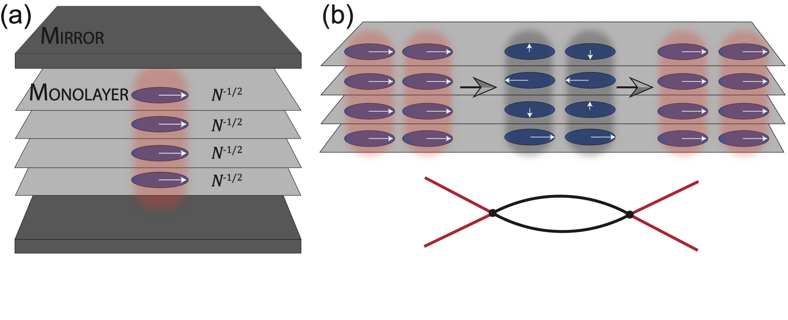
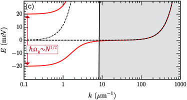
Figure 1: (a) Schematic illustration of the microcavity structure with $N$ embedded monolayers, where $N=4$. A polariton consists of a cavity photon (shaded red) and a superposition of $N$ in-phase 2D excitons (blue ellipses), where the relative phase of each exciton is represented by an in-plane arrow. (b) Example of a scattering process involving intermediate dark states which are uncoupled to light. (c) Polariton dispersion (red) at zero detuning, together with the uncoupled cavity photon and exciton modes (dashed black lines). For high momenta $k>\epsilon_{X}/\hbar c$ (shaded region), where $\epsilon_{X}$ is the exciton energy and $c$ is the speed of light, the exciton is far detuned in energy from the photon and thus essentially uncoupled. We use the parameters for MoSe₂ (see Table LABEL:tab) with $\epsilon_{X}=1.66$eV Dufferwiel et al. (2015) and $N=4$ layers.

The spin-degenerate eigenstates of Eq. (2) consist of two polariton modes (upper and lower branches) and $N-1$ dark states which are decoupled from light Ivchenko et al. (1994); Kavokin and Malpuech (2003). The multilayer system is frequently described by a two-coupled-mode exciton-photon model with a renormalized Rabi coupling Carusotto and Ciuti (2013), but here, we keep track of the complete structure of the eigenstates which is of crucial importance when we consider polariton interactions below. Since only the bright states [in-phase superpositions of all monolayer excitons, as depicted in Fig. 1(a)] couple to light, one can rewrite the Hamiltonian in the corresponding convenient basis:

$$\hat{H}_{0} = \sum_{\mathbf{k},\sigma}\left[E_{\mathbf{k}}^{C}\hat{c}_{\mathbf{k}\sigma}^{\dagger}\hat{c}_{\mathbf{k}\sigma}+E_{\mathbf{k}}^{X}\left(\hat{b}_{\mathbf{k}\sigma}^{\dagger}\hat{b}_{\mathbf{k}\sigma}+\sum_{l=1}^{N-1}\hat{d}_{\mathbf{k}\sigma,l}^{\dagger}\,\hat{d}_{\mathbf{k}\sigma,l}\right)\right]$$ (3)

$$+\frac{\hbar\Omega_{R}}{2}\sum_{\mathbf{k},\sigma}\left(\hat{b}_{\mathbf{k}\sigma}^{\dagger}\hat{c}_{\mathbf{k}\sigma}+\hat{c}_{\mathbf{k}\sigma}^{\dagger}\hat{b}_{\mathbf{k}\sigma}\right),$$

where $\hat{b}_{\mathbf{k}\sigma}$ and $\hat{d}_{\mathbf{k}\sigma,l}$ are the annihilation operators for bright and dark states, respectively, which are related to the bare monolayer exciton operators via the unitary transformation:

$$\hat{d}_{\mathbf{k}\sigma,l}=\sum_{n=1}^{N}u_{ln}\,\hat{x}_{\mathbf{k}\sigma,n},\leavevmode\nobreak\ \leavevmode\nobreak\ \hat{b}_{\mathbf{k}\sigma}\equiv\hat{d}_{\mathbf{k}\sigma,N}=\sum_{n=1}^{N}\frac{\hat{x}_{\mathbf{k}\sigma,n}}{\sqrt{N}}$$ (4)

with $u_{ln}=\frac{1}{\sqrt{N}}e^{i2\pi nl/N}$ . The multilayer nature of the bright states gives rise to an enhanced Rabi coupling $\hbar\Omega_{R}=\hbar g_{R}\sqrt{N}$, thus making it easier to access the strong-coupling regime in a multilayer structure. We emphasize that the present dark states consist of superpositions of monolayer bright excitons. Thus, they should not be confused with spin-forbidden dark excitons which can exist in free monolayers and have a different spectral energy Zhang et al. (2015); Wang et al. (2017).

The decomposition of the Hamiltonian into the basis of dark and bright excitons in Eq. (3) allows us to arrive at the diagonal form of the exciton-photon Hamiltonian:

$$\hat{H}_{0}=\!\sum_{\mathbf{k},\sigma}\!\left[E_{\mathbf{k}}^{L}\hat{L}_{\mathbf{k}\sigma}^{\dagger}\hat{L}_{\mathbf{k}\sigma}+E_{\mathbf{k}}^{U}\hat{U}_{\mathbf{k}\sigma}^{\dagger}\hat{U}_{\mathbf{k}\sigma}+\!\!\sum_{l=1}^{N-1}E_{\mathbf{k}}^{X}\hat{d}_{\mathbf{k}\sigma,l}^{\dagger}\hat{d}_{\mathbf{k}\sigma,l}\right]\!,$$

with $\hat{L}$ ($\hat{U}$) the lower (upper) polariton annihilation operators defined in the standard way

$$\begin{pmatrix}\hat{L}_{\mathbf{k}\sigma}\\ \hat{U}_{\mathbf{k}\sigma}\end{pmatrix}=\begin{pmatrix}X_{\mathbf{k}}&&C_{\mathbf{k}}\\ -C_{\mathbf{k}}&&X_{\mathbf{k}}\end{pmatrix}\begin{pmatrix}\hat{b}_{\mathbf{k}\sigma}\\ \hat{c}_{\mathbf{k}\sigma}\end{pmatrix}.$$ (5)

Here $E_{\mathbf{k}}^{U,L}$ are the polariton eigen-energies [see Fig. 1(c)],

$$E_{\mathbf{k}}^{U,L}=\frac{1}{2}\left(E_{\mathbf{k}}^{X}+E_{\mathbf{k}}^{C}\pm\sqrt{\left(E_{\mathbf{k}}^{C}-E_{\mathbf{k}}^{X}\right)^{2}+\hbar^{2}\Omega_{R}^{2}}\right),$$ (6)

and $X_{\mathbf{k}},C_{\mathbf{k}}$ are the Hopfield coefficients, corresponding to exciton and photon fractions:

$$X_{\mathbf{k}}^{2}=\frac{1}{2}\left(1+\frac{E_{\mathbf{k}}^{C}-E_{\mathbf{k}}^{X}}{E_{\mathbf{k}}^{U}-E_{\mathbf{k}}^{L}}\right),\leavevmode\nobreak\ \leavevmode\nobreak\ \leavevmode\nobreak\ C_{\mathbf{k}}^{2}=1-X_{\mathbf{k}}^{2}.$$ (7)

II.2 Exciton-exciton interactions

Since the layer spacing is typically larger than the exciton size, we may assume that the interactions between excitons only occur within the same layer. Furthermore, if the scattering energy is small compared to the exciton binding energy (as is the case in TMDs Wang et al. (2018)), then we can describe the exciton interactions with an $s$-wave contact potential,

$$\hat{V}=\sum_{n=1}^{N}\,\sum_{\begin{subarray}{c}{\bf k},{\bf k}^{\prime},{\bf q}\\ \sigma,\sigma^{\prime}\end{subarray}}\frac{g_{\sigma\sigma^{\prime}}}{2}\hat{x}_{\mathbf{k+q}\sigma,n}^{\dagger}\hat{x}_{\mathbf{k^{\prime}-q}\sigma^{\prime},n}^{\dagger}\hat{x}_{\mathbf{k^{\prime}}\sigma^{\prime},n}\hat{x}_{\mathbf{k}\sigma,n},$$ (8)

since at large separation the excitons have van der Waals interactions, which are short range Landau and Lifshitz (2013). The “bare” spin-dependent coupling strength $g_{\sigma\sigma^{\prime}}$ is independent of layer index $n$ since we have assumed that the monolayers are identical. Also, we have set the monolayer area to 1. Our approach is different from determining the exciton-exciton interaction strength within the Born approximation, as in previous works Ciuti et al. (1998); Tassone and Yamamoto (1999); Rochat et al. (2000); Combescot et al. (2008); Glazov et al. (2009); Shahnazaryan et al. (2017); Estrecho et al. (2019). That approximation effectively estimates $g_{\sigma\sigma^{\prime}}$ from the microscopic structure of the excitons, whereas here we solve the low-energy scattering problem exactly and treat $g_{\sigma\sigma^{\prime}}$ as a bare parameter that must be related to experimental observables Mora and Castin (2009). As such, we impose a cutoff $\Lambda$ on the relative scattering momentum, which we will send to infinity at the end of the calculation.

Transforming to the bright-dark exciton basis using Eq. (4), the interaction term becomes:

$$\hat{V}=\sum_{\{l_{j}\}}\delta_{\mathcal{M}}\!\!\sum_{\begin{subarray}{c}{\bf k},{\bf k}^{\prime},{\bf q}\\ \sigma,\sigma^{\prime}\end{subarray}}\frac{g_{\sigma\sigma^{\prime}}}{2N}\hat{d}_{\mathbf{k+q}\sigma,l_{1}}^{\dagger}\hat{d}_{\mathbf{k^{\prime}-q}\sigma^{\prime},l_{2}}^{\dagger}\hat{d}_{\mathbf{k^{\prime}}\sigma^{\prime},l_{3}}\hat{d}_{\mathbf{k}\sigma,l_{4}},$$ (9)

where $\{l_{j}\}=\{l_{1},l_{2},l_{3},l_{4}\}$. The kronecker delta ($\delta_{\mathcal{M}}=1$ if $\mathcal{M}=0$, $\delta_{\mathcal{M}}=0$ otherwise) encodes the phase selection rule for binary scatterings illustrated in Fig. 1(b), where $\mathcal{M}=\text{Mod}{[l_{1}+l_{2}-l_{3}-l_{4},N}]$. It is worth noting that the interaction coupling constant is reduced by the factor of $1/N$ in the new bright-dark-states basis. Moreover, written in this form, Eq. (9) can involve a huge number of terms ($N^{3}$ for each spin channel). This highlights the complexity of the scattering processes which can occur in any multilayer structure in the strong-coupling regime.

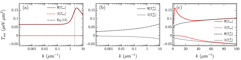
Figure 2: Polariton and exciton triplet elastic scattering as a function of relative momentum. (a) Real and imaginary parts of the full polariton $T$ matrix, Eq. (12), together with the analytical formula in the small photon mass approximation, Eq. (15). (b) Low-energy exciton triplet $T$ matrix, $T_{\sigma\sigma}^{X}(k)$, Eq. (46). (c) Polariton and exciton $T$ matrices on a larger momentum scale. We use the MoSe₂ parameters with $m_{X}=1.14m_{0}$ Kylänpää and Komsa (2015), $m_{C}=10^{-5}m_{0}$ Tan et al. (2020), $\delta=0$, and $N=1$, giving the inflection wave vector $q_{0}\simeq 2.29\mu$m^-1 [thin vertical line in panels (a,c)].

III Polariton-polariton scattering

To investigate polariton-polariton interations, we consider the two-body scattering problem at zero center-of-mass momentum. The two-particle states are $\ket{A_{\sigma},B_{\sigma^{\prime}},\mathbf{k}}=\hat{A}_{-\mathbf{k}\sigma}^{\dagger}\hat{B}_{\mathbf{k}\sigma^{\prime}}^{\dagger}\ket{0}$, where the operators $\hat{A}$, $\hat{B}$ can correspond to lower polaritons $\hat{L}$, upper polaritons $\hat{U}$ or dark-exciton operators $\hat{d}_{l}$, with $l=1,2,\ldots,N-1$. To proceed, we employ the $T$-matrix operator, which is given by the Born series

$$\hat{T}(E)=\hat{V}+\hat{V}\frac{1}{E-\hat{H}_{0}+i0}\hat{V}+...$$ (10)

where $E$ is the scattering energy and $+i0$ represents an infinitesimal positive imaginary part. The interaction strength for lower polaritons is then given by the matrix element

$$T_{\sigma\sigma^{\prime}}(k) \equiv\frac{\bra{L_{\sigma},L_{\sigma^{\prime}},\mathbf{k}^{\prime}}\hat{T}\!\left(2E_{\bf k}^{L}\right)\ket{L_{\sigma},L_{\sigma^{\prime}},\mathbf{k}}}{1+\delta_{\sigma\sigma^{\prime}}},$$ (11)

with the on-shell condition $|\mathbf{k}^{\prime}|=|\mathbf{k}|=k$. Here the normalization factor in the denominator accounts for scattering between identical particles. The Born approximation to the interaction strength corresponds to keeping only the first term in the series, which gives $g_{\sigma\sigma^{\prime}}X^{4}_{\bf k}/N$. However, higher order terms will significantly modify this result since they can involve scattering into dark intermediate states, as illustrated in Fig. 1(b).

Remarkably, we find that the low-energy polariton $T$ matrix takes the simple form (see Appendix A for the detailed calculation)

$$T_{\sigma\sigma^{\prime}}(k) =\frac{X_{\mathbf{k}}^{4}}{\frac{N}{g_{\sigma\sigma^{\prime}}}-\Pi\left(2E_{\bf k}^{L}\right)}.$$ (12)

Here, the one-loop polarization bubble $\Pi(E)$ is extremely well approximated by that of $N$ exciton pairs:

$$\Pi(E)\simeq N\sum_{\mathbf{q}}^{\Lambda}\frac{1}{E-2E_{\mathbf{q}}^{X}+i0},$$ (13)

since the exciton scattering is dominated by large momenta where the photon is far off resonant [see Fig. 1(c)]. This is a consequence of the small photon-exciton mass ratio, $m_{C}/m_{X}\simeq 10^{-5}$ (See Appendix B).

To obtain cutoff-independent results, we relate the bare couplings to physical observables as follows Levinsen and Parish (2015)

$$\frac{1}{g_{\sigma\sigma^{\prime}}}=-\sum_{\mathbf{q}}^{\Lambda}\frac{1}{\varepsilon_{\sigma\sigma^{\prime}}+2E_{\mathbf{q}}^{X}},$$ (14)

where we have introduced the physical energy scales $\varepsilon_{\sigma\sigma^{\prime}}=\frac{\hbar^{2}}{2m_{r}a_{\sigma\sigma^{\prime}}^{2}}$ related to the 2D exciton $s$-wave scattering lengths $a_{\sigma\sigma^{\prime}}$ and the two-exciton reduced mass $m_{r}=m_{X}/2$. Note that the scattering parameters are intrinsic to the monolayer and are independent of $N$. In the singlet case, $\varepsilon_{+-}=\varepsilon_{-+}=\varepsilon_{B}^{XX}$ corresponds to the binding energy of the biexciton (bound state of two excitons). Due to Pauli exclusion, there is no triplet biexciton state, but the triplet scattering length is well defined and is of the order of the 2D exciton Bohr radius $a_{\sigma\sigma}\sim a_{B}$ (See Appendix C); hence we have $\varepsilon_{\sigma\sigma}\sim\varepsilon_{B}^{X}$.

Inserting Eq. (14) into Eq. (12) and taking the limit $\Lambda\rightarrow\infty$, one obtains the cutoff-independent $T$ matrix

$$T_{\sigma\sigma^{\prime}}(k)=\frac{4\pi\hbar^{2}X_{\mathbf{k}}^{4}}{m_{X}N\ln\left(\frac{\varepsilon_{\sigma\sigma^{\prime}}}{2|E_{\mathbf{k}}^{L}|}\right)}.$$ (15)

The limit $k\rightarrow 0$ finally yields $T_{\sigma\sigma^{\prime}}$ in Eq. (1), which gives the lower polariton effective interaction “constants” for the triplet ($\alpha_{1}$) and singlet ($\alpha_{2}$) channels. Equations (1) and (15) show that the low-momentum polariton interaction strength is enhanced compared to that of monolayer excitons because the scattering energy is dominated by the strong light-matter coupling — for a detailed comparison, see the subsections III.2 and III.1 below. This is in sharp contrast to the behavior predicted by the Born approximation Ciuti et al. (1998); Tassone and Yamamoto (1999); Carusotto and Ciuti (2013). Furthermore, Eq. (1) implies that the chemical potential of a polariton condensate will scale linearly with density. This is consistent with recent measurements of the polariton blueshift in the Thomas Fermi regime Estrecho et al. (2019), and differs from the behavior of a 2D exciton condensate, which will feature a logarithmic dependence on density according to Bogoliubov theory Popov (1972); Mora and Castin (2009).

III.1 Comparison between exciton-exciton and polariton-polariton scattering

Equations (1) and (15) are key results of this work, since they imply that the low-momentum polariton interaction strength is enhanced compared to that of monolayer excitons, which is in sharp contrast to the behavior predicted by the Born approximation Ciuti et al. (1998); Tassone and Yamamoto (1999); Carusotto and Ciuti (2013). To see this, note that in the absence of light-matter coupling, Eq. (15) reduces to the usual 2D two-body $T$ matrix for quantum particles in a monolayer Adhikari (1986),

$$T^{X}_{\sigma\sigma^{\prime}}(k)=\frac{4\pi\hbar^{2}}{m_{X}}\frac{1}{\ln\left(\frac{\varepsilon_{\sigma\sigma^{\prime}}}{2E_{\mathbf{k}}^{X}}\right)+i\pi},$$ (16)

which describes the interactions of excitons. In Fig. 4 we compare the momentum dependence of the low-energy triplet polariton and exciton $T$ matrices for parameters corresponding to a MoSe₂ monolayer (see Table LABEL:tab). Crucially, we see that the strength of polariton-polariton elastic scattering, $T_{\sigma\sigma}$, is larger than the exciton-exciton one, $T_{\sigma\sigma}^{X}$, despite the presence of the Hopfield factor $X_{\bf k}^{4}$ in Eq. (15). By comparing Eqs. (15) with (46), we see that this enhancement of interactions is purely driven by the difference in scattering energy, which in turn is dominated by the strong light-matter Rabi coupling.

Apart from the enhancement due to the strong light-matter coupling, Fig. 4 shows that the polariton interactions behave qualitatively differently to exciton interactions. At small momenta, the polariton interactions are strongly affected by the Hopfield-factor momentum dependence, and hence the elastic interaction strength initially increases until it reaches a maximum slightly above the inflection wave vector $q_{0}$ of the non-parabolic polariton dispersion. At large wave vectors, the polariton scattering decreases, until it becomes exciton-like and recovers the standard behavior of 2D scattering, as shown in Fig. 4(c).

We emphasize that the peak in the polariton scattering $T$ matrix at finite relative momentum is not due to so-called optical parametric scattering. The present maximum is for scattering at zero total momentum whereas optical parametric scattering requires a finite total momentum $\sim 2q_{0}$.

For completeness, in Fig. 4(a) we display the results from the exact expression for polariton-polariton scattering, Eq. (12), as well as the analytic approximation in Eq. (15) which relied on the fact that $m_{C}/m_{X}\ll 1$ (dot-dashed black line). We see that these perfectly match for the relevant wave vectors probed in optical experiments, thus proving the validity of our approximations.

III.2 Polariton interactions at low momentum

Equation (46) indicates that the exciton interactions vanish logarithmically in the limit of zero momentum. By contrast, this behavior is absent for the polariton interactions shown in Fig. 4. However, in principle the 2D polariton $T$ matrix must vanish in the limit of strictly zero momentum, as is the case for any scattering of 2D quantum particles with short-range interactions. As we now explain, this strong qualitative difference between exciton and polariton interactions at very small momentum arises from the large exciton-photon mass ratio, since this implies that the typical momentum at which the polariton interactions start to approach zero is not resolvable in realistic experiments.

We obtained the analytical expression (15) by using the approximation (13), which amounts to replacing the polariton one-loop polarization bubble by the exciton one, as justified in Appendix B. From Eq. (44) with $E=2E_{\bf k}^{L}$ one can see that the leading correction to Eq. (13) at small momentum comes from the first term in the bracket, since this diverges in the zero-momentum limit:

$$\mathcal{A}=\frac{m_{L}}{4\pi\hbar^{2}}X_{0}^{4}\ln{\left(\frac{2E_{0}^{L}-E}{-E}\right)},$$ (17)

where $m_{L}=m_{C}/C_{0}^{2}$ is the lower polariton effective mass. Keeping this term, the $T$ matrix takes the form:

$$T_{\sigma\sigma^{\prime}}(k\rightarrow 0) \simeq \frac{X_{\mathbf{k}}^{4}}{\frac{N}{g_{\sigma\sigma^{\prime}}}-N\Pi_{X}\left(2E_{\bf k}^{L}\right)-\mathcal{A}}$$

$$= \frac{4\pi\hbar^{2}X_{\mathbf{k}}^{4}}{m_{X}N\ln{\left(\frac{\varepsilon_{\sigma\sigma^{\prime}}}{-2E_{\bf k}^{L}}\right)-m_{L}\ln{\left(\frac{2E_{0}^{L}-2E_{\bf k}^{L}}{-2E_{\bf k}^{L}}\right)X_{0}^{4}}}},$$

and indeed vanishes as

$$T_{\sigma\sigma^{\prime}}\xrightarrow[k\rightarrow 0]{}\frac{4\pi\hbar^{2}}{m_{L}\ln{\left(\frac{2|E_{0}^{L}|m_{L}}{-\hbar^{2}k^{2}}\right)}}.$$ (19)

One can estimate the wave vector at which this logarithmic behavior starts to dominate by comparing the two terms in the denominator in (48). Using the fact that $\ln{\left(\frac{\varepsilon_{\sigma\sigma^{\prime}}}{2|E_{0}^{L}|}\right)}\sim 1$, the second term becomes relevant when

$$k^{*}a_{\sigma\sigma^{\prime}}\sim\sqrt{\frac{m_{L}}{m_{X}}}e^{-\frac{Nm_{X}}{2m_{L}X_{0}^{4}}}\sim e^{-\frac{Nm_{X}}{m_{C}}},$$ (20)

where we have dropped the prefactor and removed the Hopfield coefficients of order 1 in the last term. Because of the large exciton-photon mass ratio, $k^{*}$ is extremely small. For example for $m_{X}/m_{C}=10^{4}$ and $N=1$, one gets $1/k^{*}\sim 10^{4343}a_{\sigma\sigma^{\prime}}$, corresponding to a length scale much larger than the observable universe radius ($\sim 4.4\times 10^{26}$m)! This explains why the vanishing of 2D polariton scattering at low momentum is unobservable in any experiment.

It is worth noting that the above estimate strongly differs from the case of binary collisions between ultracold bosonic atoms in quasi-2D geometries Petrov and Shlyapnikov (2001), for which the logarithmic behavior, albeit challenging to probe experimentally, is not physically impossible to reach.

IV Implications for experiments

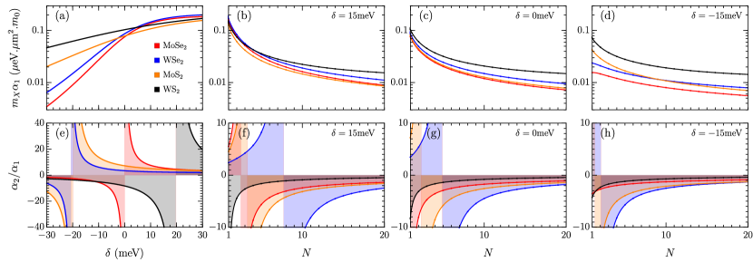
Figure 3: Polariton interactions in several 2D materials. (a,e) Monolayer triplet interactions $\alpha_{1}$ and the corresponding singlet-triplet ratio $\alpha_{2}/\alpha_{1}$ as a function of the exciton-photon detuning $\delta$. (b-d) Multilayer triplet interactions as a function of $N$ for different $\delta$, and (f-h) the corresponding singlet-triplet ratio. Parameters are taken from Table LABEL:tab, with $m_{0}$ the free electron mass.

We expect Eq. (1) to be accurate for TMD layers due to the sizeable exciton binding energies (see Table LABEL:tab) which imply that $|E_{0}^{L}|\ll\varepsilon_{B}^{X}$. Figure 3(a-d) show the polariton triplet interaction strength $\alpha_{1}$ for a range of photon-exciton detunings $\delta$ in different 2D TMD systems. Similar to previous predictions within the Born approximation, we find that $\alpha_{1}$ is repulsive and increases with increasing $\delta$ (corresponding to an increasing exciton fraction $X_{0}^{2}$). However, we see that a larger number of layers $N$ typically suppresses the polariton triplet interaction strength by a factor of $\sim N$ plus logarithmic corrections, suggesting that the strongest interactions occur in monolayer TMDs, while the largest Rabi coupling is achieved with multiple layers. For the case of monolayer MoSe₂, the value of $\alpha_{1}$ at detuning $\delta\simeq-15$meV is consistent with the recent low-density measurement reported in Ref. Tan et al. (2020) ($\alpha_{1}\simeq 0.01\mu$eV.$\mu$m²), thus confirming the validity of our model.

In contrast to the triplet case, the polariton singlet interaction strength $\alpha_{2}$ can display a scattering resonance when $2|E_{0}^{L}|\approx\varepsilon_{+-}$, corresponding to the point where the lower polariton branch crosses the biexciton energy. Such resonances are present in Fig. 3(e-h), where we have plotted the singlet/triplet ratio ($\alpha_{2}/\alpha_{1}$) for each TMD system. Here we see that the magnitude and even the sign of $\alpha_{2}$ can be tuned by varying $\delta$ and/or $N$. Furthermore, these panels demonstrate that the singlet interaction is in general stronger than the triplet one for a wide range of experimental parameters. To our knowledge, this important feature has not been noticed previously. In particular, a large and negative $\alpha_{2}/\alpha_{1}$ can destabilize a polariton condensate, which possibly explains why condensation has been challenging to achieve thus far. Based on current experimental data (Table LABEL:tab), our results in Fig. 3(e-h) suggest that WSe₂ is the most promising candidate for achieving condensation since it is easiest to access a regime with $\alpha_{2}>0$. Furthermore, the sizeable and tunable $\alpha_{2}$ in TMDs opens up the possibility of realizing strongly correlated phenomena such as polariton blockade Carusotto et al. (2010), bipolariton superfluidity Marchetti and Keeling (2014) and polaron physics Levinsen et al. (2019).

Thus far, we have focussed our discussion on the case of TMDs, where the large exciton binding energies mean that Eq. (1) is immediately applicable. In conventional quantum well semiconductor microcavities, the ratio of Rabi coupling to exciton binding energy is somewhat larger. For instance, in the case of a single GaAs quantum well, the ratio $\hbar\Omega_{R}/\varepsilon_{B}^{X}\simeq 0.35$, and therefore we still expect that our results are reasonably accurate at a quantitative level. Equation (1) then implies that the singlet interaction should be dominant, given the proximity to the biexciton resonance. Indeed this is consistent with experimental results, since the biexciton resonance has only been probed in single GaAs quantum well structures Takemura et al. (2014); Vladimirova et al. (2010); Takemura et al. (2017). We note that the enhancement of $\alpha_{2}$ in this context, known as the polariton “Feshbach resonance”, was proposed in Ref. Wouters (2007). On the other hand, for multiple quantum wells, such as structures with 12 layers, the Rabi coupling is comparable to the exciton binding energy Estrecho et al. (2019). While this means that we are formally outside the regime of validity of Eq. (1), we may still draw some qualitative conclusions based on this equation. In particular, from Eq. (1) we see that the enhanced Rabi coupling due to the multiple quantum wells means that the biexciton resonance is off resonant, and therefore the triplet interaction should dominate. This is also consistent with experiment — indeed in experiments with multiple quantum wells the singlet interaction is typically ignored Estrecho et al. (2019).

The singlet resonance effectively corresponds to the polariton “Feshbach resonance” Wouters (2007) experimentally investigated in single GaAs quantum wells Takemura et al. (2014, 2017). For TMDs, the resonance width is larger because of the larger biexciton binding energy; thus, it should be easier to resolve experimentally. We note that GaAs-based microcavities appear to be qualitatively different from the TMD case since values $|\alpha_{2}|/\alpha_{1}<1$ have been reported at negative detunings Vladimirova et al. (2010), below the biexciton resonance. Moreover, the exciton binding energy in these systems is not necessarily the largest energy scale — for example, for the case of 12 quantum wells, we have $\hbar\Omega_{R}\gtrsim\varepsilon_{B}^{X}$ Estrecho et al. (2019). However, Eq. (1) and our prediction of enhanced polariton interactions should be qualitatively applicable to quantum wells.

Note, though, that neither TMDs nor GaAs quantum wells are expected to feature a triplet polariton Feshbach resonance since there is no biexciton in this case: While Eq. (1) naively predicts a resonance at $2|E_{0}^{L}|\simeq\varepsilon_{B}^{X}$, such a large energy scale goes beyond the validity of our model and requires a more precise description of the short-distance physics such as the composite nature of the excitons and the layer thickness. A full microscopic description of such details is beyond the scope of the present work.

We emphasize that most of the intermediate states appearing in the $T$ matrix are dark states [Fig. 1(b)] which lie at the exciton energy. In our calculation, these correspond to virtual states that only contribute to the final strength of polariton interactions. However, in principle they can be turned into real long-lived excitons via additional scattering processes, for example mediated by phonons Piermarocchi et al. (1996); Savenko et al. (2013); Stepanov et al. (2019), and they can therefore populate an excitonic reservoir. Furthermore, to our knowledge, spontaneous polariton condensation has never been observed in single-quantum-well microcavities, which suggests that these dark states might also play an important role in the condensation process routinely reported in multi-quantum-well structures Kasprzak et al. (2006); Balili et al. (2007); Lagoudakis et al. (2008).

Finally, the finite value of zero-momentum polariton interactions given by Eq. (1) implies that the chemical potential of a polariton condensate will scale linearly with density. This is consistent with recent measurements of the polariton blueshift in the Thomas Fermi regime Estrecho et al. (2019), and differs from the behavior of a 2D exciton condensate, which will feature a logarithmic dependence on density according to Bogoliubov theory Popov (1972); Mora and Castin (2009). Such a logarithmic dependence has already been observed in condensates of paired fermionic atoms in quasi-2D geometries Boettcher et al. (2016).

V Summary and conclusions

We have derived exact analytical expressions for the polariton-polariton triplet and singlet interaction strengths in TMD layers embedded in a planar microcavity. Crucially, we have demonstrated that the strong exciton-photon coupling enhances the polariton interactions relative to those of bare excitons. The present work, together with the recent demonstration of the enhancement of polariton-electron scattering within a microscopic theory Li et al. (2020a, b), suggest that such strengthening of interactions induced by the strong light-matter coupling is a universal phenomenon in these systems, which has been unnoticed so far.

Furthermore, we have analyzed the dependence on the number of layers and we have exposed the important role of optically dark states in multilayer polariton-polariton scattering. Our results suggest that the singlet interaction is stronger than the triplet one for a range of TMD heterostructures, which has important consequences for realizing polariton condensation and other interaction-driven phenomena in these systems. In particular, a large repulsive singlet interaction can lead to the formation of spin-polarized domains, and thus to spin-resolved ultra-low threshold lasing.

Note added in proof.

After submission of this manuscript, a related work appeared in which a zero-temperature scalar polariton condensate in a monolayer system was theoretically investigated using a Bogoliubov approach, leading to a similar expression for $\alpha_{1}$ Hu et al. (2020).

SUPPLEMENTAL MATERIAL: “Polariton interactions in microcavities with atomically thin semiconductor layers”

Olivier Bleu, Guangyao Li, Jesper Levinsen, Meera M. Parish

School of Physics and Astronomy, Monash University, Victoria 3800, Australia and

ARC Centre of Excellence in Future Low-Energy Electronics Technologies, Monash University, Victoria 3800, Australia

Appendix A Polariton $T$-matrix

Here, we provide some details of the $T$-matrix calculation for the scattering between two lower polaritons. First, we recall the bosonic commutation rules:

$$\left[\hat{A}_{\mathbf{k}\sigma},\hat{B}_{\mathbf{k}^{\prime}\sigma^{\prime}}^{\dagger}\right]=\delta_{AB}\delta_{\sigma\sigma^{\prime}}\delta_{\mathbf{k}\mathbf{k}^{\prime}},$$ (21)

where $\hat{A}$, $\hat{B}$ can correspond to lower polaritons $\hat{L}$, upper polaritons $\hat{U}$ or dark-exciton operators $\hat{d}_{l}$, with $l=1,2,\ldots,N-1$. The two-particle states with zero total momentum are defined as:

$$\ket{A_{\sigma},B_{\sigma^{\prime}},\mathbf{k}}=\hat{A}_{-\mathbf{k}\sigma}^{\dagger}\hat{B}_{\mathbf{k}\sigma^{\prime}}^{\dagger}\ket{0},$$ (22)

with the scalar product:

$$\braket{A_{\sigma_{1}},B_{\sigma_{1}^{\prime}},\mathbf{k}_{1}}{C_{\sigma_{2}},D_{\sigma_{2}^{\prime}},\mathbf{k}_{2}} = \bra{0}\hat{B}_{\mathbf{k}_{1}\sigma_{1}^{\prime}}\hat{A}_{-\mathbf{k}_{1}\sigma_{1}}\hat{C}_{-\mathbf{k}_{2}\sigma_{2}}^{\dagger}\hat{D}_{\mathbf{k}_{2}\sigma_{2}^{\prime}}^{\dagger}\ket{0}$$ (23)

$$= \delta_{BC}\delta_{AD}\delta_{\sigma_{1}^{\prime}\sigma_{2}}\delta_{\sigma_{1}\sigma_{2}^{\prime}}\delta_{\mathbf{k}_{1},-\mathbf{k}_{2}}+\delta_{BD}\delta_{AC}\delta_{\sigma_{1}\sigma_{2}}\delta_{\sigma_{1}^{\prime}\sigma_{2}^{\prime}}\delta_{\mathbf{k}_{1}\mathbf{k}_{2}}.$$ (24)

The non-interacting eigenvalues are given by

$$\hat{H}_{0}\ket{A_{\sigma},B_{\sigma^{\prime}},\mathbf{k}} = \sum_{J}\sum_{\mathbf{q},s}E_{\mathbf{q}}^{J}\hat{J}_{\mathbf{q}s}^{\dagger}\hat{J}_{\mathbf{q}s}\hat{A}_{-\mathbf{k}\sigma}^{\dagger}\hat{B}_{\mathbf{k}\sigma^{\prime}}^{\dagger}\ket{0}$$ (25)

$$= \left(E_{\mathbf{-k}}^{A}+E_{\mathbf{k}}^{B}\right)\hat{A}_{-\mathbf{k}\sigma}^{\dagger}\hat{B}_{\mathbf{k}\sigma^{\prime}}^{\dagger}\ket{0}$$ (26)

$$= \left(E_{\mathbf{-k}}^{A}+E_{\mathbf{k}}^{B}\right)\ket{A_{\sigma},B_{\sigma^{\prime}},\mathbf{k}},$$ (27)

where the sum on $J$ in the first line accounts for all the available single-particle energy states, and $E_{\bf q}^{J}\equiv E^{X}_{\bf q}$ for all the dark states with $\hat{J}=\hat{d}_{l}$.

Now we consider the scattering between two lower polaritons, the first term of the Born series gives:

$$\bra{L_{\sigma},L_{\sigma^{\prime}},\mathbf{k}^{\prime}}\hat{V}\ket{L_{\sigma},L_{\sigma^{\prime}},\mathbf{k}}=X_{\mathbf{k}^{\prime}}^{2}X_{\mathbf{k}}^{2}\frac{g_{\sigma\sigma^{\prime}}}{N}(1+\delta_{\sigma\sigma^{\prime}}).$$ (28)

(Notice that $g_{+-}=g_{-+}$, and $g_{++}=g_{--}$). Higher order terms in the $T$-matrix involve dark or upper polariton intermediate states. It is useful to introduce the matrix element between two lower polaritons and an arbitrary two-particle state

$$\bra{A_{\sigma},B_{\sigma^{\prime}},\mathbf{k}^{\prime}}\hat{V}\ket{L_{\sigma},L_{\sigma^{\prime}},\mathbf{k}}=\frac{g_{\sigma\sigma^{\prime}}X_{\mathbf{k}}^{2}}{N}(1+\delta_{\sigma\sigma^{\prime}})\begin{cases}\delta_{\text{Mod}[l_{1}+l_{2},N]},&A=d_{l_{1}},\leavevmode\nobreak\ B=d_{l_{2}},\leavevmode\nobreak\ \leavevmode\nobreak\ l_{1},l_{2}\neq N\\ X_{\mathbf{k}^{\prime}}^{2},&A=L,\leavevmode\nobreak\ B=L\\ C_{\mathbf{k}^{\prime}}^{2},&A=U,\leavevmode\nobreak\ B=U\\ -X_{\mathbf{k}^{\prime}}C_{\mathbf{k}^{\prime}},&A=L,\leavevmode\nobreak\ B=U\\ -X_{\mathbf{k}^{\prime}}C_{\mathbf{k}^{\prime}},&A=U,\leavevmode\nobreak\ B=L,\end{cases}$$ (29)

and the completeness relation

$$\mathbb{1}=\frac{1}{2}\sum_{\mathbf{q}}\sum_{A,B}\sum_{s,s^{\prime}}\ket{A_{s},B_{s^{\prime}},\mathbf{q}}\bra{A_{s},B_{s^{\prime}},\mathbf{q}},$$ (30)

which satisfies the usual property of the identity

$$\mathbb{1}\ket{C_{\sigma},D_{\sigma^{\prime}},\mathbf{k}} = \frac{1}{2}\sum_{\mathbf{q}}\sum_{A,B}\sum_{s,s^{\prime}}\ket{A_{s},B_{s^{\prime}},\mathbf{q}}\braket{A_{s},B_{s^{\prime}},\mathbf{q}}{C_{\sigma},D_{\sigma^{\prime}},\mathbf{k}}$$ (31)

$$= \frac{1}{2}\sum_{\mathbf{q}}\left(\ket{C_{\sigma},D_{\sigma^{\prime}},\mathbf{q}}\delta_{\mathbf{q}\mathbf{k}}+\ket{D_{\sigma^{\prime}},C_{\sigma},\mathbf{q}}\delta_{\mathbf{q},-\mathbf{k}}\right)$$ (32)

$$= \frac{1}{2}\left(\ket{C_{\sigma},D_{\sigma^{\prime}},\mathbf{k}}+\ket{D_{\sigma^{\prime}},C_{\sigma},-\mathbf{k}}\right)$$ (33)

$$= \ket{C_{\sigma},D_{\sigma^{\prime}},\mathbf{k}}.$$ (34)

Then the second-order term reads

$$\bra{L^{\sigma},L^{\sigma^{\prime}},\mathbf{k}^{\prime}}\hat{V}\frac{1}{E-\hat{H}_{0}}\hat{V}\ket{L^{\sigma},L^{\sigma^{\prime}},\mathbf{k}} = \bra{L^{\sigma},L^{\sigma^{\prime}},\mathbf{k}^{\prime}}\hat{V}\mathbb{1}\frac{1}{E-\hat{H}_{0}}\hat{V}\ket{L^{\sigma},L^{\sigma^{\prime}},\mathbf{k}}$$ (35)

$$= (1+\delta_{\sigma\sigma^{\prime}})\left(\frac{g_{\sigma\sigma^{\prime}}}{N}\right)^{2}X_{\mathbf{k}}^{2}X_{\mathbf{k}^{\prime}}^{2}$$

$$\times\sum_{\mathbf{q}}\left[\frac{X_{\mathbf{q}}^{4}}{E-2E_{\mathbf{q}}^{L}}+\frac{C_{\mathbf{q}}^{4}}{E-2E_{\mathbf{q}}^{U}}+\frac{2C_{\mathbf{q}}^{2}X_{\mathbf{q}}^{2}}{E-E_{\mathbf{q}}^{L}-E_{\mathbf{q}}^{U}}+\sum_{l_{1},l_{2}}^{N-1}\frac{\delta_{\text{Mod}[l_{1}+l_{2},N]}}{E-2E_{\mathbf{q}}^{X}}\right]$$

$$= (1+\delta_{\sigma\sigma^{\prime}})\frac{g_{\sigma\sigma^{\prime}}X_{\mathbf{k}}^{4}}{N}\frac{g_{\sigma\sigma^{\prime}}}{N}\Pi(E),$$ (37)

where we have used $|\mathbf{k}^{\prime}|=|\mathbf{k}|$ in the last line. The one-loop polarization bubble, $\Pi(E)$, is given by

$$\Pi(E) = \underbrace{\sum_{\mathbf{q}}^{\Lambda}\frac{X_{\mathbf{q}}^{4}}{E-2E_{\mathbf{q}}^{L}}+\sum_{\mathbf{q}}^{\Lambda}\frac{C_{\mathbf{q}}^{4}}{E-2E_{\mathbf{q}}^{U}}+2\sum_{\mathbf{q}}^{\Lambda}\frac{X_{\mathbf{q}}^{2}C_{\mathbf{q}}^{2}}{E-E_{\mathbf{q}}^{L}-E_{\mathbf{q}}^{U}}}_{\Pi_{P}(E)}+(N-1)\underbrace{\sum_{\mathbf{q}}^{\Lambda}\frac{1}{E-2E_{\mathbf{q}}^{X}}}_{\Pi_{X}(E)},$$ (38)

where we have introduced the high-energy cutoff wave vector $\Lambda$. Note that, had we dropped the dark states in Eq. (2) as is commonly done Carusotto and Ciuti (2013), the term $\left(N-1\right)\Pi_{X}$ would be absent. Hence the dark states play an essential role in the interactions.

The generalisation to higher order terms leads to

$$\bra{L_{\sigma},L_{\sigma^{\prime}},\mathbf{k}^{\prime}}\hat{T}(E)\ket{L_{\sigma},L_{\sigma^{\prime}},\mathbf{k}} = (1+\delta_{\sigma\sigma^{\prime}})\frac{g_{\sigma\sigma^{\prime}}X_{\mathbf{k}}^{4}}{N}\left[1+\frac{g_{\sigma\sigma^{\prime}}}{N}\Pi(E)+\left(\frac{g_{\sigma\sigma^{\prime}}}{N}\Pi(E)\right)^{2}+...\right]$$ (39)

$$= (1+\delta_{\sigma\sigma^{\prime}})\frac{X_{\mathbf{k}}^{4}}{\left(\frac{N}{g_{\sigma\sigma^{\prime}}}-\Pi(E)\right)},$$ (40)

which after rearranging the prefactor, gives the formula (12) presented in the main text. Note that $\Pi(E)$ also contains a factor $N$. The integrals in $\Pi(E)$ are dominated by the large wavectors $\mathbf{q}$, where $E_{\mathbf{q}}^{L}\rightarrow E_{\mathbf{q}}^{X}$, $X_{\mathbf{q}}^{2}\rightarrow 1$, $C_{\mathbf{q}}^{2}\rightarrow 0$ and one can neglect the second and third terms. Thus, $\Pi(E)$ simply reduces to $N\times\Pi_{X}(E)$. This approximation is valid because $m_{C}\ll m_{X}$ as explained below.

Appendix B $m_{C}\ll m_{X}$ and $\Pi(E)$ approximation

The approximation of the one-loop polarization bubble [Eq. (38)] relies on the very large difference between the cavity photon and the exciton masses ($m_{C}/m_{X}\sim 10^{-4}-10^{-5}$). This approximation is equivalent to neglecting the low-$q$ behavior of the integrand in:

$$\Pi_{P}(E)=\frac{1}{2\pi}\int_{0}^{\Lambda}qdq\left(\frac{X_{\mathbf{q}}^{4}}{E-2E_{\mathbf{q}}^{L}}+\frac{C_{\mathbf{q}}^{4}}{E-2E_{\mathbf{q}}^{U}}+2\frac{X_{\mathbf{q}}^{2}C_{\mathbf{q}}^{2}}{E-E_{\mathbf{q}}^{L}-E_{\mathbf{q}}^{U}}\right).$$ (41)

To analytically evaluate if this low-q behavior plays a role, one can approximate the integrand in two domains with the following replacements:

• $q<q_{0}$: $E_{\mathbf{q}}^{L}\rightarrow\tilde{E}_{\mathbf{q}}^{L}=\hbar^{2}q^{2}/2m_{L}+E_{0}^{L}$, $E_{\mathbf{q}}^{U}\rightarrow\tilde{E}_{\mathbf{q}}^{U}=\hbar^{2}q^{2}/2m_{U}+E_{0}^{U}$, $C_{\mathbf{q}}\rightarrow C_{0}$, $X_{\mathbf{q}}\rightarrow X_{0}$

• $q>q_{0}$: $E_{\mathbf{q}}^{L}\rightarrow E_{\mathbf{q}}^{X}$, $C_{\mathbf{q}}\rightarrow 0$, $X_{\mathbf{q}}\rightarrow 1$.

The inflection wave vector $q_{0}$ and the lower (upper) polariton effective masses $m_{L}$, ($m_{U}$) are defined as:

$$q_{0}=\frac{\sqrt{2m_{L}|E_{0}^{L}|}}{\hbar},\leavevmode\nobreak\ \leavevmode\nobreak\ m_{L}=\frac{m_{C}}{C_{0}^{2}},\leavevmode\nobreak\ \leavevmode\nobreak\ m_{U}=\frac{m_{C}}{X_{0}^{2}}.$$ (42)

This gives

$$\Pi_{P}(E) \simeq \frac{1}{2\pi}\int_{0}^{q_{0}}qdq\left(\frac{X_{0}^{4}}{E-2\tilde{E}_{\mathbf{q}}^{L}}+\frac{C_{0}^{4}}{E-2\tilde{E}_{\mathbf{q}}^{U}}+2\frac{X_{0}^{2}C_{0}^{2}}{E-\tilde{E}_{\mathbf{q}}^{L}-\tilde{E}_{\mathbf{q}}^{U}}\right)+\frac{1}{2\pi}\int_{q_{0}}^{\Lambda}qdq\left(\frac{1}{E-2E_{\mathbf{q}}^{X}}\right)$$ (44)

$$= \frac{m_{C}}{4\pi\hbar^{2}C_{0}^{2}X_{0}^{2}}\left[X_{0}^{6}\ln{\left(\frac{2E_{0}^{L}-E}{-E}\right)}+C_{0}^{6}\ln{\left(\frac{2E_{0}^{U}-E}{2E_{0}^{U}-E+2|E_{0}^{L}|X_{0}^{2}/C_{0}^{2}}\right)}+4X_{0}^{4}C_{0}^{4}\ln{\left(\frac{(\delta-E)C_{0}^{2}X_{0}^{2}}{C_{0}^{2}(\delta-E)+|E_{0}^{L}|}\right)}\right]$$

$$+\frac{m_{X}}{4\pi\hbar^{2}}\ln{\left(\frac{E-2|E_{0}^{L}|C_{0}^{2}m_{C}/m_{X}}{E-2E_{\Lambda}^{X}}\right)}$$

$$\simeq \frac{m_{X}}{4\pi\hbar^{2}}\ln{\left(\frac{E}{E-2E_{\Lambda}^{X}}\right)}=\sum_{\mathbf{q}}^{\Lambda}\frac{1}{E-2E_{\mathbf{q}}^{X}}.$$ (45)

Hence, one can see that in the limit $m_{C}/m_{X}\rightarrow 0$, $\Pi_{P}(E)\rightarrow\Pi_{X}(E)$, and Eq. (38) reduces to $\Pi(E)\simeq N\Pi_{X}(E)$.

Vanishing polariton interactions?

In the absence of light-matter coupling, we recover the usual 2D two-body $T$ matrix for quantum particles in a monolayer Adhikari (1986),

$$T^{X}_{\sigma\sigma^{\prime}}(k)=\frac{4\pi\hbar^{2}}{m_{X}}\frac{1}{\ln\left(\frac{\varepsilon_{\sigma\sigma^{\prime}}}{2E_{\mathbf{k}}^{X}}\right)+i\pi},$$ (46)

which describes the interactions of excitons. We see that this vanishes logarithmically in the limit of zero momentum. In principle the 2D polariton $T$ matrix should also vanish at strictly zero momentum. However, the typical momentum at which such behavior starts to be relevant is incredibly small and not resolvable in practice, as we now explain.

From Eq. (44) with $E=2E_{\bf k}^{L}$ one can see that the leading correction at small momentum comes from the first term in the bracket, since this diverges in the zero-momentum limit:

$$\mathcal{A}=\frac{m_{L}}{4\pi\hbar^{2}}X_{0}^{4}\ln{\left(\frac{2E_{0}^{L}-E}{-E}\right)}.$$ (47)

Keeping this term, the $T$ matrix takes the form:

$$T_{\sigma\sigma^{\prime}}(k\rightarrow 0)\simeq\frac{X_{\mathbf{k}}^{4}}{\frac{N}{g_{\sigma\sigma^{\prime}}}-N\Pi_{X}\left(2E_{\bf k}^{L}\right)-\mathcal{A}}=\frac{4\pi\hbar^{2}X_{\mathbf{k}}^{4}}{m_{X}N\ln{\left(\frac{\varepsilon_{\sigma\sigma^{\prime}}}{-2E_{\bf k}^{L}}\right)-m_{L}\ln{\left(\frac{2E_{0}^{L}-2E_{\bf k}^{L}}{-2E_{\bf k}^{L}}\right)X_{0}^{4}}}},$$ (48)

and indeed vanishes as

$$T_{\sigma\sigma^{\prime}}\xrightarrow[k\rightarrow 0]{}\frac{4\pi\hbar^{2}}{m_{L}\ln{\left(\frac{2|E_{0}^{L}|m_{L}}{-\hbar^{2}k^{2}}\right)}}.$$ (49)

One can estimate the wave vector at which this logarithmic behavior starts to dominate by comparing the two terms in the denominator in (48). Using the fact that $\ln{\left(\frac{\varepsilon_{\sigma\sigma^{\prime}}}{2|E_{0}^{L}|}\right)}\sim 1$, the second term becomes relevant when

$$k^{*}a_{\sigma\sigma^{\prime}}\sim\sqrt{\frac{m_{L}}{m_{X}e}}e^{-\frac{Nm_{X}}{2m_{L}X_{0}^{4}}}\sim e^{-\frac{Nm_{X}}{m_{C}}},$$ (50)

where we have dropped the prefactor and removed the Hopfield coefficients of order 1 in the last term. Because of the large exciton-photon mass ratio, $k^{*}$ is extremely small. For example for $m_{X}/m_{C}=10^{4}$ and $N=1$, one gets $1/k^{*}\sim 10^{4343}a_{\sigma\sigma^{\prime}}$, corresponding to a length scale much larger than the observable universe radius ($l_{u}=4.4\times 10^{26}$m)! This explains why the vanishing of 2D polariton scattering at low momentum is unobservable in any experiment.

Appendix C Triplet exciton-exciton scattering

In the main text, we assume that the exciton triplet scattering length is of the order of the exciton Bohr radius $a_{B}$. Here, we motivate this assumption by recalling that this is the case for 2D hard disk particles of radius $r_{0}$. For low-energy particles, the two-body scattering is dominated by the $s$ wave contribution, and the center of mass wavefunction obeys the 2D radial Schrödinger equation Landau and Lifshitz (2013)

$$-\frac{\hbar^{2}}{2m_{r}}\frac{1}{r}\frac{\partial}{\partial r}\left(r\frac{\partial\psi}{\partial r}\right)+U(r)\psi=E\psi,$$ (51)

with $m_{r}$ the two-body reduced mass. The hard disk potential corresponds to an infinitely high potential barrier of radius $r_{0}$

$$U=\begin{cases}\infty,\leavevmode\nobreak\ \leavevmode\nobreak\ r\leqslant r_{0}\\ 0,\leavevmode\nobreak\ \leavevmode\nobreak\ r>r_{0}.\end{cases}$$ (52)

Outside the potential, the general solution is a superposition of first and second kind Bessel functions

$$\psi(r)=AJ_{0}(kr)+BY_{0}(kr),$$ (53)

with $k=\sqrt{2m_{r}E}/\hbar$. Then, using its asymptotic form, one introduces the scattering phase shift $\delta_{s}$

$$\psi(r)\xrightarrow[r\rightarrow\infty]{}\sqrt{\frac{2}{\pi kr}}\left(A\cos(kr-\pi/4)+B\sin(kr-\pi/4)\right)=\sqrt{\frac{2}{\pi kr}}C\cos(kr-\pi/4+\delta_{s}),$$ (54)

with

$$\tan(\delta_{s})=-\frac{B}{A}.$$ (55)

The continuity of the wavefunction at $r=r_{0}$ gives the relation:

$$\cot\left(\delta_{s}\right)=-\frac{A}{B}=\frac{Y_{0}(kr_{0})}{J_{0}(kr_{0})}.$$ (56)

Finally, taking the low-energy (low-$k$) limit one obtains

$$\cot\left(\delta_{s}\right)=\frac{2}{\pi}\ln\left(ka_{s}\right),$$ (57)

where we have introduced the 2D scattering length $a_{s}$

$$a_{s}=\frac{e^{\gamma}r_{0}}{2}\simeq 0.89r_{0},$$ (58)

with $\gamma=0.577...$ the Euler-Mascheroni constant.

The corresponding hard disc triplet exciton $T$-matrix reads:

$$T_{\sigma\sigma}^{X}(k)=\frac{2\pi\hbar^{2}}{m_{r}}\left[\ln\left(\frac{\varepsilon_{\sigma\sigma}}{E}\right)+i\pi\right]^{-1},$$ (59)

with

$$\varepsilon_{\sigma\sigma}=\frac{\hbar^{2}}{2m_{r}a_{s}^{2}}.$$ (60)

Note that a similar form for the low-energy $T$ matrix has been obtained in Refs. Takayama et al. (2002); Schindler and Zimmermann (2008), both accounting for the composite (electron-hole) nature of the 2D excitons with different theoretical approaches. We emphasize that the exciton-exciton scattering vanishes only at zero momentum (see Fig. 4 (b,c)), and an arbitrary exciton momentum distribution (such as Maxwell-Boltzmann) necessarily leads to non-zero scattering. Hence, the above simple formula does not contradict the signatures of exciton-exciton interaction reported in experiments (such as in Ref. Moody et al. (2015)).

Appendix D Comparison between exciton-exciton and polariton-polariton scattering

Figures LABEL:figS1(a-b) show the momentum dependence for the low-energy polariton and exciton $T$ matrices with the parameters of a MoSe₂ monolayer. The $x$-axis is on a log scale to highlight the difference in the low-momentum behavior. Panel (a) displays the results from Eq. (12), as well as the analytic approximation in Eq. (15) which relied on the fact that $m_{C}/m_{X}\ll 1$ (dot-dashed black line). We see that these perfectly match for the relevant wave vectors probed in optical experiments. Crucially, we see that the polariton-polariton elastic scattering, $T_{\sigma\sigma}$, is larger than the exciton-exciton one, $T_{\sigma\sigma}^{X}$, despite the presence of the Hopfield factor $X_{\bf k}^{4}$ in Eqs. (12) and (15), and in particular $T_{\sigma\sigma}$ remains finite as $k\to 0$. Furthermore, its behavior is strongly affected by the Hopfield factor momentum dependence, and hence the elastic interaction strength initially increases until it reaches a maximum slightly above the inflection wave vector $q_{0}$ of the non-parabolic polariton dispersion.

Figure LABEL:figS1(c) shows the momentum dependence of both the polariton and exciton $T$ matrices on a larger scale (linear $x$-axis). We can see that at large wave vectors, the polariton scattering decreases, until it becomes exciton-like and recovers the standard behavior of 2D scattering.

We emphasize that the peak in the polariton scattering $T$ matrix at finite relative momentum is not due to so-called optical parametric scattering. The present maximum is for scattering at zero total momentum whereas optical parametric scattering requires a finite total momentum $\sim 2q_{0}$.

Figure 4: Polariton and exciton triplet elastic scattering as a function of relative momentum. (a) Real and imaginary parts of the full polariton $T$ matrix, Eq. (12) in the main text, together with the analytical formula in the small photon mass approximation, Eq. (15)in the main text. (b) Low-energy exciton triplet $T$ matrix, $T_{\sigma\sigma}^{X}(k)$, Eq. (46). (c) Polariton and exciton $T$ matrices on a larger momentum scale. We use the MoSe₂ parameters with $m_{X}=1.14m_{0}$ Kylänpää and Komsa (2015), $m_{C}=10^{-5}m_{0}$ Tan et al. (2020), $\delta=0$, and $N=1$, giving the inflection wave vector $q_{0}\simeq 2.29\mu$m^-1 [thin vertical line in panels (a,c)].

References

- Savvidis et al. (2000) P. G. Savvidis, J. J. Baumberg, R. M. Stevenson, M. S. Skolnick, D. M. Whittaker, and J. S. Roberts, Angle-Resonant Stimulated Polariton Amplifier, Phys. Rev. Lett. 84, 1547 (2000).
- Baas et al. (2004) A. Baas, J. P. Karr, H. Eleuch, and E. Giacobino, Optical bistability in semiconductor microcavities, Phys. Rev. A 69, 023809 (2004).
- Kasprzak et al. (2006) J. Kasprzak, M. Richard, S. Kundermann, A. Baas, P. Jeambrun, J. M. J. Keeling, F. M. Marchetti, M. H. Szymańska, R. André, J. L. Staehli, V. Savona, P. B. Littlewood, B. Deveaud, and L. S. Dang, Bose-Einstein condensation of exciton polaritons, Nature 443, 409 (2006).
- Balili et al. (2007) R. Balili, V. Hartwell, D. Snoke, L. Pfeiffer, and K. West, Bose-Einstein Condensation of Microcavity Polaritons in a Trap, Science 316, 1007 (2007).
- Amo et al. (2009) A. Amo, J. Lefrère, S. Pigeon, C. Adrados, C. Ciuti, I. Carusotto, R. Houdré, E. Giacobino, and A. Bramati, Superfluidity of polaritons in semiconductor microcavities, Nature Physics 5, 805 (2009).
- Lagoudakis et al. (2008) K. G. Lagoudakis, M. Wouters, M. Richard, A. Baas, I. Carusotto, R. André, L. S. Dang, and B. Deveaud-Plédran, Quantized vortices in an exciton-polariton condensate, Nature Physics 4, 706 (2008).
- Keeling et al. (2007) J. Keeling, F. M. Marchetti, M. H. Szymańska, and P. B. Littlewood, Collective coherence in planar semiconductor microcavities, Semiconductor Science and Technology 22, R1 (2007).
- Deng et al. (2010) H. Deng, H. Haug, and Y. Yamamoto, Exciton-polariton Bose-Einstein condensation, Rev. Mod. Phys. 82, 1489 (2010).
- Carusotto and Ciuti (2013) I. Carusotto and C. Ciuti, Quantum fluids of light, Rev. Mod. Phys. 85, 299 (2013).
- Kavokin et al. (2017) A. Kavokin, J. J. Baumberg, G. Malpuech, and F. P. Laussy, Microcavities (Oxford university press, 2017).
- He et al. (2014) K. He, N. Kumar, L. Zhao, Z. Wang, K. F. Mak, H. Zhao, and J. Shan, Tightly Bound Excitons in Monolayer , Phys. Rev. Lett. 113, 026803 (2014).
- Ye et al. (2014) Z. Ye, T. Cao, K. O’Brien, H. Zhu, X. Yin, Y. Wang, S. G. Louie, and X. Zhang, Probing excitonic dark states in single-layer tungsten disulphide, Nature 513, 214 (2014).
- Chernikov et al. (2014) A. Chernikov, T. C. Berkelbach, H. M. Hill, A. Rigosi, Y. Li, O. B. Aslan, D. R. Reichman, M. S. Hybertsen, and T. F. Heinz, Exciton Binding Energy and Nonhydrogenic Rydberg Series in Monolayer , Phys. Rev. Lett. 113, 076802 (2014).
- Wang et al. (2018) G. Wang, A. Chernikov, M. M. Glazov, T. F. Heinz, X. Marie, T. Amand, and B. Urbaszek, Colloquium: Excitons in atomically thin transition metal dichalcogenides, Rev. Mod. Phys. 90, 021001 (2018).
- Mikhnenko et al. (2015) O. V. Mikhnenko, P. W. M. Blom, and T.-Q. Nguyen, Exciton diffusion in organic semiconductors, Energy Environ. Sci. 8, 1867 (2015).
- Sanvitto and Kéna-Cohen (2016) D. Sanvitto and S. Kéna-Cohen, The road towards polaritonic devices, Nature Materials 15, 1061 (2016).
- Liu et al. (2014) X. Liu, T. Galfsky, Z. Sun, F. Xia, E.-c. Lin, Y.-H. Lee, S. Kéna-Cohen, and V. M. Menon, Strong light–matter coupling in two-dimensional atomic crystals, Nature Photonics 9, 30 (2014).
- Flatten et al. (2016) L. C. Flatten, Z. He, D. M. Coles, A. A. P. Trichet, A. W. Powell, R. A. Taylor, J. H. Warner, and J. M. Smith, Room-temperature exciton-polaritons with two-dimensional WS2, Scientific Reports 6, 33134 (2016).
- Lundt et al. (2016) N. Lundt, S. Klembt, E. Cherotchenko, S. Betzold, O. Iff, A. V. Nalitov, M. Klaas, C. P. Dietrich, A. V. Kavokin, S. Höfling, and C. Schneider, Room-temperature Tamm-plasmon exciton-polaritons with a WSe2 monolayer, Nature Communications 7, 13328 (2016).
- Sidler et al. (2017) M. Sidler, P. Back, O. Cotlet, A. Srivastava, T. Fink, M. Kroner, E. Demler, and A. Imamoglu, Fermi polaron-polaritons in charge-tunable atomically thin semiconductors, Nature Physics 13, 255 (2017).
- Dufferwiel et al. (2015) S. Dufferwiel, S. Schwarz, F. Withers, A. A. P. Trichet, F. Li, M. Sich, O. Del Pozo-Zamudio, C. Clark, A. Nalitov, D. D. Solnyshkov, G. Malpuech, K. S. Novoselov, J. M. Smith, M. S. Skolnick, D. N. Krizhanovskii, and A. I. Tartakovskii, Exciton-polaritons in van der Waals heterostructures embedded in tunable microcavities, Nature Communications 6, 8579 (2015).
- Król et al. (2019) M. Król, K. Rechcińska, K. Nogajewski, M. Grzeszczyk, K. Łempicka, R. Mirek, S. Piotrowska, K. Watanabe, T. Taniguchi, M. R. Molas, M. Potemski, J. Szczytko, and B. Pietka, Exciton-polaritons in multilayer WSe 2 in a planar microcavity, 2D Materials 7, 015006 (2019).
- Schneider et al. (2018) C. Schneider, M. M. Glazov, T. Korn, S. Höfling, and B. Urbaszek, Two-dimensional semiconductors in the regime of strong light-matter coupling, Nature Communications 9, 2695 (2018).
- Geim and Grigorieva (2013) A. K. Geim and I. V. Grigorieva, Van der Waals heterostructures, Nature 499, 419 (2013).
- Shelykh et al. (2009) I. A. Shelykh, A. V. Kavokin, Y. G. Rubo, T. C. H. Liew, and G. Malpuech, Polariton polarization-sensitive phenomena in planar semiconductor microcavities, Semiconductor Science and Technology 25, 013001 (2009).
- Scuri et al. (2018) G. Scuri, Y. Zhou, A. A. High, D. S. Wild, C. Shu, K. De Greve, L. A. Jauregui, T. Taniguchi, K. Watanabe, P. Kim, M. D. Lukin, and H. Park, Large Excitonic Reflectivity of Monolayer Encapsulated in Hexagonal Boron Nitride, Phys. Rev. Lett. 120, 037402 (2018).
- Barachati et al. (2018) F. Barachati, A. Fieramosca, S. Hafezian, J. Gu, B. Chakraborty, D. Ballarini, L. Martinu, V. Menon, D. Sanvitto, and S. Kéna-Cohen, Interacting polariton fluids in a monolayer of tungsten disulfide, Nature Nanotechnology 13, 906 (2018).
- Tan et al. (2020) L. B. Tan, O. Cotlet, A. Bergschneider, R. Schmidt, P. Back, Y. Shimazaki, M. Kroner, and A. m. c. İmamoğlu, Interacting Polaron-Polaritons, Phys. Rev. X 10, 021011 (2020).
- Emmanuele et al. (2020) R. P. A. Emmanuele, M. Sich, O. Kyriienko, V. Shahnazaryan, F. Withers, A. Catanzaro, P. M. Walker, F. A. Benimetskiy, M. S. Skolnick, A. I. Tartakovskii, I. A. Shelykh, and D. N. Krizhanovskii, Highly nonlinear trion-polaritons in a monolayer semiconductor, Nature Communications 11, 3589 (2020).
- Gu et al. (2019) J. Gu, V. Walther, L. Waldecker, D. Rhodes, A. Raja, J. C. Hone, T. F. Heinz, S. Kena-Cohen, T. Pohl, and V. M. Menon, Enhanced nonlinear interaction of polaritons via excitonic Rydberg states in monolayer WSe2 (2019), arXiv:1912.12544 [cond-mat.mtrl-sci] .
- Waldherr et al. (2018) M. Waldherr, N. Lundt, M. Klaas, S. Betzold, M. Wurdack, V. Baumann, E. Estrecho, A. Nalitov, E. Cherotchenko, H. Cai, E. A. Ostrovskaya, A. V. Kavokin, S. Tongay, S. Klembt, S. Höfling, and C. Schneider, Observation of bosonic condensation in a hybrid monolayer MoSe2-GaAs microcavity, Nature Communications 9, 3286 (2018).
- Takayama et al. (2002) R. Takayama, N. H. Kwong, I. Rumyantsev, M. Kuwata-Gonokami, and R. Binder, T-matrix analysis of biexcitonic correlations in the nonlinear optical response of semiconductor quantum wells, The European Physical Journal B - Condensed Matter and Complex Systems 25, 445 (2002).
- Schindler and Zimmermann (2008) C. Schindler and R. Zimmermann, Analysis of the exciton-exciton interaction in semiconductor quantum wells, Phys. Rev. B 78, 045313 (2008).
- Adhikari (1986) S. K. Adhikari, Quantum scattering in two dimensions, American Journal of Physics 54, 362 (1986).
- Levinsen and Parish (2015) J. Levinsen and M. M. Parish, Strongly interacting two-dimensional Fermi gases, Annu. Rev. Cold Atoms Mol. 3, 1 (2015).
- Ciuti et al. (1998) C. Ciuti, V. Savona, C. Piermarocchi, A. Quattropani, and P. Schwendimann, Role of the exchange of carriers in elastic exciton-exciton scattering in quantum wells, Phys. Rev. B 58, 7926 (1998).
- Tassone and Yamamoto (1999) F. Tassone and Y. Yamamoto, Exciton-exciton scattering dynamics in a semiconductor microcavity and stimulated scattering into polaritons, Phys. Rev. B 59, 10830 (1999).
- Maialle et al. (1993) M. Z. Maialle, E. A. de Andrada e Silva, and L. J. Sham, Exciton spin dynamics in quantum wells, Phys. Rev. B 47, 15776 (1993).
- Glazov et al. (2014) M. M. Glazov, T. Amand, X. Marie, D. Lagarde, L. Bouet, and B. Urbaszek, Exciton fine structure and spin decoherence in monolayers of transition metal dichalcogenides, Phys. Rev. B 89, 201302(R) (2014).
- Yu and Wu (2014) T. Yu and M. W. Wu, Valley depolarization due to intervalley and intravalley electron-hole exchange interactions in monolayer , Phys. Rev. B 89, 205303 (2014).
- Panzarini et al. (1999) G. Panzarini, L. C. Andreani, A. Armitage, D. Baxter, M. S. Skolnick, V. N. Astratov, J. S. Roberts, A. V. Kavokin, M. R. Vladimirova, and M. A. Kaliteevski, Exciton-light coupling in single and coupled semiconductor microcavities: Polariton dispersion and polarization splitting, Phys. Rev. B 59, 5082 (1999).
- Kavokin et al. (2005) A. Kavokin, G. Malpuech, and M. Glazov, Optical Spin Hall Effect, Phys. Rev. Lett. 95, 136601 (2005).
- Leyder et al. (2007) C. Leyder, M. Romanelli, J. P. Karr, E. Giacobino, T. C. H. Liew, M. M. Glazov, A. V. Kavokin, G. Malpuech, and A. Bramati, Observation of the optical spin Hall effect, Nature Physics 3, 628 (2007).
- Bleu et al. (2017) O. Bleu, D. D. Solnyshkov, and G. Malpuech, Optical valley Hall effect based on transitional metal dichalcogenide cavity polaritons, Phys. Rev. B 96, 165432 (2017).
- Lundt et al. (2019) N. Lundt, Ł. Dusanowski, E. Sedov, P. Stepanov, M. M. Glazov, S. Klembt, M. Klaas, J. Beierlein, Y. Qin, S. Tongay, M. Richard, A. V. Kavokin, S. Höfling, and C. Schneider, Optical valley Hall effect for highly valley-coherent exciton-polaritons in an atomically thin semiconductor, Nature Nanotechnology 14, 770 (2019).
- Ivchenko et al. (1994) E. Ivchenko, A. Nesvizhskii, and S. Jorda, Resonant Bragg reflection from quantum-well structures, Superlattices and Microstructures 16, 17 (1994).
- Kavokin and Malpuech (2003) A. Kavokin and G. Malpuech, Cavity polaritons, Vol. 32 (Elsevier, 2003).
- Note (1) A similar transformation has been considered in Ref. Rocca et al. (1998), but its explicit mathematical form was not given.
- Zhang et al. (2015) X.-X. Zhang, Y. You, S. Y. F. Zhao, and T. F. Heinz, Experimental Evidence for Dark Excitons in Monolayer , Phys. Rev. Lett. 115, 257403 (2015).
- Wang et al. (2017) G. Wang, C. Robert, M. M. Glazov, F. Cadiz, E. Courtade, T. Amand, D. Lagarde, T. Taniguchi, K. Watanabe, B. Urbaszek, and X. Marie, In-Plane Propagation of Light in Transition Metal Dichalcogenide Monolayers: Optical Selection Rules, Phys. Rev. Lett. 119, 047401 (2017).
- Landau and Lifshitz (2013) L. D. Landau and E. M. Lifshitz, Quantum mechanics: non-relativistic theory, Vol. 3 (Elsevier, 2013).
- Rochat et al. (2000) G. Rochat, C. Ciuti, V. Savona, C. Piermarocchi, A. Quattropani, and P. Schwendimann, Excitonic Bloch equations for a two-dimensional system of interacting excitons, Phys. Rev. B 61, 13856 (2000).
- Combescot et al. (2008) M. Combescot, O. Betbeder-Matibet, and F. Dubin, The many-body physics of composite bosons, Physics Reports 463, 215 (2008).
- Glazov et al. (2009) M. M. Glazov, H. Ouerdane, L. Pilozzi, G. Malpuech, A. V. Kavokin, and A. D’Andrea, Polariton-polariton scattering in microcavities: A microscopic theory, Phys. Rev. B 80, 155306 (2009).
- Shahnazaryan et al. (2017) V. Shahnazaryan, I. Iorsh, I. A. Shelykh, and O. Kyriienko, Exciton-exciton interaction in transition-metal dichalcogenide monolayers, Phys. Rev. B 96, 115409 (2017).
- Estrecho et al. (2019) E. Estrecho, T. Gao, N. Bobrovska, D. Comber-Todd, M. D. Fraser, M. Steger, K. West, L. N. Pfeiffer, J. Levinsen, M. M. Parish, T. C. H. Liew, M. Matuszewski, D. W. Snoke, A. G. Truscott, and E. A. Ostrovskaya, Direct measurement of polariton-polariton interaction strength in the Thomas-Fermi regime of exciton-polariton condensation, Phys. Rev. B 100, 035306 (2019).
- Mora and Castin (2009) C. Mora and Y. Castin, Ground State Energy of the Two-Dimensional Weakly Interacting Bose Gas: First Correction Beyond Bogoliubov Theory, Phys. Rev. Lett. 102, 180404 (2009).
- Kylänpää and Komsa (2015) I. Kylänpää and H.-P. Komsa, Binding energies of exciton complexes in transition metal dichalcogenide monolayers and effect of dielectric environment, Phys. Rev. B 92, 205418 (2015).
- You et al. (2015) Y. You, X.-X. Zhang, T. C. Berkelbach, M. S. Hybertsen, D. R. Reichman, and T. F. Heinz, Observation of biexcitons in monolayer WSe2, Nature Physics 11, 477 (2015).
- Hao et al. (2017) K. Hao, J. F. Specht, P. Nagler, L. Xu, K. Tran, A. Singh, C. K. Dass, C. Schüller, T. Korn, M. Richter, and et al., Neutral and charged inter-valley biexcitons in monolayer MoSe2, Nature Communications 8, 15552 (2017).
- Mai et al. (2014) C. Mai, A. Barrette, Y. Yu, Y. G. Semenov, K. W. Kim, L. Cao, and K. Gundogdu, Many-Body Effects in Valleytronics: Direct Measurement of Valley Lifetimes in Single-Layer MoS2, Nano Lett. 14, 202 (2014).
- Nagler et al. (2018) P. Nagler, M. V. Ballottin, A. A. Mitioglu, M. V. Durnev, T. Taniguchi, K. Watanabe, A. Chernikov, C. Schüller, M. M. Glazov, P. C. M. Christianen, and T. Korn, Zeeman Splitting and Inverted Polarization of Biexciton Emission in Monolayer , Phys. Rev. Lett. 121, 057402 (2018).
- Petrov and Shlyapnikov (2001) D. S. Petrov and G. V. Shlyapnikov, Interatomic collisions in a tightly confined Bose gas, Phys. Rev. A 64, 012706 (2001).
- Carusotto et al. (2010) I. Carusotto, T. Volz, and A. Imamoğlu, Feshbach blockade: Single-photon nonlinear optics using resonantly enhanced cavity polariton scattering from biexciton states, EPL (Europhysics Letters) 90, 37001 (2010).
- Marchetti and Keeling (2014) F. M. Marchetti and J. Keeling, Collective Pairing of Resonantly Coupled Microcavity Polaritons, Phys. Rev. Lett. 113, 216405 (2014).
- Levinsen et al. (2019) J. Levinsen, F. M. Marchetti, J. Keeling, and M. M. Parish, Spectroscopic Signatures of Quantum Many-Body Correlations in Polariton Microcavities, Phys. Rev. Lett. 123, 266401 (2019).
- Takemura et al. (2014) N. Takemura, S. Trebaol, M. Wouters, M. T. Portella-Oberli, and B. Deveaud, Polaritonic Feshbach resonance, Nature Physics 10, 500 (2014).
- Vladimirova et al. (2010) M. Vladimirova, S. Cronenberger, D. Scalbert, K. V. Kavokin, A. Miard, A. Lemaître, J. Bloch, D. Solnyshkov, G. Malpuech, and A. V. Kavokin, Polariton-polariton interaction constants in microcavities, Phys. Rev. B 82, 075301 (2010).
- Takemura et al. (2017) N. Takemura, M. D. Anderson, M. Navadeh-Toupchi, D. Y. Oberli, M. T. Portella-Oberli, and B. Deveaud, Spin anisotropic interactions of lower polaritons in the vicinity of polaritonic Feshbach resonance, Phys. Rev. B 95, 205303 (2017).
- Wouters (2007) M. Wouters, Resonant polariton-polariton scattering in semiconductor microcavities, Phys. Rev. B 76, 045319 (2007).
- Piermarocchi et al. (1996) C. Piermarocchi, F. Tassone, V. Savona, A. Quattropani, and P. Schwendimann, Nonequilibrium dynamics of free quantum-well excitons in time-resolved photoluminescence, Phys. Rev. B 53, 15834 (1996).
- Savenko et al. (2013) I. G. Savenko, T. C. H. Liew, and I. A. Shelykh, Stochastic Gross-Pitaevskii Equation for the Dynamical Thermalization of Bose-Einstein Condensates, Phys. Rev. Lett. 110, 127402 (2013).
- Stepanov et al. (2019) P. Stepanov, I. Amelio, J.-G. Rousset, J. Bloch, A. Lemaître, A. Amo, A. Minguzzi, I. Carusotto, and M. Richard, Dispersion relation of the collective excitations in a resonantly driven polariton fluid, Nature Communications 10, 3869 (2019).
- Popov (1972) V. N. Popov, On the theory of the superfluidity of two- and one-dimensional bose systems, Theoretical and Mathematical Physics 11, 565 (1972).
- Boettcher et al. (2016) I. Boettcher, L. Bayha, D. Kedar, P. A. Murthy, M. Neidig, M. G. Ries, A. N. Wenz, G. Zürn, S. Jochim, and T. Enss, Equation of State of Ultracold Fermions in the 2D BEC-BCS Crossover Region, Phys. Rev. Lett. 116, 045303 (2016).
- Li et al. (2020a) G. Li, O. Bleu, M. M. Parish, and J. Levinsen, Enhanced scattering between electrons and exciton-polaritons in a microcavity (2020a), arXiv:2008.09281 [cond-mat.mes-hall] .
- Li et al. (2020b) G. Li, J. Levinsen, and M. M. Parish, Theory of polariton-electron interactions in semiconductor microcavities (2020b), arXiv:2008.09292 [cond-mat.mes-hall] .
- Hu et al. (2020) H. Hu, H. Deng, and X.-J. Liu, Two-dimensional exciton-polariton interactions beyond the Born approximation (2020), arXiv:2004.05559 [cond-mat.quant-gas] .
- Moody et al. (2015) G. Moody, C. Kavir Dass, K. Hao, C.-H. Chen, L.-J. Li, A. Singh, K. Tran, G. Clark, X. Xu, G. Berghäuser, E. Malic, A. Knorr, and X. Li, Intrinsic homogeneous linewidth and broadening mechanisms of excitons in monolayer transition metal dichalcogenides, Nature Communications 6, 8315 (2015).
- Rocca et al. (1998) G. C. L. Rocca, F. Bassani, and V. M. Agranovich, Biexcitons and dark states in semiconductor microcavities, J. Opt. Soc. Am. B 15, 652 (1998).