Unveiling the Finite Temperature Physics of Hydrogen Chains via Auxiliary Field Quantum Monte Carlo

Abstract

The ability to accurately predict the finite temperature properties and phase diagrams of realistic quantum solids is central to uncovering new phases and engineering materials with novel properties ripe for device applications. Nonetheless, there remain comparatively few many-body techniques capable of elucidating the finite temperature physics of solids from first principles. In this work, we take a significant step towards developing such a technique by generalizing our previous, exact fully ab initio finite temperature Auxiliary Field Quantum Monte Carlo (FT-AFQMC) method to model periodic solids and employing it to uncover the finite temperature physics of periodic hydrogen chains. Our chains’ unit cells consist of 10 hydrogen atoms modeled in a minimal basis and we sample 5 k-points from the first Brillouin zone to arrive at a supercell consisting of 50 orbitals and 50 electrons. Based upon our calculations of these chains’ many-body energies, free energies, entropies, heat capacities, double and natural occupancies, and charge and spin correlation functions, we outline their metal-insulator and magnetic ordering as a function of both H-H bond distance and temperature. At low temperatures approaching the ground state, we observe both metal-insulator and ferromagnetic-antiferromagnetic crossovers at bond lengths between 0.5 and 0.75 Å. We then demonstrate how this low-temperature ordering evolves into a metallic phase with decreasing magnetic order at higher temperatures. In order to contextualize our results, we compare the features we observe to those previously seen in one-dimensional, half-filled Hubbard models at finite temperature and in ground state hydrogen chains. Interestingly, we identify signatures of the Pomeranchuk effect in hydrogen chains for the first time and show that spin and charge excitations that typically arise at distinct temperatures in the Hubbard model are indistinguishably coupled in these systems. Beyond qualitatively revealing the many-body phase behavior of hydrogen chains in a numerically exact manner without invoking the phaseless approximation, our efforts shed light on the further theoretical developments that will be required to construct the phase diagrams of the more complex transition metal, lanthanide, and actinide solids of longstanding interest to physicists.

supplement

1 Introduction

One of the central pursuits of modern condensed matter physics has been to predict and explain material phase diagrams. While phase transitions may be driven by changing a variety of external conditions, some of the most experimentally accessible phase transitions are those that occur upon varying temperature and include thermally-induced structural,¹ metal-insulator,^{2, 3} magnetic,⁴ and superconducting transitions,⁵ as well as involute combinations thereof. Despite decades of intensive research, however, much remains to be understood about such transitions in many materials, including the transition metal oxides,^{3, 6} lanthanides,¹ and actinides.⁷ Indeed, one of the longest standing questions in all of physics has been the mechanism that underlies the transition to high-temperature superconductivity in the cuprates⁵ and other more recently discovered superconductors, including the pnictides,⁸ ruthenates,⁹ and sulfur hydrides.¹⁰

While modern electronic structure methods should in principle be able to shed a clarifying light on the mechanisms that underlie these transitions, reliable first-principles calculations of materials at finite temperatures remain a formidable challenge. Even leaving the proper description of phonons aside,¹¹ this is in large part because being able to model finite temperature phase transitions not only requires being able to capture thermal effects and handle all of the numerous terms of an ab initio Hamiltonian, but also being able to correctly treat all forms of electron correlation and the wide range of energy scales that underlie most material properties. It is because of these complexities that most finite temperature formalisms, including many diagrammatic¹² and determinant-based¹³ quantum Monte Carlo (QMC) techniques, finite temperature Density Matrix Renormalization Group (DMRG) theory,¹⁴ Dynamical Mean Field Theory (DMFT),¹⁵ and the Dynamical Cluster Approximation¹⁶ were initially developed with low-energy effective models, such as the Hubbard or $t$-$J$ models, in mind. Among the most successful of the theories explicitly constructed to accommodate realistic Hamiltonians are embedding theories such as combinations of DMFT and electronic structure techniques like Density Functional Theory (DFT+DMFT) ^{17, 18} and the GW method (GW+DMFT),¹⁹ finite temperature, second order Green’s function theory (FT-GF2),^{20, 21, 22} and, most recently, finite temperature Density Matrix Embedding Theory (FT-DMET).²³ Nevertheless, these theories typically struggle to describe long-range electron correlation that extends beyond the confines of their embedded fragments.

While the quest for a finite temperature theory for solids may therefore seem treacherous, two key developments make the landscape more hospitable than it initially seems. First and foremost, over the past few decades, monumental strides have been made in the physics and chemistry communities developing ab initio theories capable of accurately describing correlation in the ground state. Although many of these theories were originally aimed at describing molecules, in recent years, techniques such as Moller-Plesset Perturbation (MPX) Theory,²⁴ Coupled Cluster (CC) Theory,²⁵ and Full Configuration Interaction Quantum Monte Carlo²⁶ have been generalized and successfully applied to ab initio solids, tantalizingly opening the door to “chemically accurate” descriptions of materials at relatively low electronic temperatures. At the same time, a number of novel finite temperature generalizations of ground state electronic structure theories applicable to ab initio Hamiltonians have emerged in recent years, including finite temperature MPX,²⁷ CC,^{28, 29, 30, 31} and stochastic algorithms, such as Density Matrix Quantum Monte Carlo,³² Path Integral Monte Carlo,³³ and our own Auxiliary Field Quantum Monte Carlo.^{34, 35} To date, the majority of these finite temperature theories have been benchmarked against small molecules, but taken together, these advances beg the questions: How accurately can these finite temperature theories be generalized to solids? And, can they reveal any fundamental insights into the physics of heretofore obscure phase transitions?

One enlightening proving ground for beginning to resolve these questions are periodic hydrogen chains. As the first element on the periodic table that can be reasonably represented using a compact basis, one may at first dismiss hydrogen as being too simplistic. Nevertheless, developing theories capable of accurately modeling the ground state dissociation of even the hydrogen dimer has been a historical challenge because of its multireference character.³⁶ Indeed, without corrections, perturbation, and even coupled cluster, theories struggle to capture the correct ground state energy of the dimer at large bond lengths. These struggles are magnified within periodic hydrogen chains and networks, the most simplistic models of solids. In recent years, some of the most powerful electronic structure methods currently available, including Diffusion Monte Carlo,³⁷ DMRG,³⁸ and Multireference Configuration Interaction, have been brought to bear on the ground states of varying length one-dimensional hydrogen chains, demonstrating that, despite their seeming simplicity, they exhibit fascinating metal-insulator, ferromagnetic-antiferromagnetic, and dimerization transitions.^{39, 40, 41, 37, 38} Given the complexity of their ground state physics and the limited set of finite temperature methods available, even less is known about these hydrogen chains at finite temperatures. In two seminal studies, Zgid et al. employed the temperature-dependent GF2 (FT-GF2) method to show that, at low temperatures, short bond length hydrogen chains exhibit metallic behavior, while long bond length chains exhibit insulating behavior. However, due to the method’s intrinsic nonlinearities, FT-GF2 was found to yield two solutions with different, sometimes conflicting properties at intermediate and long bond lengths, thus complicating the ultimate interpretation of these results.^{42, 43} Beyond this work, most of what is known is based upon analytical derivations ^{44, 45, 46} and simulations of one-dimensional variants of the Hubbard model, ^{47, 48, 49} which lack the array of long-range Coulomb and hopping interactions that make hydrogen physics unique. The possibility of uncovering thus far unexplored finite temperature hydrogen physics thus makes these chains an alluring target, even beyond their utility for benchmarking.

In this paper, we extend our previous research developing a finite temperature Auxiliary Field Quantum Monte Carlo (FT-AFQMC) method capable of treating arbitrary ab initio Hamiltonians³⁴ to the treatment of periodic solids. Using periodic Gaussian-type orbitals (p-GTOs),⁵⁰ we employ our algorithm to study metal-insulator and magnetic crossovers in periodic H₁₀ chains. To characterize the charge and magnetic ordering within our chains as a function of temperature and H-H bond distances, we evaluate the chains’ free energies, entropies, heat capacities, double and natural occupancies, and spin and charge correlation functions within the FT-AFQMC formalism. Based upon these measures, at temperatures that approach the ground state, we find clear evidence of a crossover from a metallic, ferromagnetic to an insulating, antiferromagnetic phase as the inter-H distance is increased from 0.5 Å to 0.75 Å, in qualitative agreement with recent ground state studies.³⁹ Our calculations moreover illustrate how the chains become increasingly metallic, while losing their magnetic ordering upon increasing the temperature. Interestingly, unlike in studies of 1D Hubbard models which manifest two peaks, we observe only one peak in these chains’ heat capacities as a function of temperature, suggesting that realistic, off-diagonal interactions couple charge and spin fluctuations together in a manner not observed in models with only short-range interactions. We moreover find the first evidence of the Pomeranchuk effect in a realistic one-dimensional solid. Our work therefore takes a significant step toward the fully ab initio modeling of the thermodynamic phase transitions of solids while also exemplifying the distinctive physics such ab initio modeling reveals.

We begin describing our findings with a discussion of our methodology, including how we integrate periodic Gaussians into our FT-AFQMC formalism and compute a wide variety of many-body observables in Section 2. We then present our results for chains of varying lengths as a function of temperature in Section 3. In order to contextualize our findings, we contrast our results with long-standing results for one-dimensional Hubbard models as well as more recent simulations of ground state hydrogen chains. Lastly, we conclude with a discussion of future innovations that will improve the accuracy of our current results and extend the applicability of our formalism to larger, more complex multidimensional solids in Section 4.

2 Method: FT-AFQMC in a Periodic Gaussian Basis

2.1 Ab Initio Finite Temperature AFQMC

In this section, we summarize the salient points of the ab initio FT-AFQMC algorithm; for a more comprehensive description, please refer to our previous publication on the topic.³⁴

In equilibrium quantum statistical mechanics, the key quantity of interest from which all other quantities derive is the partition function. As is traditional in many finite temperature formalisms, in FT-AFQMC,^{51, 13} focus is placed on sampling the grand canonical partition function

$$\Xi\equiv Tr(e^{-\beta(\hat{H}-\mu\hat{N})}),$$ (1)

where $\hat{H}$ is the system’s Hamiltonian, $\mu$ is the chemical potential, $\hat{N}$ is the electron number operator, and $\beta=1/k_{B}T$ is the inverse temperature. The most straightforward way of evaluating this partition function is to evaluate the trace by explicitly summing over all states in Fock space, as is done in exact diagonalization. Since the size of Fock space grows exponentially with the number of basis functions employed, however, this approach very rapidly becomes intractable for all but the smallest of toy systems.

In order to circumvent this exponential blockade FT-AFQMC samples the grand canonical partition function.^{13, 51} To do so, the partition function is first discretized into $L$ smaller imaginary time pieces, or propagators

$$Tr(e^{-\beta(\hat{H}-\mu\hat{N})})=Tr\Big{(}\lim_{\triangle\tau\to 0}\prod_{l=1}^{L}e^{-\triangle\tau(\hat{H}-\mu\hat{N})}\Big{)},$$ (2)

with $\Delta\tau=\beta/L$ and where $l$ labels the imaginary time slice. In order to further simplify these short-time propagators, the Hamiltonian is broken into one-, $\hat{H}_{1}$, and two-body, $\hat{H}_{2}$, pieces (note that, while the chemical potential term may be combined into the one-body piece, we separate it in the following exposition). It can be proven that any ab initio Hamiltonian can be recast as^{52, 34}

$$\hat{H}=\hat{H}_{1}+\hat{H}_{2}=\hat{H}_{1}+\frac{1}{2}\sum_{\gamma}\lambda_{\gamma}\hat{v}_{\gamma}^{2},$$ (3)

where $\hat{v}_{\gamma}$ represents a one-body operator, $\lambda_{\gamma}$ is a complex constant, and $\gamma$ is an index that runs over all such operators. This final expression for the Hamiltonian may then be substituted into Equation (2). While the exponentials of the $\hat{H}_{1}$ terms may be directly evaluated because they are one-body in nature,⁵³ the exponentials of the two-body $v_{\gamma}^{2}$ terms must be simplified into exponentials of one-body terms via the continuous Hubbard-Stratonovich transformation⁵⁴

$$e^{-\Delta\tau\lambda_{\gamma}\hat{v}_{\gamma}^{2}/2}=\frac{1}{\sqrt{2\pi}}\int_{-\infty}^{\infty}d\phi_{\gamma}~{}e^{-\phi_{\gamma}^{2}/2}e^{\phi_{\gamma}\sqrt{-\lambda_{\gamma}\Delta\tau}\hat{v}_{\gamma}},$$ (4)

in which $\phi_{\gamma}$ denotes the auxiliary field associated with the $\gamma$-th one-body operator. Combining all of these exponentials together, the propagator at each imaginary time slice may be expressed as

$$e^{-\Delta\tau(\hat{H}-\mu\hat{N})}=\int_{-\infty}^{\infty}d\bm{\phi}~{}p(\bm{\phi})\hat{B}(\bm{\phi}),$$ (5)

where

$$\hat{B}(\bm{\phi})=e^{-\frac{\Delta\tau}{2}(\hat{H}_{1}-\mu\hat{N})}\left[\prod_{\gamma}e^{\phi_{\gamma}\sqrt{-\lambda_{\gamma}\triangle\tau}\hat{v}_{\gamma}}\right]e^{-\frac{\Delta\tau}{2}(\hat{H}_{1}-\mu\hat{N})}$$ (6)

is a one-body propagator that is a function of the multidimensional auxiliary field vector $\bm{\phi}$ and $p(\bm{\phi})$ is a multidimensional normal distribution over $\bm{\phi}$. The one-body propagator can be further expressed as the product of spin up and down contributions as $\hat{B}(\bm{\phi})=\hat{B}_{\uparrow}(\bm{\phi})\hat{B}_{\downarrow}(\bm{\phi})$ assuming the Hamiltonian does not contain any spin-orbit or relativistic terms that flip spins. The partition function $\Xi$ may thus be written as a trace over one-body propagators that are functions of auxiliary fields in a high-dimensional auxiliary field space

$$\Xi\approx Tr\Big{[}\prod_{l=1}^{L}\int_{-\infty}^{\infty}d\bm{\phi}_{l}~{}p(\bm{\phi}_{l})\hat{B}_{\uparrow}(\bm{\phi}_{l})\hat{B}_{\downarrow}(\bm{\phi}_{l})\Big{]}.$$ (7)

The trace over fermions may be evaluated analytically to yield the final expression for the partition function as an integral over determinants⁵⁵

$$\Xi \approx\int_{-\infty}^{\infty}d\bm{\phi}~{}p(\bm{\phi})\text{Det}[I+B_{\uparrow}(\bm{\phi}_{L})...B_{\uparrow}(\bm{\phi}_{2})B_{\uparrow}(\bm{\phi}_{1})]$$

$$\times\text{Det}[I+B_{\downarrow}(\bm{\phi}_{L})...B_{\downarrow}(\bm{\phi}_{2})B_{\downarrow}(\bm{\phi}_{1})],$$ (8)

where $B(\cdot)$ is the corresponding matrix representation of the one-body propagator $\hat{B}(\cdot)$. It is only in the limit that $L\to\infty$ (or $\Delta\tau\to 0$) that the exact partition function is recovered.

In order to evaluate finite temperature observables, such as those described in Section 2.3, FT-AFQMC samples the partition function by sampling the fields in Equation (8). As sampling any arbitrary set of fields may produce complex-valued determinants that correspond to complex probabilities, a phase problem in which complex probabilities that cancel one another during averaging is likely to emerge.⁵⁶ To mitigate this problem, we first background subtract a reasonable approximant to the full Hamiltonian and recover the remaining portion by sampling auxiliary fields in a step by step and orbital by orbital fashion.^{13, 52} In principle, the subtracted background can be arbitrary and will only affect the variance of the observables while leaving their expectation values unaltered. However, the closer the background subtracted Hamiltonian is to the exact solution, the milder the phase problem will be. Here, a mean field background is subtracted because of the ease with which observables may be evaluated in mean field theory (see the Supplemental Information for further details).

More specifically, we begin by initializing the weight of each walker (i.e., random sample) to 1 and each determinant to $\text{Det}[I+B_{T}...B_{T}B_{T}]$. At each time slice and orbital, we then sample a new auxiliary field and replace the corresponding trial one-body propagator $\hat{B}_{T}$ with an updated one-body propagator $\hat{B}(\bm{\phi})$. If we denote the last field sampled at time slice $k$ for orbital $i$ as $\phi_{ik}$, the resulting determinant $M_{ik}^{\alpha}$ will be

$$M^{\alpha}_{ik}=Det\Big{[}I+\Big{(}B_{\alpha}^{T}\Big{)}^{L-k}B_{\alpha}(\phi_{ik}...\phi_{1k})...B_{\alpha}(\bm{\phi}_{1})\Big{]},$$ (9)

where $\alpha$ denotes the spin. As each field is sampled, the walker weight is multiplied by a factor $W(\phi_{ik})$, defined as the ratio of the newly updated determinants to the previous determinants

$$W(\phi_{ik})=\frac{M^{\uparrow}_{ik}M^{\downarrow}_{ik}}{M^{\uparrow}_{(i-1)k}M^{\downarrow}_{(i-1)k}}.$$ (10)

Once all fields are sampled, each walker’s observables may be computed based upon its final determinant. A weighted average may then be obtained over all walkers. This process of replacing all of the trial density matrices in the initial expression for the determinants may subsequently be repeated until observables of interest are computed with sufficiently small error bars.

The phaseless approximation may additionally be applied on top of this formalism, as is conventionally done in the ground state AFQMC formalism.⁵² In this work, however, we forego using the phaseless approximation and instead average over the phases that arise so as to eliminate the uncontrolled bias the phaseless approximation introduces. This implies that the results presented here are exact and not biased by the use of trial density matrices with specific charge or magnetic order.

2.2 Periodic Gaussians

In order to capture the periodicity of the hydrogen chains we seek to model, we construct our Hamiltonians using a periodic Gaussian basis.⁵⁷ While Gaussian-type orbitals (GTOs) have served as a remarkably successful basis for the construction of localized molecular wave functions in quantum chemistry,³⁶ the simulation of periodic solids typically calls for the use of a delocalized plane wave basis.⁵⁸ Plane waves, however, often converge painfully slowly with respect to the cutoff energy when localized states are involved. This convergence may be dramatically accelerated by representing localized core electron states with pseudopotentials,⁵⁸ but at the inevitable price of introducing pseudopotential errors. At the high temperatures we aim for our methodology to model, electrons will be excited from the core states pseudopotentials are designed to replace, meaning that pseudopotential methods will inherently be doomed to fail and one must instead turn to all-electron calculations.

One particularly promising basis set for reconciling this intrinsic tension between localization and delocalization is the periodic Gaussian basis set. This basis set uses conventional Gaussian basis functions to represent atomic orbitals locally and then translates them periodically to capture the periodicity of the system. Translational-symmetry-adapted periodic Gaussian basis functions (p-GTOs), $\phi_{n\bm{k}}(\bm{r})$, may therefore be generated by translating a single GTO, $\widetilde{\phi}_{n}(\bm{r})$, according to the formula:⁵⁷

$$\phi_{n\bm{k}}(\bm{r})=\sum_{\bm{R}}e^{i\bm{k}\cdot\bm{R}}\widetilde{\phi}_{n}(\bm{r}-\bm{R})\equiv e^{i\bm{k}\cdot\bm{r}}u_{n\bm{k}}(\bm{r}).$$ (11)

In the above, $n$ denotes the original GTO index, ${\bm{k}}$ represents the translational momentum vector, which can be sampled from the first Brillouin zone, and $\bm{R}$ is a lattice translation vector. According to Bloch’s Theorem, p-GTOs may also be expressed as products of plane waves, $e^{i\bm{k}\cdot\bm{r}}$, and Bloch functions, $u_{n\bm{k}}(\bm{r})$, leading to the second equality in Equation (11). Based upon this construction, $N_{o}$ GTOs and $N_{k}$ reduced k-points in the first Brillouin zone yield a total of $N_{b}=N_{o}\times N_{k}$ basis functions, which also defines the dimensionality of the problem (i.e., all propagators will be of dimension $N_{b}^{2}$).

Because the Bloch function $u_{n\bm{k}}(\bm{r})$ is periodic, each p-GTO can be Fourier transformed by a set of auxiliary plane waves ⁵⁷

$$\phi_{n\bm{k}}(\bm{r}) =\sum_{\bm{G}}\phi_{n\bm{k}}(\bm{G})e^{i(\bm{k}+\bm{G})\cdot\bm{r}}$$ (12)

$$\phi_{n\bm{k}}(\bm{G}) =\frac{1}{\Omega}\int_{\Omega}d\bm{r}~{}\phi_{n\bm{k}}(\bm{r})e^{-i(\bm{k}+\bm{G})\cdot\bm{r}},$$ (13)

where $\bm{G}$ is a reciprocal lattice vector. These Fourier components are used to calculate the one- and two-electron integrals in the p-GTO basis. Density-fitting is used to improve the efficiency with which the two-electron integrals are represented.⁵⁹ Based upon these one- and two-electron integrals, the second-quantized Hamiltonian for any solid in the p-GTO basis may be expressed as

$$\hat{H}= \sum_{m\bm{k_{m}},n,\bm{k_{n}},\alpha}T_{m\bm{k_{m}}\alpha,n\bm{k_{n}}\alpha}\hat{c}^{\dagger}_{m\bm{k_{m}}\alpha}\hat{c}_{n\bm{k_{n}}\alpha}$$

$$+ \frac{1}{2}\sum^{\prime}_{\begin{subarray}{c}p\bm{k_{p}}q\bm{k_{q}}\\ m\bm{k_{m}}n\bm{k_{n}}\\ \alpha\beta\end{subarray}}V_{p\bm{k_{p}},q\bm{k_{q}},m\bm{k_{m}},n\bm{k_{n}}}^{\alpha\beta\alpha\beta}\hat{c}^{\dagger}_{p\bm{k_{p}}\alpha}\hat{c}^{\dagger}_{q\bm{k_{q}}\beta}\hat{c}_{n\bm{k_{n}}\beta}\hat{c}_{m\bm{k_{m}}\alpha},$$ (14)

where $\hat{c}_{p\bm{k}_{p}\alpha}^{\dagger}$/$\hat{c}_{p\bm{k}_{p}\alpha}$ respectively creates/annihilates an electron with GTO index $p$, reduced momentum vector ${\bm{k_{p}}}$, and spin $\alpha$, $T_{m{\bm{k}_{m}}\alpha,n{\bm{k}_{n}}\alpha}$ denotes a one-body matrix element, and $V_{p{\bm{k}_{p}},q{\bm{k}_{q}},m{\bm{k}_{m}},n{\bm{k}_{n}}}^{\alpha\beta\alpha\beta}$ denotes a two-body matrix element. Note that the prime on the second summation over two-body matrix elements indicates that the expression must conserve the crystal momentum such that

$$\bm{k_{p}}+\bm{k_{q}}-\bm{k_{m}}-\bm{k_{n}} =\bm{0}~{}~{}(\text{mod }\bm{G}).$$ (15)

Similarly, crystal momentum conservation requires that $\bm{k_{m}}-\bm{k_{n}}=\bm{0}~{}(\text{mod}~{}\bm{G})$ for the one-body term $T_{m{\bm{k}_{m}}\alpha,n{\bm{k}_{n}}\alpha}$, a condition that reduces to $\bm{k_{m}}=\bm{k_{n}}$ because all reduced momenta are within the first Brillouin zone. Since the p-GTOs are complex orbitals, the Hamiltonian matrix elements are also complex in general. It is this Hamiltonian that is decomposed according to Equation 3 in our implementation of FT-AFQMC for solids.

2.3 Calculation of Thermodynamic Properties and Correlation Functions

Thermodynamic quantities and correlation functions are essential for characterizing finite temperature phases. Computationally accessing these quantities at a many-body level can be challenging. In this section, we describe how these quantities are obtained from our FT-AFQMC simulations. In the case of the grand potential and entropy, we will describe how we obtain their mean field approximants and then discuss the difficulties associated with directly calculating them at a many-body level instead of relying upon expressions based upon the internal energy.

2.3.1 Internal Energy

The central quantity based upon which virtually all other equilibrium thermodynamic quantities can be expressed is the equal-time, one-electron Green’s function, which may be written as

$$G_{m\bm{k_{m}},n\bm{k_{n}}}^{\alpha} =\frac{Tr[\hat{c}_{m\bm{k_{m}}\alpha}\hat{c}_{n\bm{k_{n}}\alpha}^{\dagger}\hat{B}_{\alpha}(\bm{\phi}_{L})\hat{B}_{\alpha}(\bm{\phi}_{L-1})...\hat{B}_{\alpha}(\bm{\phi}_{1})]}{Tr[\hat{B}_{\alpha}(\bm{\phi}_{L})\hat{B}_{\alpha}(\bm{\phi}_{L-1})...\hat{B}_{\alpha}(\bm{\phi}_{1})]}$$

$$=\Big{[}\frac{I}{I+B_{\alpha}(\bm{\phi}_{L})B_{\alpha}(\bm{\phi}_{L-1})...B_{\alpha}(\bm{\phi}_{1})}\Big{]}_{m\bm{k_{m}},n\bm{k_{n}}},$$ (16)

where $\alpha$ and $\bm{k}$ label the spin and reduced momentum of the electron, respectively.⁵³ The one-body density matrix may be obtained from the Green’s function according to the expression $D_{m\bm{k_{m}},n\bm{k_{n}}}^{\alpha}\equiv\langle\hat{c}_{m\bm{k_{m}}\alpha}^{\dagger}\hat{c}_{n\bm{k_{n}}\alpha}\rangle=\delta_{m\bm{k_{m}},n\bm{k_{n}}}-G_{n\bm{k_{n}},m\bm{k_{m}}}^{\alpha}$. From Wick’s Theorem, the total internal energy, $U$, may then be expressed as

$$U=\big{\langle}\hat{H}\big{\rangle} =\sum_{m\bm{k_{m}},n\bm{k_{n}},\alpha}T_{m\bm{k_{m}}\alpha,n\bm{k_{n}}\alpha}D_{m\bm{k_{m}},n\bm{k_{n}}}^{\alpha}+\frac{1}{2}\sum_{\alpha\neq\beta}\sum^{\prime}_{\begin{subarray}{c}pqmn\\ \bm{k_{p}k_{q}k_{m}k_{n}}\end{subarray}}V_{p\bm{k_{p}},q\bm{k_{q}},m\bm{k_{m}},n\bm{k_{n}}}^{\alpha\beta\alpha\beta}D_{p\bm{k_{p}}m\bm{k_{m}}}^{\alpha}D_{q\bm{k_{q}}n\bm{k_{n}}}^{\beta}$$

$$+\frac{1}{2}\sum_{\alpha}\sum^{\prime}_{\begin{subarray}{c}pqmn\\ \bm{k_{p}k_{q}k_{m}k_{n}}\end{subarray}}V_{p\bm{k_{p}},q\bm{k_{q}},m\bm{k_{m}},n\bm{k_{n}}}^{\alpha\alpha\alpha\alpha}(D_{p\bm{k_{p}}m\bm{k_{m}}}^{\alpha}D_{q\bm{k_{q}}n\bm{k_{n}}}^{\alpha}-D_{p\bm{k_{p}}n\bm{k_{n}}}^{\alpha}D_{q\bm{k_{q}}m\bm{k_{m}}}^{\alpha}).$$ (17)

2.3.2 Heat Capacity

The heat capacity quantifies how much internal energy is needed to raise the temperature of a system by one unit. Distinct features in the temperature dependence of the heat capacity thus directly correspond to distinct physical processes or phases transitions. One straightforward way of calculating the constant-volume heat capacity, $C_{V}(T)$, is by differentiating the internal energy $U$ with respect to the temperature

$$C_{V}(T)=\frac{dU}{dT}.$$ (18)

If the internal energy can be computed at discrete temperatures, as is usual in numerical simulations, the differentiation in Equation (18) may be approximated by finite differences.⁶⁰ Alternatively, one may first fit a continuous interpolation curve between the discrete internal energy points and then perform analytic differentiation on the interpolation function. In our simulations, we employed the second approach by first obtaining discrete internal energy points across a wide temperature range (from 0.05 to 10 Hartree/$k_{B}$; unless otherwise noted, we expressed all quantities in terms of atomic units) with a spacing of about 0.1 for temperatures below 1 and 0.5 for temperatures above 1. We subsequently interpolated among the discrete data points using cubic splines and performed analytic differentiation to obtain our $C_{V}(T)$ curves. It should be noted that, because Monte Carlo data possess intrinsic statistical fluctuations, the specific heat curves obtained in this fashion will typically manifest small nonphysical fluctuations whose magnitudes depend on the error bars on the original internal energy points. We propagated the error bars from the internal energy to the heat capacity as described in Sec. LABEL:sec:cv-error of the Supplemental Information.

2.3.3 The Grand Potential and Entropy

The grand potential is the characteristic state function for the grand canonical ensemble in which we perform our simulations and may be defined as⁶¹

$$\Omega =-k_{B}T\text{ln}\Xi.$$ (19)

The standard thermodynamic relation⁶² for the grand potential may be manipulated to indirectly yield an expression for the entropy

$$S=\frac{U-\Omega-\mu N}{T},$$ (20)

where $\mu$ is the chemical potential and $N$ is the total number of electrons. In our FT-AFQMC formalism, by combining Equations (19) and (20) with Equation (8), both the entropy and the grand potential can, in principle, be written as an average over auxiliary field configurations. However, this would require evaluating the absolute value of the partition function (instead of only weighted observables like the Green’s function), which cannot be accomplished using traditional Monte Carlo sampling techniques. ⁶³ Another way to directly calculate the entropy is to start from its von Neumann definition, $S=-\text{Tr}\left[\hat{\rho}\text{ln}\hat{\rho}\right]$, where $\hat{\rho}$ is the density matrix operator. Note that in the above definition, the nonlinear logarithmic operation as well as the multiplicative form of $\hat{\rho}\text{ln}\hat{\rho}$ inevitably leads to contributions from high-order reduced density matrices, which are difficult to access at the many-body level.^{64, 65}

Due to the challenges associated with the aforementioned approaches, in this work, we indirectly calculate the many-body entropy by taking the integral over the specific heat

$$S(T)=S(T_{0})+\int_{T_{0}}^{T}\frac{C_{V}(T)}{T}dT,$$ (21)

where $S(T_{0})$ is the entropy at $T=T_{0}$. We choose $T_{0}$ to be our lowest simulation temperature, 0.05 Hartree/$k_{B}$, and integrate to obtain $S(T)$ at higher temperatures. In our figures, we align all of our entropy-temperature curves at different bond lengths so that they overlap at high temperatures, at which the entropy is expected to approach $10\ln(4)$ (in the high temperature limit, there are $4^{10}$ equiprobable states in the grand canonical ensemble, stemming from having 10 spatial orbitals in the supercell, each of which can be occupied by 0, 1 up, 1 down, and 2 electrons = 4 states).

2.3.4 Double Occupancy

In order to characterize the insulating behavior of the system, it is useful to calculate the double occupancy, a measure of how likely two electrons with opposite spins are to occupy the same hydrogen atom on average. We define the average double occupancy as $\mathcal{D}$, given by

$$\mathcal{D} =\frac{1}{N_{o}}\frac{1}{N_{k}^{2}}\sum_{m}\sum^{\prime}_{\bm{kk^{\prime}k^{\prime\prime}k^{\prime\prime\prime}}}\langle\hat{c}_{m\bm{k}\uparrow}^{\dagger}\hat{c}_{m\bm{k^{\prime}}\uparrow}\hat{c}_{m\bm{k^{\prime\prime}}\downarrow}^{\dagger}\hat{c}_{m\bm{k^{\prime\prime\prime}}\downarrow}\rangle,$$ (22)

where the ^′ in the second summation denotes the crystal momentum conservation condition of Equation (15). Note that, in order to obtain the per atom occupancy, we have summed over both spatial orbitals and k-point indices in the above. According to Wick’s Theorem, the double occupancy in Equation (22) may effectively be decoupled into a product of one-body density matrices $\langle\hat{c}_{m\bm{k}\uparrow}^{\dagger}\hat{c}_{m\bm{k^{\prime}}\uparrow}\hat{c}_{m\bm{k^{\prime\prime}}\downarrow}^{\dagger}\hat{c}_{m\bm{k^{\prime\prime\prime}}\downarrow}\rangle=D_{m\bm{k},m\bm{k^{\prime}}}^{\uparrow}D_{m\bm{k^{\prime\prime}},m\bm{k^{\prime\prime\prime}}}^{\downarrow}$, where the one-body density matrix $D$ is defined in Section 2.3.1. To acquire physically meaningful results for chains, the double occupancies were calculated in the orthogonal atomic orbital (oAO) basis, instead of the molecular orbital (MO) basis. To accomplish this, we first simulated the system in the MO basis, and performed a basis transformation to obtain the oAO basis density matrices from the MO ones. See the Supplemental Information for further details regarding this transformation. For a half-filled system, it is easy to show that the double occupancy can only range from 0.0 to 0.5. The former value is realized when all sites are occupied by a single electron, as in the case of antiferromagnetic (AFM) order, while the latter is realized when all electrons are paired and occupy half of the total sites, such as in charge density waves. An intermediate value of 0.25 may be realized when each site is occupied by an average of half an up electron and half a down electron, as would occur in the non-interacting or high temperature limit.

2.3.5 Spin-Spin and Charge-Charge Correlation Functions

To better characterize the magnetic and charge order of the hydrogen chains, we also calculate their equal-time correlation functions

$$C_{ss}(i) =\sum^{\prime}_{\begin{subarray}{c}\bm{kk^{\prime}}\\ \bm{k^{\prime\prime}k^{\prime\prime\prime}}\end{subarray}}\langle(\hat{n}_{0\bm{kk^{\prime}}}^{\uparrow}-\hat{n}_{0\bm{kk^{\prime}}}^{\downarrow})(\hat{n}_{i\bm{k^{\prime\prime}k^{\prime\prime\prime}}}^{\uparrow}-\hat{n}_{i\bm{k^{\prime\prime}k^{\prime\prime\prime}}}^{\downarrow})\rangle/N_{k}^{2}$$ (23)

$$C_{cc}(i) =\sum^{\prime}_{\begin{subarray}{c}\bm{kk^{\prime}}\bm{k^{\prime\prime}k^{\prime\prime\prime}}\end{subarray}}\big{[}\langle(\hat{n}_{0\bm{kk^{\prime}}}^{\uparrow}+\hat{n}_{0\bm{kk^{\prime}}}^{\downarrow})(\hat{n}_{i\bm{k^{\prime\prime}k^{\prime\prime\prime}}}^{\uparrow}+\hat{n}_{i\bm{k^{\prime\prime}k^{\prime\prime\prime}}}^{\downarrow})\rangle$$

$$-\langle\hat{n}_{0\bm{kk^{\prime}}}^{\uparrow}+\hat{n}_{0\bm{kk^{\prime}}}^{\downarrow}\rangle\langle\hat{n}_{i\bm{k^{\prime\prime}k^{\prime\prime\prime}}}^{\uparrow}+\hat{n}_{i\bm{k^{\prime\prime}k^{\prime\prime\prime}}}^{\downarrow}\rangle\big{]}/N_{k}^{2},$$ (24)

where $C_{ss}(i)$ and $C_{cc}(i)$ are the spin-spin and charge-charge correlation functions between atoms 0 and $i$, respectively. $\hat{n}_{i\bm{kk^{\prime}}}^{\sigma}=\hat{c}_{i\bm{k}\sigma}^{\dagger}\hat{c}_{i\bm{k^{\prime}}\sigma}$ is the density operator describing an electron with spin $\sigma$ at atom $i$ scattered from reduced wave vector $\bm{k^{\prime}}$ to $\bm{k}$. Note that we have subtracted the average charge per atom in Equation (24) to reduce background charge fluctuations; the analogous spin term averages to 0 and therefore does not need to be explicitly subtracted. As was done for the double occupancies, we also compute these correlation functions in the oAO basis.

2.4 Mean Field Thermodynamic Quantities

In the following, we also present results for the internal energy, entropy, and grand potential at the mean field level for reference. In mean field theory, the Hamiltonian is first approximated as $\hat{H}_{MF}$, which contains only one-body terms (see the Supplemental Information for further details). Let the mean field Hamiltonian’s eigenvalues and eigenvectors be denoted by $\varepsilon_{\bm{k}i\sigma}$ and $\phi_{\bm{k}i\sigma}$, respectively, where $\bm{k}$ represents the reduced momentum in the first Brillouin zone, $i$ is the orbital index which runs from 1 to the total number of orbitals $N_{o}$, and $\sigma$ labels the spin. Substituting the mean field Hamiltonian $\hat{H}_{MF}$ into Equation (1), the mean field partition function reduces to

$$\Xi_{MF}=\bigg{(}\prod_{\bm{k},\sigma}\prod_{i=1}^{N_{o}}[1+e^{-\beta(\varepsilon_{\bm{k}i\sigma}-\mu)}]\bigg{)}^{1/N_{k}}.$$ (25)

Then, substituting this into Equation (19) yields the mean field grand potential

$$\Omega_{MF}=-\frac{1}{N_{k}}k_{B}T\sum_{\bm{k},\sigma}\sum_{i=1}^{N_{o}}\ln{[1+e^{-\beta(\varepsilon_{\bm{k}i\sigma}-\mu)}]}.$$ (26)

Furthermore, the mean field internal energy may be calculated as a weighted average over all single-particle energies

$$U_{MF}=\frac{\sum_{\bm{k},\sigma}\sum_{i=1}^{N_{o}}\varepsilon_{\bm{k}i\sigma}e^{-\beta(\varepsilon_{\bm{k}i\sigma}-\mu)}}{\sum_{\bm{k},\sigma}\sum_{i=1}^{N_{o}}e^{-\beta(\varepsilon_{\bm{k}i\sigma}-\mu)}}.$$ (27)

These expressions may finally be combined according to Equation (20) to obtain the mean field entropy.

2.5 Simulation Details

In order to analyze our algorithm’s ability to accurately capture the thermodynamics of a realistic solid, we model a 1D periodic hydrogen chain. The unit cell in our simulations contain ten hydrogen atoms, each possessing a single s-type orbital (i.e., we work in the STO-6G basis). In order to observe how our chains’ thermodynamic properties vary as a function of H-H bond length, we evenly adjust the distances among the hydrogen atoms in our chains from short (0.5 Å) to long (2.5 Å) bond lengths and study the temperature dependence of their properties from $T=0.05$ to $T=10$ Hartree/$k_{B}$ ($k_{B}$ is taken as 1 throughout this work). Altogether, we study nine different chains with H-H bond lengths, $R$, of 0.5, 0.75, 1.0, 1.25, 1.5, 1.75, 2.0, 2.25, and 2.50 Å. At each bond length and temperature, we separately tune the chemical potential to guarantee an average occupancy of 10 is reached in the unit cell. Because our unit cell exists in 3D space, we also preserve 10 Å of vacuum in the lateral directions around our hydrogen chains to avoid any fictitious lateral interactions between adjacent unit cells (please see the Supplementary Information for information regarding the convergence of our energies with respect to the vacuum employed). We generate our one- and two-electron integrals from PySCF⁶⁶ using from 2-7 k-points in the first Brillouin zone of our chains with unrestricted periodic Hartree-Fock orbitals. PySCF employs a Gaussian and plane-wave mixed density fitting technique to accurately and efficiently evaluate integral matrix elements.⁵⁹ All of the related integral files and data used to generate this paper’s figures can be found in this work’s Brown Digital Repository.^{67, 68}

3 Results and Discussion

3.1 Energy Convergence with Respect to k-Points

Before studying the phase behavior of our hydrogen chains, we begin by examining how some of their representative properties converge with respect to the number of k-points sampled. In Figure 1, we plot the internal energies and double occupancies of hydrogen chains with H-H bond lengths of 0.75 and 1.75 Å at $T=0.1$ Hartree/$k_{B}$ as a function of the number of k-points (see the Supplemental Information for additional plots of the k-point convergence at $T=1.0$ and for odd and even numbers of k-points). We see that the internal energies decrease as we increase the number of k-points sampled because more k-points stabilize the system by more accurately capturing the interactions among periodic simulation cells. In contrast, the double occupancies oscillate roughly around the same value upon increasing the number of k-points sampled beyond three. Thus, at seven k-points, the largest number of k-points we explored, convergence of the internal energy and the double occupancy is still not rigorously established. Due to computational cost, all of the results in the following sections are obtained with five k-points in the first Brillouin zone, which we believe to be a reasonable number of k-points for drawing physically meaningful conclusions. No special treatment is applied to correct for finite size errors; we therefore do not make any claims about the thermodynamic limit in this initial, qualitative study. A discussion of the finite size errors we expect to accompany our current calculations is provided in the Supplemental Information.

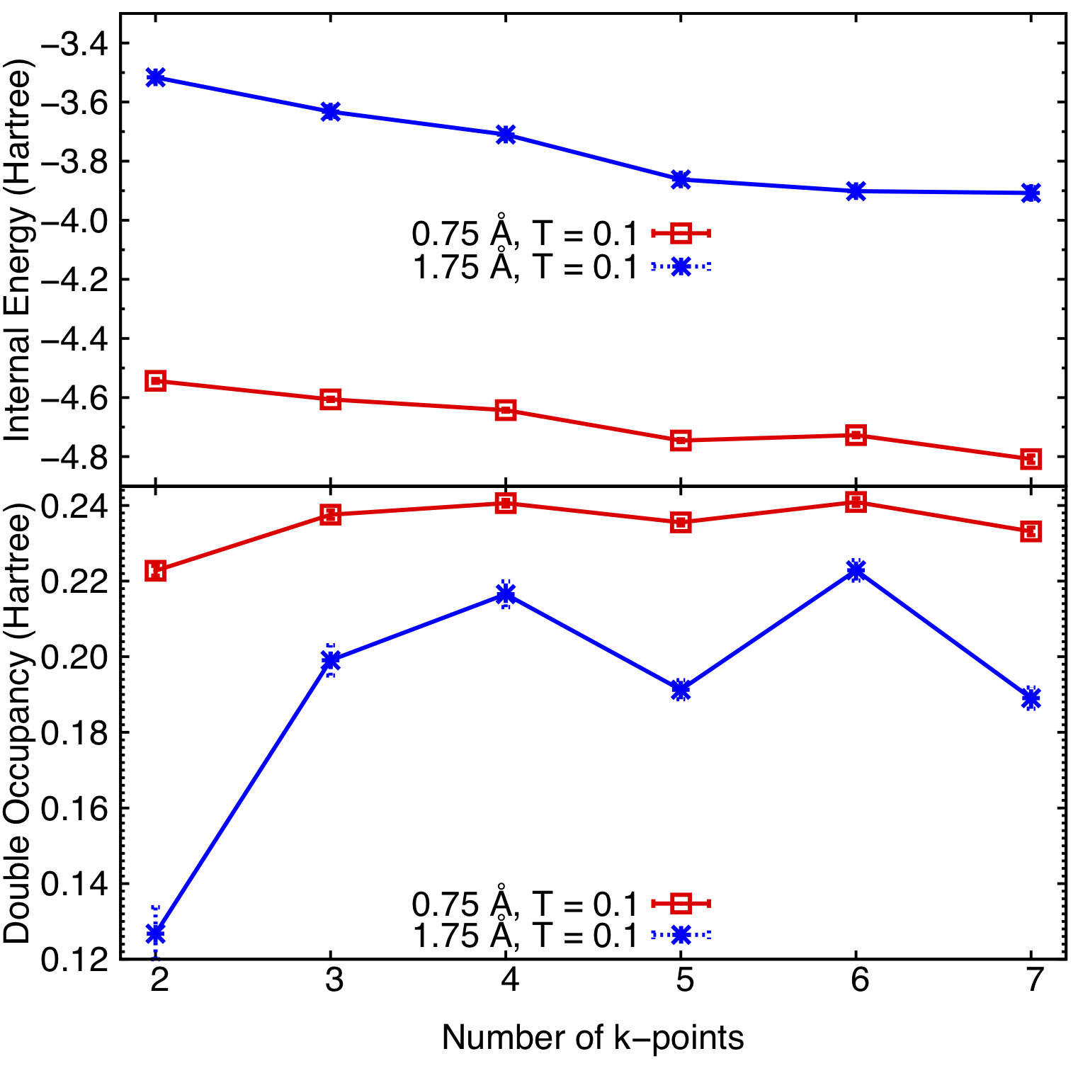
Figure 1: Internal energies (upper panel) and double occupancies (lower panel) of hydrogen chains at H-H bond lengths of 0.75 (red empty squares) and 1.75 (blue dot crosses) Å as a function of the number of k-points sampled in the first Brillouin zone. All of the results are calculated at a temperature of $T=0.1$ Hartree/$k_{B}$.

3.2 Effective Interaction Strengths and Temperatures of the Hydrogen Chains

In order to analyze our simulation results, it is insightful to first contextualize the effective interaction strengths of our hydrogen chains in terms of 1D Hubbard ⁶⁹ and extended Hubbard ⁷⁰ model effective interaction strengths. While hydrogen chains obviously possess long-range interactions that span their length and distinguish them from Hubbard models, to develop intuition, we investigate the magnitudes of their on-site and nearest-neighbor inter-site Coulomb repulsions, as well as their hopping matrix elements.

To do so, in Figure 2, we plot the inter-site (a) one-body hopping matrix elements, $T_{1\bm{\Gamma}\uparrow,i\bm{\Gamma}\uparrow}$ (denoted as $t_{1i}$ in the following) and (b) density-density Coulomb repulsions, $V_{1\bm{\Gamma},i\bm{\Gamma},1\bm{\Gamma},i\bm{\Gamma}}^{\uparrow\uparrow\uparrow\uparrow}$ (denoted as $U_{11ii}$), between atoms 1 and $i$ as a function of atom label $i$ at the $\bm{\Gamma}$ point for two up electrons. From the plot, it is evident that chains with shorter bond lengths have larger magnitude hopping matrix elements and Coulomb repulsions than chains with longer bond lengths, which is consistent with the larger overlap between $1s$ wave functions on more closely spaced hydrogen atoms. Nevertheless, while the magnitudes of the $t_{11}$ matrix elements appreciably change with bond distance, the $U_{1111}$ matrix elements remain roughly constant with bond length because they are largely determined by the shape of the on-site $1s$ wave function, which remains the same irrespective of bond length. Indeed, at a particular bond length, the inter-site hopping matrix elements decrease roughly exponentially as the distance between two atoms increases, while the inter-site Coulomb repulsions only decay as roughly $1/r$ where $r$ is the distance between two atoms. Note that the smallest magnitude interaction strengths appear between atoms 1 and 6 at the $\bm{\Gamma}$ point because all of the atoms beyond atom 6 are actually closer to atom 1 due to the periodic boundary conditions we imposed on our models.

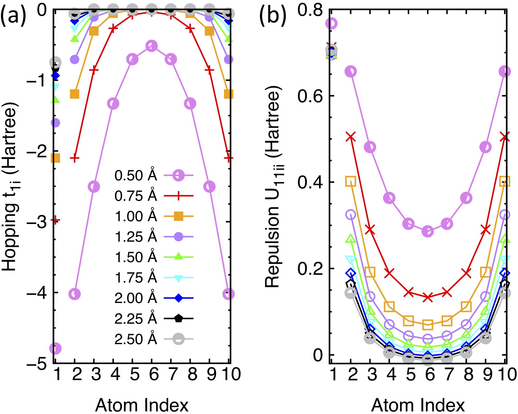
Figure 2: Interaction strengths of selected (a) one-body hopping terms, $t_{1i}$, and (b) two-body Coulomb repulsions, $U_{11ii}$, of hydrogen chains for different bond lengths. $t_{1i}$ denotes the hopping matrix element between sites 1 and $i$ at the $\bm{\Gamma}$ point, while $U_{11ii}$ represents the density-density Coulomb interaction between sites 1 and $i$ at the $\bm{\Gamma}$ point. Note that the diagonal terms, $t_{11}$ and $U_{1111}$, are purposefully plotted separately on the left.

Because the effective interaction strengths of our chains are more physically meaningful than their absolute interaction strengths, we calculate our chains’ effective interaction strengths, $U/t$, where $U$ is the Hubbard on-site repulsion and $t$ is the Hubbard hopping parameter, in the following way. First, the effective hopping, $t_{\text{eff}}$, may be defined as the magnitude of the nearest-neighbor hopping amplitude in the hydrogen chain, $t_{\text{eff}}=|t_{\langle i,j\rangle}|$. Second, since the on- and inter-site Coulomb repulsions scale differently with the bond length, we define two different effective Coulomb interaction strengths, $U_{\text{on}}$ and $U_{\text{inter}}$, where the former is taken as the on-site repulsion matrix element, $U_{1111}$, and the latter is obtained by fitting the decay of $U_{11ii}$ in Figure 2 to the form $U_{\text{inter}}/|1-i|$. The ratios of $U_{\text{on}}/t_{\text{eff}}$ and $U_{\text{inter}}/t_{\text{eff}}$ are finally evaluated and denoted as $\tilde{U}_{\text{on}}$ and $\tilde{U}_{\text{inter}}$, respectively. The resulting effective interactions are summarized in Table 1 for chains of different bond lengths.

$R_{H-H}$ (Å)	$t_{\text{eff}}$	$U_{\text{inter}}$	$\tilde{U}_{\text{inter}}$	$U_{\text{on}}$	$\tilde{U}_{\text{on}}$	$\tilde{T}_{\text{min}}$
0.50	4.79	0.47	0.10	0.77	0.16	0.01
0.75	2.10	0.47	0.23	0.71	0.34	0.02
1.00	1.20	0.43	0.36	0.70	0.58	0.04
1.25	0.71	0.37	0.52	0.69	0.98	0.07
1.50	0.43	0.32	0.74	0.69	1.62	0.12
1.75	0.26	0.28	1.06	0.70	2.67	0.19
2.00	0.16	0.25	1.54	0.70	4.38	0.31
2.25	0.10	0.22	2.24	0.70	7.18	0.51
2.50	0.06	0.20	3.32	0.71	11.78	0.83

Table 1: Interaction strengths of hydrogen chains with different bond lengths as quantified by the effective inter-site repulsion, $\tilde{U}_{\text{inter}}=U_{\text{inter}}/t_{\text{eff}}$, and on-site repulsion, $\tilde{U}_{\text{on}}=U_{\text{on}}/t_{\text{eff}}$. $t_{\text{eff}}$ is the nearest-neighbor hopping interaction from the original ab initio Hamiltonian. The effective temperature, $\tilde{T}_{\text{min}}=T_{\text{min}}/t_{\text{eff}}$, where $T_{\text{min}}=0.05$ Hartree/$k_{B}$, for each bond length is also listed in the last column.

Recall that the standard Hubbard model only accounts for on-site repulsion, so the $\tilde{U}_{\text{on}}$ given in Table 1 may serve as natural points of comparison between the Hubbard model and the chains studied here. Similarly, $\tilde{U}_{\text{inter}}$ plays the role of the nearest-neighbor interaction, $V$, in the extended Hubbard model. As can be observed from Table 1, the $t_{\text{eff}}$ decreases in magnitude with bond length, while $\tilde{U}_{\text{inter}}$, $\tilde{U}_{\text{on}}$, and $\tilde{T}_{min}$ all increase with bond length. That said, the shortest-length chains ($R\leq 1.25$ Å) essentially correspond to the 1D Hubbard model in the small $U/t$ regime ($U/t<1$). The 2.00 Å chain borders upon being strongly correlated (in one dimension) with a $U/t\approx 4$, while the $R\geq 2.25$ Å chains are very strongly correlated with $U/t\geq 7$. For all of the bond lengths studied, however, the inter-site interactions provided in the third and fourth columns of Table 1 maintain significant values not accounted for in the standard Hubbard model. Moreover, the strength of the inter-site repulsion relative to the on-site repulsion decreases as the bond length is increased. In particular, the $R=1.25$ Å chain marks a bond length beyond which $V/U$ dips below 0.5. This signifies that the longest-length chains more closely approximate the standard Hubbard model, while the shortest-length chains more closely approximate the extended Hubbard model. Since $\tilde{T}_{\text{min}}$ increases with bond length, this furthermore implies that the longest chains are effectively modeled at higher temperatures than the shortest chains. We will frequently return to these effective interactions and temperatures in the subsequent analysis of our chains’ physics.

3.3 Internal Energy Crossover

As an initial entry into the physics of our hydrogen chains, we first study how their internal energies vary as a function of temperature. We take $T=10$ Hartrees/$k_{B}$ as the upper temperature limit in our studies because 10 Hartrees/$k_{B}$ is larger than the effective $U/t$ for all but our 2.5 Å hydrogen chain. On the other hand, we take $T=0.05$ Hartrees/$k_{B}$ as the lower temperature limit in our studies because our hydrogen chains approach their ground state behavior at this temperature. Indeed, as depicted in Figure 3, at $T=0.05$ Hartrees/$k_{B}$, the internal energy according to both MFT and FT-AFQMC is lowest at a bond length of around 1.0 Å, which is comparable to the equilibrium ground state bond length of 0.945 Å found in previous work.^{40, 71}

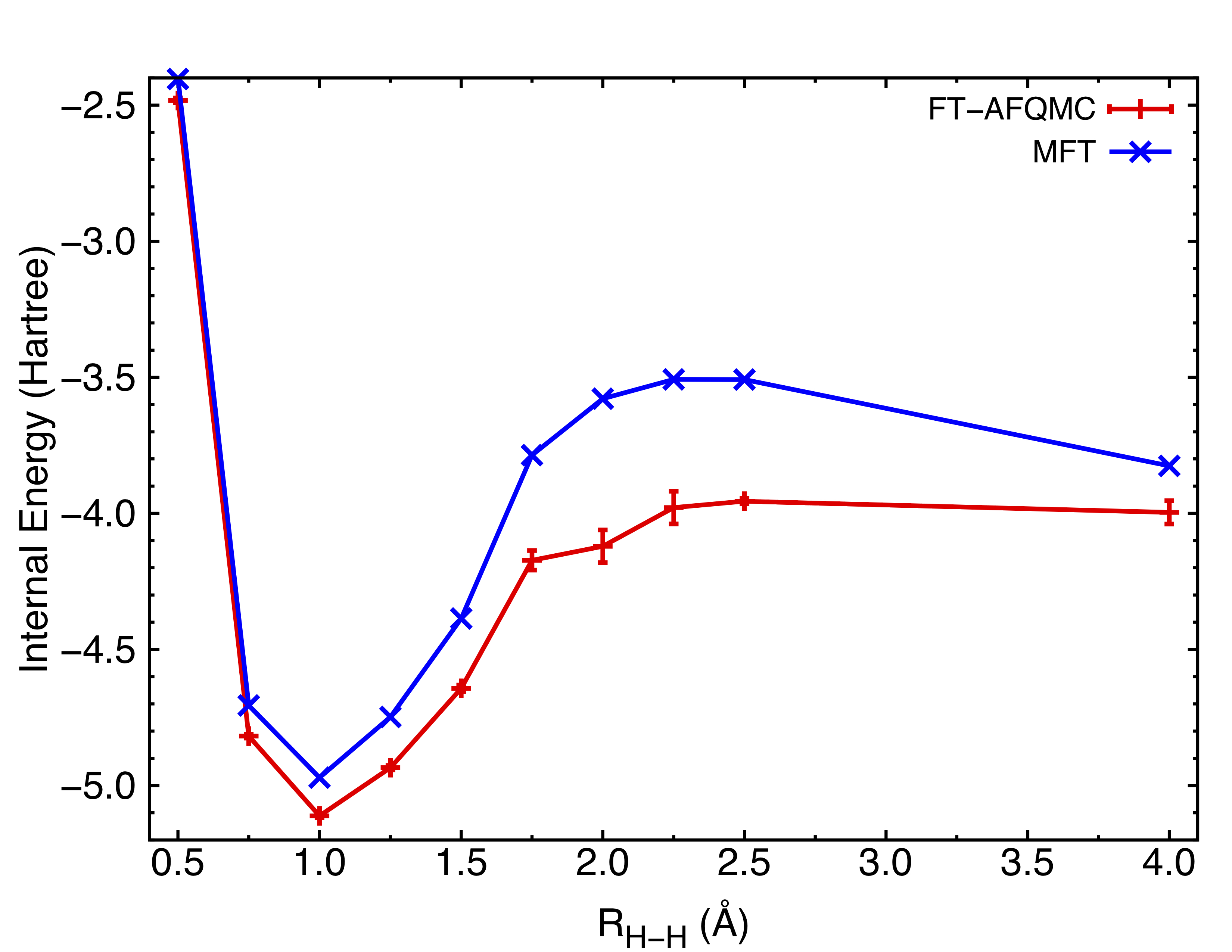
Figure 3: Internal energy of our hydrogen chains as a function of H-H bond length at $T=0.05$ Hartree/$k_{B}$, the lowest temperature employed in this study. The FT-AFQMC results are denoted by red $+$’s, while the MFT results are denoted by blue $\times$’s. The internal energy is minimized around 1.0 Å.

We moreover find that the FT-AFQMC energy at this near-equilibrium bond length approaches the 0.542 Hartrees/atom expected in the ground state.⁴⁰ Additionally notice that mean field theory predicts a false dissociation barrier around 2.0 Å which also appears in the Hartree-Fock dissociation curve of H₂ molecules.³⁶ In contrast, our many-body AFQMC results give the correct dissociative behavior. Thus, while modeling at $T=0.05$ Hartrees/$k_{B}$ is certainly not tantamount to modeling the ground state, our results suggest that this temperature is low enough to approximate many ground state features.

In Figure 4, we therefore turn to depicting how the internal energy varies for chains with differing bond lengths between these two limiting temperatures.

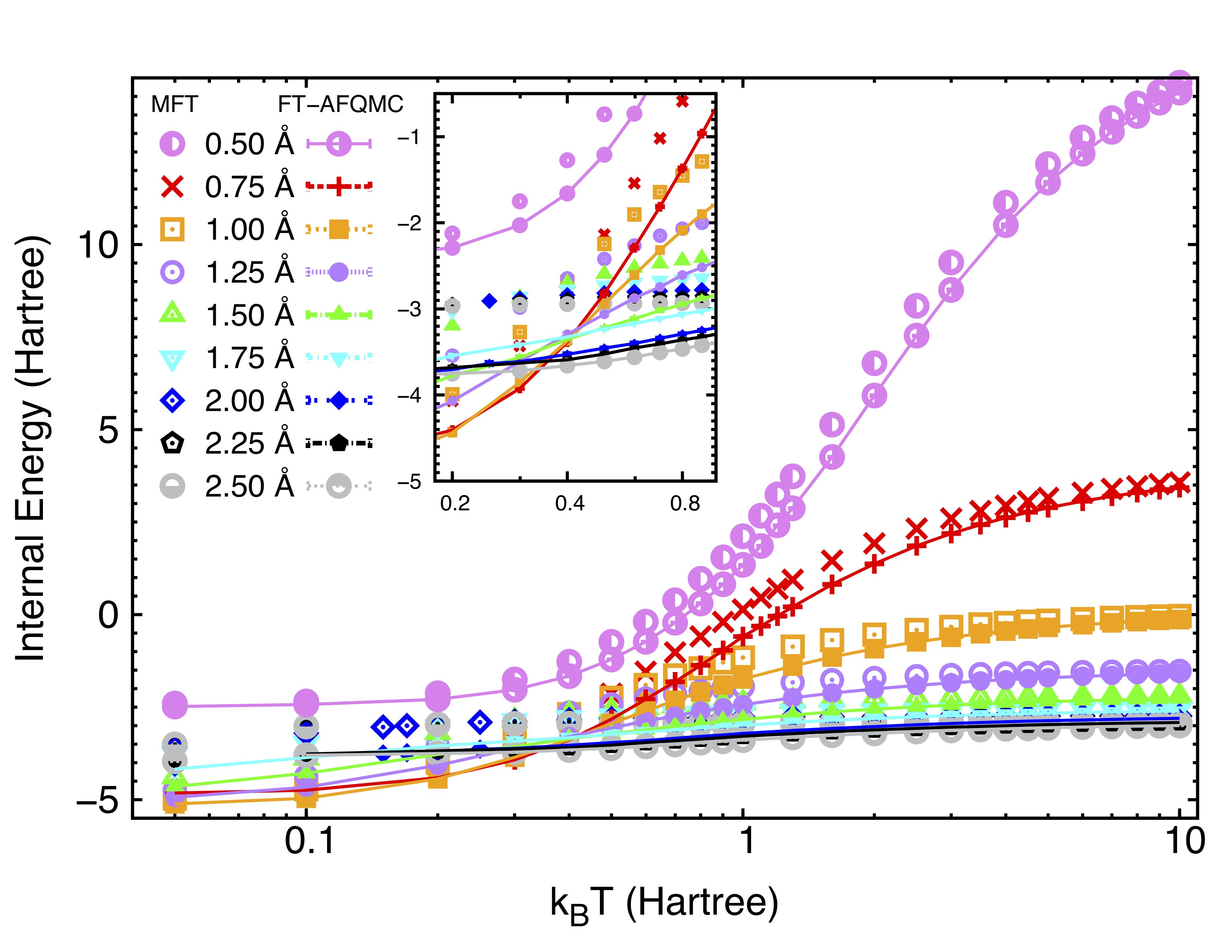
Figure 4: Internal energy of the hydrogen chains for different H-H bond lengths over a range of temperatures. The FT-AFQMC results are denoted by the solid symbols, which are interconnected by solid lines as a guide to the eye, while the MFT results are denoted by the open symbols. Different colors correspond to different bond lengths. Note that the horizontal axis is plotted on a log scale in order to emphasize the low-temperature behavior. The inset highlights the crossover regime at intermediate temperatures and is plotted on a linear scale.

As is clear from the figure, the 0.5 Å chain undergoes the largest change in internal energy of several Hartrees from low to high temperatures; this change monotonically decreases with increasing bond length, with the 2.5 Å chain manifesting a change of barely a Hartree. These differences between the energies of the low and high temperature states may be directly linked to the energy spread of the many-body eigenstates of the respective chains. As is well-known from the archetypal example of H₂ dissociation,³⁶ varying the bond length between atoms in a hydrogen chain varies the overlap among the hydrogens’ atomic wave functions, modulating their energy spread in turn. More specifically, when the H-H bond length is decreased, the highest energy state is pushed toward higher energies, while the lowest energy state is pushed toward lower energies, resulting in an overall increase in the energy spread – and vice-versa. By extension, the large change in internal energy with varying temperatures for the 0.5 Å chain is indicative of its states having a large energy spread, while the much smaller change for the 2.5 Å chain is indicative of its states being more concentrated in energy space (i.e., it has a larger density of states). Please see the Supplemental Information for a plot depicting the spread of the mean field states for all of the chains studied in this work for reference. Because of these varying distributions of states, a crossover is observed around a temperature of 0.4 Hartree/$k_{B}$, at which point the $R\geq 0.75$ Å chains reverse their energetic ordering. This is because the average energy for all of the chains is pushed upwards by the inclusion of the higher energy states that are accessed at high temperatures and these high energy states are even higher in energy for the small bond length chains. What is also clear from Figure 4 is that the mean field energies are universally greater than the many-body, FT-AFQMC energies. The correlation energy missed by mean field theory is generally expected to increase the attractive interactions among the atoms, leading to lower many-body energies, particularly at the intermediate temperatures (see the inset, Table LABEL:tab:mft-error, and Fig. LABEL:fig:eng-corr in the Supplemental Information for more details) at which previous work also found mean field discrepancies to be largest.³⁴

3.4 Heat Capacity Features

As discussed in Section 2.3.2, heat capacity curves provide more detailed signatures of the temperature dependence of different physical properties. To obtain the heat capacities, $C_{V}(T)$, we thus differentiate the internal energies provided in Figure 4 with respect to the temperature at a variety of bond lengths, as depicted in Figure 5. Since quantum Monte Carlo data possess intrinsic fluctuations, we attribute the small fluctuations in the heat capacity curves to numerical fluctuations introduced by the internal energy data and ignore them in our interpretations. This interpretation is supported by the fact that the largest fluctuations appear around exactly the temperatures which possess the largest statistical error bars (see Secs. LABEL:sec:cv-error and LABEL:ssec:cv-interp-compare of the Supplemental Information for a more thorough discussion of how these error bars were obtained and their consequences.)

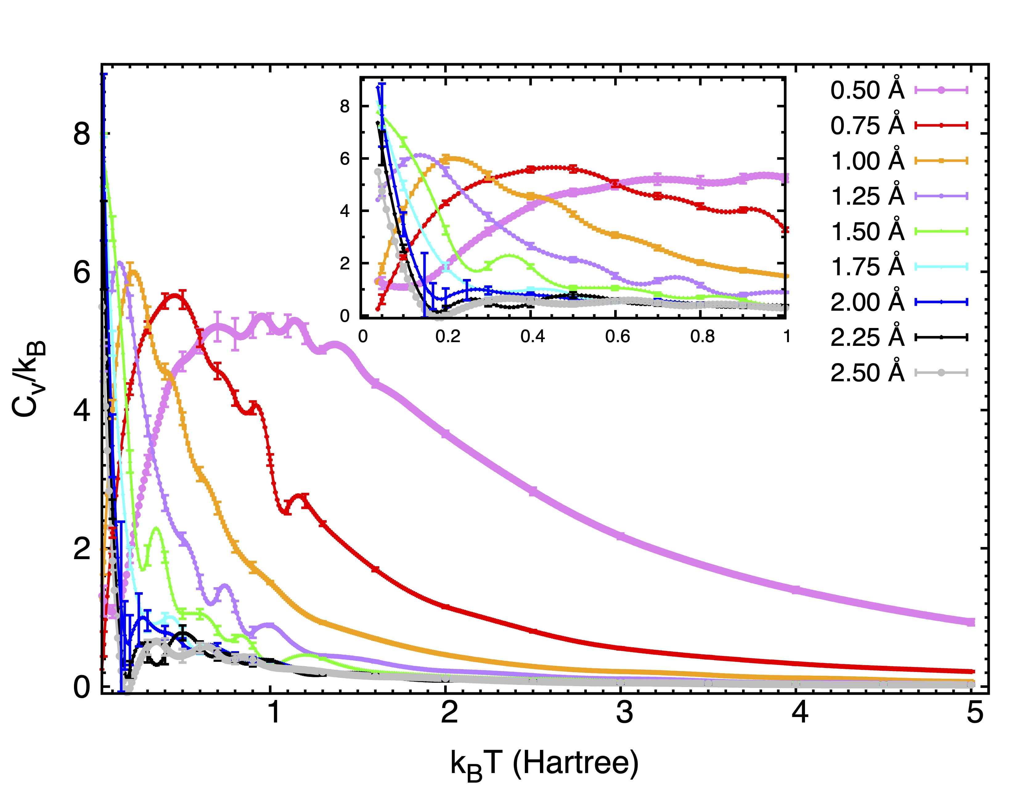
Figure 5: The heat capacity of the hydrogen chains at various bond lengths as a function of temperature. See Section 2.3.2 for more details on how the heat capacities were computed. The inset expands the low temperature regime from $T=0.05$ to 1 to ease identification of the most important heat capacity features. Note that the horizontal temperature axis is plotted on a linear scale. Error bars are depicted on the temperatures used in our interpolation.

For the $R=0.75$ Å chain, a single broad feature rapidly rises from zero at low temperatures, peaks around $T=0.5$, and then gradually decays to zero again in the high temperature limit. Similar peaks are also observed in the $R=0.5,1.0$ and $1.25$ Å chains, but as the bond length is increased (decreased), the corresponding heat capacity peak widths shrink (expand) while their heights increase (decrease), indicating a more rapid (gradual) response to temperature changes. For chains with bond lengths greater than 1.5 Å, the heat capacity peak is pushed to temperatures lower than those surveyed in this work. The fact that this peak shifts to lower temperatures with increasing bond lengths indicates that the excitation responsible for this peak requires less thermal energy to initiate at longer bond lengths.

We note that the results presented here generally agree with earlier numerical results obtained by Shiba ⁷² for the 1D Hubbard chain at finite temperature with a small number of sites in the grand canonical ensemble. However, there is one significant difference in the way our heat capacities vary with temperature. In the 1D Hubbard model, the heat capacity possesses a single broad feature in the small $U/t$ regime, but splits into two peaks for $U/t\geq 4$, where one of the two peaks lies between $0<T/t<0.5$ and is sharp, while the other lies in the high temperature regime between $0.5<T/t<5$ and is broad. According to Shiba, the sharp feature at low temperatures is due to a collective spin excitation from the antiferromagnetic ground state of the Hubbard model, while the broad peak in the high-temperature regime originates from a charge excitation across the Mott gap.

If our chains’ behavior is analogous to that seen in the Hubbard model, based upon their effective on-site interactions, we anticipate two peaks to be observed in the heat capacities of the 2.0, 2.25, and 2.50 Å chains. According to previous 1D Hubbard model results,⁷² we thus estimate the 2.00, 2.25, and 2.50 Å chains to have spin excitation peaks around 0.054, 0.022, and 0.0084 Hartree/$k_{B}$ and charge excitation peaks around 0.17, 0.14, and 0.15 Hartree/$k_{B}$ (see the Supplemental Information for further details regarding the Hubbard excitation temperatures). The expected spin excitation temperatures for the 2.25 and 2.5 Å chains thus fall below the temperatures simulated in the present work, but the spin excitation temperature for the 2.0 Å chain should be observable within our data. Nevertheless, we only observe one feature in the low temperature regime for the 2.0 Å chain. The expected high-temperature, broad feature is absent from our results for this chain, even though its effective U is greater than 4. Similarly, the high temperature peaks expected to occur around 0.14 and 0.15 Hartree/$k_{B}$ for the 2.25 and 2.5 Å chains also do not appear in our data. However, the decreasing width and increasing sharpness of the low-temperature peaks in our results agree with what Shiba observed of the low temperature peaks in the Hubbard model. It makes no sense to assume that the absence of the high-temperature feature in our simulations is due to the absence of charge excitations, because we know that, in the grand canonical ensemble, charge and spin excitations should both appear. As this comparatively simple model may only exhibit flavors of spin and charge ordering, this peak must be due to the emergence of either or both of these orders. So as to precisely characterize this order, we therefore proceed to analyze observables that are bellwethers of charge- and spin-related ordering in the following sections.

3.5 Trends in the Double Occupancy and a Metal-Insulator Crossover

In order to determine whether the heat capacity peaks stem from a form of charge ordering, we first examine the double occupancies of our hydrogen chains as a function of temperature. As discussed in Mott’s seminal paper, if the Coulomb repulsion among electrons in a material is stronger than the electrons’ propensity to hop among atoms, periodic lattices will manifest Mott insulating behavior in which charges remain localized even though they should delocalize according to conventional band theory.⁷³ Since the Coulomb repulsion among electrons in hydrogen chains can greatly exceed their propensity to hop at sufficiently long H-H bond lengths (see Section 3.2 for a more explicit discussion), Mott was thus able to show that 3D hydrogen lattices undergo a discontinous metal-Mott-insulator transition at bond lengths around 1.3 Å. Similar results were obtained using extended DMFT for two-dimensional systems.⁷⁴ We therefore anticipate a Mott insulator to emerge with increasing H-H bond distances in the 1D hydrogen chains studied here.⁷⁵ A simple gauge of the emergence of insulating behavior is the double occupancy, which measures the fraction of, in this case, atoms, that are occupied by two electrons.^{76, 77} Smaller double occupancies are indicative of correlated Mott insulating behavior in which strong electron-electron interactions suppress two electrons from occupying the same orbital (in this case, H, since each atom possesses only a single GTO), while larger double occupancies are indicative of less correlated, more metallic behavior in which electrons are free to occupy virtually any atom.

As depicted in Figure 6, we therefore calculated the average double occupancy per atom for our chains as a function of temperature using both FT-AFQMC (Figure 6a) and MFT (Figure 6b). We find that almost irrespective of the temperature, the double occupancy at shorter bond lengths is greater than that at longer bond lengths, which implies that our chains at shorter bond lengths are more metallic than those with longer bond lengths. In the high temperature limit ($T=10$), all electronic states are equally populated, implying that these hot electrons essentially exhibit classical behavior. As a result, electrons are as likely to inhabit an already occupied atom as an unoccupied atom. At half-filling, this signifies that half of the atoms will be randomly populated by up electrons and half will be randomly populated by down electrons, meaning that, as calculated, a quarter (0.25) of all atoms will be doubly occupied.

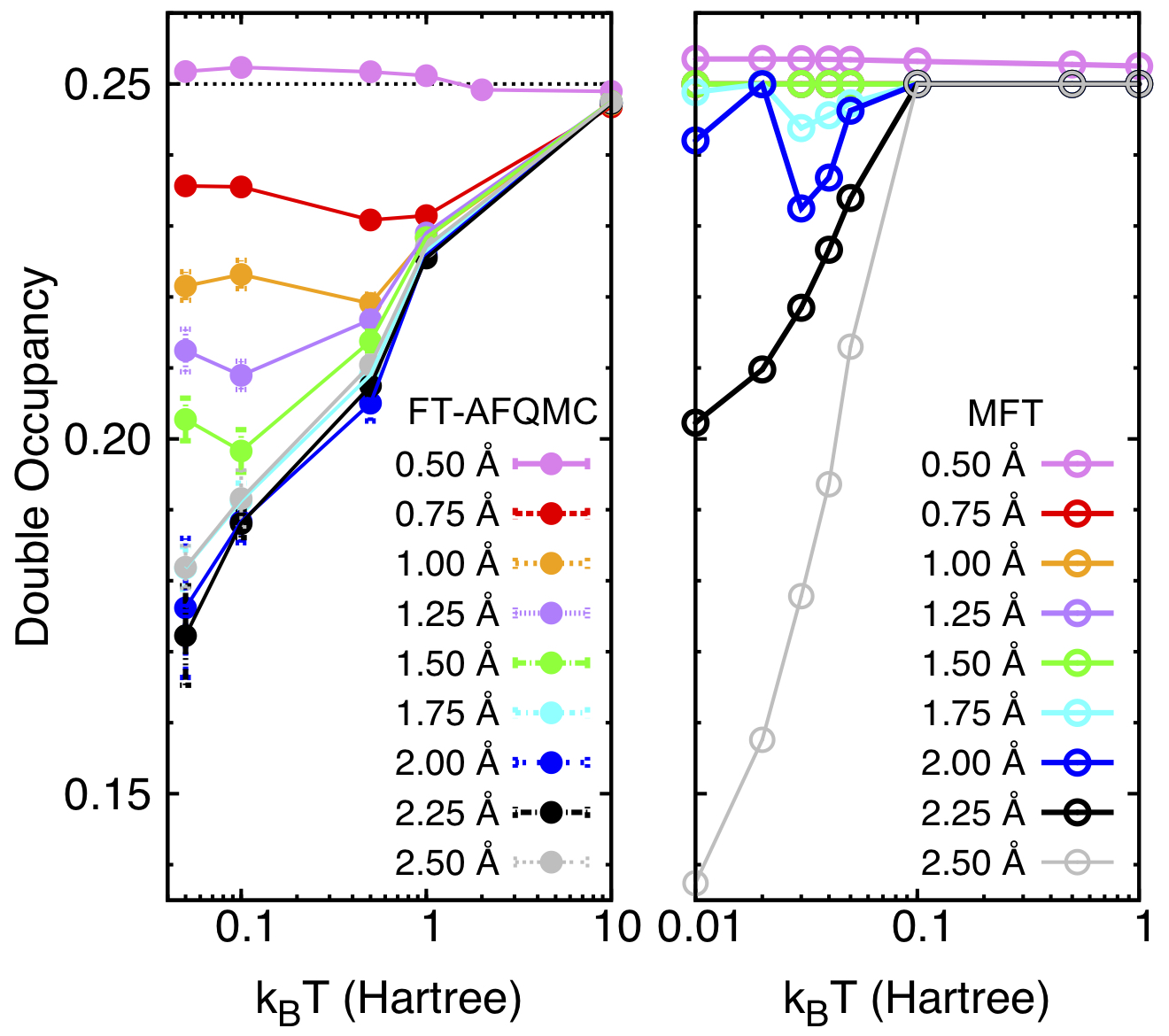
Figure 6: Double occupancy per atom of the hydrogen chains at different bond lengths over a range of temperatures according to (left) FT-AFQMC and (right) MFT. Different colors represent different bond lengths. Note that the ranges of the horizontal axes (in log scale) differ between the left and right panels.

In contrast, in the low-temperature limit, different chains manifest different metal-insulating behavior as a function of $R$. At the shortest bond length, $R=0.5$ Å, the double occupancy rises above 0.25 when the temperature is lowered, suggesting that the ground state of the $R=0.5$ Å chain is metallic. In contrast, when $R\geq 0.75$ Å, the double occupancy is suppressed as the temperature is lowered due to the increased Coulomb repulsion between electrons, which favors the formation of local moments. The fact that the double occupancy increases for the 0.5 Å chain, yet decreases for the 0.75 Å chain is consistent with recent work on ground state hydrogen chains which predicts a first order metal-insulator transition to occur around a bond length of roughly 1.5 Bohr = 0.794 Å.³⁹

Interestingly, for $0.75$ Å $\leq R\leq 1.5$ Å, a minimum in the double occupancy may be observed to occur between 0.1 and 1 Hartree/$k_{B}$. The somewhat counterintuitive negative-sloping double occupancy curve that emerges at low temperatures stems from an effect analogous to the Pomeranchuk effect in the Hubbard model:^{78, 79, 80} as the temperature is increased through the low temperature regime, the formation of local spin moments (indicated by decreasing double occupancies) will increase the entropy of the spin degrees of freedom, thus decreasing the free energy and stabilizing the system. To the best of our knowledge, this is the first observation of such a phenomenon in the presence of long-range Coulomb interactions. As $R$ is further increased beyond 1.75 Å, the effects of strong correlation dominate over the entire temperature range explored, resulting in only positive-sloping double occupancies, which further corroborate Mott-insulating behavior.

We furthermore note that MFT fairly accurately predicts the double occupancy at high temperatures, but significantly overestimates it (thus also overestimating the metallic character of the chains) at low temperatures, particularly for strongly correlated chains with $1.50\leq R\leq 2.25$ Å. This is consistent with the well-known fact that mean field theories, such as Density Functional Theory, often wrongly predict metallic behavior for strongly correlated insulators such as NiO.^{81, 82}

Lastly, it is illuminating to plot the double occupancy as a function of $R$ at low temperatures, as shown in Figure 7. As discussed above, we can clearly see a crossover from metallic to insulating behavior between $R=0.5$ and $R=0.75$ Å. Comparing the left and right panels of Figure 7, it is also evident that FT-AFQMC captures the effects of correlation irrespective of the bond length, while MFT seems to be ignorant to the increasing degree of correlation up until $R=1.75$ Å, after which it predicts a sharp drop in the double occupancy at temperatures lower than 0.05 Hartree/$k_{B}$. For temperatures greater than that, MFT predicts a double occupancy of 0.25, which is the same as that expected in the high temperature limit. The sudden drop in the double occupancy at low temperatures in the right panel suggests that MFT predicts a finite temperature crossover into the Mott insulator regime at around $R=1.75$ Å.

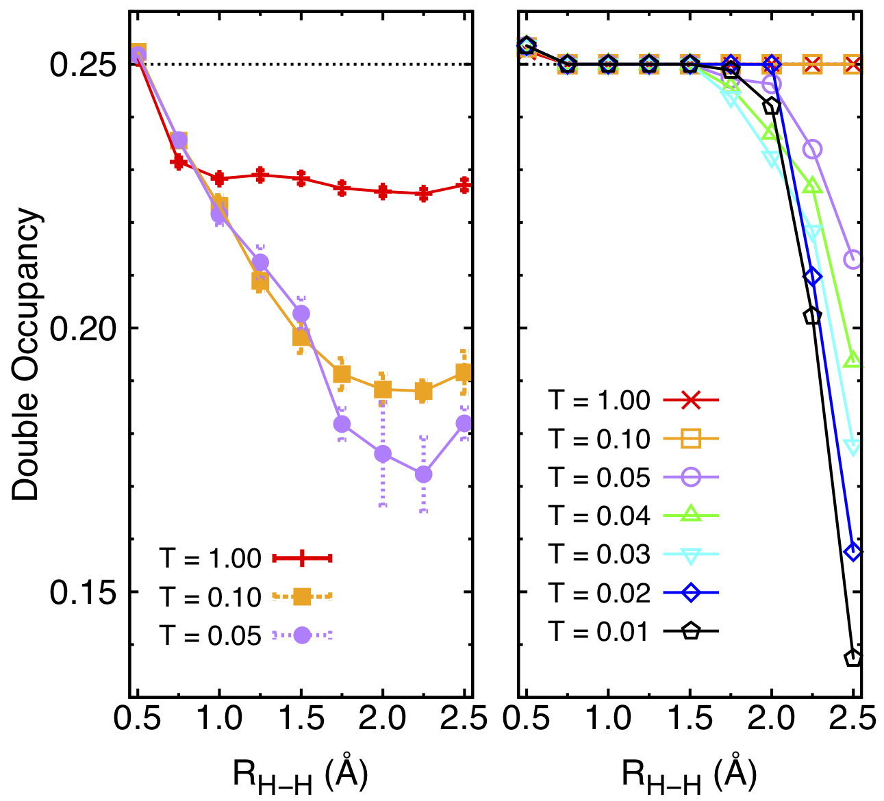
Figure 7: Double occupancy per atom of the hydrogen chains as a function of bond length for several temperatures according to (left) FT-AFQMC and (right) MFT calculations. Different colors represent different temperatures.

3.6 Magnetic and Insulating Crossovers as Revealed by Spin-Spin and Charge-Charge Correlation Functions

In order to characterize the spin and charge excitation contributions to the heat capacity of our hydrogen chains, we compute spin-spin, $C_{ss}$, and charge-charge, $C_{cc}$, correlation functions for all chains at $T=1.0$, 0.1, and 0.05 Hartree/$k_{B}$, as shown in Figures 8 and 9, respectively.

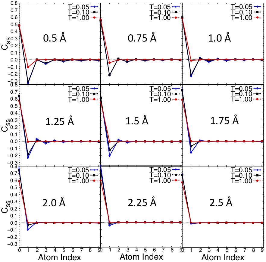
Figure 8: The spin-spin correlation functions, $C_{ss}$, of the hydrogen chains at different bond lengths and temperatures ($T=$ 0.05, 0.1, and 1 Hartree/$k_{B}$) calculated using FT-AFQMC. The horizontal dashed line in each panel at $C_{ss}=0$ is a guide to the eye.

As described in Section 2.3.5, all of the correlation functions presented were computed in the orthogonal atomic orbital basis. The positivity of the correlation functions at site 0 is guaranteed since charges and spins should be most correlated with themselves, while the large dips in all of the charge-charge and spin-spin correlation functions at site 1 are a direct consequence of correlation and exchange holes, respectively. In Figure 8, at $T=0.05$, AFM order clearly emerges for chains at bond lengths of 0.75, 1.0, 1.25, and 1.5 Å, as can be seen from the alternating positive and negative values of $C_{ss}$. For $R=0.5$ Å, however, the correlation functions remain negative for all atoms greater than 1. This is indicative of ferromagnetic (FM) ordering. The sign change of the correlation functions from $R=0.5$ to 0.75 Å suggests a crossover from FM order to AFM order at low, but finite temperatures. For chains with longer bond lengths ($\geq 1.75$ Å), AFM order dissipates at the temperatures explored because of their smaller effective exchange coupling strengths. At still longer bond lengths ($\geq 2.25$ Å), even the exchange hole is barely visible, indicating the vanishing effective exchange at these temperatures. Note that the correlation functions do not exhibit the same periodicity as seen in Fig. 2 because our hydrogen chain results have been averaged over 5 k-points (not just the $\Gamma$ point), which would be equivalent to performing simulations on a supercell of 50 hydrogen atoms at the $\Gamma$ point.

The charge-charge correlation functions also exhibit oscillations between positive and negative values at low temperatures for $R\leq 1.25$ Å. This is indicative of charge ordering, but over a slightly smaller range of bond distances than AFM or FM order is observed in the $C_{ss}$. The emergence of charge order for the shorter bond length chains is likely due to their larger ratio of nearest-neighbor to on-site Coulomb repulsion, as discussed in Section 3.2. Indeed, previous work ^{47, 83, 49} on the extended Hubbard model predicts the formation of a charge density wave (CDW) phase when $U$ and $V$ satisfy $V/U>c$, where $c$ is roughly 0.5, and a spin density wave (SDW) phase for $V/U$ smaller than that. Table 1 clearly suggests that for $R\leq 1.25$ Å, the effective inter- and on-site repulsion strengths, $\tilde{U}_{\text{inter}}$ and $\tilde{U}_{\text{on}}$, satisfy the criteria for favoring CDW formation. Chains with $R\geq 1.5$ Å exhibit no significant charge order except for their correlation holes. Note that the error bars on these charge-charge correlation functions are larger than those on our spin-spin correlation functions because the charge-charge correlation functions involve subtracting off background terms that possess their own error bars. The lowest temperature charge-charge correlation functions possess the largest error bars because they are most strongly correlated.

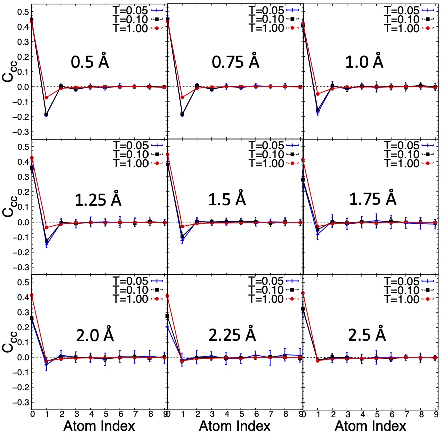
Figure 9: The charge-charge correlation function, $C_{cc}$, of the hydrogen chains at different bond lengths and temperatures ($T=$ 0.05, 0.1, and 1 Hartree/$k_{B}$) calculated using FT-AFQMC. The horizontal dashed line in each panel at $C_{cc}=0$ is a guide to the eye.

Combining this information with our previous observations about the double occupancies, our results suggest that the 0.5 Å chain will be a ferromagnetic metal, while the 0.75 Å chain will be an antiferromagnetic insulator in the ground state, as was observed in recent zero temperature studies.³⁹ In this work, we did not model chains with bond lengths shorter than 0.5 Å, but it would be interesting to examine the remnants of this ground state quantum phase transition at temperatures slightly above zero, at which both quantum and thermal fluctuations can play important roles. We leave this to future explorations. Our simulations thus reveal two metal to insulator crossovers: a ground state quantum phase transition that occurs upon varying bond length, and as described in Section 2.3.4, a finite temperature crossover that may be observed in all chains with $R\geq 0.75$ Å.

Our correlation functions also reveal an interesting interplay between the spin and charge degrees of freedom in hydrogen chains. Firstly, the existence of both spin and charge orders at low temperatures and the absence of both orders at higher temperatures indicates that the spin and charge degrees of freedom are coupled together in hydrogen chains. Unlike in the 1D Hubbard model, spin and charge excitations do not separately appear at different temperatures. Secondly, note that the value of $C_{ss}$ at site 0 (which measures the autocorrelation between an atom and itself) in Figure 8 increases from around $C_{ss}=0.5$ at $R=0.5$ Å to 0.8 at $R=2.5$ Å at low temperatures, while $C_{cc}$ in Figure 9 displays the opposite trend. The increasing local spin moment, yet decreasing charge-charge repulsion on a single atom corroborates the gradual development of stronger and stronger AFM order as $R$ is increased. Indeed, in a perfect AFM phase, $C_{ss}$ and $C_{cc}$ on atom 0 should assume a value of 1 and 0 respectively, since there should only be one electron occupying each atom and spins on adjacent atoms should anti-align. The coupling of spin and charge degrees of freedom is most likely mediated by the long-range Coulomb interactions inherent to such realistic systems.

3.7 Natural Occupancies in the Orthogonal AO Basis

To obtain further support for the ordering assignments we make above, we additionally computed the chains’ natural occupancies and orbitals by diagonalizing their density matrices in the orthogonal, periodic AO basis (see the Supplemental Information for more information about this basis and process).⁸⁴ In Figure 10, we plot the natural occupancies of all of the orbitals of all of our chains at the lowest temperature in our simulation, $T$ = 0.05 Hartree/$k_{B}$.

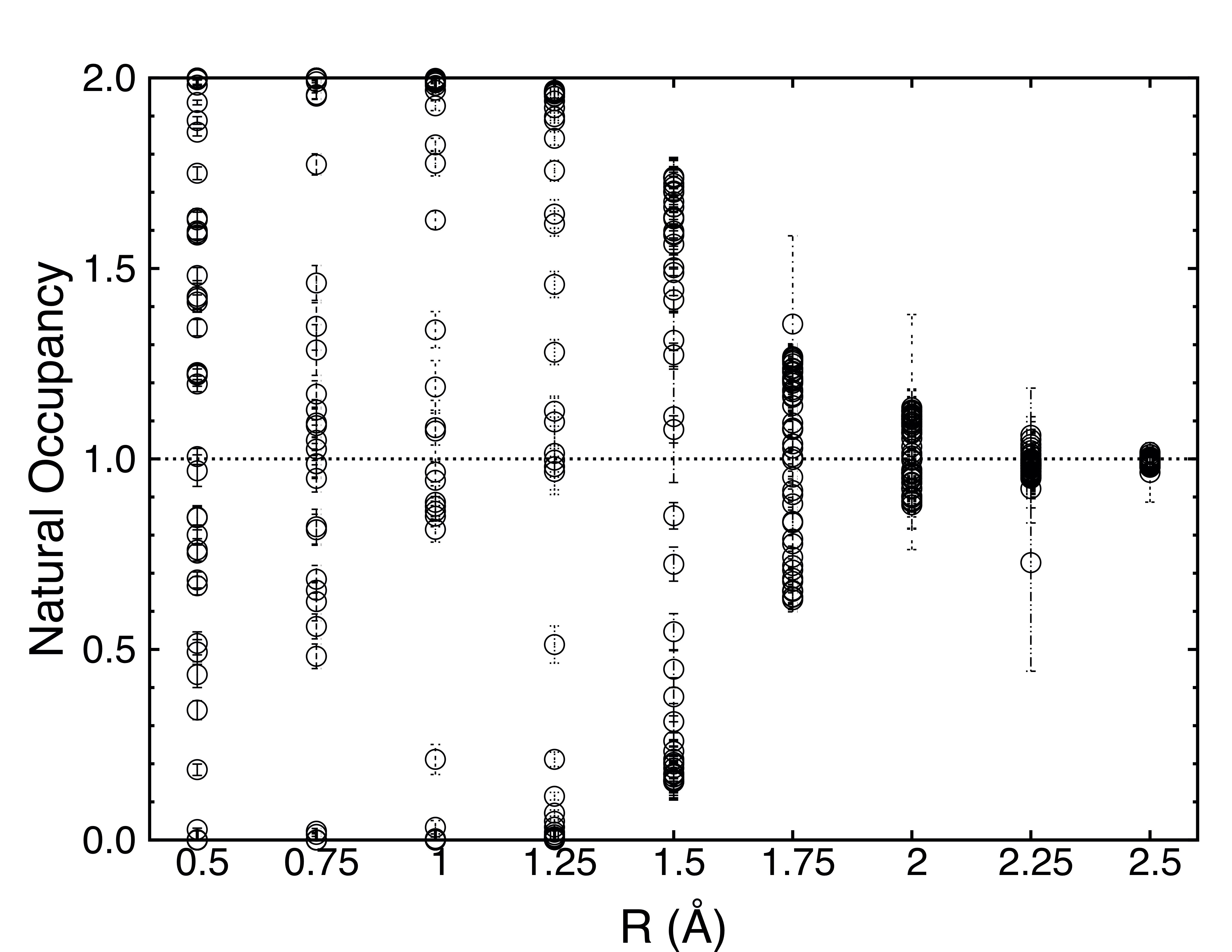
Figure 10: Natural occupancies of the natural orbitals of the hydrogen chains for all bond lengths studied at $T$ = 0.05 Hartree/$k_{B}$. 50 natural occupancies, which stem from the 50 p-GTOs employed in these simulations, are plotted for each bond length. The natural occupancies are obtained by diagonalizing the density matrix expressed in terms of the orthogonal, periodic AO basis.

For $R=0.5$ Å, we see that the natural occupancies are scattered across a wide range of values, many of which are fractional, corroborating that the chain is metallic. As the bond length is increased to 0.75, 1.0, and 1.25 Å, the natural occupancy tends to concentrate in empty, singly-occupied, and doubly-occupied natural orbitals, with little in between. As the chains are further stretched to 1.5 Å, the double occupancy (and, accordingly, zero occupancy) is further suppressed and the natural occupancies further concentrate around one, marking the onset of Mottness. Indeed, at 2.5 Å, all natural orbitals are singly occupied, which is indicative of a perfect Mott insulator.

The qualitative change of the distribution of natural occupancies from the 0.5 Å chain to the 0.75 Å chain, choruses with the metal to insulator crossover manifested in Figure 7, and the disappearance of the natural occupancy cluster around one from the 1.25 Å chain to the 1.5 Å chain coincides with the disappearance of charge order in Figure 9. We further note that, although the natural occupancies presented here are calculated at a low temperature of $T=0.05$ Hartree$/k_{B}$, contributions from thermal excitations may still exist, especially for chains with longer bond lengths and correspondingly larger effective temperatures.

At a given bond length, we can imagine that by varying the temperature, electrons can be thermally excited to higher lying bands which can change the occupancy of the chain. To further investigate such temperature effects, we plot the natural occupancies for the 1.0 Å chain as a function of temperature in Figure 11.

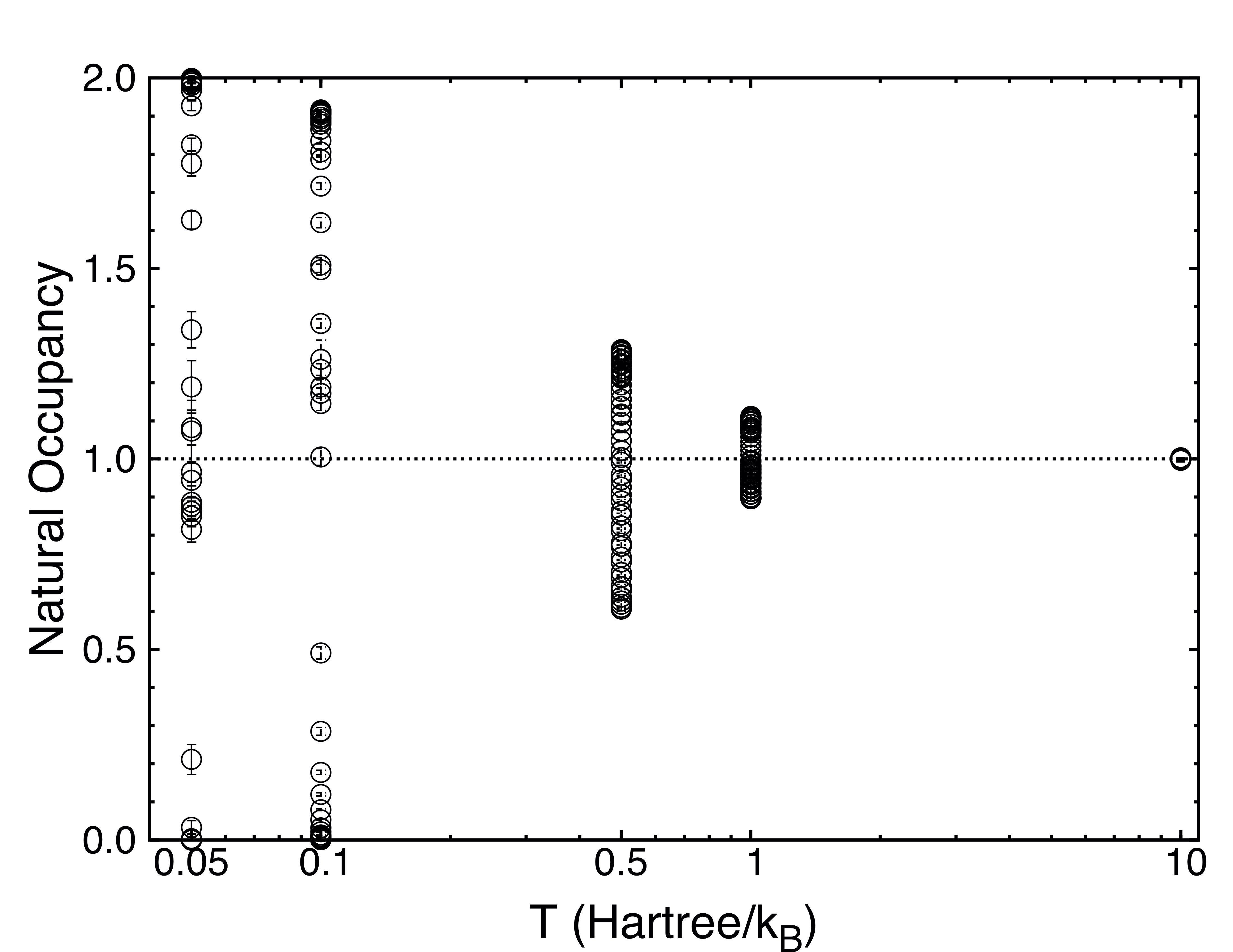
Figure 11: Natural occupancies of the 1.0 Å chain at $T=$ 0.05, 0.1, 0.5, 1, and 10 Hartree/$k_{B}$ in the orthogonal, periodic AO basis.

From this plot, we can observe that, as the temperature is increased, the spread of the natural occupancies tends to decrease and the natural occupancies all concentrate around one. This is because, as the temperature is increased, the kinetic energy of the electrons increases, making it easier for electrons that previously inhabited empty and doubly-occupied natural orbitals to instead inhabit singly-occupied natural orbitals. Note that the reason for the suppression of empty and double occupancy at high temperatures in Figure 11 differs from that for Figure 10 in long bond length chains, as the latter is due to Mottness induced by strong on-site Coulomb repulsions. The two scenarios can be easily distinguished by their completely different double occupancies as shown in Figure 7.

3.8 The Grand Potential and Entropy

Ultimately, finite temperature phase transitions are dictated by changes to a system’s free energy, in this case, the grand potential. Unfortunately, the Mermin-Wagner Theorem dictates that thermal fluctuations at even infinitesimally small, yet non-zero temperatures will break any long-range order within one-dimensional systems,^{85, 86} so finite temperature phase transitions cannot rigorously occur in the chains modeled here. Even at zero temperature, only quasi-long-range (instead of truly long-range) AFM order was observed in hydrogen chains.³⁹ Therefore, in this Section, we present the grand potentials and entropies of our chains in Figure 12 followed by only a very brief discussion of their physical significance.

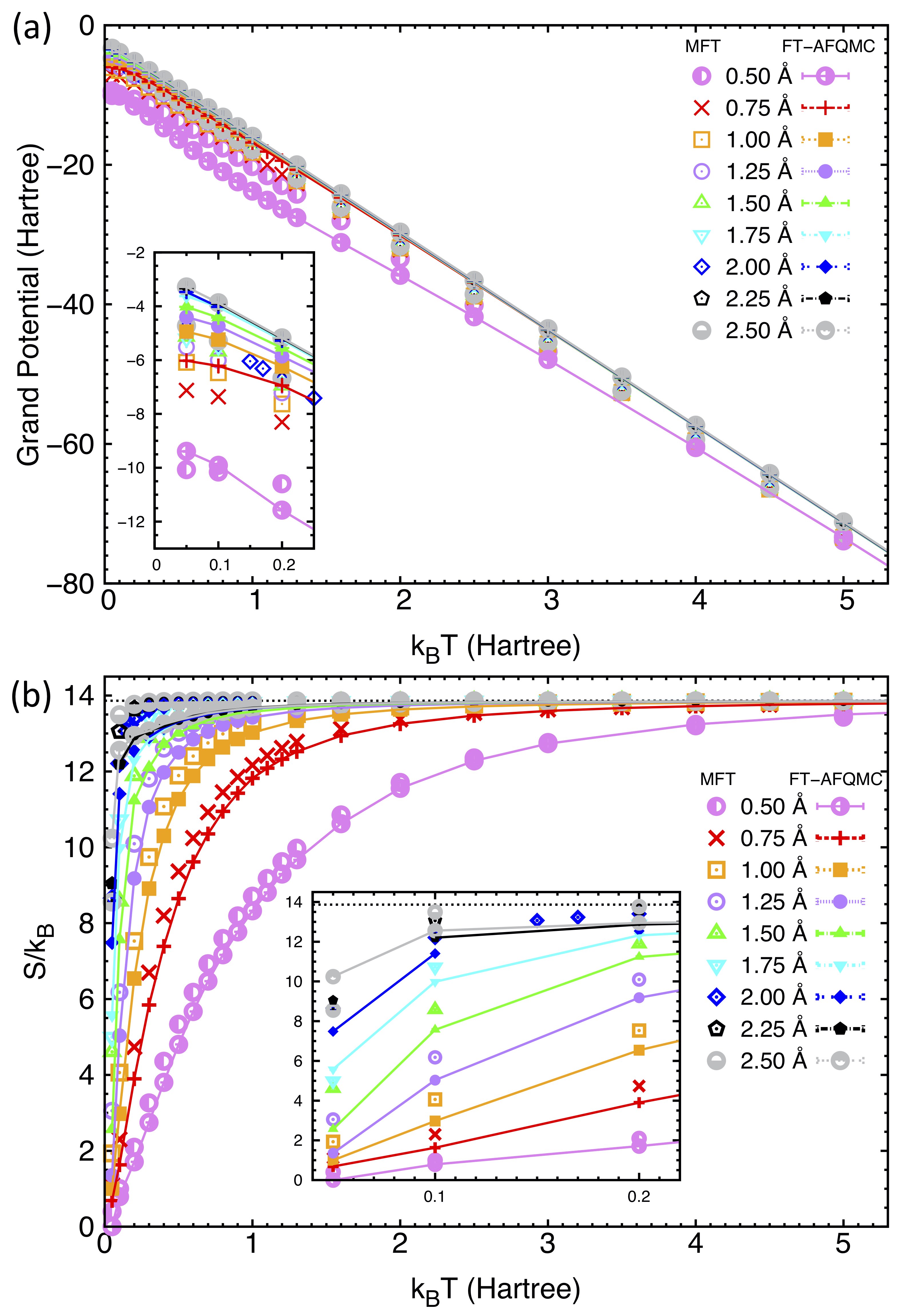
Figure 12: The grand potential (a) and entropy (b) of hydrogen chains at different bond lengths calculated using both FT-AFQMC and MFT. The horizontal black dashed line in (b) is the high temperature limit of the exact entropy for a ten-orbital system, which is $10ln4$.

As presented in panel (a) of Figure 12, at high temperatures, the grand potential depends linearly on the temperature, consistent with Equation (19), since in the high-temperature limit, all states are equally populated and the grand canonical partition function is constant. The grand potential remains linear at intermediate temperatures, illustrating the importance of the entropic, $-TS$ contribution to the partition function. At the low temperatures magnified in the inset, we observe that the grand potential plateaus for the 0.5 and 0.75 Å chains. This plateau is delayed to even lower temperatures not presented here for chains with longer bond lengths and hence larger effective temperatures. From panel (b), it is clear that the entropy for all chains in the high temperature limit assumes a value of $10ln4$, which is the theoretical high temperature limit of the entropy for a system with 10 spatial orbitals (and 4 potential electronic states per orbital) in the grand canonical ensemble. As the temperature is lowered, the entropy of all chains starts to decrease at different characteristic temperatures roughly determined by the chains’ band widths. In the low temperature limit, the entropy of all chains tends to converge to zero, as can be seen from the inset of panel (b). For the chains with bond lengths of 0.5, 0.75, 1.0, and 1.25 Å, for $T<0.2$, we observe that the entropy scales linearly with temperature and extrapolates to zero at zero temperature. The same linear behavior is likely to be observed in the longer bond length chains at temperatures below $T=0.05$ because they possess larger effective temperatures. Compared with the AFQMC results, MFT systematically underestimates the grand potential and overestimates the entropy.

We should also note that, from Figure 12, the grand potentials and entropies of chains with shorter bond lengths are consistently smaller than those with longer bond lengths irrespective of the temperature. The entropy is smallest for shorter chains because these chains possess larger band widths, meaning that fewer of their states will be accessible at any single temperature. As is also presented in Table 1, shorter bond length chains possess lower effective temperatures than longer bond length chains at the same physical temperatures. The ordering of the grand potentials may be explained by the magnitudes of their chemical potential terms, $-\mu N$. Shorter bond length hydrogen chains possess larger average electron densities. Larger electron densities lead to larger Coulomb repulsions among electrons, which means that larger magnitude chemical potentials are required to maintain a fixed average number of electrons. As a result, the larger negative contribution from the chemical potential term drives down the grand potential for shorter bond length chains.

4 Conclusions

In conclusion, we have generalized our previous fully ab initio finite temperature Auxiliary Field Quantum Monte Carlo method to solids and employed it to study the many-body thermodynamics of periodic hydrogen chains. Despite being the simplest possible models of ab initio solids in principle, hydrogen chains manifest an elaborate array of interrelated metal-insulator and magnetic orders, making them a meaningful testbed for studying the phase behavior of more complex solids. By calculating these chains’ many-body internal energies, free energies, entropies, double and natural occupancies, spin and charge correlation functions, and heat capacities as a function of H-H bond length and temperature, we demonstrated that, at low temperatures, they undergo metal to insulator and ferromagnetic to antiferromagnetic crossovers at bond lengths between 0.5 and 0.75 Å. Charge ordering is shown to emerge in chains with bond lengths less than or equal to 1.25 Å and a Mott insulating phase is predicted for bond lengths greater than 1.5 Å. Upon increasing the temperature beyond 1 Hartree/k_B, we observe the emergence of metallic character and the decay of any accompanying magnetic order in all of the chains studied. At intermediate bond lengths, we moreover see signatures of a Pomeranchuk effect in both our AFQMC and MFT results, the first time this has been identified in a realistic one-dimensional solid. In contrast with the heat capacity curves of one-dimensional Hubbard chains which exhibit two peaks for sufficiently large $U$ values, we find that the heat capacity curves of the chains analyzed here possess just a single peak, which we attribute to their distinctive coupling of spin and charge degrees of freedom. Such results highlight the important role long-range Coulomb interactions – and techniques capable of treating them – assume in determining the phase diagrams of realistic solids.

As this study has served as an initial foray into the finite temperature physics of hydrogen chains, several key aspects of our modeling can be improved in follow-up work. First and foremost, for computational expediency and to facilitate comparisons with the single-band Hubbard model, we employed a minimal STO-6G GTO basis set with limited k-point sampling, meaning that we have not fully converged our calculations to the thermodynamic limit. Increasing the size of our GTO basis will predominantly help converge localized states, while increasing our k-point sampling will help converge delocalized states and alleviate finite size effects. As discussed in the Supplemental Information, the path to converging to the thermodynamic limit at finite temperatures, however, is less well-paved than for the ground state. This is because finite temperature calculations inherently involve contributions from high-lying electronic states that converge to the thermodynamic limit differently than the ground state and often require significantly large bases. Indeed, the form of the finite size scaling for the uniform electron gas has been found to be temperature-dependent. ^{87, 63, 28} Achieving the thermodynamic limit for solids in the ground state is most often accomplished by adding both one- and two-body finite size corrections to finite size energy calculations.^{88, 89} Recently, accurate finite size corrections for the uniform electron gas at finite temperatures were derived by combining quantum Monte Carlo simulation results with corrections obtained from random-phase or Singwi-Tosi-Land-Sjölander approximations at small momentum $k$. ^{90, 91} Analogous finite temperature corrections for ab initio solids have yet to be methodically developed, making rigorous convergence to the thermodynamic limit beyond the scope of this work. Upon including finite size corrections, it may turn out that additional features may emerge in our heat capacity and other curves. This would be a useful point for future works to resolve. We therefore encourage future community efforts aimed at deriving such corrections.

Convergence challenges aside, our work brings into focus a number of other algorithmic improvements that will need to be developed to map the finite temperature phase diagrams of more complex, ab initio solids. Lacking better, less costly ways of estimating many-body thermodynamic quantities, in this work, we chose to compute entropies and free energies based upon internal energy data. Nevertheless, the many-body entropy can be directly obtained by taking the logarithm of the many-body density matrix, which requires expanding the logarithm into an infinite number of terms involving increasingly higher powers of the density matrix.⁶⁴ Future thought should therefore be devoted to deriving more computationally accessible estimators of thermodynamic quantities for ab initio treatments that would enable the more accurate characterization of phase diagrams and provide a means of independently validating estimates based upon the energy alone. Moreover, in this work, we simulated down to effective temperatures of 0.01 for the 0.5 Å chain and 0.83 for the 2.50 Å chain (see the last column of Table 1), which precluded us from observing the spin excitations one would expect to observe at even lower temperatures for chains with $R>2.25$ Å  based upon Hubbard model simulations.⁷² To study temperatures immediately lower than those surveyed here, our methodology may be extended by iteratively improving the quality of our trial density matrices without necessarily introducing phaseless or other biases.⁹² However, to simulate to even lower temperatures, ways of addressing the phase problem even beyond the phaseless approximation will be required. Accessing the finite temperature physics of some of the most fascinating 3$d$, 4$d$, and 5$d$ transition metal oxides will additionally necessitate careful treatments of spin-orbit coupling, other relativistic effects, electron-phonon coupling, and pseudopotentials, not to mention ways of further accelerating the algorithm to accommodate the larger numbers of orbitals required, leaving open many further algorithmic opportunities for the community to pursue.

This all said, we believe that this work demonstrates that fully ab initio modeling of finite temperature phase diagrams is within reach. Given increased computational power and proper consideration of the points discussed above, our method can be directly generalized to the study of metal-insulator and magnetic phase transitions in two- and three-dimensional materials, potentially someday including the cuprates. We therefore eagerly look forward to our technique’s future maturation and application.

The authors thank Yang Yu, Hongxia Hao, James Shepherd, Emanuel Gull, and Richard Stratt for insightful discussions. B.R. acknowledges funding from the U.S. Department of Energy, Office of Science, Basic Energy Sciences, Materials Sciences and Engineering Division, as part of the Computational Materials Sciences Program and Center for Predictive Simulation of Functional Materials. Y.L. has graciously been supported by the Brown Presidential Fellows program, while T.S. has received partial support from the Brown Open Graduate Education program. H.Z. contributed to this work while a part of the International Exchange Program for Excellent Students of University of Science and Technology of China. All calculations were conducted using computational resources and services at the Brown University Center for Computation and Visualization.

Additional theoretical details and tabulated data.

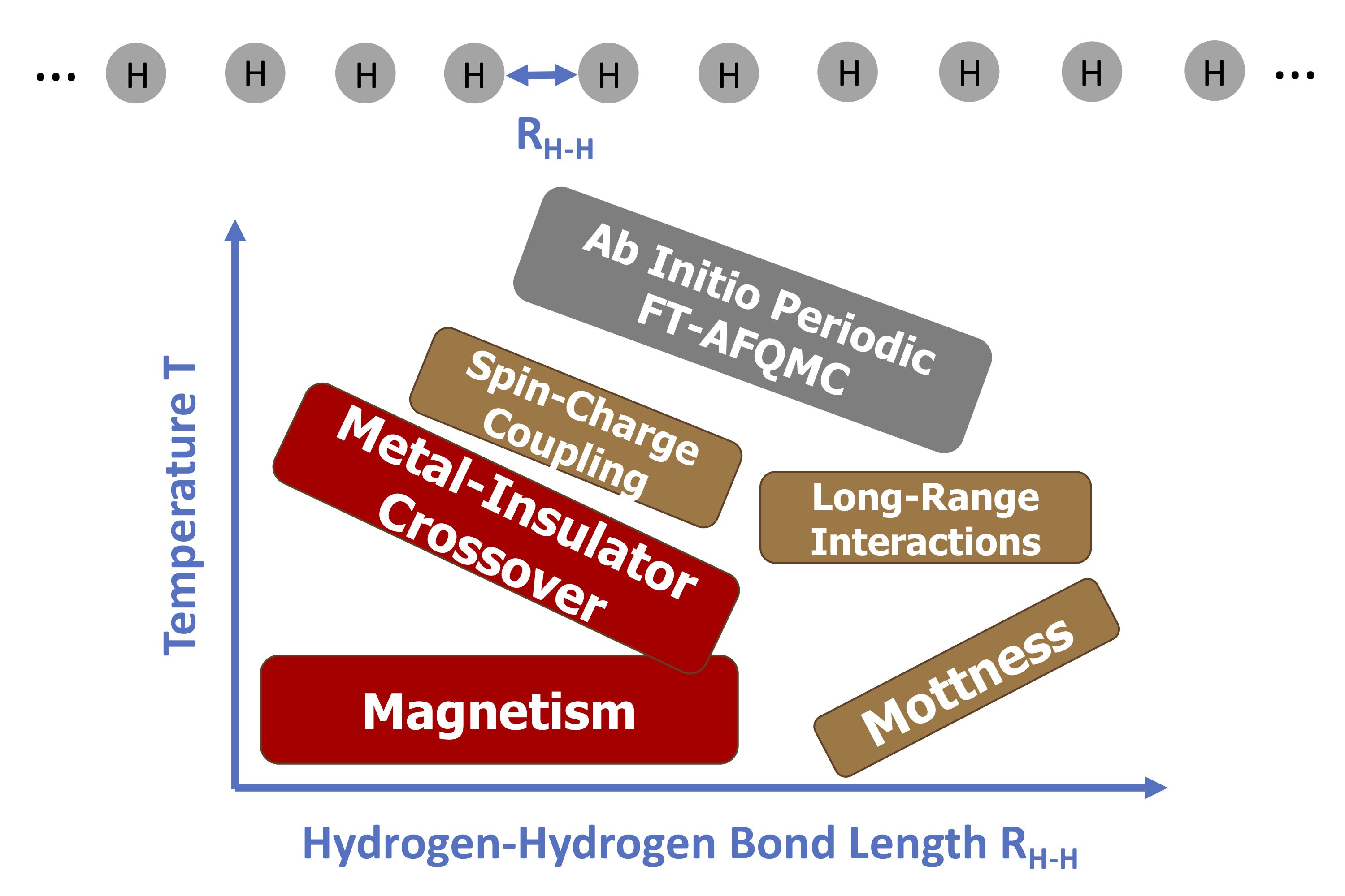
Figure 13: Table of Contents (TOC)

References

- Ramirez and Falicov 1971 Ramirez, R.; Falicov, L. M. Theory of the Phase Transition in Metallic Cerium. Phys. Rev. B 1971, 3, 2425–2430
- Zylbersztejn and Mott 1975 Zylbersztejn, A.; Mott, N. F. Metal-insulator transition in vanadium dioxide. Phys. Rev. B 1975, 11, 4383–4395
- Imada et al. 1998 Imada, M.; Fujimori, A.; Tokura, Y. Metal-insulator transitions. Rev. Mod. Phys. 1998, 70, 1039–1263
- Lichtenstein et al. 2001 Lichtenstein, A. I.; Katsnelson, M. I.; Kotliar, G. Finite-Temperature Magnetism of Transition Metals: An ab initio Dynamical Mean-Field Theory. Phys. Rev. Lett. 2001, 87, 067205
- Orenstein and Millis 2000 Orenstein, J.; Millis, A. J. Advances in the Physics of High-Temperature Superconductivity. Science 2000, 288, 468–474
- Georges et al. 2013 Georges, A.; Medici, L. d.; Mravlje, J. Strong Correlations from Hund‚Äôs Coupling. Annu. Rev. Condens. Matter Phys. 2013, 4, 137–178
- Zhu et al. 2013 Zhu, J.-X.; Albers, R. C.; Haule, K.; Kotliar, G.; Wills, J. M. Site-selective electronic correlation in -plutonium metal. Nat. Commun. 2013, 4, 2644
- Wen and Li 2011 Wen, H.-H.; Li, S. Materials and Novel Superconductivity in Iron Pnictide Superconductors. Annu. Rev. Condens. Matter Phys. 2011, 2, 121–140
- Maeno et al. 1994 Maeno, Y.; Hashimoto, H.; Yoshida, K.; Nishizaki, S.; Fujita, T.; Bednorz, J. G.; Lichtenberg, F. Superconductivity in a layered perovskite without copper. Nature 1994, 372, 532–534
- Drozdov et al. 2015 Drozdov, A. P.; Eremets, M. I.; Troyan, I. A.; Ksenofontov, V.; Shylin, S. I. Conventional superconductivity at 203 kelvin at high pressures in the sulfur hydride system. Nature 2015, 525, 73–76
- Giustino et al. 2007 Giustino, F.; Yates, J. R.; Souza, I.; Cohen, M. L.; Louie, S. G. Electron-Phonon Interaction via Electronic and Lattice Wannier Functions: Superconductivity in Boron-Doped Diamond Reexamined. Phys. Rev. Lett. 2007, 98, 047005
- Kozik et al. 2010 Kozik, E.; Houcke, K. V.; Gull, E.; Pollet, L.; Prokof’ev, N.; Svistunov, B.; Troyer, M. Diagrammatic Monte Carlo for correlated fermions. EPL 2010, 90, 10004
- Zhang 1999 Zhang, S. Finite-temperature monte carlo calculations for systems with fermions. Phys. Rev. Lett. 1999, 83, 2777
- Wang and Xiang 1997 Wang, X.; Xiang, T. Transfer-matrix density-matrix renormalization-group theory for thermodynamics of one-dimensional quantum systems. Phys. Rev. B 1997, 56, 5061–5064
- Georges et al. 1996 Georges, A.; Kotliar, G.; Krauth, W.; Rozenberg, M. J. Dynamical mean-field theory of strongly correlated fermion systems and the limit of infinite dimensions. Rev. Mod. Phys. 1996, 68, 13–125
- Maier et al. 2005 Maier, T.; Jarrell, M.; Pruschke, T.; Hettler, M. H. Quantum cluster theories. Rev. Mod. Phys. 2005, 77, 1027–1080
- Savrasov and Kotliar 2004 Savrasov, S. Y.; Kotliar, G. Spectral density functionals for electronic structure calculations. Phys. Rev. B 2004, 69, 245101
- Kotliar et al. 2006 Kotliar, G.; Savrasov, S. Y.; Haule, K.; Oudovenko, V. S.; Parcollet, O.; Marianetti, C. A. Electronic structure calculations with dynamical mean-field theory. Rev. Mod. Phys. 2006, 78, 865–951
- Sun and Kotliar 2002 Sun, P.; Kotliar, G. Extended dynamical mean-field theory and method. Phys. Rev. B 2002, 66, 085120
- Welden et al. 2016 Welden, A. R.; Rusakov, A. A.; Zgid, D. Exploring connections between statistical mechanics and Green’s functions for realistic systems: Temperature dependent electronic entropy and internal energy from a self-consistent second-order Green’s function. J. Chem. Phys. 2016, 145, 204106
- Kananenka et al. 2016 Kananenka, A. A.; Phillips, J. J.; Zgid, D. Efficient Temperature-Dependent Green’s Functions Methods for Realistic Systems: Compact Grids for Orthogonal Polynomial Transforms. J. Chem. Theory Comput. 2016, 12, 564–571, PMID: 26735685
- Kananenka et al. 2016 Kananenka, A. A.; Welden, A. R.; Lan, T. N.; Gull, E.; Zgid, D. Efficient Temperature-Dependent Green’s Function Methods for Realistic Systems: Using Cubic Spline Interpolation to Approximate Matsubara Green’s Functions. J. Chem. Theory Comput. 2016, 12, 2250–2259, PMID: 27049642
- Sun et al. 2019 Sun, C.; Ray, U.; Cui, Z.-H.; Stoudenmire, M.; Ferrero, M.; Kin-Lic Chan, G. Finite temperature density matrix embedding theory. arXiv e-prints 2019, arXiv:1911.07439
- Marsman et al. 2009 Marsman, M.; Gruneis, A.; Paier, J.; Kresse, G. Second-order Muller‚ Plesset perturbation theory applied to extended systems. I. Within the projector-augmented-wave formalism using a plane wave basis set. J. Chem. Phys. 2009, 130, 184103
- McClain et al. 2017 McClain, J.; Sun, Q.; Chan, G. K.-L.; Berkelbach, T. C. Gaussian-Based Coupled-Cluster Theory for the Ground-State and Band Structure of Solids. J. Chem. Theory Comput. 2017, 13, 1209–1218, PMID: 28218843
- Booth et al. 2013 Booth, G. H.; Grüneis, A.; Kresse, G.; Alavi, A. Towards an exact description of electronic wavefunctions in real solids. Nature 2013, 493, 365–370
- Jha and Hirata 2019 Jha, P. K.; Hirata, S. Finite-Temperature Many-Body Perturbation Theory in the Canonical Ensemble. arXiv e-prints 2019, arXiv:1910.07628
- White and Chan 2018 White, A. F.; Chan, G. K.-L. A Time-Dependent Formulation of Coupled-Cluster Theory for Many-Fermion Systems at Finite Temperature. J. Chem. Theory Comput. 2018, 14, 5690–5700, PMID: 30260642
- Hummel 2018 Hummel, F. Finite temperature coupled cluster theories for extended systems. J. Chem. Theory Comput. 2018, 14, 6505–6514
- Harsha et al. 2019 Harsha, G.; Henderson, T. M.; Scuseria, G. E. Thermofield theory for finite-temperature coupled cluster. J. Chem. Theory Comput. 2019, 15, 6127–6136
- White and Chan 2020 White, A. F.; Chan, G. K. Finite-temperature coupled cluster: Efficient implementation and application to prototypical systems. arXiv preprint arXiv:2004.01729 2020,
- Petras et al. 2020 Petras, H. R.; Ramadugu, S. K.; Malone, F. D.; Shepherd, J. J. Using Density Matrix Quantum Monte Carlo for Calculating Exact-on-Average Energies for ab Initio Hamiltonians in a Finite Basis Set. J. Chem. Theory Comput. 2020, 16, 1029–1038
- Militzer and Driver 2015 Militzer, B.; Driver, K. P. Development of Path Integral Monte Carlo Simulations with Localized Nodal Surfaces for Second-Row Elements. Phys. Rev. Lett. 2015, 115, 176403
- Liu et al. 2018 Liu, Y.; Cho, M.; Rubenstein, B. Ab Initio Finite Temperature Auxiliary Field Quantum Monte Carlo. J. Chem. Theory Comput. 2018, 14, 4722–4732, PMID: 30102856
- Rubenstein et al. 2012 Rubenstein, B. M.; Zhang, S.; Reichman, D. R. Finite-temperature auxiliary-field quantum Monte Carlo technique for Bose-Fermi mixtures. Phys. Rev. A 2012, 86, 053606
- Szabo and Ostlund 1996 Szabo, A.; Ostlund, N. Modern Quantum Chemistry: Introduction to Advanced Electronic Structure Theory; Dover Books on Chemistry; Dover Publications, 1996
- Stella et al. 2011 Stella, L.; Attaccalite, C.; Sorella, S.; Rubio, A. Strong electronic correlation in the hydrogen chain: A variational Monte Carlo study. Phys. Rev. B 2011, 84, 245117
- Hachmann et al. 2006 Hachmann, J.; Cardoen, W.; Chan, G. K.-L. Multireference correlation in long molecules with the quadratic scaling density matrix renormalization group. J. Chem. Phys. 2006, 125, 144101
- Motta et al. 2019 Motta, M.; Genovese, C.; Ma, F.; Cui, Z.-H.; Sawaya, R.; Chan, G. K.; Chepiga, N.; Helms, P.; Jimenez-Hoyos, C.; Millis, A. J., et al. Ground-state properties of the hydrogen chain: insulator-to-metal transition, dimerization, and magnetic phases. arXiv preprint arXiv:1911.01618 2019,
- Motta et al. 2017 Motta, M.; Ceperley, D. M.; Chan, G. K.-L.; Gomez, J. A.; Gull, E.; Guo, S.; Jiménez-Hoyos, C. A.; Lan, T. N.; Li, J.; Ma, F., et al. Towards the solution of the many-electron problem in real materials: equation of state of the hydrogen chain with state-of-the-art many-body methods. Phys. Rev. X 2017, 7, 031059
- Sinitskiy et al. 2010 Sinitskiy, A. V.; Greenman, L.; Mazziotti, D. A. Strong correlation in hydrogen chains and lattices using the variational two-electron reduced density matrix method. J. Chem. Phys. 2010, 133, 014104
- Rusakov and Zgid 2016 Rusakov, A. A.; Zgid, D. Self-consistent second-order Green’s function perturbation theory for periodic systems. J. Chem. Phys. 2016, 144, 054106
- Welden et al. 2016 Welden, A. R.; Rusakov, A. A.; Zgid, D. Exploring connections between statistical mechanics and Green’s functions for realistic systems: Temperature dependent electronic entropy and internal energy from a self-consistent second-order Green’s function. J. Chem. Phys. 2016, 145, 204106
- Lieb and Wu 1994 Lieb, E. H.; Wu, F. Y. Exactly Solvable Models Of Strongly Correlated Electrons; World Scientific, 1994; pp 9–12
- Schulz 1993 Schulz, H. Wigner crystal in one dimension. Phys. Rev. Lett. 1993, 71, 1864
- Gebhard et al. 1994 Gebhard, F.; Girndt, A.; Ruckenstein, A. E. Charge-and spin-gap formation in exactly solvable Hubbard chains with long-range hopping. Phys. Rev. B 1994, 49, 10926
- Hirsch 1984 Hirsch, J. Charge-density-wave to spin-density-wave transition in the extended Hubbard model. Phys. Rev. Lett. 1984, 53, 2327
- Kuroki et al. 1994 Kuroki, K.; Kusakabe, K.; Aoki, H. Phase diagram of the extended attractive Hubbard model in one dimension. Phys. Rev. B 1994, 50, 575
- Glocke et al. 2007 Glocke, S.; Klümper, A.; Sirker, J. Half-filled one-dimensional extended Hubbard model: Phase diagram and thermodynamics. Phys. Rev. B 2007, 76, 155121
- Sun et al. 2017 Sun, Q.; Berkelbach, T. C.; McClain, J. D.; Chan, G. K.-L. Gaussian and plane-wave mixed density fitting for periodic systems. J. Chem. Phys. 2017, 147, 164119
- White et al. 1988 White, S.; Sugar, R.; Scalettar, R. Algorithm for the simulation of many-electron systems at low temperatures. Phys. Rev. B 1988, 38, 11665
- Motta and Zhang 2017 Motta, M.; Zhang, S. Ab Initio Computations of Molecular Systems by the Auxiliary-Field Quantum Monte Carlo Method. arXiv:1711.02242 2017,
- Hirsch 1985 Hirsch, J. E. Two-dimensional Hubbard model: Numerical simulation study. Phys. Rev. B 1985, 31, 4403–4419
- Hirsch 1983 Hirsch, J. E. Discrete Hubbard-Stratonovich transformation for fermion lattice models. Phys. Rev. B 1983, 28, 4059–4061
- Hirsch et al. 1982 Hirsch, J. E.; Sugar, R. L.; Scalapino, D. J.; Blankenbecler, R. Monte Carlo simulations of one-dimensional fermion systems. Phys. Rev. B 1982, 26, 5033
- Zhang and Krakauer 2003 Zhang, S.; Krakauer, H. Quantum Monte Carlo Method using Phase-Free Random Walks with Slater Determinants. Phys. Rev. Lett. 2003, 90, 136401
- McClain et al. 2017 McClain, J.; Sun, Q.; Chan, G. K.-L.; Berkelbach, T. C. Gaussian-based coupled-cluster theory for the ground-state and band structure of solids. J. Chem. Theory Comput. 2017, 13, 1209–1218
- Martin 2004 Martin, R. Electronic Structure: Basic Theory and Practical Methods; Cambridge University Press, 2004
- Sun et al. 2017 Sun, Q.; Berkelbach, T. C.; McClain, J. D.; Chan, G. K.-L. Gaussian and plane-wave mixed density fitting for periodic systems. J. Chem. Phys. 2017, 147, 164119
- Predescu et al. 2003 Predescu, C.; Sabo, D.; Doll, J.; Freeman, D. L. Heat capacity estimators for random series path-integral methods by finite-difference schemes. J. Chem. Phys. 2003, 119, 12119–12128
- Fetter and Walecka 2003 Fetter, A. L.; Walecka, J. D. Quantum theory of many-particle systems; Dover Publications, Inc., 2003
- Callen et al. 1985 Callen, H.; Callen, H.; of Australia. Research Division, N. F. R. C.; Sons, W. . Thermodynamics and an Introduction to Thermostatistics; Wiley, 1985
- Malone et al. 2016 Malone, F. D.; Blunt, N. S.; Brown, E. W.; Lee, D. K. K.; Spencer, J. S.; Foulkes, W. M. C.; Shepherd, J. J. Accurate Exchange-Correlation Energies for the Warm Dense Electron Gas. Phys. Rev. Lett. 2016, 117, 115701
- Toldin and Assaad 2018 Toldin, F. P.; Assaad, F. F. Entanglement Hamiltonian of interacting fermionic models. Phys. Rev. Lett. 2018, 121, 200602
- Blunt et al. 2014 Blunt, N. S.; Rogers, T. W.; Spencer, J. S.; Foulkes, W. M. C. Density-matrix quantum Monte Carlo method. Phys. Rev. B 2014, 89, 245124
- Sun et al. 2018 Sun, Q.; Berkelbach, T. C.; Blunt, N. S.; Booth, G. H.; Guo, S.; Li, Z.; Liu, J.; McClain, J. D.; Sayfutyarova, E. R.; Sharma, S., et al. PySCF: the Python-based simulations of chemistry framework. Wiley Interdiscip. Rev. Comput. Mol. Sci. 2018, 8, e1340
- Liu 2020. https://doi.org/10.26300/hvdk-6836 Liu, Y. Integral Files. Brown University Open Data Collection; Brown Digital Repository. Brown University Library, 2020. https://doi.org/10.26300/hvdk-6836
- Liu 2020. https://doi.org/10.26300/0m74-xp13 Liu, Y. Figures Data. Brown University Open Data Collection; Brown Digital Repository. Brown University Library, 2020. https://doi.org/10.26300/0m74-xp13
- Hubbard 1963 Hubbard, J. Electron correlations in narrow energy bands. Proc. R. Soc. A 1963, 276, 238–257
- Ghosh 1970 Ghosh, D. Electron correlation in an extended Hubbard model. Phys. Lett. A 1970, 32, 429–431
- Rusakov et al. 2018 Rusakov, A. A.; Iskakov, S.; Tran, L. N.; Zgid, D. Self-energy embedding theory (SEET) for periodic systems. J. Chem. Theory Comput. 2018, 15, 229–240
- Shiba 1972 Shiba, H. Thermodynamic Properties of the One-Dimensional Half-Filled-Band Hubbard Model. II: Application of the Grand Canonical Method. Prog. Theor. Phys. 1972, 48, 2171–2186
- Mott 2004 Mott, N. Metal-Insulator Transitions; CRC Press, 2004
- Chitra and Kotliar 2000 Chitra, R.; Kotliar, G. Effect of long range coulomb interactions on the mott transition. Phys. Rev. Lett. 2000, 84, 3678
- Poilblanc et al. 1997 Poilblanc, D.; Yunoki, S.; Maekawa, S.; Dagotto, E. Insulator-metal transition in one dimension induced by long-range electronic interactions. Phys. Rev. B 1997, 56, R1645
- Jördens et al. 2008 Jördens, R.; Strohmaier, N.; Günter, K.; Moritz, H.; Esslinger, T. A Mott insulator of fermionic atoms in an optical lattice. Nature 2008, 455, 204–207
- Scarola et al. 2009 Scarola, V. W.; Pollet, L.; Oitmaa, J.; Troyer, M. Discerning Incompressible and Compressible Phases of Cold Atoms in Optical Lattices. Phys. Rev. Lett. 2009, 102, 135302
- Georges and Krauth 1992 Georges, A.; Krauth, W. Numerical solution of the d= Hubbard model: Evidence for a Mott transition. Phys. Rev. Lett. 1992, 69, 1240
- Georges and Krauth 1993 Georges, A.; Krauth, W. Physical properties of the half-filled Hubbard model in infinite dimensions. Phys. Rev. B 1993, 48, 7167
- Sciolla et al. 2013 Sciolla, B.; Tokuno, A.; Uchino, S.; Barmettler, P.; Giamarchi, T.; Kollath, C. Competition of spin and charge excitations in the one-dimensional Hubbard model. Phys. Rev. A 2013, 88, 063629
- Shen et al. 1991 Shen, Z.-X.; List, R.; Dessau, D.; Wells, B.; Jepsen, O.; Arko, A.; Barttlet, R.; Shih, C.-K.; Parmigiani, F.; Huang, J., et al. Electronic structure of NiO: Correlation and band effects. Phys. Rev. B 1991, 44, 3604
- Kuneš et al. 2007 Kuneš, J.; Anisimov, V.; Skornyakov, S.; Lukoyanov, A.; Vollhardt, D. NiO: correlated band structure of a charge-transfer insulator. Phys. Rev. Lett. 2007, 99, 156404
- Voit 1992 Voit, J. Phase diagram and correlation functions of the half-filled extended Hubbard model in one dimension. Phys. Rev. B 1992, 45, 4027
- Löwdin 1955 Löwdin, P.-O. Quantum theory of many-particle systems. I. Physical interpretations by means of density matrices, natural spin-orbitals, and convergence problems in the method of configurational interaction. Phys. Rev. 1955, 97, 1474
- Mermin and Wagner 1966 Mermin, N. D.; Wagner, H. Absence of ferromagnetism or antiferromagnetism in one-or two-dimensional isotropic Heisenberg models. Phys. Rev. Lett. 1966, 17, 1133
- Ghosh 1971 Ghosh, D. K. Nonexistence of magnetic ordering in the one-and two-dimensional Hubbard model. Phys. Rev. Lett. 1971, 27, 1584
- Malone et al. 2015 Malone, F. D.; Blunt, N. S.; Shepherd, J. J.; Lee, D. K. K.; Spencer, J. S.; Foulkes, W. M. C. Interaction picture density matrix quantum Monte Carlo. J. Chem. Phys. 2015, 143, 044116
- Kwee et al. 2008 Kwee, H.; Zhang, S.; Krakauer, H. Finite-Size Correction in Many-Body Electronic Structure Calculations. Phys. Rev. Lett. 2008, 100, 126404
- Ma et al. 2011 Ma, F.; Zhang, S.; Krakauer, H. Finite-size correction in many-body electronic structure calculations of magnetic systems. Phys. Rev. B 2011, 84, 155130
- Dornheim et al. 2016 Dornheim, T.; Groth, S.; Sjostrom, T.; Malone, F. D.; Foulkes, W.; Bonitz, M. Ab initio Quantum Monte Carlo simulation of the warm dense electron gas in the thermodynamic limit. Phys. Rev. Lett. 2016, 117, 156403
- Brown et al. 2013 Brown, E. W.; Clark, B. K.; DuBois, J. L.; Ceperley, D. M. Path-integral Monte Carlo simulation of the warm dense homogeneous electron gas. Phys. Rev. Lett. 2013, 110, 146405
- He et al. 2019 He, Y.-Y.; Qin, M.; Shi, H.; Lu, Z.-Y.; Zhang, S. Finite-temperature auxiliary-field quantum Monte Carlo: Self-consistent constraint and systematic approach to low temperatures. Phys. Rev. B 2019, 99, 045108