Grammar-Compressed Indexes
with Logarithmic Search Time

Abstract

Let a text $T[1..n]$ be the only string generated by a context-free grammar with $g$ (terminal and nonterminal) symbols, and of size $G$ (measured as the sum of the lengths of the right-hand sides of the rules). Such a grammar, called a grammar-compressed representation of $T$, can be encoded using essentially $G\lg g$ bits. We introduce the first grammar-compressed index that uses $O(G\lg n)$ bits and can find the $occ$ occurrences of patterns $P[1..m]$ in time $O((m^{2}+occ)\lg G)$. We implement the index and demonstrate its practicality in comparison with the state of the art, on highly repetitive text collections.

1 Introduction and Related Work

Grammar-based compression is an active area of research since at least the seventies [CRA76, Sto77, ZL78, SS82]. A given sequence $T[1..n]$ over alphabet $[1..\sigma]$ is replaced by a hopefully small (context-free) grammar $\mathcal{G}$ that generates just the string $T$. Let $g$ be the number of grammar symbols, counting terminals and nonterminals. Let $G=|\mathcal{G}|$ be the size of the grammar, measured as the sum of the lengths of the right-hand sides of the rules. Then a basic grammar-compressed representation of $T$ requires essentially $G\lg g$ bits, instead of the $n\lg\sigma$ bits required by a plain representation. It always holds $G\geq\lg n$, and indeed $G$ can be as small as $O(\lg n)$ in extreme cases; consider $T=a^{n}$.

Grammar-based methods can achieve universal compression [KY00]. Unlike statistical methods, which exploit frequencies to achieve compression, grammar-based methods exploit repetitions in the text, and thus they are especially suitable for compressing highly repetitive sequence collections. These collections, containing long identical substrings that are possibly far away from each other, arise when managing software repositories, versioned documents, transaction logs, periodic publications, and computational biology sequence databases, among others. Statistical compression is helpless to exploit this sort of long-range repetitiveness [KN13, Nav12].

Finding the smallest grammar $\mathcal{G}^{*}$ that represents a given text $T$ is NP-complete [Sto77, SS82, Ryt03, CLL⁺05]. Moreover, the size $G^{*}$ of the smallest grammar is never smaller than the number $z$ of phrases in a Lempel-Ziv parse [LZ76] of $T$. A simple method to achieve an $O(\lg n)$-approximation to the smallest grammar size is to parse $T$ using Lempel-Ziv and then convert it into a grammar [Ryt03]. More sophisticated approximations [Ryt03, CLL⁺05, Jez15, Jez16] achieve ratio $O(\lg(n/G^{*}))$ (indeed, they obtain size $G=O(z\lg(n/z))$). Recently, it has been shown that this is not far from the lower bound, as there are sequence families where $G^{*}=\Omega(z\lg n/\lg\lg n)$ [HLR16].

The known approximation ratios of popular grammar compressors such as LZ78 [ZL78], Re-Pair [LM00] and Sequitur [NMWM94], instead, are much larger than the optimal [CLL⁺05, HLR16]. Still, some of those methods (in particular Re-Pair) perform very well in practice, both in classical and repetitive settings.

On the other hand, unlike Lempel-Ziv, grammar compression allows one to decompress arbitrary substrings of $T$ in logarithmic time [GKPS05, BLR⁺15, BPT15]. The most recent results extract any $T[p..p+\ell-1]$ in time $O(\ell+\lg n)$ [BLR⁺15] and even $O(\ell/\lg_{\sigma}n+\lg n)$ [BPT15], which is close to optimal [VY13]. Unfortunately, those representations require $O(G\lg n)$ bits, possibly proportional but in practice many times the size of the output of a grammar compressor.

More ambitious than just extracting substrings from $T$ is to ask for indexed searches, that is, finding the $occ$ occurrences in $T$ of a given pattern $P[1..m]$. Self-indexes are compressed text representations that support both operations, extract $T[p..p+\ell-1]$ and locate the occurrences of a pattern $P[1..m]$, in time sublinear (and usually polylogarithmic) in $n$. They have appeared in the last decade [NM07], and have focused mostly on statistical compression. As a result, they work well on classical texts, but not on repetitive collections [MNSV10]. Some of those self-indexes have been adapted to such repetitive collections [MNSV10, NPL⁺13, NPC⁺13, DJSS14, BGG⁺14, BCG⁺15, GNP18], but they do not reach the compression ratio of the best grammar-based methods.

Searching for patterns on grammar-compressed text has been faced mostly in sequential form [AB92], that is, scanning the whole grammar. The best result [KMS⁺03] achieves time $O(G+m^{2}+occ)$. This may be $o(n)$, but is still linear in the size of the compressed text. There exist a few self-indexes based on LZ78-like compression [FM05, RO08, ANS12], but LZ78 is among the weakest grammar-based compressors. In particular, LZ78 has been shown not to be competitive on highly repetitive collections [MNSV10].

The only self-index supporting general grammar compressors [CN10] operates on “straight-line programs” (SLPs), where the right hands of the rules are of length 1 or 2. Given such a grammar they achieve, among other tradeoffs, $3g\lg g+g\lg n$ bits of space and $O(m(m+h)\lg^{2}g)$ search time, where $h\leq g$ is the height of the parse tree of the grammar. A general grammar of $g$ symbols and size $G$ can be converted into an SLP by adding at most $G-2g$ symbols and/or rules.

More recently, a self-index based on Lempel-Ziv compression was developed [KN13]. It uses $z\lg z+2z\lg n+O(z\lg\sigma)$ bits of space and searches in time $O(m^{2}\bar{h}+(m+occ)\lg z)$, where $\bar{h}\leq z$ is the nesting of the parsing. Extraction requires $O(\ell\,\bar{h})$ time. Experiments on repetitive collections [CFMPN10, CFMPN16] showed that the grammar-based compressor [CN10] can outperform the (by then) best classical self-index adapted to repetitive collections [MNSV10] but, at least that particular implementation, was not competitive with the Lempel-Ziv-based self-index [KN13].

The search times in both self-indexes depend on $h$ or $\bar{h}$. This is undesirable as both are only bounded by $g$ or $z$, respectively. As mentioned, this kind of dependence has been removed for extracting text substrings [BLR⁺15], at the cost of using $O(G\lg n)$ further bits.

There have also been combinations of grammar-based and Lempel-Ziv-based methods [GGK⁺12, GGK⁺14, BEGV18, CE18], yet (1) none of those is implemented, (2) the constant factors multiplying their space complexities are usually large, (3) they cannot be built on a given arbitrary grammar. They use at least $O(z\log(n/z)\log n)$ bits (which is an upper bound to our space complexity) and can search as fast as in $O(m+\log^{\epsilon}z+occ(\log^{\epsilon}z+\log\log n))$ time for any constant $\epsilon>0$ [CE18], decreasing to $O(m+occ\log\log n)$ time with $O(z\log(g/z)\log\log z\log n)$ bits of space [BEGV18]. Gagie et al. [GGK⁺12] can depart from any given grammar, but add some extra space so that, within $O(G\log n+z\log\log z\log n)$ bits, they can search in time $O(m^{2}+(m+occ)\log\log n)$.

Recently, Navarro and Prezza [NP19] introduced a self-index of $O(\gamma\lg(n/\gamma)\lg n)$ bits, where $\gamma\leq z\leq G$ is the size of any attractor of $T$ (which lower-bounds many other repetitiveness measures). They can search in time $O(m\log n+occ\log^{\epsilon}n)$. This result is theoretically appealing, but again suffers from the drawbacks (1)–(3) above, and still its size dominates only an upper bound on $G$.

In this article we introduce the first (as of the time of conference publication [CN12], and still the only) grammar-based self-index that can be built from any given grammar of size $G$, which uses $O(G\lg n)$ bits and whose search time depends only logarithmically on $n$, independently of the grammar height. In addition, we give a practical implementation of the index and compare it with different state-of-the-art indexes on repetitive collections, showing that our index is also practical. In fact, the ability of our index to build on any grammar has an important practical value, because it can be built on top of compressors like RePair, which perform extremely well in practice.

The following theorem summarizes its properties; we note that the search time can be simplified to $O((m^{2}+occ)\lg G)$ because $\lg\lg n\leq\lg G$.

Theorem 1.1

Let a sequence $T[1..n]$ be represented by a context-free grammar with $g$ symbols, size $G$ and height $h$. Then, for any $0<\epsilon\leq 1$, there exists a data structure using at most $G\lg n+2G\lg g+\epsilon\,g\lg g+o(G\lg g)+O(G)$ bits that finds the $occ$ occurrences of any pattern $P[1..m]$ in $T$ in time $O((m^{2}/\epsilon)\lg\lg n+(m+occ)(1/\epsilon+\lg g/\lg\lg g))$. It can extract any substring of length $\ell$ from $T$ in time $O(\ell+h\lg(G/h))$. The structure can be built in $O(n+G\lg G)$ time and $O(n\lg n)$ bits of working space.

Note that the extraction time still depends on the grammar height. To improve it, we can include the structure of Belazzougui et al. [BPT15], which adds $O(G\lg n)$ bits. Within that space we derive a coarser version of our result.

Corollary 1

Let a sequence $T[1..n]$ over alphabet $[1..\sigma]$ be represented by a context-free grammar with $g$ symbols and of size $G$. Then there exists an index requiring $O(G\lg n)$ bits that finds the $occ$ occurrences of any pattern $P[1..m]$ in $T$ in time $O(m^{2}+(m+occ)\lg^{\epsilon}g)$, for any constant $\epsilon>0$, and extracts any substring of length $\ell$ from $T$ in time $O(\ell/\lg_{\sigma}n+\lg n)$.

In the rest of the article we describe our structure. First, we preprocess the grammar to enforce several invariants useful to ensure our time complexities. Then we use a data structure for binary relations [BCN13] to find the “primary” occurrences of $P$, that is, those formed when concatenating symbols in the right hand side of a rule. To get rid of the factor $h$ in this part of the search, we extend a technique [GKPS05] to extract the first $m$ symbols of the expansion of any nonterminal in time $O(m)$. To find the “secondary” occurrences (i.e., those that are found as the result of the nonterminal containing primary occurrences being mentioned elsewhere), we use a pruned representation of the parse tree of $T$. This tree is traversed upwards for each secondary occurrence to report. The grammar invariants introduced ensure that those traversals amortize to a constant number of steps per occurrence reported. In this way we get rid of the factor $h$ on the secondary occurrences too.

We also show that our structure is practical. In Section 8 we implement the index of Theorem 1.1 and show that it outperforms the preceding grammar-based index [CN10], even in its optimized form [CFMPN16], and it becomes a valid space/time tradeoff to the Lempel-Ziv based self-index [KN13] (also in optimized form [CFMPN16]). Our expermental results show that, while the technique to speed up the extraction [GKPS05] does not have an impact in practice, the idea to amortize the cost of finding the secondary occurrences does speed up the index significantly in practice.

The main differences with our conference version [CN12] are improved theoretical complexities, the whole implementation and experimental results, and an expanded and improved writing.

2 Basic Concepts

2.1 Sequence Representations

Our data structures use succinct representations of sequences. Given a sequence $S[1..N]$, over the alphabet $\Sigma$, we need to support the following operations:

• $\mathit{access}(S,i)$ retrieves the symbol $S[i]$;

• $\mathit{rank}_{a}(S,i)$ counts the number of occurrences of $a$ in $S[1..i]$;

• $\mathit{select}_{a}(S,j)$ computes the position where the $j$th $a$ appears in $S$.

For the case $|\Sigma|=2$ (i.e., bitmaps), all the operations can be supported in $N+o(N)$ bits and constant time [Cla96]. Raman et al. [RRR07] proposed two compressed representations that are useful when the number $N_{1}$ of $1$s in $S$ is small. One is the “fully indexable dictionary” (FID). It takes $N_{1}\lg\frac{N}{N_{1}}+O(N_{1})+o(N)$ bits of space and supports all the operations in constant time. A weaker one is the “indexable dictionary” (ID), which takes $N_{1}\lg\frac{N}{N_{1}}+O(N_{1}+\lg\lg N)$ bits of space and supports in constant time queries $\mathit{access}(S,i)$, $\mathit{rank}(S,i)$ if $S[i]=1$, and $\mathit{select}_{1}(S,j)$.

For general sequences, we will use a representation [BN15] that requires $N\lg|\Sigma|+o(N\lg|\Sigma|)$ bits and solves $\mathit{access}(S,i)$ in $O(1)$ time and $\mathit{select}(S,j)$ in any time in $\omega(1)$ (as a function of $|\Sigma|$), or vice versa; $\mathit{rank}(S,i)$ takes time $O(\lg\lg_{w}|\Sigma|)$, on a RAM machine of $w$ bits.

2.2 Labeled Binary Relations

A labeled binary relation is a binary relation $\mathcal{R}\subseteq A\times B$, where $A=[1..n_{1}]$ and $B=[1..n_{2}]$, augmented with a function $\mathcal{L}:A\times B\rightarrow L\cup\{\perp\}$, $L=[1..\ell]$, that defines labels for each pair in $\mathcal{R}$, and $\perp$ for pairs that are not in $\mathcal{R}$. Let us identify $A$ with the columns and $B$ with the rows in a table. In our case, each element of $A$ will be associated with exactly one element of $B$, so $|\mathcal{R}|=n_{1}$. We augment a representation of unlabeled binary relations [BCN13] with a plain string $S_{\mathcal{L}}[1..n_{1}]$ on alphabet $[1..\ell]$, where $S_{\mathcal{L}}[i]$ is the label of the pair of column $i$. The total space of this structure is $n_{1}(\lg n_{2}+\lg\ell)+o(n_{1}\lg n_{2})$ bits. With this representation we can answer, among others, the following queries of interest in this article:

1. Find the label of the element $b$ associated with a given $a$, $S_{\mathcal{L}}[a]$, in $O(1)$ time.

2. Given $a_{1},a_{2},b_{1}$, and $b_{2}$, enumerate the $k$ pairs $(a,b)\in\mathcal{R}$ such that $a_{1}\leq a\leq a_{2}$ and $b_{1}\leq b\leq b_{2}$, in time $O((k+1)(1+\lg n_{2}/\lg\lg(n_{1}+n_{2})))$.

2.3 Succinct Tree Representations

There are many representations for trees $\mathcal{T}$ with $N$ nodes that take $2N+o(N)$ bits of space. In this paper we use one called Fully-Functional (FF) [NS14], which in particular answers in constant time the following operations (node identifiers $v$ are associated with a position in $[1..2N]$):

• $\mathit{node}_{\mathcal{T}}(p)$ is the node with preorder number $p$;

• $\mathit{preorder}_{\mathcal{T}}(v)$ is the preorder number of node $v$;

• $\mathit{leafrank}_{\mathcal{T}}(v)$ is the number of leaves to the left of $v$;

• $\mathit{leafselect}_{\mathcal{T}}(j)$ is the $j$th leaf;

• $\mathit{intrank}_{\mathcal{T}}(v)$ is the number of internal nodes before $v$, in preorder;

• $\mathit{intselect}_{\mathcal{T}}(j)$ is the $j$th internal node, in preorder;

• $\mathit{numleaves}_{\mathcal{T}}(v)$ is the number of leaves below $v$;

• $\mathit{parent}_{\mathcal{T}}(v)$ is the parent of $v$;

• $\mathit{child}_{\mathcal{T}}(v,k)$ is the $k$th child of $v$;

• $\mathit{nextsibling}_{\mathcal{T}}(v)$ is the next sibling of $v$;

• $\mathit{degree}_{\mathcal{T}}(v)$ is the number of children of $v$;

• $0pt_{\mathcal{T}}(v)$ is the depth of $v$; and

• ${\mathit{level}\textrm{-}\mathit{ancestor}}_{\mathcal{T}}(v,k)$ is the $k$th ancestor of $v$.

The FF representation is obtained by traversing the tree in DFS order and appending to a bitmap a $1$ when we arrive at a node, and a $0$ when we leave it. The operations $\mathit{leafrank}$, $\mathit{leafselect}$, $\mathit{intrank}$, and $\mathit{intselect}$ are not discussed so widely in the literature. In the FF sequence $F[1..2N]$, each internal node starts with a bit $1$ followed by another $1$, and each leaf is represented by a $1$ followed by a $0$. The same mechanisms described in Section 2.1 to support $\mathit{rank}$ and $\mathit{select}$ for $0$s and $1$s on bitmaps are easily extended to support two-bit operations, within $o(N)$ extra bits. Therefore, we implement $\mathit{leafrank}(i)=\mathit{rank}_{10}(F,i-1)$, $\mathit{leafselect}(j)=\mathit{select}_{10}(F,j)$, $\mathit{intrank}(i)=\mathit{rank}_{11}(F,i-1)$, and $\mathit{intselect}(j)=\mathit{select}_{11}(F,j)$, all in constant time.

3 Preprocessing the Grammar

We will work on a given context-free grammar $\mathcal{G}$ that generates a single string $T[1..n]$ over alphabet $\Sigma=[1..\sigma]$, formed by $g$ (terminal and nonterminal) symbols. The $\sigma\leq g$ terminal symbols come from an alphabet $\Sigma=[1..\sigma]$, and then $\mathcal{G}$ contains $g-\sigma$ rules of the form $X_{i}\rightarrow\alpha_{i}$, exactly one per nonterminal. The sequence $\alpha_{i}$, called the right-hand side of the rule, is the sequence of terminal and non-terminal symbols generated by $X_{i}$ (without recursively unrolling rules). We call $G=\sum|\alpha_{i}|$ the size of $\mathcal{G}$. Note it holds $\sigma\leq G$, since the terminals must appear in the right-hand sides. We assume all the nonterminals are used to generate the string; otherwise unused rules can be found and dropped in $O(G)$ time. The grammar cannot have loops since it generates a finite string $T$.

Let $X_{s}$ be always the start symbol (despite of successive symbol renamings). We call $\mathcal{F}(X_{i})$ the single string generated by $X_{i}$, that is $\mathcal{F}(a)=a$ for terminals $a$ and $\mathcal{F}(X_{i})=\mathcal{F}(X_{i_{1}})\cdots\mathcal{F}(X_{i_{k}})$ for nonterminals $X_{i}\rightarrow X_{i_{1}}\ldots X_{i_{k}}$. The grammar $\mathcal{G}$ generates the text $T=\mathcal{L}(\mathcal{G})=\mathcal{F}(X_{s})$.

For the purpose of building our index, we preprocess $\mathcal{G}$ as follows.

• First, for each terminal symbol $a\in\Sigma$ present in $\mathcal{G}$ we create a rule $X_{a}\rightarrow a$, and replace all other occurrences of $a$ in the grammar by $X_{a}$. As a result, the grammar contains exactly $g$ nonterminal symbols $\mathcal{X}=\{X_{1},\ldots,X_{g}\}$, each associated with a rule $X_{i}\rightarrow\alpha_{i}$, where $\alpha_{i}\in\Sigma$ or $\alpha_{i}$ is a sequence of elements in $\mathcal{X}$.

• Any rule that generates just one single nonterminal $X_{i}\rightarrow X_{j}$, or the empty string, $X_{i}\rightarrow\varepsilon$, is removed by replacing $X_{i}$ by $X_{j}$ or by $\varepsilon$ everywhere. This decreases $g$ without increasing $G$.

• We further preprocess $\mathcal{G}$ to enforce the property that any nonterminal $X_{i}$, except $X_{s}$ and those $X_{a}\rightarrow a\in\Sigma$, must be mentioned in at least two right-hand sides. We traverse the rules of the grammar, count the occurrences of each symbol, and then rewrite the rules, so that only the rules of those $X_{i}$ appearing more than once (or the excepted symbols) are preserved, and as we rewrite their right-hand sides, we replace any (non-excepted) $X_{i}$ that appears once by its right-hand side $\alpha_{i}$. This transformation takes $O(G)$ time and can only reduce $G$ and $g$.

• Our last preprocessing step, and the most expensive one, is to renumber the nonterminals so that $i<j\Leftrightarrow\mathcal{F}(X_{i})^{rev}<\mathcal{F}(X_{j})^{rev}$, where $S^{rev}$ is string $S$ read backwards (the purpose of this renumbering will be apparent later). The sorting can be done in time $O(n+g\lg g)$ and $O(n\lg n)$ bits of space, following the same approach as in previous work [CN10]. This process dominates the construction time.

From now on, $g$ will refer to the number of rules in the transformed grammar $\mathcal{G}$ (i.e., the number of terminal and nonterminal symbols in the original grammar, minus possible reductions). Instead, $G$ will still be the size of the original grammar (the transformed one has size at most $G+\sigma$).

4 Main Index Structure

We define a structure that will be key in our index.

Definition 1

The grammar tree of $\mathcal{G}$ is a general tree $\mathcal{T}_{\mathcal{G}}$ with nodes labeled in $\mathcal{X}$. Its root is labeled $X_{s}$ and its topology is obtained by pruning the parse tree of $T$ with two rules: (1) in a left-to-right DFS traversal, in each noded except the first time a nonterminal $X_{i}$ is found, its subtree is pruned and the node becomes a leaf; (2) whenever $X_{a}\rightarrow a$ is found, it is pruned too, leaving $X_{a}$ as a leaf. We say that each $X_{i}$ is defined in the only internal node of $\mathcal{T}_{\mathcal{G}}$ labeled $X_{i}$.

Since each right-hand side $\alpha_{i}\not\in\Sigma$ is written once in the tree as the children of $X_{i}$, and the root $X_{s}$ is written once, the total number of nodes in $\mathcal{T}_{\mathcal{G}}$ is $G+1$. The number of internal nodes is $g-\sigma$, and the number of leaves is $G+1-g+\sigma$. Figure 1 shows the reordering and grammar tree for a grammar generating the string "alabaralalabarda".

The grammar tree partitions $T$ in a way that is useful for finding occurrences, using a concept that dates back to Kärkkäinen [Kär99].

Definition 2

Let $X_{l_{1}},X_{l_{2}},\ldots$ be the nonterminals labeling the consecutive leaves of $\mathcal{T}_{\mathcal{G}}$. Let $T_{i}=\mathcal{F}(X_{l_{i}})$, then $T=T_{1}T_{2}\ldots$ is a partition of $T$ according to the leaves of $\mathcal{T}_{\mathcal{G}}$. We say that an occurrence of a pattern $P$ is primary relatively to the given partition if it spans more than one $T_{i}$. The other occurrences are called secondary.

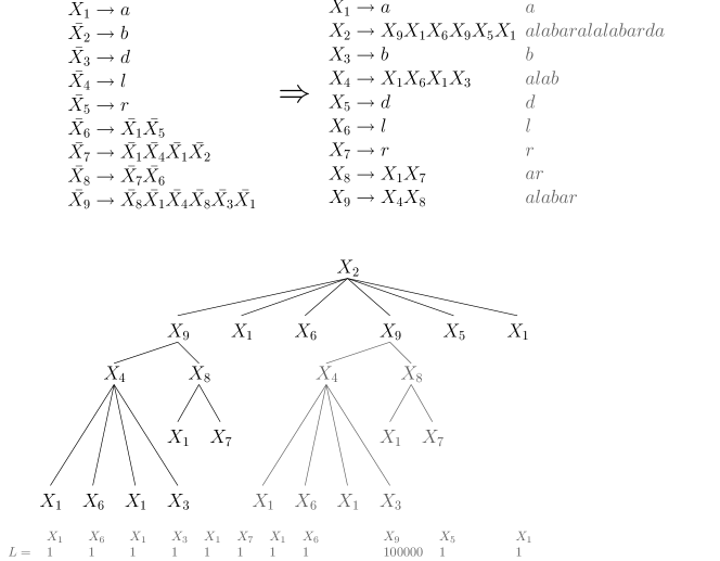
Figure 1: At the top left, a grammar $\mathcal{G}$ generating string "alabaralalabarda". At the top right, our reordering of the grammar and strings $\mathcal{F}(X_{i})$. On the bottom, the grammar tree $\mathcal{T}_{\mathcal{G}}$ in black; the whole parse tree includes also the grayed part. Below the tree we show our bitmap $L$ (Section 5.2).

Our self-index will represent $\mathcal{G}$ using two main components. One represents the grammar tree $\mathcal{T}_{\mathcal{G}}$ using an FF representation (Section 2.3) and a sequence of labels (Section 2.1). This will be used to extract the text and decompress rules. When augmented with a secondary trie $\mathcal{T}_{S}$ storing leftmost/rightmost paths in $\mathcal{T}_{\mathcal{G}}$, the representation will expand any prefix/suffix of a rule in optimal time [GKPS05].

The second component in our self-index corresponds to a labeled binary relation (Section 2.2), where $B=\mathcal{X}$ and $A$ is the set of proper suffixes starting at positions $j+1$ of rules $\alpha_{i}$: $(\alpha_{i}[j],\alpha_{i}[j+1..])$ will be related for all $X_{i}\rightarrow\alpha_{i}$ and $1\leq j<|\alpha_{i}|$. The labels are numbers in the range $[1..G+1]$; we specify their meaning later. This binary relation will be used to find the primary occurrences of the search pattern. Secondary occurrences will be tracked in the grammar tree.

5 Extracting Text

We first describe a simple structure that extracts the prefix of length $\ell$ of any rule in $O(\ell+h)$ time. We then augment this structure to support extracting any substring of length $\ell$ in time $O(\ell+h\lg(G/h))$, and finally augment it further to retrieve the prefix or suffix of length $\ell$ of any rule in optimal $O(\ell)$ time. This last result is fundamental for supporting searches, and is obtained by extending the structure proposed by Gasieniec et al. [GKPS05] for SLPs to general context-free grammars. The improvement does not work for extracting arbitrary substrings, as in that case one has to find first the nonterminals that must be expanded. This subproblem is not easy to solve, especially within little space [BLR⁺15].

As said, we represent the topology of the grammar tree $\mathcal{T}_{\mathcal{G}}$ using FF (Section 2.3), using $O(G)$ bits. The sequence of labels associated with the tree nodes is stored in preorder in a sequence $X[1..G+1]$ using $G\log g+o(G\log g)$ bits with the representation described in Section 2.1, where we choose constant time for $\mathit{access}(X,i)=X[i]$ and $O(\lg\lg_{w}G)$ time for $\mathit{select}_{a}(X,j)$.

We also store a bitmap $Y[1..g]$ that marks the rules of the form $X_{i}\rightarrow a\in\Sigma$ with $1$s. Since the rules have been renumbered in (reverse) lexicographic order, every time we find a rule $X_{i}$ such that $Y[i]=1$, we can determine the terminal symbol it represents as $a=\mathit{rank}_{1}(Y,i)$ in constant time. In our example of Figure 1 this bitmap is $Y=101011100$.

5.1 Expanding Prefixes of Rules

Expanding a rule $X_{i}$ that does not correspond to a terminal is done as follows. By the definition of $\mathcal{T}_{\mathcal{G}}$, the first left-to-right occurrence of $X_{i}$ in sequence $X$ corresponds to the definition of $X_{i}$; all the others are leaves in $\mathcal{T}_{\mathcal{G}}$. Therefore, $v=\mathit{node}_{\mathcal{T}_{\mathcal{G}}}(\mathit{select}_{X_{i}}(X,1))$ is the node in $\mathcal{T}_{\mathcal{G}}$ where $X_{i}$ is defined. We then traverse the subtree rooted at $v$ in DFS order. Every time we reach a leaf $u$, we compute its label $X_{j}=X[\mathit{preorder}_{\mathcal{T}_{\mathcal{G}}}(u)]$, and either output a terminal if $Y[j]=1$ or recursively expand $X_{j}$. This is in fact a traversal of the parse tree starting at node $v$, using the grammar tree instead. The traversal to extract the first $\ell$ terminals takes $O(\ell+h_{v})$ steps, where $h_{v}\leq h$ is the height of the parsing subtree rooted at $v$. In particular, if we extract the whole sequence $\mathcal{F}(X_{i})$, we perform $O(\ell)=O(\mathcal{F}(X_{i}))$ steps, since we have removed unary paths in the preprocessing of $\mathcal{G}$ and thus $v$ has $\mathcal{F}(X_{i})>h_{v}$ leaves in the parse tree. The only obstacle to having constant-time steps are the queries $\mathit{select}_{X_{i}}(X,1)$. As these are only for the position 1, they correspond to finding the internal node of $\mathcal{T}_{\mathcal{G}}$ that defines $X_{i}$. We then store a permutation $\pi[1..g-\sigma]$ so that $X_{i}$ is defined at the node $\mathit{intselect}_{\mathcal{T}_{\mathcal{G}}}(\pi[\mathit{rank}_{0}(Y,i)])$, which is computed in constant time using $g\lg g$ bits for $\pi$.

The total space required for $\mathcal{T}_{\mathcal{G}}$, considering the FF representation, sequence $X$, bitmap $Y$, and permutation $\pi$, is $G\lg g+g\lg g+o(G\lg g)+O(G)$ bits. We reduce the space to $G\lg g+\epsilon\,g\lg g+o(G\lg g)+O(G)$, for any $0<\epsilon\leq 1$, by removing some redundancy: We form a reduced sequence $X^{\prime}[1..G-g+\sigma+1]$ where the labels of the internal nodes are removed. We can still access any $X[i]=X^{\prime}[\mathit{leafrank}_{\mathcal{T}_{\mathcal{G}}}(v)+1]$, with $v=\mathit{node}_{\mathcal{T}_{\mathcal{G}}}(i)$, if $v$ is a leaf. If $v$ is an internal node, we have $X[i]=\mathit{select}_{0}(Y,\pi^{-1}[\mathit{intrank}_{\mathcal{T}_{\mathcal{G}}}(v)+1])$. We can also support general $\mathit{select}$ on $X$: $\mathit{select}_{X_{i}}(X,j)=\mathit{preorder}_{\mathcal{T}_{\mathcal{G}}}(\mathit{leafselect}_{\mathcal{T}_{\mathcal{G}}}(\mathit{select}_{X_{i}}(X^{\prime},j-1)))$ for $j>1$.

Thus, we can use $X^{\prime}$ instead of $X$, at the cost of having to compute $\pi^{-1}$. To do this, we use the representation of Munro et al. [MRRR12] that takes $(1+\epsilon)g\lg g$ bits and computes any $\pi[i]$ in constant time and any $\pi^{-1}[j]$ in time $O(1/\epsilon)$. This yields the promised space. The time to access $X[i]$ is now $O(1/\epsilon)$. Although this will have an impact later, we note that for extraction we only access $X$ at leaf nodes, where it takes constant time.

5.2 Extracting Arbitrary Substrings

In order to extract any given substring of $T$, we add a bitmap $L[1..n]$ that marks with a $1$ the first position of each $T_{i}$ in $T$ (see Figure 1). We can then compute the starting position of any node $v\in\mathcal{T}_{\mathcal{G}}$ as $p(v)=\mathit{select}_{1}(L,\mathit{leafrank}_{\mathcal{T}_{\mathcal{G}}}(v)+1)$.

To extract $T[p..p+\ell-1]$, we binary search the children of the root of $\mathcal{T}_{\mathcal{G}}$, to find the child $u$ covering position $p$. If $u$ is a leaf representing a nonterminal, we go to its definition $v\in\mathcal{T}_{\mathcal{G}}$, translate position $p$ to the area below the new node $v$ (i.e., $p$ becomes $p-p(u)+p(v)$), and continue recursively from $v$. At some point we reach the terminal node $X_{i}\rightarrow a$ covering position $p$, and from there on we extract the symbols rightwards. Just as before, the total number of steps is $O(\ell+h)$. Yet, the $h$ steps require binary searches. As there are at most $h$ binary searches among the children of different tree nodes, and there are $G+1$ nodes, at worst the binary searches cost $O(h\lg(G/h))$. The total cost is $O(\ell+h\lg(G/h))$.

The number of $1$s in $L$ is at most $G$. Since we only need $\mathit{select}_{1}$ on $L$, we can use an ID representation (Section 2.1), requiring $G\lg(n/G)+O(G+\lg\lg n)=G\lg(n/G)+O(G)$ bits (since $G\geq\lg n$ in any grammar). The total space then becomes $G\lg g+G\lg(n/G)+\epsilon\,g\lg g+o(G\lg g)+O(G)$ bits.

Instead, if we implement $L$ with an Elias-Fano structure [Eli74, Fan71], and augment each sub-universe of size $n/G$ with a sampled predecessor data structure, we use $G\lg(n/G)+o(G\lg n)$ bits for $L$ and can solve $rank_{1}$ queries on $L$ in time $O(\lg\lg(n/G))$ (cf. [BN15, Sec. 4.2]). Thus, instead of doing successive binary searches in the path towards the leaf covering $p$, we compute the area of that leaf directly with $1+rank_{1}(L,p)$. Therefore the total time becomes $O(h\lg\lg(n/G))$, because there can still be $h$ jumps to other parts of the tree. We omit this results for simplicity.

5.3 Optimal Expansion of Rule Prefixes and Suffixes

Our improved version builds on the proposal by Gasieniec et al. [GKPS05]. We extend their representation to handle general grammars instead of only SLPs. Using their notation, call $S(X_{i})$ the string of labels of the nodes in the path from any node labeled $X_{i}$ to its leftmost leaf in the parse tree (we take as leaves the nonterminals $X_{a}\in\mathcal{X}$ with $X_{a}\rightarrow a$, not the terminals $a\in\Sigma$). We insert all the strings $S(X_{i})^{rev}$ into a trie $\mathcal{T}_{S}$. Note that each symbol $X_{i}$ appears only once in $\mathcal{T}_{S}$ [GKPS05], thus $\mathcal{T}_{S}$ has $g$ nodes. Again, we represent the topology of $\mathcal{T}_{S}$ using FF. Its sequence of labels $X_{S}[1..g]$ turns out to be a permutation of $[1..g]$. We represent it once again with the structure [MRRR12] that takes $(1+\epsilon)g\lg g$ bits and computes any $X_{S}[i]$ in constant time and any $X_{S}^{-1}[j]$ in time $O(1/\epsilon)$.

We can determine the first terminal in the expansion of $X_{i}$, which labels node $v\in\mathcal{T}_{S}$, as follows. Since the last symbol in $S(X_{i})$ is a nonterminal $X_{a}$ with $X_{a}\rightarrow a$ for some $a\in\Sigma$, it follows that $X_{i}$ descends in $\mathcal{T}_{S}$ from $X_{a}$, which is a child of the root. This node is $v_{a}={\mathit{level}\textrm{-}\mathit{ancestor}}_{\mathcal{T}_{S}}(v,0pt_{\mathcal{T}_{S}}(v)-1)$. Then $a=\mathit{rank}_{1}(Y,X_{S}[\mathit{preorder}_{\mathcal{T}_{S}}(v_{a})])$.

Figure 2 shows an example of this query in the trie for the grammar presented in Figure 1.

Figure 2: Example of the trie of leftmost paths for the grammar of Figure 1. The arrow pointing from $X_{2}$ to $X_{1}$ illustrates the procedure to determine the first terminal symbol generated by $X_{2}$.

A prefix of $X_{i}$ is then extracted as follows. First, we obtain the corresponding node $v\in\mathcal{T}_{S}$ as $v=\mathit{node}_{\mathcal{T}_{S}}(X_{S}^{-1}[X_{i}])$. Then we obtain the leftmost symbol of $v$ as explained. The remaining symbols descend from the second and following children, in the parse tree, of the nodes in the upward path from a node labeled $X_{i}$ to its leftmost leaf, or which is the same, of the nodes in the downward path from the root of $\mathcal{T}_{S}$ to $v$. Therefore, for each node $u$ in the list ${\mathit{level}\textrm{-}\mathit{ancestor}}_{\mathcal{T}_{S}}(v,0pt_{\mathcal{T}_{S}}(v)-2),\ldots,\mathit{parent}_{\mathcal{T}_{S}}(v),v$, we map $u$ to $x\in\mathcal{T}_{\mathcal{G}}$, $x=\mathit{node}_{\mathcal{T}_{\mathcal{G}}}(\mathit{select}_{X_{j}}(X,1))$ where $X_{j}=X_{S}[\mathit{preorder}_{\mathcal{T}_{S}}(u)]$. Once $x$ is found, we recursively expand its children, from the second onwards, by mapping them back to $\mathcal{T}_{S}$. Charging the cost to the new symbol to be expanded, and since there are no unary paths, it follows that we carry out $O(\ell)$ steps to extract the first $\ell$ symbols, and the extraction is real-time [GKPS05]. All costs per step are $O(1)$ except for the $O(1/\epsilon)$ to access $X_{S}^{-1}$.

For extracting suffixes of rules in $\mathcal{G}$, we need another version of $\mathcal{T}_{S}$ that stores the rightmost paths. This yields the following result.

Lemma 1

Let a sequence $T[1..n]$ be represented by a context-free grammar with $g$ symbols, size $G$, and height $h$. Then, for any $0<\epsilon\leq 1$, there exists a data structure using at most $G\lg g+G\lg(n/G)+(2+\epsilon)g\lg g+o(G\lg g)+O(G)$ bits of space that extracts any substring of length $\ell$ from $T$ in time $O(\ell+h\lg(G/h))$, and a prefix or a suffix of length $\ell$ of the expansion of any nonterminal in time $O(\ell/\epsilon)$.

6 Locating Patterns

A secondary occurrence of the pattern $P$ inside a leaf of $\mathcal{T}_{\mathcal{G}}$ labeled by a symbol $X_{i}$ occurs as well in the internal node of $\mathcal{T}_{G}$ where $X_{i}$ is defined. If that occurrence is also secondary, then it occurs inside a child $X_{j}$ of $X_{i}$, and we can repeat the argument with $X_{j}$ until finding a primary occurrence inside some $X_{k}$. Thus, to find all the secondary occurrences, we can first spot the primary occurrences, and then find all the copies of the nonterminals $X_{k}$ that contain the primary occurrences, as well as all the copies of the nonterminals that contain $X_{k}$, recursively.

As before, we base our approach on the strategy proposed by Kärkkäinen [Kär99] to find the primary occurrences of $P=p_{1}p_{2}\ldots p_{m}$. Kärkkäinen considers the $m-1$ partitions $P=P_{1}\cdot P_{2}$, $P_{1}=p_{1}\ldots p_{i}$ and $P_{2}=p_{i+1}\ldots p_{m}$, for $1\leq i<m$. In our case, for each partition we will find all the nonterminals $X_{k}\rightarrow X_{k_{1}}X_{k_{2}}\ldots X_{k_{r}}$ such that $P_{1}$ is a suffix of some $\mathcal{F}(X_{k_{i}})$ and $P_{2}$ is a prefix of $\mathcal{F}(X_{k_{i+1}})\ldots\mathcal{F}(X_{k_{r}})$. This finds each primary occurrence exactly once. The secondary occurrences are then tracked in the grammar tree $\mathcal{T}_{\mathcal{G}}$. We handle the case $m=1$ by finding all occurrences of $X_{j}$, where $X_{j}\rightarrow p_{1}$, in $\mathcal{T}_{\mathcal{G}}$ using $\mathit{select}_{X_{j}}$ over the sequence of labels, and treating them as primary occurrences.

6.1 Finding Primary Occurrences

As anticipated at the end of Section 3, we store a binary relation $\mathcal{R}\subseteq A\times B$ to find the primary occurrences. It has $g$ rows labeled $X_{i}$, for all $X_{i}\in\mathcal{X}=B$, and $G-g$ columns. Each column corresponds to a distinct proper suffix $\alpha_{i}[j+1..]$ of a right-hand side $\alpha_{i}$. The labels belong to $[1..G+1]$. The relation contains one pair per column: $(\alpha_{i}[j],\alpha_{i}[j+1..])\in\mathcal{R}$ for all $1\leq i\leq g$ and $1\leq j<|\alpha_{i}|$. Its label is the preorder of the $(j+1)$th child of the node that defines $X_{i}$ in $\mathcal{T}_{\mathcal{G}}$. The space for the binary relation is $(G-g)(\lg g+\lg G)+o(G\lg g)$ bits.

Recall that, in our preprocessing, we have sorted $\mathcal{X}$ according to the lexicographic order of $\mathcal{F}(X_{i})^{rev}$. We also sort the suffixes $\alpha_{i}[j+1..]$ lexicographically with respect to their expansion, that is $\mathcal{F}(\alpha_{i}[j+1])\mathcal{F}(\alpha_{i}[j+2])\ldots\mathcal{F}(\alpha_{i}[|\alpha_{i}|])$. This can be done in $O(n+G\lg G)$ time in a way similar to how $\mathcal{X}$ was sorted: Each suffix $\alpha_{i}[j+1..]$, labeled $p$, can be associated with the substring $T[\mathit{select}_{1}(L,\mathit{leafrank}_{\mathcal{T}_{\mathcal{G}}}(\mathit{node}_{\mathcal{T}_{\mathcal{G}}}(p))+1)..\mathit{select}_{1}(L,\mathit{leafrank}_{\mathcal{T}_{\mathcal{G}}}(v)+\mathit{numleaves}_{\mathcal{T}_{\mathcal{G}}}(v)+1)-1]$, where $v$ is the parent of $\mathit{node}_{\mathcal{T}_{\mathcal{G}}}(p)$. Then we can proceed as in previous constructions for SLPs [CN10].

Figure 3 illustrates how $\mathcal{R}$ is used for the grammar presented in Figure 1.

Given $P_{1}$ and $P_{2}$, we first find the range of rows whose expansions finish with $P_{1}$, by binary searching for $P_{1}^{rev}$ in the expansions $\mathcal{F}(X_{i})^{rev}$. Each comparison in the binary search needs to extract $|P_{1}|$ terminals from the suffix of $\mathcal{F}(X_{i})$. According to Lemma 1, this takes $O(|P_{1}|/\epsilon)$ time. Similarly, we binary search for the range of columns whose expansions start with $P_{2}$. Each comparison needs to extract $\ell=|P_{2}|$ terminals from the prefix of $\mathcal{F}(\alpha_{i}[j+1])\mathcal{F}(\alpha_{i}[j+2])\ldots$. Let $r$ be the column we wish to compare to $P_{2}$. We extract the label $p$ associated with the column in constant time. Then we extract the first $\ell$ symbols from the expansion of $node_{\mathcal{T}_{\mathcal{G}}}(p)$. If $node_{\mathcal{T}_{\mathcal{G}}}(p)$ does not have enough symbols, we continue with $\mathit{nextsibling}_{\mathcal{T}_{\mathcal{G}}}(p)$, and so on, until we extract $\ell$ symbols or we exhaust the suffix of the rule. According to Lemma 1, this requires time $O(|P_{2}|/\epsilon)$. Thus our two binary searches require time $O((m/\epsilon)\lg G)$.

This time can be further improved by building a trie of sampled expansions. We sample expanded strings at regular intervals and store them in a Patricia tree [Mor68]. We first search for the pattern in the Patricia tree, and then complete the process with a binary search between two sampled strings (we first verify the correctness of the Patricia search by checking that our pattern is actually within the range found). By sampling one out of $\lg n$ strings, the search time becomes $O((m/\epsilon)\lg\lg n)$ and we only require $O(G)$ bits of extra space, since the Patricia tree needs $O(\lg n)$ bits per node.

Once we identify a range of rows $[a_{1},a_{2}]$ and of columns $[b_{1},b_{2}]$, we retrieve all the $k$ points in the rectangle and their labels in time $O((k+1)(1+\lg g/\lg\lg G))$. The parents of all the nodes $node_{\mathcal{T}_{\mathcal{G}}}(p)$, for each point $p$ in the range, correspond to the primary occurrences. In Section 6.2 we show how to report primary and secondary occurrences starting directly from those positions $node_{\mathcal{T}_{\mathcal{G}}}(p)$.

We have to carry out this search for $m-1$ partitions of $P$, whereas each primary occurrence is found exactly once. Calling $occ$ the number of primary occurrences, the total cost of this part of the search is $O((m^{2}/\epsilon)\lg\lg n+(m+occ)(1+\lg g/\lg\lg G))$.

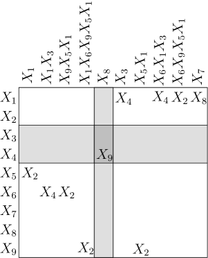
Figure 3: Relation $\mathcal{R}$ for the grammar presented in Figure 1. The highlighted ranges correspond to the result of searching for $b\cdot ar$, where the single primary occurrence corresponds to $X_{9}$.

6.2 Tracking Secondary Occurrences through the Grammar Tree

The remaining problem is how to track all the secondary occurrences triggered by a primary occurrence, and how to report the positions where these occur in $T$. Given a primary occurrence for partition $P=P_{1}\cdot P_{2}$ located at $v=\mathit{node}_{\mathcal{T}_{\mathcal{G}}}(p)$, we obtain the starting position of $P$ in $T$ by moving towards the root while keeping count of the offset between the beginning of the current node and the occurrence of $P$. Initially, for node $v$ itself, this is $l=-|P_{1}|$. Now, while $v$ is not the root, we set $l\leftarrow l+\mathit{select}_{1}(L,\mathit{leafrank}_{\mathcal{T}_{\mathcal{G}}}(v)+1)-\mathit{select}_{1}(L,\mathit{leafrank}_{\mathcal{T}_{\mathcal{G}}}(\mathit{parent}_{\mathcal{T}_{\mathcal{G}}}(v))+1)$, and $v\leftarrow\mathit{parent}_{\mathcal{T}_{\mathcal{G}}}(v)$. When we reach the root, the occurrence of $P$ starts at $l$.

It seems that we are doing this $h$ times in the worst case, since we need to track the occurrence up to the root. In fact we might do so for some symbols, but the total cost is amortized. Every time we move from $v$ to $u=\mathit{parent}_{\mathcal{T}_{\mathcal{G}}}(v)$, we know that $X[u]$ appears at least once more in the tree. This is because our preprocessing (Section  3) forces rules to appear at least twice or be removed. Thus $u$ defines $X[u]$, but there are one or more leaves labeled $X[u]$, and we have to report the occurrences of $P$ inside them all. For this sake we carry out $\mathit{select}_{X[u]}(X,i)$ for $i=2,3\ldots$ until spotting all those occurrences (where $P$ occurs with the current offset $l$). We recursively track them to the root of $\mathcal{T}_{\mathcal{G}}$ to find their absolute position in $T$, and recursively find the other occurrences of all their ancestor nodes. The overall cost amortizes to $O(1)$ steps per occurrence reported, as we can charge the cost of moving from $v$ to $u$ to the other occurrence of $u$. If we report $occ$ secondary occurrences we carry out $O(occ)$ steps, each costing $O(\lg\lg g)$ time.

7 The Resulting Index

By adding up the space of Lemma 1 with that of the labeled binary relation, and adding up the costs, we have our central result, Theorem 1.1, where for simplicity we have replaced the cost per occurrence of $1/\epsilon+\log\log g+\log g/\log\log G$ by just $1/\epsilon+\log g/\log\log g$.

By using $\epsilon=\Theta(1)$ and $\epsilon=1/\lg\lg n$, we obtain two simpler results.

Corollary 2

Let a sequence $T[1..n]$ be represented by a context-free grammar with $g$ symbols and size $G$. Then, for any constant $0<\epsilon\leq 1$, there exists a data structure using at most $G\lg n+2G\lg g+\epsilon\,g\lg g+o(G\lg g)+O(G)$ bits that finds the $occ$ occurrences of any pattern $P[1..m]$ in $T$ in time $O(m^{2}\lg\lg n+(m+occ)\lg g/\lg\lg g)$.

Corollary 3

Let a sequence $T[1..n]$ be represented by a context-free grammar with $g$ symbols and size $G$. Then, there exists a data structure using at most $G\lg n+2G\lg g+o(G\lg g)+O(G)$ bits that finds the $occ$ occurrences of any pattern $P[1..m]$ in $T$ in time $O((m\lg\lg n)^{2}+(m+occ)\lg g/\lg\lg g)$.

Finally, by using a larger geometric structure [CLP11] for the binary relation, and letting other structures use $O(G\lg n)$ bits, we obtain a somewhat faster structure, Corollary 1.

8 Implementation and Experiments

8.1 Implementation

We implemented our grammar-based self-index on top of the library SDSL (Succinct Data Structures Library), which is implemented in C++11 and contains efficient implementations of several succinct data structures.

To generate the grammar we use the RePair algorithm [LM00], in particular Navarro’s implementation. RePair produces a binary grammar (i.e., all the rules have 2 symbols in their right-hand side) plus a long initial rule. We then postprocess the resulting grammar as required for our index, see Section 3.

In repetitive collections it holds that $g\leq G\ll n$; we also expect that $\sigma\ll g$ for large texts. It follows that bitmaps $Y$ (of length $g$ and with $\sigma$ 1s) and $L$ (of length $n$ and with less than $G$ 1s) are sparse. We then represent them using the class sd_vector from SDSL.

In the compressed grammar representation we use a permutation $\pi$ to find the node that defines a rule. We use the class inv_permutation_support<$t$> of SDSL, which gives access to the inverse permutation in at most $t$ steps, and fix $t$ to 32. We also use this structure for representing the labels of the tries $T_{S}$ in the optimal prefix/suffix extraction.

To support operations on the sequence of non-primary nodes, $X^{\prime}$ is represented using the structure of Golynski et al. [GMR06] (wt_gmr in SDSL), because its alphabet is large and the sequence is almost incompressible.

Our grid representation is the same structure used in the implementation of Claude and Navarro [CN10] for labeled binary relations.

The topology of the grammar tree and of the sampled Patricia tries is represented with a variant of balanced FF (Section 2.3) called DFUDS [BDM⁺05], which is faster in practice for moving towards children. The trees $T_{S}$, instead, are represented using FF [NS14], which is more efficient for level ancestor queries. Both are implemented over the parentheses support of SDSL (bp_support_sada).

We test four versions of our index, called g-index in the experiments. The variants whose name continue with binary_search use plain binary search on the rules prefixes/suffixes in order to find the row and column intervals on the grid. The variants whose name instead continue with patricia_tree speed up this process using a sampled Patricia tree, which takes one string every 4, 8, 16, 32, and 64 positions. On the other hand, the variants suffixed trie use the structure of Gasieniec et al. [GKPS05] (Section 5.3) to extract rule prefixes/suffixes in optimal time, whereas the variants suffixed notrie omit this structure and extract the text from the rules in recursive form. Finally, the term gram indicates that we add a short $q$-gram ($q=2,4,6,8,10,12$) with the prefix and suffix of the expansion of each nonterminal [CFMPN16], to speed up extraction during binary searches. The strings are stored in a dictionary compressed with Huffman and Front Coding. Since the $q$-grams are limited, the binary search must be completed, either using plain decompression of nonterminals (suffix dfs), the real-time prefix extraction (suffix trie), or plain decompression speeded up by the same $q$-grams of the nonterminals we find in the way (suffix smp).

Our implementation is available at https://github.com/apachecom/grammar_improved_index/.

8.2 Experimental Setup

The experimental evaluation was carried out using the environment provided in Pizza&Chili (http://pizzachili.dcc.uchile.cl). We compared our implementation with the available indexes in the state of the art that are most faithful with respect to different compressibility measures:

slp-index​​

is the only previous implementation of a grammar-based index [CN10], using $O(G\log n)$ bits like ours. It does not guarantee, however, logarithmic locating time per occurrence. It uses the same RePair algorithm we use to build the index (a construction over the heuristically balanced version of RePair is called slp-index-bal). In its optimized version [CFMPN16], it speeds up the binary searches by storing the $q$-gram prefixes of the strings expanded by each nonterminal, as we use in the gram variant of q-index, yet here the best values are $q=4,8,16$.

lz-index​​

is the only implementation of a Lempel-Ziv based index [KN13] that guarantees $O(z\log n)$ bits of space on a Lempel-Ziv parse of $z$ phrases. We also use its optimized implementation [CFMPN16], which was shown to outperform slp-index both in space and time.

r-index​​

is the only implementation of a classical self-index (i.e., suffix-array based) using $O(r\log n)$ bits, where $r$ is the number of runs in the Burrows-Wheeler Transform of the text [GNP18].

We use six real repetitive collections from a repetitive corpus. Three of these collections contain DNA sequences extracted from differents sources: para and cere are extracted from the Saccharomyces Genome Resequencing Project, whereas influenza is formed by DNA sequences of H. Influenzae taken from the National Center for Biotechnology Information (NCBI). Collection einstein.en is formed by all version of the articles in English of Albert Einstein taken from Wikipedia. Collections kernel and coreutils are formed by all versions 5.x of the Coreutils package and all 1.0.x and 1.1.x versions of the Linux Kernel, respectively. Table 1 lists their main characteristics.

Collection	$n$	$\sigma$	$z$	$r$	$G$ – repair	$G$ – proc
para	429,265,758	5	2,332,908	15,636,740	7,338,520	5,344,480
cere	461,286,644	5	1,700,859	11,574,641	5,780,080	4,069,450
influenza	154,808,555	15	770,253	3,022,822	2,174,650	1,957,370
einstein.en	467,626,544	139	91,036	290,239	263,962	212,903
kernel	257,961,616	162	794,290	2,791,368	2,185,860	1,374,650
coreutils	205,281,778	235	1,446,891	4,684,465	3,798,100	2,409,460

Table 1: Main characteristics of the collections: $n$ (size in bytes), $\sigma$ (alphabet size), $z$ (number of Lempel-Ziv phrases), $r$ (number of runs in the BWT), and $G$ – repair and $G$ – proc (size of the RePair grammar before and after applying the transformations of Section 3, respectively).

Our times per occurrence are the average over 1000 patterns of length 10 extracted at random from each collection. Our extraction times average over 1000 queries at random text positions.

8.3 Locate Time

Figure 4 shows the space-time tradeoffs obtained for locating patterns of length 10 over all the indexes and parameter values on all the collections. We first discuss the results on our index and then compare it with the others.

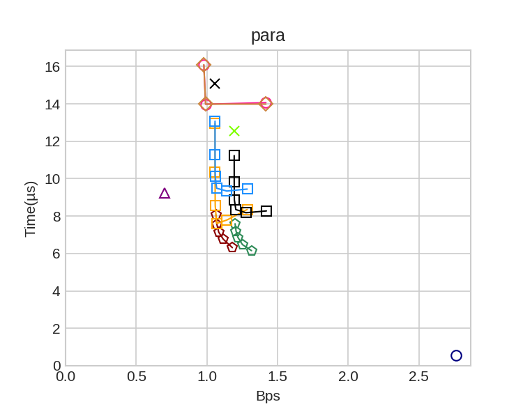
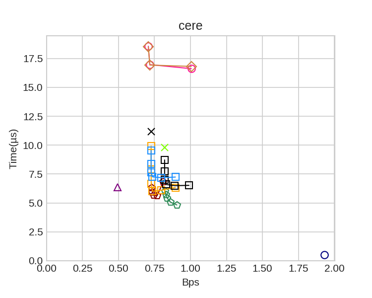
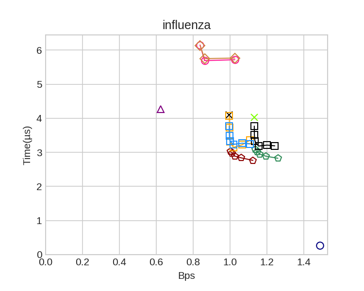
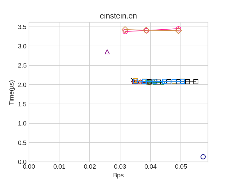
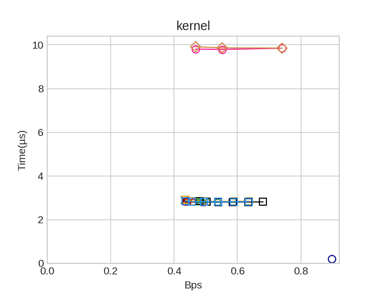
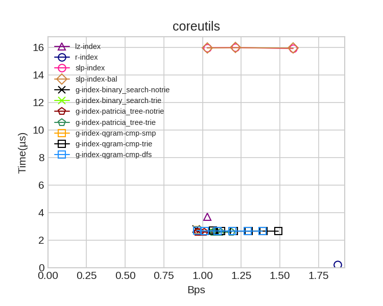
Figure 4: Time-space tradeoffs for locating on different collections and indexes. The time is given in microseconds per occurrence and the space in bits per symbol (bps).

In all cases, the use of Patricia trees with a sufficiently sparse sampling rate can reach essentially the same space of the plain binary-search versions. Even with the sparsest sampling rate (1 out of 64), the Patricia trees sharply outperform the binary searches on the DNA alphabets, while making no difference on the others. The rule samplings of the qgram versions also outperform binary searches on DNA alphabets without increasing the space, reaching the sweet point at value 8. Nevertheless, the Patricia trees make better use of the space.

On the other hand, the use of the tries $T_{S}$ slightly increases the space while not providing a noticeable improvement in time (the exception is on the binary-search versions of para, but these lose anyway to the versions using Patricia trees). As a result, we take g-index-patricia_tree-notrie as the most convenient version of our implementation, and we call it simply g-index henceforth.

The use of denser samplings yields an interesting space-time tradeoff for g-index on DNA, which dominates a significant part of the Pareto curve. On the other texts, it is better to use it with the sparsest sampling (or with plain binary search), which dominates all the other alternatives on kernel and coreutils. With the sparsest sampling, g-index uses almost the same space of the previous grammar-based index, slp-index, except on influenza, where g-index is 20% larger. In exchange, g-index is up to 5 times faster than slp-index. There are almost no differences between slp-index and slp-index-bal, which confirms that the grammar height does not affect extraction time in practice.

Index lz-index outperforms slp-index in both space and time, as in previous work [CFMPN16]. While losing to lz-index in space is expected because $z\leq G$ always holds, grammars allow for better methods to access the text. The index slp-index was, however, unable to take advantage of those methods to outperform lz-index in time. Now our g-index does offer a space-time tradeoff, using more space than lz-index, but in exchange being faster; sometimes lz-index is dominated in space and time. With sampling value 8, g-index is 50%–65% larger than lz-index, but 30%–40% faster on DNA texts. With sampling value 64, g-index is from 10% smaller to 25% larger than lz-index and 20%–40% faster than it.

Finally, r-index is way faster than the others, but also way larger (2–5 times larger than lz-index).

Figure 5 shows how the locate time evolves with the pattern length $m$ on einstein.en. We still include the different variants of our index in this plot (the numbers in brackets are the sample values), and consider pattern lengths 5, 10, 20, 30, 40, and 50.

The left plot shows that, while g-index is way faster than slp-index and lz-index on this text for small $m$, all the g-index variants slow down as $m$ increases, eventually losing to lz-index for long enough patterns. The most important lengths, however, where a large number of occurrences are found, are the short ones. The total query times are much less significant for long patterns, as shown on the right plot.

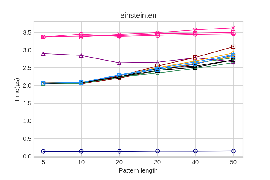
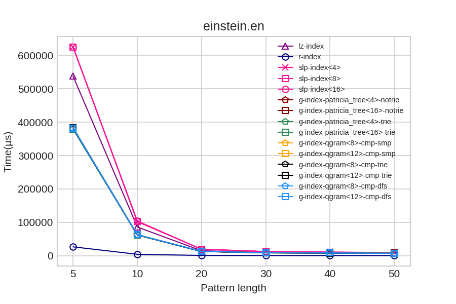
Figure 5: Locating time for increasing pattern lenghts on einstein.en. The time is given in microseconds per occurrence on the left, and per pattern symbol on the right. Only some representative indexes are shown on the right plot.

8.4 Extraction Time

Figure 6 shows the time per extracted symbol of the different indexes and collections, when extracting 10 consecutive text symbols. The r-index is excluded because it does not support this operation. Note that the extraction in our g-index is independent of whether or not we use binary search or Patricia trees. The variant that continues with binary_search descends from the root symbol, binary searching the children, to reach the desired substring to extract. Instead, the variant that continues with rank_phrases uses $\mathit{rank}$ on the bitmap $L$ (Section 5.2), so as to find faster the phrases to be expanded. The suffixes trie and notrie refer again to using or not the structure for extracting prefixes and suffixes in linear time (for the phrases that are not completely contained in the area to extract). Finally, if qgram follows g-index, we use the $q$-grams to speed up extraction, with lengths $2,4,6,8$.

As it can be seen, the best g-index variant, both in space and time, is usually g-index-rank_phrases-notrie. It is also apparent that lz-index excells in extraction, being 3–5 times faster than every g-index variant (except on einstein.en, the most repetitive collection, where the $\bar{h}$ value of the Lempel-Ziv parsing is very high). On the other hand, our best g-index variant outperforms slp-index in time by 20%–100% within similar space. The exceptions are influenza and einstein.en, where slp-index is 10%–30% faster.

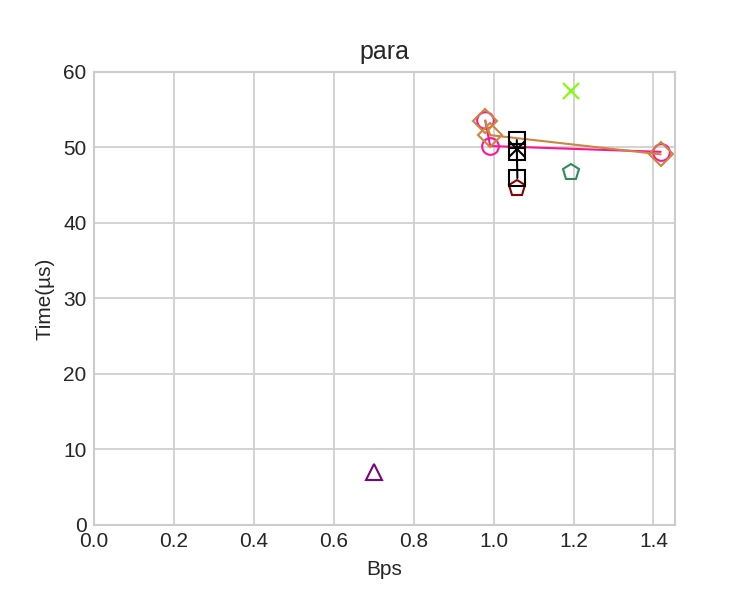
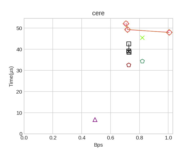
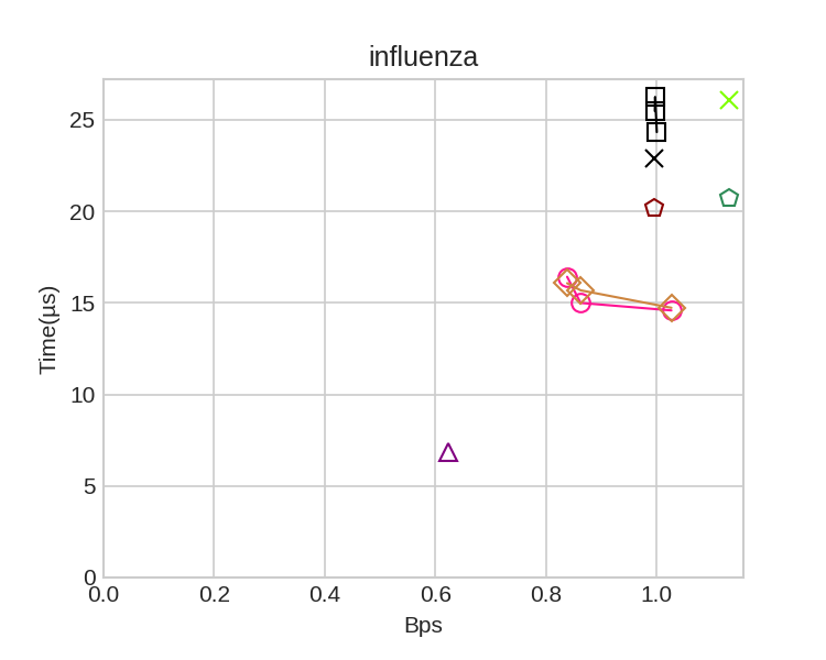
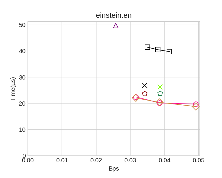
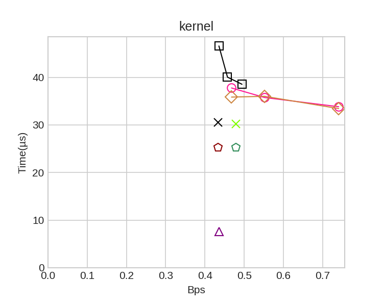
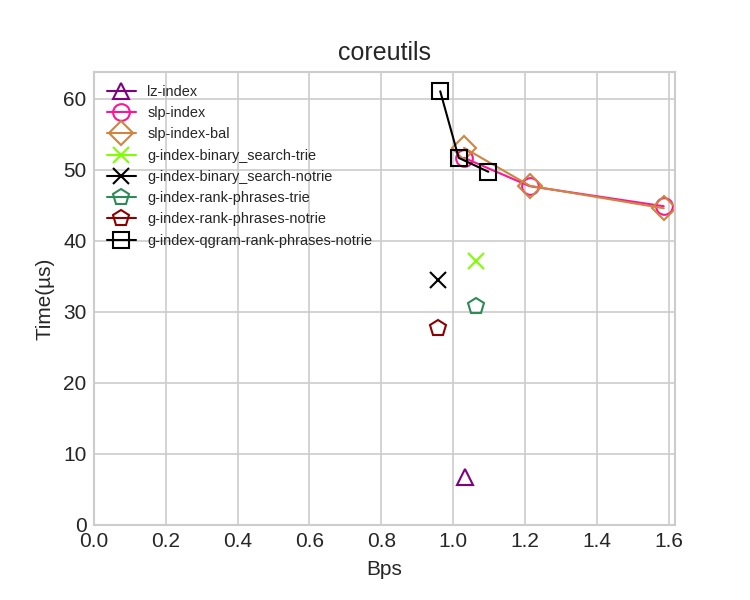
Figure 6: Time-space tradeoffs for extracting on different collections and indexes. The time is given in microseconds per extracted symbol and the space in bits per symbol (bps).

9 Conclusions

We have presented the first compressed text index based on arbitrary context-free grammars whose time per retrieved occurrence is logarithmic, independently of the grammar height. Given a text $T[1..n]$ represented by a grammar of size $G$, our index uses $O(G\log n)$ bits of space and returns the $occ$ occurrences of a pattern $P[1..m]$ in time $O((m^{2}+occ)\log G)$. We implemented our index and compared it with various alternatives in the literature, showing that it is practical and offers relevant space/time tradeoffs.

The most interesting open theoretical question is whether it is possible to obtain $O(G\log g)$ bits, as grammar-based compressors could reach, instead of $O(G\log n)$, since in some text families we have $g\leq G=O(\log n)$. This term owes to storing the lengths of the expansions of the nonterminals in bitmap $L$. We tried storing these lengths in the nonterminals, instead, and sampling the nonterminals that would store lengths. Finding a suitable sampling on the grammar DAG, however, is related to finding minimum cuts in graphs [AHK04], which is not easy.

With respect to practical results, an interesting research direction would be to obtain practical implementations of recent proposals that reduce the $O(m^{2})$ term in the search complexity [GGK⁺14, BEGV18, CE18]. Some of those methods, however, have a penalty factor of $O(\log\log z)$ or $O(\log(n/z))$ in the space, which is far from negligible, and thus they are unlikely to be competitive in space. The index of Christiansen and Ettienne [CE18], on the other hand, builds on a grammar and looks more promising. They manage to ensure that $P$ needs be cut into only $O(\log m)$ places to spot all the primary occurrences, which reduces the $O(m^{2})$ term to $O(m\log m)$. For this to hold, however, the grammar must be of a special type called locally-consistent. In our experience, RePair outperforms in space, by a wide margin, all the other grammar construction algorithms, including those that offer guarantees of the form $G=O(z\log(n/z))$. It is therefore unclear which is the price to pay in space in order to use a specific type of grammar.

References

- [AB92] A. Amir and G. Benson. Efficient two-dimensional compressed matching. In Proc. 2nd Data Compression Conference (DCC), pages 279–288, 1992.
- [AHK04] S. Arora, E. Hazan, and S. Kale. approximation to SPARSEST CUT in time. In Proc. 45th Annual Symposium on Foundations of Computer Science (FOCS), pages 238–247, 2004.
- [ANS12] D. Arroyuelo, G. Navarro, and K. Sadakane. Stronger Lempel-Ziv based compressed text indexing. Algorithmica, 62(1):54–101, 2012.
- [BCG+15] D. Belazzougui, F. Cunial, T. Gagie, N. Prezza, and M. Raffinot. Composite repetition-aware data structures. In Proc. 26th Annual Symposium on Combinatorial Pattern Matching (CPM), LNCS 9133, pages 26–39, 2015.
- [BCN13] J. Barbay, F. Claude, and G. Navarro. Compact binary relation representations with rich functionality. Information and Computation, 232:19–37, 2013.
- [BDM+05] D. Benoit, E. Demaine, J. I. Munro, R. Raman, V. Raman, and S. Srinivasa Rao. Representing trees of higher degree. Algorithmica, 43(4):275–292, 2005.
- [BEGV18] P. Bille, M. B. Ettienne, I. L. Gørtz, and H. W. Vildhøj. Time-space trade-offs for Lempel-Ziv compressed indexing. Theoretical Computer Science, 713:66–77, 2018.
- [BGG+14] D. Belazzougui, T. Gagie, S. Gog, G. Manzini, and J. Sirén. Relative FM-indexes. In Proc. 21st International Symposium on String Processing and Information Retrieval (SPIRE), LNCS 8799, pages 52–64, 2014.
- [BLR+15] P. Bille, G. M. Landau, R. Raman, K. Sadakane, S. S. Rao, and O. Weimann. Random access to grammar-compressed strings and trees. SIAM Journal on Computing, 44(3):513–539, 2015.
- [BN15] D. Belazzougui and G. Navarro. Optimal lower and upper bounds for representing sequences. ACM Transactions on Algorithms, 11(4):article 31, 2015.
- [BPT15] D. Belazzougui, S. J. Puglisi, and Y. Tabei. Access, rank, select in grammar-compressed strings. In Proc. 23rd Annual European Symposium on Algorithms (ESA), LNCS 9294, pages 142–154, 2015.
- [CE18] A. R. Christiansen and M. B. Ettienne. Compressed indexing with signature grammars. In Proc. 13th Latin American Symposium on Theoretical Informatics (LATIN), pages 331–345, 2018.
- [CFMPN10] F. Claude, A. Fariña, M. Martínez-Prieto, and G. Navarro. Compressed -gram indexing for highly repetitive biological sequences. In Proc. 10th IEEE Conference on Bioinformatics and Bioengineering (BIBE), 2010.
- [CFMPN16] F. Claude, A. Fariña, M. Martínez-Prieto, and G. Navarro. Universal indexes for highly repetitive document collections. Information Systems, 61:1–23, 2016.
- [Cla96] D. Clark. Compact Pat Trees. PhD thesis, University of Waterloo, 1996.
- [CLL+05] M. Charikar, E. Lehman, D. Liu, R. Panigrahy, M. Prabhakaran, A. Sahai, and A. Shelat. The smallest grammar problem. IEEE Transactions on Information Theory, 51(7):2554–2576, 2005.
- [CLP11] T. M. Chan, K. G. Larsen, and M. Pătraşcu. Orthogonal range searching on the RAM, revisited. In Proc. 27th ACM Symposium on Computational Geometry (SoCG), pages 1–10, 2011.
- [CN10] F. Claude and G. Navarro. Self-indexed grammar-based compression. Fundamenta Informaticae, 111(3):313–337, 2010.
- [CN12] F. Claude and G. Navarro. Improved grammar-based compressed indexes. In Proc. 19th International Symposium on String Processing and Information Retrieval (SPIRE), LNCS 7608, pages 180–192, 2012.
- [CRA76] C. Cook, A. Rosenfeld, and A. Aronson. Grammatical inference by hill climbing. Information Science, 10:59––80, 1976.
- [DJSS14] H. H. Do, J. Jansson, K. Sadakane, and W.-K. Sung. Fast relative Lempel-Ziv self-index for similar sequences. Theoretical Computer Science, 532:14–30, 2014.
- [Eli74] P. Elias. Efficient storage and retrieval by content and address of static files. Journal of the ACM, 21:246–260, 1974.
- [Fan71] R. Fano. On the number of bits required to implement an associative memory. Memo 61, Computer Structures Group, Project MAC, Massachusetts, 1971.
- [FM05] P. Ferragina and G. Manzini. Indexing compressed texts. Journal of the ACM, 52(4):552–581, 2005.
- [GGK+12] T. Gagie, P. Gawrychowski, J. Kärkkäinen, Y. Nekrich, and S. J. Puglisi. A faster grammar-based self-index. In Proc. 6th International Conference on Language and Automata Theory and Applications (LATA), LNCS 7183, pages 240–251, 2012.
- [GGK+14] T. Gagie, P. Gawrychowski, J. Kärkkäinen, Y. Nekrich, and S. J. Puglisi. LZ77-based self-indexing with faster pattern matching. In Proc. 11th Latin American Theoretical Informatics Symposium (LATIN), LNCS 8392, pages 731–742, 2014.
- [GKPS05] L. Gasieniec, R. Kolpakov, I. Potapov, and P. Sant. Real-time traversal in grammar-based compressed files. In Proc. 15th Data Compression Conference (DCC), page 458, 2005.
- [GMR06] A. Golynski, J. I. Munro, and S. Rao. Rank/select operations on large alphabets: a tool for text indexing. In Proc. 17th Annual ACM-SIAM Symposium on Discrete Algorithms (SODA), pages 368–373, 2006.
- [GNP18] T. Gagie, G. Navarro, and N. Prezza. Optimal-time text indexing in BWT-runs bounded space. In Proc. 29th Annual ACM-SIAM Symposium on Discrete Algorithms (SODA), pages 1459–1477, 2018.
- [HLR16] D. Hucke, M. Lohrey, and C. P. Reh. The smallest grammar problem revisited. In Proc. 23rd International Symposium on String Processing and Information Retrieval, LNCS 9954, pages 35–49, 2016.
- [Jez15] A. Jez. Approximation of grammar-based compression via recompression. Theoretical Computer Science, 592:115–134, 2015.
- [Jez16] A. Jez. A really simple approximation of smallest grammar. Theoretical Computer Science, 616:141–150, 2016.
- [Kär99] J. Kärkkäinen. Repetition-Based Text Indexing. PhD thesis, U. Helsinki, Finland, 1999.
- [KMS+03] T. Kida, T. Matsumoto, Y. Shibata, M. Takeda, A. Shinohara, and S. Arikawa. Collage system: a unifying framework for compressed pattern matching. Theoretical Computer Science, 298(1):253–272, 2003.
- [KN13] S. Kreft and G. Navarro. On compressing and indexing repetitive sequences. Theoretical Computer Science, 483:115–133, 2013.
- [KY00] J. Kieffer and E.-H. Yang. Grammar-based codes: A new class of universal lossless source codes. IEEE Transactions on Information Theory, 46(3):737–754, 2000.
- [LM00] J. Larsson and A. Moffat. Off-line dictionary-based compression. Proc. IEEE, 88(11):1722–1732, 2000.
- [LZ76] A. Lempel and J. Ziv. On the complexity of finite sequences. IEEE Transactions on Information Theory, 22(1):75–81, 1976.
- [MNSV10] V. Mäkinen, G. Navarro, J. Sirén, and N. Välimäki. Storage and retrieval of highly repetitive sequence collections. Journal of Computational Biology, 17(3):281–308, 2010.
- [Mor68] D. Morrison. PATRICIA – practical algorithm to retrieve information coded in alphanumeric. Journal of the ACM, 15(4):514–534, 1968.
- [MRRR12] J. I. Munro, R. Raman, V. Raman, and S. S. Rao. Succinct representations of permutations and functions. Theoretical Computer Science, 438:74–88, 2012.
- [Nav12] G. Navarro. Indexing highly repetitive collections. In Proc. 23rd International Workshop on Combinatorial Algorithms (IWOCA), LNCS 7643, pages 274–279, 2012.
- [NM07] G. Navarro and V. Mäkinen. Compressed full-text indexes. ACM Computing Surveys, 39(1):article 2, 2007.
- [NMWM94] C. Nevill-Manning, I. Witten, and D. Maulsby. Compression by induction of hierarchical grammars. In Proc. 4th Data Compression Conference (DCC), pages 244–253, 1994.
- [NP19] G. Navarro and N. Prezza. Universal compressed text indexing. Theoretical Computer Science, 762:41–50, 2019.
- [NPC+13] J. C. Na, H. Park, M. Crochemore, J. Holub, C. S. Iliopoulos, L. Mouchard, and K. Park. Suffix tree of alignment: An efficient index for similar data. In Proc. 24th International Workshop on Combinatorial Algorithms (IWOCA), LNCS 8288, pages 337–348, 2013.
- [NPL+13] J. C. Na, H. Park, S. Lee, M. Hong, T. Lecroq, L. Mouchard, and K. Park. Suffix array of alignment: A practical index for similar data. In Proc. 20th International Symposium on String Processing and Information Retrieval (SPIRE), LNCS 8214, pages 243–254, 2013.
- [NS14] G. Navarro and K. Sadakane. Fully-functional static and dynamic succinct trees. ACM Transactions on Algorithms, 10(3):article 16, 2014.
- [RO08] L. Russo and A. Oliveira. A compressed self-index using a Ziv-Lempel dictionary. Information Retrieval, 11(4):359–388, 2008.
- [RRR07] R. Raman, V. Raman, and S. S. Rao. Succinct indexable dictionaries with applications to encoding k-ary trees, prefix sums and multisets. ACM Transactions on Algorithms, 3(4):article 43, 2007.
- [Ryt03] W. Rytter. Application of Lempel-Ziv factorization to the approximation of grammar-based compression. Theoretical Computer Science, 302(1-3):211–222, 2003.
- [SS82] J. A. Storer and T. G. Szymanski. Data compression via textual substitution. Journal of the ACM, 29(4):928–951, 1982.
- [Sto77] J. A. Storer. NP-completeness results concerning data compression. Technical Report 234, Department of Electrical Engineering and Computer Science, Princeton University, 1977.
- [VY13] E. Verbin and W. Yu. Data structure lower bounds on random access to grammar-compressed strings. In Proc. 24th Annual Symposium on Combinatorial Pattern Matching (CPM), LNCS 7922, pages 247–258, 2013.
- [ZL78] J. Ziv and A. Lempel. Compression of individual sequences via variable length coding. IEEE Transactions on Information Theory, 24(5):530–536, 1978.