The high-temperature rotation-vibration spectrum and rotational clustering of silylene (SiH₂)

Abstract

A rotation-vibration line list for the electronic ground state ($\tilde{X}^{1}A_{1}$) of SiH₂ is presented. The line list, named CATS, is suitable for temperatures up to 2000 K and covers the wavenumber range 0–10 000 cm^-1 (wavelengths $>1.0$ $\mu$m) for states with rotational excitation up to $J=52$. Over 310 million transitions between 593 804 energy levels have been computed variationally with a new empirically refined potential energy surface, determined by refining to 75 empirical term values with $J\leq 5$ and a newly computed high-level ab initio dipole moment surface. This is the first, comprehensive high-temperature line list to be reported for SiH₂ and it is expected to aid the study of silylene in plasma physics, industrial processes and possible astronomical detection. Furthermore, we investigate the phenomenon of rotational energy level clustering in the spectrum of SiH₂. The CATS line list is available from the ExoMol database (www.exomol.com) and the CDS database.

1 Introduction

The spectrum of SiH₂, known as silylene or silicon dihydride, was first observed in the late 1960s [1] and, since then, numerous experimental and theoretical studies have followed (see Ref. [2] and references within). Its importance in silicon chemistry is largely owing to it being an intermediate in many chemical reactions involving silane (SiH₄). For example, the formation of SiH₂ is used to monitor the decomposition of SiH₄ into silylene and hydrogen; and the loss of SiH₂ can be used to track the formation of disilane (Si₂H₆) [3, 4, 5]. Given the widespread use of silane plasmas in industry, detailed spectroscopic information on SiH₂ can significantly help the detection and monitoring of certain processes, such as the deposition of hydrogenated amorphous silicon (a-Si:H) films, the chemistry of which is not fully understood [6]. Silylene is yet to be conclusively detected astronomically with unsuccessful searches in the circumstellar envelope of the carbon star IRC+10216 [7, 8], despite speculation of its presence in these environments [9].

Theoretical work on SiH₂ has primarily focused on ab initio predictions of the electronic state ordering relative to the isovalent methylene (CH₂), which interestingly has a triplet ground state (see Refs. [10, 11] and references within). More closely related to this study are the full-dimensional variational calculations of the ro-vibrational and ro-vibronic spectra of the ground and excited singlet states, $\tilde{X}^{1}A_{1}$, $\tilde{A}^{1}B_{1}$ and $\tilde{B}^{1}A_{1}$ [12, 13, 14]. Nowadays, variational approaches are more robust and can offer high-accuracy predictions of line positions and intensities over extended wavenumber ranges, capable of supporting high-resolution spectroscopic measurements [15]. In particular, they have found widespread application in exoplanetary science through the ExoMol database [16, 17], which provides molecular line lists on a large variety of small molecules relevant to the atmospheric characterization of exoplanets and other hot bodies. In particular the ExoMol database already contains line lists for a number of silicon-bearing molecules: SiH₄ [18], SiH [19], SiO [20] and SiS [21]. It is within the ExoMol computational framework [22] that we treat silylene.

In this paper, we present a comprehensive molecular line list for the ground electronic state $\tilde{X}^{1}A_{1}$ of SiH₂. The line list, named CATS, has been computed using robust first-principles methodologies with a degree of empirical tuning to the available spectroscopic data, namely the refinement of a newly computed high-level ab initio potential energy surface (PES) to experimentally determined ro-vibrational term values. The CATS line list is applicable for temperatures up to $T=2000$ K and contains over 254 million transitions between states with rotational excitation up to $J=51$.

Interestingly, triatomic symmetrical hydrides of the form XH₂ with a heavy central nuclei X and an interbond angle close to 90^∘ exhibit well separated, near-degenerate rotational energy level clusters at high rotational excitation [23]. This effect arises in local-mode molecules when the bonds are nearly orthogonal to each other such that the rotation of the molecule is not destabilized by Coriolis-type interactions with the vibrational modes. The new CATS line list is used to explore this phenomenon in SiH₂, which has an interbond angle $\alpha_{\rm e}=92.04^{\circ}$ [2] and is expected to form rotational cluster states at high rotational excitation.

The paper is structured as follows: In Sec. 2 we describe the theoretical approach including the construction of the PES and subsequent empirical refinement, the dipole moment surface (DMS) and the variational calculations used to produce the line list. In Sec. 3, the line list is presented and evaluated along with analysis of the temperature-dependent partition function. In Sec. 4, rotational energy level clustering in SiH₂ is investigated. Conclusions are offered in Sec. 5.

2 Theoretical approach

2.1 Potential Energy Surface

The initial ab initio PES was computed using the explicitly correlated coupled cluster method CCSD(T)-F12c [24] with the F12-optimized correlation consistent basis set, cc-pVQZ-F12 [25] in the frozen core approximation. Calculations employed the diagonal fixed amplitude ansatz 3C(FIX) [26] and a Slater geminal exponent value of $\beta=1.0$ $a_{0}^{-1}$ [27]. The auxiliary basis sets were chosen to be the resolution of the identity OptRI [28] basis and the cc-pV5Z/JKFIT [29] and aug-cc-pwCV5Z/MP2FIT [30] basis sets for density fitting. MOLPRO2015 [31] was used for all electronic structure calculations. The PES was computed on a uniformly-spaced grid of 1898 nuclear geometries with energies up to $hc\cdot 19\,300$ cm^-1 ($h$ is the Planck constant and $c$ is the speed of light). The grid was built in terms of three internal coordinates: the two Si–H bond lengths $1.2\leq r_{\rm SiH_{1}},r_{\rm SiH_{2}}\leq 2.0$ Å and the interbond angle $30\leq\alpha({\rm H_{1}SiH_{2}})\leq 160^{\circ}$.

The three coordinates of the PES were chosen to be,

$$y_{1} = 1-\exp\left(-b(r_{1}-r_{\rm e})\right),$$ (1)

$$y_{2} = 1-\exp\left(-b(r_{2}-r_{\rm e})\right),$$ (2)

$$y_{3} = \cos\alpha-\cos\alpha_{\rm e},$$ (3)

where $r_{1}$ and $r_{2}$ are the bond lengths Si-H₁ and Si-H₂, respectively, $b$ is the Morse parameter, $\alpha$ is the interbond angle $\angle$(H-Si-H), and $r_{\rm e}$ and $\alpha_{\rm e}$ are the corresponding equilibrium parameters. The PES was represented using the analytical function [32],

$$V=V_{0}+V_{\rm HH},$$ (4)

where

$$V_{0}=\sum_{0\leq i+j+k\leq 6}f_{ijk}y_{1}^{i}y_{2}^{j}y_{3}^{k},$$ (5)

and

$$V_{\rm HH}=B_{1}\exp(-g_{1}r_{\rm HH})+B_{2}\exp(-g_{2}r_{\rm HH}^{2}).$$ (6)

The $f_{ijk}$ expansion parameters obey the symmetric relation $f_{ijk}=f_{jik}$ owing to the identical properties of the hydrogen atoms 1 and 2. The distance between the hydrogen nuclei

$$r_{\rm HH}=\sqrt{r_{1}^{2}+r_{2}^{2}-2r_{1}r_{2}\cos\alpha},$$ (7)

and the numerical parameters $B_{1}$, $B_{2}$, $g_{1}$ and $g_{2}$ are taken as in Ref. [32] (see supplementary material for values). The contribution $V_{\rm HH}$ is to prevent holes appearing in the PES at geometries where $r_{\rm HH}$ is small. The ab initio data was weighted with factors of the form [33]

$$w_{i}=\left(\frac{\tanh\left[-0.0008\times(\tilde{E}_{i}-12{\,}000)\right]+1.002002002}{2.002002002}\right).$$ (8)

Watson’s robust fitting scheme [34] was also utilized to reduce the weights of outliers and improve the description at lower energies. A total of 53 parameters were varied (46 expansion parameters + 2 equilibrium parameters + 1 Morse parameter + 4 damping parameters) in a least-squares fitting to the ab initio data which were reproduced with a weighted root-mean-square (rms) error of 0.0048 cm^-1.

2.2 Dipole Moment Surface

To represent the instantaneous dipole moment vector $\bm{\mu}$ of SiH₂, we employed the so-called $pq$ axis system [35]. The $p$ and $q$ axes were defined in the plane of the three nuclei with origin at the Si atom. The $q$ axis bisects the interbond angle and the $p$ axis lies perpendicular to the $q$ axis. In electronic structure calculations, an external electric field with components $\pm 0.005$ a.u. was applied along each axis and the respective dipole moment component $\mu_{p}$ and $\mu_{q}$ determined using central finite differences. Calculations were at the same level of theory as the PES, namely CCSD(T)-F12c/cc-pVQZ-F12 and used the same grid of 1898 nuclear geometries.

In order to represent the two dipole components analytically the following expansions were used [36] (see also Ref. [37]),

$$\mu^{(q)} = \sin\alpha\sum_{i+j+k\leq 5}F^{(q)}_{ijk}\xi_{1}^{i}\xi_{2}^{j}\xi_{3}^{k},$$ (9)

$$\mu^{(p)} = \sum_{i+j+k\leq 5}F^{(p)}_{ijk}\xi_{1}^{i}\xi_{2}^{j}\xi_{3}^{k},$$ (10)

where the coordinates

$$\xi_{1} = r_{1}-r_{\rm e},$$ (11)

$$\xi_{2} = r_{2}-r_{\rm e},$$ (12)

$$\xi_{3} = \cos\alpha-\cos\alpha_{\rm e}.$$ (13)

The dipole expansion parameters $F^{(q)}_{ijk}$ and $F^{(p)}_{ijk}$ are subject to the conditions that the function $\mu^{(q)}$ is unchanged under the interchange of the identical protons, whereas the function $\mu^{(p)}$ is antisymmetric under this operation. The same analytic representation of the DMS was first used for CH₂ [35] and also previously for SiH₂ [13].

The dipole expansion parameters were determined through a least-squares fitting to the ab initio data. The same weight factors as given in Eq. (8) were used along with Watson’s robust fitting scheme and the equilibrium parameters fixed to $r_{\rm e}=1.514$ Å and $\alpha_{\rm e}=92.0^{\circ}$. The $\mu_{p}$ component required 20 parameters (including the 2 equilibrium parameters) and reproduced the ab initio data with a weighted rms error of $1.5\times 10^{-4}$ D with the $\mu_{q}$ component using 26 parameters (including the 2 equilibrium parameters) giving a weighted rms error of $1\times 10^{-3}$ D. The DMSs of SiH₂ are provided in the supplementary material. Our ab initio dipole moment at the equilibrium (0.066 D) is in a good agreement with the ab initio equilibrium dipole moment reported by Gabriel et al. [12] (0.075 D) and slightly smaller than the equilibrium dipole moment from Ref. [13] (0.14 D).

2.3 Variational calculations

Variational calculations were performed with the nuclear motion program TROVE [38] and details of its methodology are discussed extensively elsewhere [38, 39, 40, 22]. Here, we summarise the main calculation steps.

The TROVE kinetic energy operator was constructed as a sixth-order Taylor expansion around the SiH₂ equilibrium geometry in terms of the following linearized coordinates,

$$\chi_{1}^{\rm lin} = r_{1}^{\rm lin}-r_{\rm e},$$ (14)

$$\chi_{2}^{\rm lin} = r_{2}^{\rm lin}-r_{\rm e},$$ (15)

$$\chi_{3}^{\rm lin} = \alpha^{\rm lin}-\alpha_{\rm e}.$$ (16)

where $r_{i}^{\rm lin}$ and $\alpha^{\rm lin}$ are the linearized versions of $r_{i}$ and $\alpha$, respectively (see Ref. [38]). The PES was also re-expanded to sixth-order in terms of the coordinates

$$\zeta_{1}^{\rm lin} = 1-\exp(-b(r_{1}^{\rm lin}-r_{\rm e})),$$ (17)

$$\zeta_{2}^{\rm lin} = 1-\exp(-b(r_{2}^{\rm lin}-r_{\rm e})),$$ (18)

$$\zeta_{3}^{\rm lin} = \alpha^{\rm lin}-\alpha_{\rm e}.$$ (19)

For the primitive basis set, TROVE uses 1D numerical basis functions $\phi_{n_{1}}(\chi_{1})$, $\phi_{n_{2}}(\chi_{2})$ and $\phi_{n_{3}}(\chi_{3})$ constructed with the Numerov-Cooley approach [41, 42]. The eigenfunctions of the 1D stretching and bending Hamiltonian operators $\hat{H}_{i}^{\rm(1D)}$ were obtained by freezing all other degrees of freedom at their equilibrium values. In order to improve the primitive basis set by making it more compact, a two-step contraction scheme is used. At step 1, the 1D basis functions are combined into two subgroups, one for the stretches

$$\phi^{\rm(2D)}_{n_{1},n_{2}}(\chi_{1},\chi_{2})=\phi_{n_{1}}(\chi_{1})\phi_{n_{2}}(\chi_{2}),$$ (20)

and the other for the bending mode,

$$\phi^{\rm(1D)}_{n_{3}}(\chi_{1})=\phi_{n_{3}}(\chi_{3})$$ (21)

and these are used to solve the respective reduced Hamiltonian operators (stretching $\hat{H}^{\rm(2D)}$ and bending $\hat{H}^{\rm(1D)}$). The reduced Hamiltonians are constructed by averaging the total vibrational Hamiltonian operator $\hat{H}^{(J=0)}$ over the other ground vibrational basis functions [43, 44]. The resulting eigenfunctions of the two reduced problems, $\psi^{\rm(2D)}_{\lambda_{1},\lambda_{2}}$ and $\psi^{\rm(1D)}_{\lambda_{3}}$, are contracted and classified according to the ${\mathcal{C}}_{2{\rm v}}$(M) symmetry group [45] using an optimized symmetrization procedure [40] to form a symmetry-adapted 3D vibrational basis set as a product $\psi^{\rm(2D)}_{\lambda_{1}\lambda_{2}}\psi^{\rm(1D)}_{\lambda_{3}}$. This vibrational basis set is then used for the $J=0$ eigenproblem at step 2, with the eigenfunctions contracted again and used to form the symmetry-adapted $J>0$ ro-vibrational basis set.

In steps 1 and 2 an additional basis set cut-off was applied based on the polyad number,

$$P=2(n_{1}+n_{2})+n_{3}\leq P_{\rm max}$$ (22)

which used the polyad cutoff $P_{\rm max}=24$. The maximal values of $n_{1},n_{2}$ and $n_{3}$ that define the size of the primitive basis set were 12, 12 and 24, respectively. The contracted $J=0$ basis set contained 192 and 143 basis functions with energies up to 16 000 cm^-1 for the $A_{1}$ and $B_{2}$ symmetries, respectively. For the rotational basis set, symmetrized spherical harmonics were used [40].

Line list calculations employed the empirically refined PES (discussed below) and ab initio DMS. All transitions and corresponding line strengths were computed for the 0–10 000 cm^-1 range with a lower state energy threshold of 10 000 cm^-1 and upper state threshold of 18 000 cm^-1. States were computed up to $J=60$ but only those below $J=51$ contributed to the line list with the $J>51$ energies lying above 10 000 cm^-1. The nuclear spin statistical weights of ²⁸Si¹H₂ are $g_{(\rm ns)}=\{1,1,3,3\}$ for states of symmetry $\{A_{1},A_{2},B_{1},B_{2}\}$, respectively. Atomic mass values were used for the TROVE calculations.

2.4 Potential energy surface refinement

To improve the accuracy of the computed line list the initial ab initio PES was empirically refined using an efficient least-squares fitting procedure [46] implemented in TROVE. Experimental term values up to $J=5$ were extracted from the literature [47, 48, 49, 50] and these are listed in Table LABEL:t:obs-calc. Since spectroscopic data for the ground electronic state is very limited, additional term values of the $\nu_{2}$ bending mode were generated using the spectroscopic constants from Ref. [47] with the PGOPHER program [51]. Pure rotational energies up to $J=5$ were generated in a similar manner using the spectroscopic constants of Ref. [47]. We mention that in some instances we have extracted the ‘perturbed’ band origins, i.e. those directly observed in experiment and not the ‘unperturbed’ values fitted in the analysis along with resonance/coupling parameters. For example, in Ref. [49] the perturbed $\nu_{1}$ fundamental is at 2005.4692 cm^-1, while the unperturbed band origin is given as 1995.9280 cm^-1.

Table 1: Results of the potential energy surface (PES) refinement. Observed term values are compared against those computed with the ab initio and refined PESs. Each energy level is described by seven (standard) quantum numbers and has been assigned a weight in the refinement (see text). The TROVE assignment of the three entries marked with an ^a disagree with the experimental assignment. The term values marked with a ^b, referenced by [49], are from an unpublished work. Term values from Ref. [47] were generated with their spectroscopic constants using the program PGOPHER [51]. The experimental term values from Ref. [50] were shifted by -3.5 cm^-1 (see text).

Observed	Ab initio	Refined	$\Delta_{\rm abinit}$	$\Delta_{\rm ref}$	Wt.	$J$	$\Gamma$	$K_{a}$	$K_{c}$	$v_{1}$	$v_{2}$	$v_{3}$	Ref.
$998.6241$	998.177	998.608	0.447	0.016	1.000	0	$A_{1}$	0	0	0	1	0	[47]
$1992.816$	1996.464	1993.000	-3.648	-0.184	0.100	0	$B_{2}$	0	0	0	0	1	[49]b
$2005.4692$	2008.831	2005.357	-3.361	0.112	0.100	0	$A_{1}$	0	0	1	0	0	[49]
$2952.7$	2953.933	2951.678	-1.233	1.022	0.010	0	$A_{1}$	0	0	0	3	0	[48]a
$2998.6$	3001.685	2998.785	-3.085	-0.185	0.010	0	$A_{1}$	0	0	1	1	0	[48]a
$3907.4$	3914.162	3907.789	-6.762	-0.389	0.010	0	$A_{1}$	0	0	1	2	0	[48]
$3923.3$	3930.305	3923.642	-7.005	-0.342	0.010	0	$A_{1}$	0	0	2	0	0	[48]
$3976.8$	3981.070	3975.988	-4.270	0.812	0.010	0	$B_{2}$	0	0	1	0	1	[48]a
$3997.5$	4004.096	3996.334	-6.596	1.166	0.010	0	$A_{1}$	0	0	0	0	2	[48]
$1010.64$	1010.205	1010.627	0.433	0.011	1.000	1	$A_{2}$	1	1	0	1	0	[50]
$1990.12$	1992.097	1990.346	-1.978	-0.228	0.010	1	$A_{2}$	1	1	0	2	0	[50]
$2017.32$	2020.688	2017.434	-3.369	-0.115	0.010	1	$A_{2}$	1	1	1	0	0	[50]
$2964.02$	2966.188	2963.896	-2.169	0.122	0.010	1	$A_{2}$	1	1	0	3	0	[50]
$3010.78$	3013.822	3010.941	-3.043	-0.162	0.010	1	$A_{2}$	1	1	1	1	0	[50]
$3919.02$	3926.280	3919.667	-7.261	-0.648	0.010	1	$A_{2}$	1	1	2	0	0	[50]
$3935.95$	3942.153	3935.672	-6.204	0.277	0.002	1	$A_{2}$	1	1	0	0	2	[50]
$3987.83$	3993.210	3987.986	-5.381	-0.157	0.002	1	$A_{2}$	1	1	1	0	0	[50]
$4008.23$	4015.819	4008.194	-7.590	0.035	0.002	1	$A_{2}$	1	1	0	0	1	[50]
$4873.99$	4880.069	4873.381	-6.080	0.608	0.001	1	$A_{2}$	1	1	1	3	0	[50]
$4901.48$	4908.368	4901.882	-6.889	-0.403	0.001	1	$A_{2}$	1	1	2	1	0	[50]
$4953.24$	4959.496	4953.837	-6.257	-0.598	0.001	1	$A_{2}$	1	1	1	1	1	[50]
$4989.73$	4996.392	4990.789	-6.663	-1.060	0.001	1	$A_{2}$	1	1	1	1	1	[50]
$5819.86$	5826.200	5818.389	-6.341	1.470	0.001	1	$A_{2}$	1	1	1	4	0	[50]
$5859.73$	5867.706	5860.959	-7.977	-1.230	0.001	1	$A_{2}$	1	1	2	2	0	[50]
$5967.03$	5974.871	5969.095	-7.842	-2.067	0.001	1	$A_{2}$	1	1	0	4	1	[50]
$6756.18$	6764.534	6755.532	-8.355	0.647	0.001	1	$A_{2}$	1	1	1	5	0	[50]
$6808.93$	6819.310	6812.410	-10.381	-3.481	0.001	1	$A_{2}$	1	1	2	3	0	[50]
$6842.27$	6854.335	6842.308	-12.066	-0.039	0.000	1	$A_{2}$	1	1	1	3	1	[50]
$6883.65$	6895.644	6883.496	-11.995	0.153	0.000	1	$A_{2}$	1	1	2	1	1	[50]
$6935.53$	6944.916	6940.619	-9.387	-5.090	0.000	1	$A_{2}$	1	1	0	5	1	[50]
$11.8007$	11.809	11.793	-0.008	0.008	5.000	1	$A_{2}$	1	1	0	0	0	[47]
$1010.6389$	1010.205	1010.627	0.433	0.011	1.000	1	$A_{2}$	1	1	0	1	0	[47]
$10.7248$	10.666	10.721	0.059	0.004	5.000	1	$B_{1}$	0	1	0	0	0	[47]
$1009.4191$	1008.914	1009.393	0.505	0.026	1.000	1	$B_{1}$	0	1	0	1	0	[47]
$15.1206$	15.100	15.123	0.020	-0.003	5.000	1	$B_{2}$	1	0	0	0	0	[47]
$1014.1412$	1013.679	1014.134	0.462	0.007	1.000	1	$B_{2}$	1	0	0	1	0	[47]
$29.7005$	29.592	29.677	0.109	0.023	5.000	2	$A_{1}$	0	2	0	0	0	[47]
$45.5642$	45.530	45.569	0.034	-0.005	5.000	2	$A_{1}$	2	0	0	0	0	[47]
$1028.4507$	1027.900	1028.411	0.551	0.040	1.000	2	$A_{1}$	0	2	0	1	0	[47]
$1045.4185$	1044.956	1045.436	0.462	-0.018	1.000	2	$A_{1}$	2	0	0	1	0	[47]
$39.8798$	39.714	39.886	0.166	-0.006	5.000	2	$A_{2}$	1	1	0	0	0	[47]
$1039.2223$	1038.615	1039.202	0.607	0.020	1.000	2	$A_{2}$	1	1	0	1	0	[47]
$43.1013$	43.135	43.093	-0.033	0.008	5.000	2	$B_{1}$	2	1	0	0	0	[47]
$1042.8724$	1042.479	1042.894	0.393	-0.022	1.000	2	$B_{1}$	2	1	0	1	0	[47]
$29.9299$	29.849	29.904	0.081	0.026	5.000	2	$B_{2}$	1	2	0	0	0	[47]
$1028.7264$	1028.206	1028.692	0.520	0.034	1.000	2	$B_{2}$	1	2	0	1	0	[47]
$75.2653$	75.124	75.248	0.142	0.018	5.000	3	$A_{1}$	2	2	0	0	0	[47]
$1075.2480$	1074.682	1075.243	0.566	0.005	1.000	3	$A_{1}$	2	2	0	1	0	[47]
$55.8620$	55.680	55.804	0.182	0.058	5.000	3	$A_{2}$	1	3	0	0	0	[47]
$90.1214$	90.206	90.111	-0.085	0.010	5.000	3	$A_{2}$	3	1	0	0	0	[47]
$1054.5509$	1053.935	1054.484	0.616	0.067	1.000	3	$A_{2}$	1	3	0	1	0	[47]
$1091.3028$	1090.985	1091.377	0.317	-0.074	1.000	3	$A_{2}$	3	1	0	1	0	[47]
$55.8286$	55.641	55.771	0.187	0.058	5.000	3	$B_{1}$	0	3	0	0	0	[47]
$83.7307$	83.426	83.750	0.305	-0.020	5.000	3	$B_{1}$	2	1	0	0	0	[47]
$1054.5083$	1053.885	1054.440	0.623	0.068	1.000	3	$B_{1}$	0	3	0	1	0	[47]
$1084.0720$	1083.337	1084.064	0.735	0.008	1.000	3	$B_{1}$	2	1	0	1	0	[47]
$74.1789$	73.914	74.172	0.265	0.007	5.000	3	$B_{2}$	1	2	0	0	0	[47]
$91.6751$	91.675	91.678	0.000	-0.003	5.000	3	$B_{2}$	3	0	0	0	0	[47]
$1073.9511$	1073.248	1073.922	0.703	0.029	1.000	3	$B_{2}$	1	2	0	1	0	[47]
$1092.8609$	1092.458	1092.926	0.403	-0.065	1.000	3	$B_{2}$	3	0	0	1	0	[47]
$89.2630$	88.958	89.158	0.305	0.105	5.000	4	$A_{1}$	0	4	0	0	0	[47]
$132.8721$	132.366	132.890	0.507	-0.018	5.000	4	$A_{1}$	2	2	0	0	0	[47]
$153.7492$	153.848	153.744	-0.099	0.006	5.000	4	$A_{1}$	4	0	0	0	0	[47]
$1087.7457$	1087.013	1087.634	0.733	0.111	1.000	4	$A_{1}$	0	4	0	1	0	[47]
$1133.9208$	1132.984	1133.900	0.937	0.021	1.000	4	$A_{1}$	2	2	0	1	0	[47]
$1156.7943$	1156.528	1156.931	0.266	-0.137	1.000	4	$A_{1}$	4	0	0	1	0	[47]
$115.6727$	115.331	115.633	0.342	0.039	5.000	4	$A_{2}$	1	3	0	0	0	[47]
$142.4629$	142.020	142.497	0.443	-0.034	5.000	4	$A_{2}$	3	1	0	0	0	[47]
$1115.8104$	1115.042	1115.768	0.769	0.043	1.000	4	$A_{2}$	1	3	0	1	0	[47]
$1144.1973$	1143.347	1144.215	0.851	-0.018	1.000	4	$A_{2}$	3	1	0	1	0	[47]
$115.8995$	115.597	115.856	0.303	0.043	5.000	4	$B_{1}$	2	3	0	0	0	[47]
$152.9005$	153.073	152.884	-0.173	0.017	5.000	4	$B_{1}$	4	1	0	0	0	[47]
$1116.0978$	1115.375	1116.062	0.722	0.035	1.000	4	$B_{1}$	2	3	0	1	0	[47]
$1155.9731$	1155.777	1156.119	0.196	-0.145	1.000	4	$B_{1}$	4	1	0	1	0	[47]
$89.2674$	88.964	89.162	0.304	0.105	5.000	4	$B_{2}$	1	4	0	0	0	[47]
$135.8151$	135.614	135.806	0.201	0.009	5.000	4	$B_{2}$	3	2	0	0	0	[47]
$1087.7515$	1087.020	1087.640	0.732	0.111	1.000	4	$B_{2}$	1	4	0	1	0	[47]
$1137.3989$	1136.796	1137.437	0.603	-0.038	1.000	4	$B_{2}$	3	2	0	1	0	[47]
$164.2316$	163.770	164.147	0.462	0.084	5.000	5	$A_{1}$	2	4	0	0	0	[47]
$211.6531$	211.413	211.654	0.240	0.000	5.000	5	$A_{1}$	4	2	0	0	0	[47]
$1164.5892$	1163.715	1164.517	0.874	0.073	1.000	5	$A_{1}$	2	4	0	1	0	[47]
$1215.2686$	1214.656	1215.365	0.613	-0.097	1.000	5	$A_{1}$	4	2	0	1	0	[47]
$130.0721$	129.618	129.906	0.454	0.166	5.000	5	$A_{2}$	1	5	0	0	0	[47]
$190.7850$	190.336	190.760	0.449	0.025	5.000	5	$A_{2}$	3	3	0	0	0	[47]
$231.4354$	231.741	231.410	-0.305	0.025	5.000	5	$A_{2}$	5	1	0	0	0	[47]
$1128.2434$	1127.370	1128.075	0.874	0.169	1.000	5	$A_{2}$	1	5	0	1	0	[47]
$1192.8474$	1192.000	1192.853	0.847	-0.006	1.000	5	$A_{2}$	3	3	0	1	0	[47]
$1236.8763$	1236.852	1237.110	0.024	-0.234	1.000	5	$A_{2}$	5	1	0	1	0	[47]
$130.0715$	129.617	129.906	0.454	0.166	5.000	5	$B_{1}$	0	5	0	0	0	[47]
$189.9302$	189.340	189.919	0.590	0.012	5.000	5	$B_{1}$	2	3	0	0	0	[47]
$216.3755$	215.847	216.421	0.529	-0.045	5.000	5	$B_{1}$	4	1	0	0	0	[47]
$1128.2426$	1127.369	1128.074	0.874	0.169	1.000	5	$B_{1}$	0	5	0	1	0	[47]
$1191.7737$	1190.762	1191.752	1.012	0.021	1.000	5	$B_{1}$	2	3	0	1	0	[47]
$1219.9643$	1219.063	1220.030	0.901	-0.066	1.000	5	$B_{1}$	4	1	0	1	0	[47]
$164.1932$	163.723	164.110	0.470	0.083	5.000	5	$B_{2}$	1	4	0	0	0	[47]
$205.7064$	204.907	205.755	0.799	-0.048	5.000	5	$B_{2}$	3	2	0	0	0	[47]
$231.8532$	232.109	231.835	-0.256	0.018	5.000	5	$B_{2}$	5	0	0	0	0	[47]
$1164.5381$	1163.653	1164.464	0.885	0.074	1.000	5	$B_{2}$	1	4	0	1	0	[47]
$1208.3132$	1207.099	1208.305	1.214	0.009	1.000	5	$B_{2}$	3	2	0	1	0	[47]
$1237.2663$	1237.196	1237.494	0.070	-0.228	1.000	5	$B_{2}$	5	0	0	1	0	[47]

During the refinement we noticed an inconsistency in the experimental energy levels from Ref. [50]. For example, their term value 1014.14 cm^-1 (0,1,0), $J_{K_{a},K_{c}}=1_{11}$ can be compared to a more accurate value 1010.6389 cm^-1 from Ref. [47]. Here $K_{a}$ and $K_{c}$ are the asymmetric top quantum numbers representing the projections of $J$ along the principal axes $a$ and $c$, respectively. In fact, after a preliminary fitting to the high resolution data from Refs. [47, 49, 48] we noticed a systematic shift of around 3.5 cm^-1 for all term values from Ref. [50], with the only explanation being miscalibrated experimental energies. We therefore corrected all these term values from Ref. [50] by a constant shift of -3.5 cm^-1 (the values in Table LABEL:t:obs-calc have been shifted). This improved the quality of the refinement immediately.

In the refinement, the ro-vibrational eigenfunctions of the Hamiltonian constructed with the ab initio potential $V$ act as a basis set for solving the ‘perturbed’ ro-vibrational Hamiltonian with the refined potential $V^{{}^{\prime}}=V+\Delta V$. The latter is represented using the same expansion as in Eq. (4) so the refined parameters $f^{{}^{\prime}}_{ijk}=f_{ijk}+\Delta f_{ijk}$, where the corrections $\Delta f_{ijk}$ are determined in the fitting. The stability of the refinement is controlled by simultaneously fitting to the original ab initio dataset [52], ensuring that the shape of the PES remains reasonable.

Only 7 expansion parameters were varied in the refinement: the linear parameters $f_{100}$, $f_{001}$; the quadratic parameters $f_{200}$, $f_{101}$, $f_{110}$, $f_{002}$; and one cubic parameter $f_{003}$. The quality of the final PES refinement is detailed in Table LABEL:t:obs-calc and illustrated in Fig. 1. The different weights used in the refinement reflect the experimental uncertainty. Also shown in Table LABEL:t:obs-calc are the variationally computed energy levels using the ab initio and refined PESs and the corresponding residuals (observed$-$calculated), all in cm^-1. From Fig. 1 we can clearly see that the refined PES calculations have far smaller residuals compared to the ab initio results and that the accuracy of the computed term values has improved. The 100 energy levels used in the refinement were reproduced with an unweighted rms error of 0.73 cm^-1 compared to the rms error of 3.43 cm^-1 for the ab initio PES. The rotational and $\nu_{2}$ term values from Ref. [47] were reproduced with an rms error of 0.074 cm^-1, the vibrational band centers reported in Ref. [48] were reproduced with an rms error of 0.73 cm^-1 and the corrected ro-vibrational $J_{K_{a},K_{c}}$ term values from Ref. [50] were reproduced with an rms error of 1.45 cm^-1.

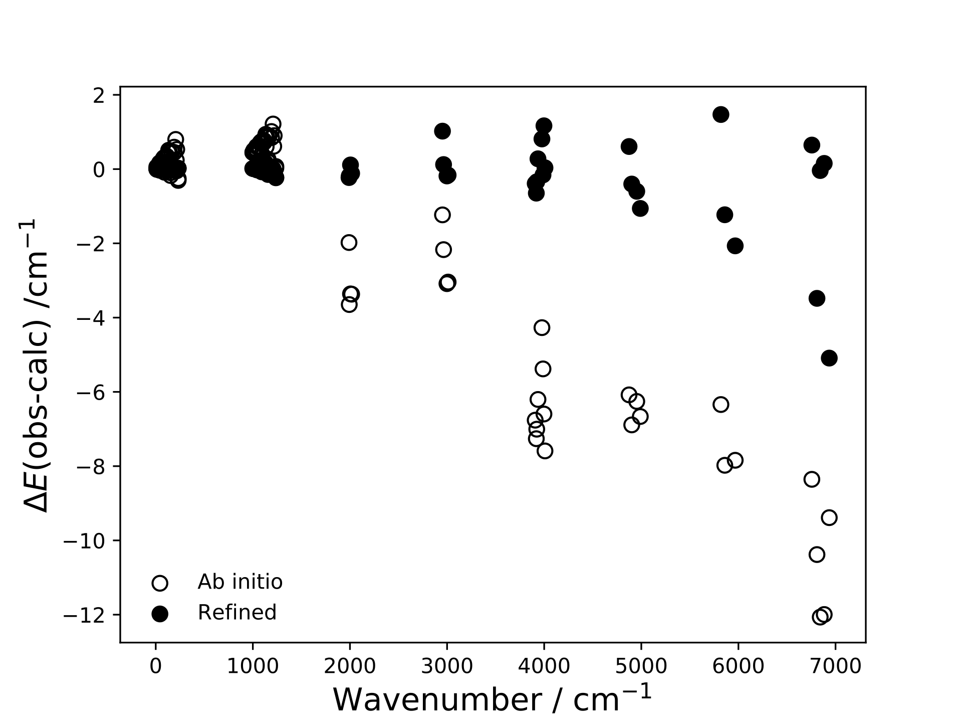
Figure 1: Residuals (observed-calculated) for the ab initio (empty circles) and the refined (full circles) term values from Table LABEL:t:obs-calc.

The equilibrium geometry was refined to the ground state rotational energy levels up to $J=5$, yielding the values $r_{\rm e}=1.51440$ Å and $\alpha_{\rm e}=92.005^{\circ}$. These are almost identical to the experimental values $r_{\rm exp}=1.5137\,\pm\,0.0003$ Å and $\alpha_{\rm exp}=92.04\,\pm\,0.05^{\circ}$, derived in a combined analysis of high-resolution spectroscopic data of SiH₂, SiHD and SiD₂ [2]. Both the ab initio and refined PESs of SiH₂ are provided as part of the supplementary material along with a Fortran routine to construct the surfaces.

3 The CATS line list

Table 2: Extract from the .states file of the CATS line list

$i$	$\tilde{E}_{i}$	$g_{i}$	$J$	$\Gamma_{\textrm{tot}}$	$v_{1}$	$v_{2}$	$v_{3}$	$\Gamma_{\textrm{vib}}$	$K_{a}$	$K_{c}$	$\tau_{\textrm{rot}}$	$\Gamma_{\textrm{rot}}$	$C_{i}$	$n_{1}$	$n_{2}$	$n_{3}$
1527	19978.952397	3	1	A2	2	8	5	B2	0	1	B1	0.98	2	5	8
1528	19982.538080	3	1	A2	0	20	1	B2	0	1	B1	0.98	0	1	20
1529	19986.504561	3	1	A2	10	2	1	B2	0	1	B1	-0.99	0	11	2
1530	19988.143253	3	1	A2	11	2	0	A1	1	1	A2	0.99	0	11	2
1531	10.721260	9	1	B1	0	0	0	A1	0	1	B1	1.00	0	0	0
1532	1009.393331	9	1	B1	0	1	0	A1	0	1	B1	-1.00	0	0	1
1533	1989.081019	9	1	B1	0	2	0	A1	0	1	B1	1.00	0	0	2
1534	2004.596674	9	1	B1	0	0	1	B2	1	1	A2	-1.00	0	1	0
1535	2016.232068	9	1	B1	1	0	0	A1	0	1	B1	1.00	1	0	0
1536	2962.467155	9	1	B1	0	3	0	A1	0	1	B1	-1.00	0	0	3

$i$: State counting number;
$\tilde{E}_{i}$: State energy in cm^-1;
$g_{i}$: State degeneracy;
$J$: Total angular momentum quantum number;
$\Gamma_{\textrm{tot}}$: Overall symmetry of state in ${\mathcal{C}}_{2{\rm v}}$(M);
$v_{1}$–$v_{3}$: Vibrational (normal mode) quantum numbers;
$\Gamma_{\textrm{vib}}$: Vibrational symmetry in ${\mathcal{C}}_{2{\rm v}}$(M);
$K_{a}$: Asymmetric top quantum number;
$K_{c}$: Asymmetric top quantum number;
$\tau_{\textrm{rot}}$: Rotational parity (0 or 1);
$\Gamma_{\textrm{rot}}$: Rotational symmetry in ${\mathcal{C}}_{2{\rm v}}$(M);
$C_{i}$: Largest coefficient used in the TROVE assignment;
$n_{1}$–$n_{3}$: Vibrational (TROVE) quantum numbers.

Table 3: Extract from the .trans file of the CATS line list

$f$	$i$	$A_{fi}$
149895	153613	1.0606e-06
24599	22431	1.0490e-01
284830	306093	6.3416e-10
74616	84147	6.5034e-08
186408	165765	1.1144e-07
84280	100878	4.1022e-07
224529	228578	2.8423e-04
54609	46478	1.4376e-02
142008	130207	3.6173e-10

$f$: Upper state ID counting number;

$i$: Lower state ID counting number;

$A_{fi}$: Einstein $A$ coefficient in s^-1.

The CATS line list contains 254 061 207 transitions connecting 369 973 ro-vibrational states and is provided in the ExoMol data format [17]. Extracts from the .states and .trans files are given in Tables 2 and 3, respectively. The .states file contains all the computed ro-vibrational energy levels (in cm^-1). Each level has a unique state counting number, symmetry and quantum number labelling and the contribution $C_{i}$ from the largest eigen-coefficient used to assign the ro-vibrational state in TROVE. The .trans files are split into ten 1000 cm^-1 wavenumber windows and contain all the computed transitions with upper and lower state ID labels and Einstein $A$ coefficients.

The normal mode quantum numbers $v_{1}$–$v_{3}$ were first reconstructed for $J=0$ and then propagated to all ro-vibrational states. These are related to the TROVE (local mode) vibrational quantum numbers $n_{1}$–$n_{3}$ as follows:

$$v_{1}+v_{3} = n_{1}+n_{2}\quad({\rm stretching}),$$ (23)

$$v_{3}\;({\rm odd})\quad \leftrightarrow \quad(n_{1},n_{2})B_{2},$$ (24)

$$v_{2} = n_{3}\quad({\rm bending}).$$ (25)

In correlating the normal mode $(v_{1},v_{3})$ and local mode $(n_{1},n_{2})$ pairs we also assumed that the energy increases with $v_{3}$. The asymmetric top quantum number $K_{a}$ coincides with the TROVE rotational quantum number $K$. The corresponding quantum number $K_{c}$ was obtained using the symmetry properties of the oblate rotor [45], see Table 4. Because of the way TROVE builds the symmetrized ro-vibrational basis set [40], the connection between the assignment and the primitive basis functions is not always straightforward and in cases of very small values of $|C_{i}|$, the assignment should be regarded as indicative.

Table 4: Symmetry properties of the $J_{K_{a},K_{c}}$ states of SiH₂ in the ${\mathcal{C}}_{2{\rm v}}$(M) symmetry group [45].

$K_{a}$	$K_{c}$	$\Gamma_{\rm rot}$		$K_{a}$	$K_{c}$	$\Gamma_{\rm rot}$
Even	Even	$A_{1}$		Odd	Even	$B_{2}$
Even	Odd	$B_{1}$		Odd	Odd	$A_{2}$

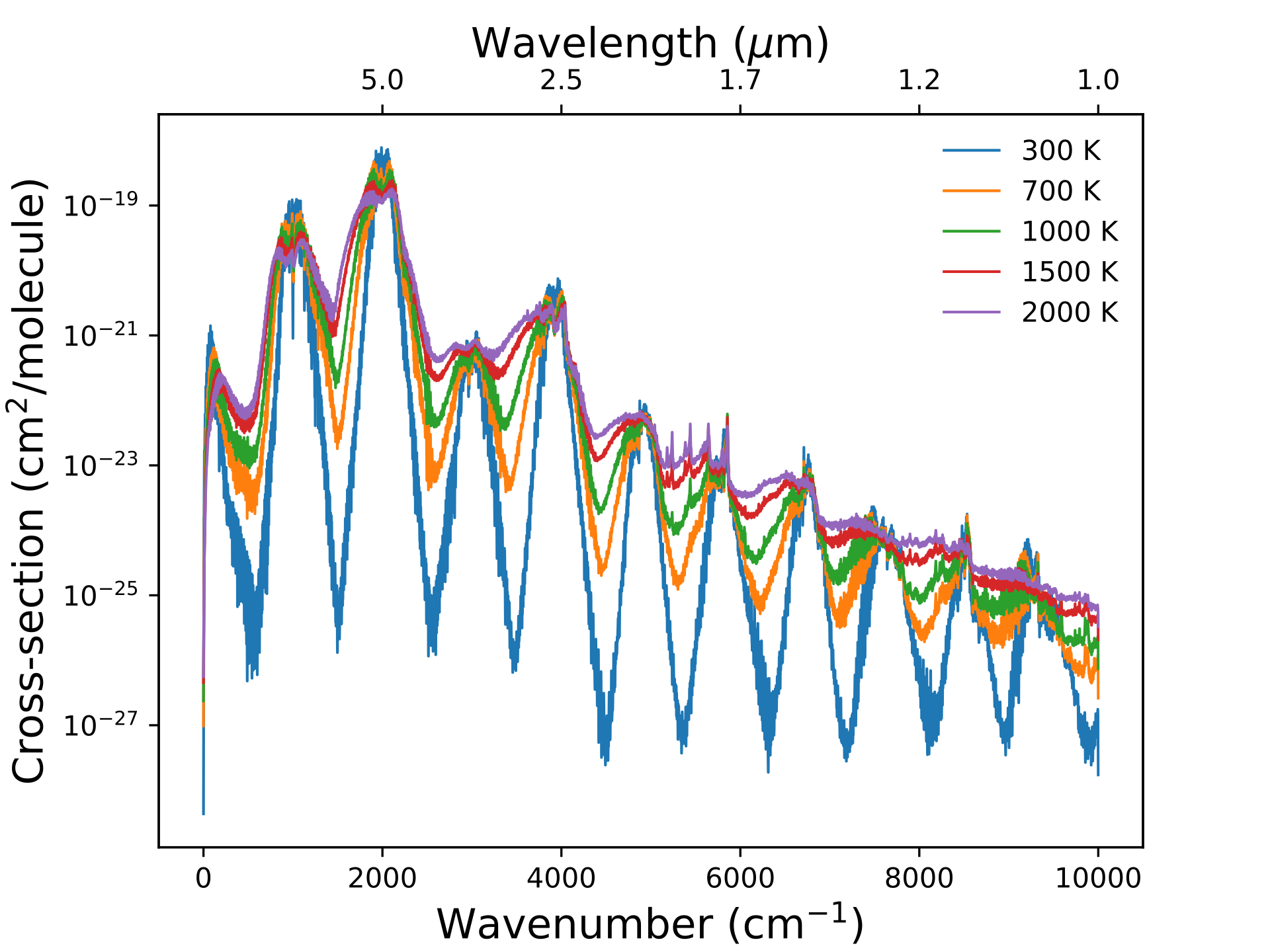
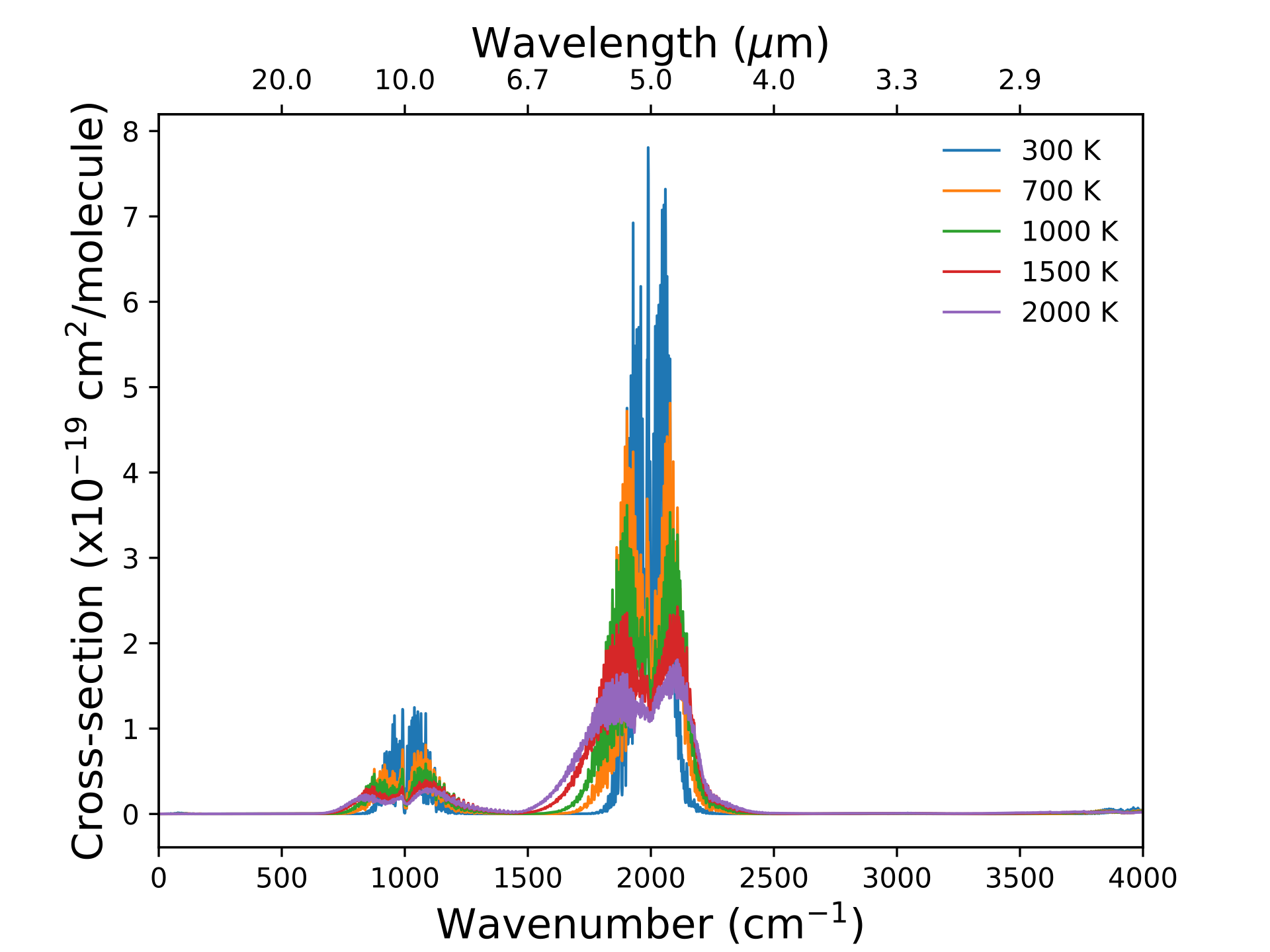
Figure 2: Absorption cross-sections of SiH₂ for various temperatures. Left: 0–10 000 cm^-1 range (logarithmic scale); Right: 0–4000 cm^-1 range (linear scale). Spectral simulations used a Gaussian line profile with HWHM of 1 cm^-1 at a resolution of 1 cm^-1.

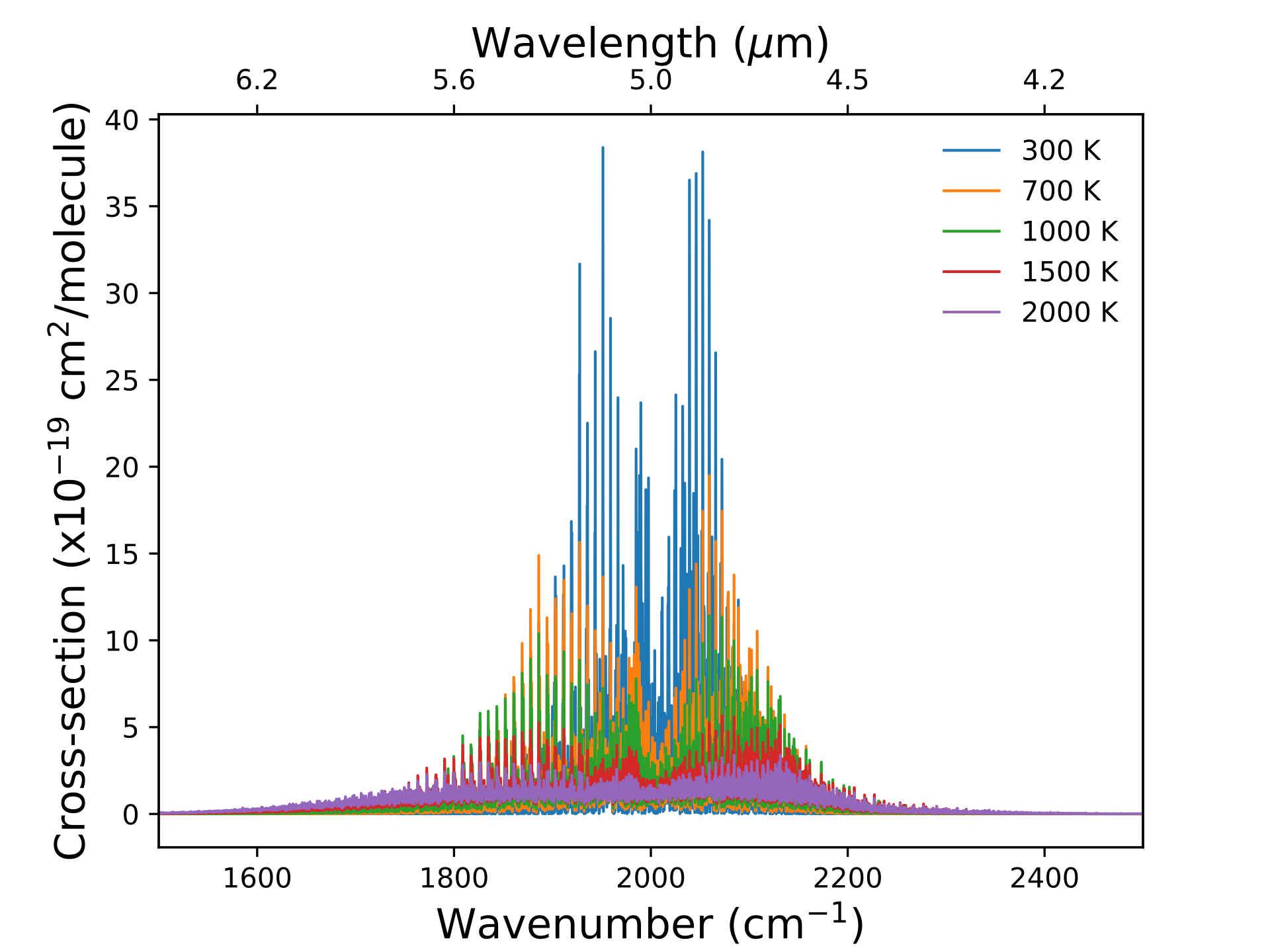
Figure 3: Absorption cross-sections of SiH₂ for various temperatures, focusing on the $\nu_{1}$ band. Spectral simulations used a Gaussian line profile with HWHM of 0.1 cm^-1 at a resolution of 0.1 cm^-1.

To illustrate the CATS line list, absorption cross-sections have been generated at 300, 700, 1000, 1500 and 2000 K and the results are shown in Figures 2 and 3. Spectral simulations used a Gaussian line profile and were performed with the ExoCross program [53]. In Fig. 2, the entire computed spectrum of SiH₂ is displayed at logarithmic scale and the linear scale is displayed up to 4000 cm^-1. The strongest bands of SiH₂ are 10 $\mu$m ($\nu_{2}$) and 5 $\mu$m ($2\nu_{2}$, $\nu_{1}$ and $\nu_{3}$), followed by the 2.5 $\mu$m ($2\nu_{1}$ and $2\nu_{3}$) bands, which agrees with the ro-vibrational spectrum from Ref. [12]. The pure rotational band is weak owing to the small equilibrium dipole moment of SiH₂. The corresponding values of the transition dipole moments are listed in Table 5. As the temperature increases, weaker band features become more prominent and the spectrum flattens. This can be seen in closer detail in Fig. 2 and Fig. 3.

Table 5: Vibrational transition dipole moments (TDM) for the strongest absorption bands of SiH₂ (Debye). The band centers (BC) are theoretical (TROVE) values (cm^-1).

Band	BC (cm-1)	TDM (Debye)
g.s.	0.00	0.1093
$\nu_{2}$	998.61	0.1752
$2\nu_{2}$	1978.35	0.1352
$\nu_{3}$	1993.00	0.2240
$\nu_{1}$	2005.54	0.1444
$3\nu_{2}$	2951.68	0.0029
$\nu_{2}+\nu_{3}$	2974.73	0.0036
$\nu_{1}+\nu_{2}$	2998.78	0.0076
$2\nu_{3}$	3907.79	0.0102
$\nu_{1}+\nu_{3}$	3913.39	0.0145
$2\nu_{1}$	3923.64	0.0092
$2\nu_{2}+\nu_{3}$	3952.47	0.0055

The first excited triplet state ($\tilde{a}^{3}B_{1}$) of SiH₂ is around 7000 cm^-1 [54] while the first excited singlet state ($\tilde{A}^{1}B_{1}$) lies at 15 500 cm^-1 [55]. The presence of these states would have had an effect on the accuracy of the computed ab initio PES and DMS, due to Renner-Teller and spin-orbit interactions between these electronic states, which were not taken into account here. Furthermore, the PES was only refined to term values below 7000 cm^-1. Use of the CATS line list above 7000 cm^-1, or for transitions originating from states above 7000 cm^-1, should therefore be treated with a degree of caution. That said, the associated transition intensities will be very weak and this should not overly affect the quality of the line list.

3.1 Partition function of silylene

The temperature-dependent partition function,

$$Q(T)=\sum_{i}g_{i}\exp\left(-\frac{E_{i}}{kT}\right),$$ (26)

where $g_{i}=g_{i}^{(\rm ns)}(2J_{i}+1)$ is the degeneracy of a state $i$ with energy $E_{i}$ and rotational quantum number $J_{i}$, has been evaluated at 1 K intervals in the range 0–2000 K. The convergence of $Q(T)$ is illustrated in Fig. 4 for $T$ = 300, 1000, 1500 and 2000 K. The flattening of all four lines indicates that convergence has been achieved after approximately $J$ = 10, 30, 40 and 50, respectively.

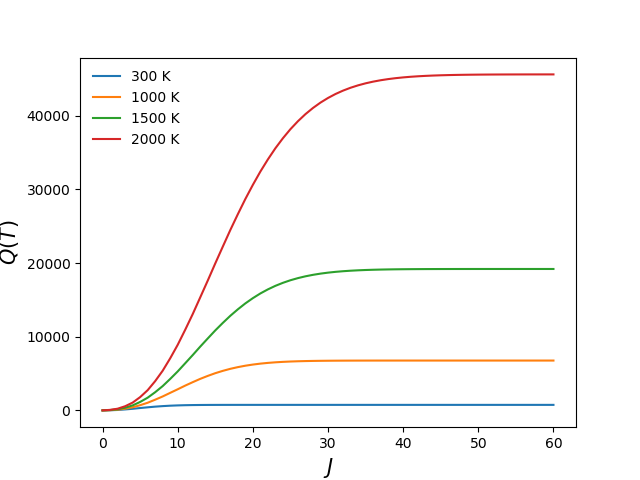
Figure 4: Convergence of the temperature-dependent partition function $Q(T)$ of SiH₂ against the rotational angular momentum quantum number $J$ at 300, 1000, 1500 and 2000 K.

4 Rotational energy level clustering

The equilibrium interbond angle of SiH₂ is close to 90^∘ with the masses of the hydrogen atoms significantly smaller than that of Si. These properties are known to lead to so-called rotational cluster states [56], where a group of rotational energy levels become quasi-degenerate at high rotational excitation. Dorney and Watson [57] were the first to explain cluster formation in terms of classical rotation about symmetrically equivalent axes associated with “stable” axes of rotation, about which the molecule prefers to rotate. Subsequently, Harter and co-workers (see, for example, Refs. [58, 59]) developed classical models for the description of cluster formation in XY_N molecules and introduced the concept of a rotational energy surface (RES), which defines the pattern of the rotational energy levels. The clustering of two or four quasi-degenerate energy levels corresponds classically to the appearance of two or four stable rotation axes, where clockwise and anticlockwise rotations are regarded independently. The two-fold degeneracy is the well known $K$-type doubling [60], while four-fold cluster states in XH₂-type molecules were predicted [61, 62, 63, 64, 65, 66, 67, 23] and first observed in the H₂Se molecule [68, 69, 70].

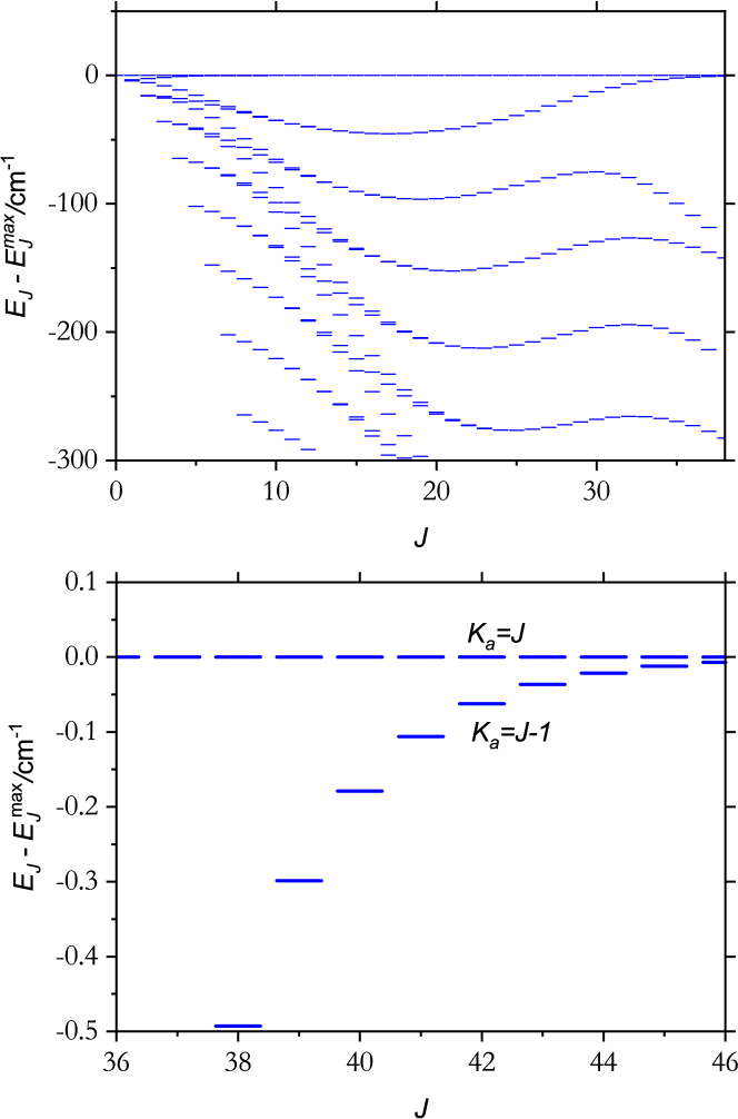
Figure 5: Rotational energy level clustering in the ground vibrational state of SiH₂. In the top panel, the energy difference $\tilde{E}_{J,i}-\tilde{E}_{J,i}^{\rm max}$, see Eq. (27), has been plotted for each rotational state, with energy $\tilde{E}_{J,i}$ relative to the maximum energy $\tilde{E}_{J,i}^{\rm max}$ in its $J$ multiplet. After a certain critical $J$ value the energy difference begins to decrease leading to the formation of four-fold rotational cluster states. A close up of the first cluster state being formed is shown in the bottom panel.

In SiH₂, we have found that the rotational energies display typical four-fold clustering behaviour, illustrated in Fig. 5, where we have plotted the reduced rotational energy difference,

$$\tilde{E}_{J,i}^{\rm red}=\tilde{E}_{J,i}-\tilde{E}_{J,i}^{\rm max}.$$ (27)

Here, $\tilde{E}_{J,i}^{\rm max}$ is the maximal energy level for a given $J$-manifold, which for SiH₂ corresponds to $K_{a}=J$. As $J$ increases the separation between the two pairs of levels with $K_{a}=J$ ($K_{c}=0$ and $K_{c}=1$) and $K_{a}=J-1$ ($K_{c}=1$ and $K_{c}=2$) increases, which is common in asymmetric-top molecules. However, after a critical $J$ value of $J_{\rm cr}\approx 17$, this separation starts decreasing until four-fold cluster states form. For example, at $J=40$ in the top cluster (shown in the bottom panel of Fig. 5), the separation between the two pairs is only 0.2 cm^-1 but at $J=50$ this gap is reduced to 0.006 cm^-1. The pattern of the rotational energy levels in Fig. 5 is typical of most XH₂-type molecules [71, 69, 64, 66, 67].

As mentioned above, the four-fold clusters at high $J$ can be associated with the formation of stable rotation axes around the molecular bonds Si–H₁ and Si–H₂ with four equivalent rotational motions: clockwise/anticlockwise around the Si–H₁ and Si–H₂ bonds. These rotation axes are approximately at 45^∘ relative to the principal axes of the molecule $x$ axis (along the bisector) and $z$ axis (in plane). The other stable rotational direction is around the axis associated with the $x$ axis. The rotational motion is commonly illustrated using the rotational energy surface $E_{\theta,\phi}$ [58, 59], constructed as the minimum ro-vibrational energy for each orientation of the angular momentum vector $\vec{J}$ considered in the molecule-fixed axis system, where the orientation is described by a polar angle $\theta$ and an azimuthal angle $\phi$. Here $\theta$ $\in$ $[0,\pi]$ is the angle between $\vec{J}$ and the molecule-fixed $z$ axis and $\phi$ $\in$ $[0,2\pi]$ is the angle between the $x$ axis and the projection of $\vec{J}$ in the $xy$ plane, measured in the usual positive sense. In this picture, the RES is a manifestation of the pure rotational motion of a molecule with the vibrational motion completely frozen to the corresponding optimized geometry. If the rotational motion is classically represented by trajectories on the RES, the stationary points (zero-dimensional trajectories) represent rotation about the stabilization axes.

For SiH₂, we have constructed the RES from a classical ro-vibrational Hamiltonian $H_{\rm rv}$ with the $xyz$ components of the quantum-mechanical angular momentum operator ${\mathbf{J}}$ substituted by their classical analogues,

$$J_{x} = \sqrt{J(J+1)}\,\sin\theta\,\cos\phi$$ (28)

$$J_{y} = \sqrt{J(J+1)}\,\sin\theta\,\sin\phi$$ (29)

$$J_{z} = \sqrt{J(J+1)}\,\cos\theta\,\hbox{,}$$ (30)

with the generalized momenta $p_{n}$ $=$ $\partial T/\partial{\dot{q}}_{n}$ set to zero [68]. Here, $T$ is the classical kinetic energy and the momentum $p_{n}$ for $n=1,2,3$ is conjugate to the generalized coordinate $q_{n}$ $\in$ $\{r_{1},r_{2},\alpha\}$. The classical Hamiltonian $H_{\rm rv}$ was defined as the same Hamiltonian used in variational TROVE calculations. The RES $E_{J}(\theta,\phi)$ is then given by [72, 73]

$$E_{J}(\theta,\phi)=H_{\rm rv}(J,r_{i}=r_{i}^{\rm opt},\alpha=\alpha^{\rm opt},\theta,\phi)\hbox{,}$$ (31)

where the classical Hamiltonian function $H_{\rm rv}$ is calculated at the optimized geometries $r_{i}^{\rm opt},\alpha^{\rm opt}$ for each orientation of the angular momentum defined by the polar and azimuthal angles $(\theta,\phi)$. The RES was computed on a regular grid of angular points $\theta_{m},\phi_{m}$. The bond lengths $r_{1}$ and $r_{2}$ and the bond angle $\alpha$ were optimized at each grid point by minimizing the classical energy $E=H_{\rm rv}(r_{i},\alpha_{i},\theta_{m},\phi_{m})$.

The RES of SiH₂ at $J=40$ is shown in Figs. 6 and 7, computed on a $40\times 80$ grid ($\theta,\phi$) of points. The two minima ($\theta=0$ and $180^{\circ}$) and four maxima ($\theta=36^{\circ}$ and $\theta=144^{\circ}$, $\phi=0^{\circ}$ and 180^∘ ) form the stationary points of the semi-classical description of the rotation of SiH₂ and can be used to interpret the rotational clustering in the quantum-mechanical description: $n$-fold degenerate energy clusters [58, 74] correspond to a RES with $n$ symmetrically equivalent stationary points. Coriolis-type effects break the ${\mathcal{C}}_{2{\rm v}}$ symmetry of the molecule in the cluster states. For example, the optimized geometry corresponding to the stationary point at $\theta=36^{\circ},\phi=0$ ($J=40$) was found to be $r_{1}=1.519$ Å, $r_{2}=1.648$ Å and $\alpha=87^{\circ}$. See also Ref. [71] on the bifurcation of stationary points and how it affects the formation of rotational energy clusters.

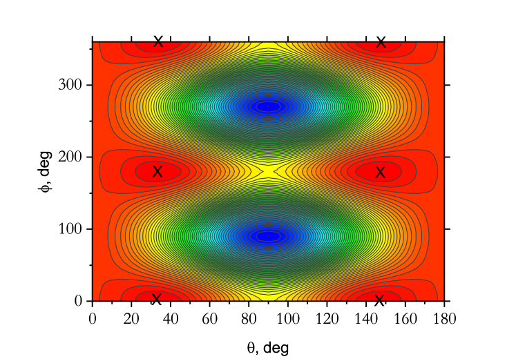
Figure 6: The rotational energy surface of SiH₂ calculated at $J=40$. The four equivalent maxima corresponding to the four-fold rotational clusters are indicted with crosses. The colour (red to blue) represents the energy scale (high to low).

Figure 7: A one-dimensional slice at $\phi=0^{\circ}$ of the rotational energy surface (RES) of SiH₂ calculated at $J=40$ (cm^-1). The two equivalent maxima are found at $\theta=36$ and $144^{\circ}$.

5 Conclusion

The first, comprehensive high-temperature rotation-vibration line list, named CATS, has been calculated for the electronic ground state of SiH₂ using a refined PES and a high level ab initio DMS. The line list covers the wavenumber range 0–10 000 cm^-1 and is applicable for temperatures up to $T=2000$ K and represent an improvement for the ro-vibrational spectra of SiH₂ predicted in Refs. [12, 13]. The CATS line list is available from the ExoMol database [16, 17] at www.exomol.com which already contains line lists for SiH₄ [18] and SiH [19]. There are also recent experimental studies on SiH₃ [6]. These line lists will facilitate spectroscopic studies on silane plasmas. It is also hoped that our work will stimulate more investigations into SiH₂ to enable our theoretical spectroscopic model to be benchmarked and improved upon.

We have demonstrated that SiH₂ forms rotational energy level clusters at high rotational excitation and established the critical $J$ value of $J_{\rm cr}\approx 17$ when the effect first becomes noticable. Cluster states are intimately linked to the phenomenon of rotationally-induced chirality in the motion of small polyatomic molecules [75] and the use of techniques from strong-field laser physics [76] can be utilised to produce dynamically chiral molecules through extreme rotational excitation [77].

The CATS line list should find use in plasma physics and the monitoring of SiH₂ in different processes and reactions. Since silylene is a radical and highly reactive, whether it can accumulate in large enough quantities to be detected astronomically is debatable. As discussed above, given the complicated electronic structure of SiH₂ and the relatively low-lying $\tilde{a}^{3}B_{1}$ and $\tilde{A}^{1}B_{1}$ excited states, some caution should be exercised when using the line list above 7000 cm^-1, or for transitions originating from states above 7000 cm^-1. That said, the associated transition intensities will be very weak and we do not expect the quality of the CATS line list to be significantly affected.

References

- [1] I. Dubois, G. Herzberg, R. D. Verma, Spectrum of SiH2, J. Chem. Phys. 47 (10) (1967) 4262. doi:10.1063/1.1701609.
- [2] D. L. Kokkin, T. Ma, T. Steimle, T. J. Sears, Detection and characterization of singly deuterated silylene, SiHD, via optical spectroscopy, J. Chem. Phys. 144 (24) (2016) 244304. doi:10.1063/1.4954702.
- [3] J. Jasinski, B. S. Meyerson, B. A. Scott, Mechanistic studies of chemical vapor-deposition, Ann. Rev. Phys. Chem. 38 (1987) 109–140. doi:10.1146/annurev.physchem.38.1.109.
- [4] J. R. Doyle, D. A. Doughty, A. Gallagher, Silane Dissociation Products in Deposition Discharges, J. Appl. Phys. 68 (9) (1990) 4375–4384. doi:10.1063/1.346186.
- [5] J. Jasinski, J. O. Chu, Absolute rate constants for the reaction of silylene with hydrogen, silane, and disilane, J. Chem. Phys. 88 (1988) 1678–1687. doi:10.1063/1.454146.
- [6] A. S. Nave, A. V. Pipa, P. B. Davies, J. Roepcke, J.-P. H. van Heiden, Determining a Line Strength in the Band of the Silyl Radical Using Quantum Cascade Laser Absorption Spectroscopy, J. Phys. A: Math. Gen. 123 (46) (2019) 10030–10039. doi:10.1021/acs.jpca.9b06351.
-
[7]
B. E. Turner, Detection of
SiN in IRC + 10216, Astrophys. J. 388 (1992) L35.
doi:10.1086/186324.
URL http://adsabs.harvard.edu/doi/10.1086/186324 - [8] L. W. Avery, M. B. Bell, C. T. Cunningham, P. A. Feldman, R. H. Hayward, J. M. Macleod, H. E. Matthews, J. D. Wade, Submillimeter molecular line observations of IRC+10216: Searches for MgH, SiH2, and HCO+, and detection of hot HCN, Astrophys. J. 426 (2,1) (1994) 737–741. doi:10.1086/174110.
-
[9]
D. D. S. MacKay, S. B. Charnley,
The silicon chemistry
of IRC+10216, Mon. Not. R. Astron. Soc. 302 (4) (1999) 793–800.
doi:10.1046/j.1365-8711.1999.02175.x.
URL https://doi.org/10.1046/j.1365-8711.1999.02175.x - [10] Y. Apeloig, R. Pauncz, M. Karni, R. West, W. Steiner, D. Chapman, Why is methylene a ground state triplet while silylene is a ground state singlet?, Organometallics 22 (16) (2003) 3250–3256. doi:10.1021/om0302591.
- [11] A. Kalemos, T. H. Dunning, A. Mavridis, SiH2, a critical study, Mol. Phys. 102 (23-24) (2004) 2597–2606. doi:10.1080/00268970412331293802.
- [12] W. Gabriel, P. Rosmus, K. Yamashita, K. Morokuma, P. Palmieri, Theoretical rotational vibrational-spectrum of SiH2 ( and ), Chem. Phys. 174 (1) (1993) 45–56. doi:10.1016/0301-0104(93)80050-J.
- [13] S. N. Yurchenko, P. R. Bunker, W. P. Kraemer, P. Jensen, The spectrum of singlet SiH2, Can. J. Chem. 82 (6) (2004) 694–708. doi:10.1139/V04-030.
- [14] R. Guerout, P. R. Bunker, P. Jensen, W. P. Kraemer, A calculation of the rovibronic energies and spectrum of the electronic state of SiH2, J. Chem. Phys. 123 (24) (2005) 244312. doi:10.1063/1.2139676.
- [15] J. Tennyson, Perspective: Accurate ro-vibrational calculations on small molecules, J. Chem. Phys. 145 (2016) 120901. doi:10.1063/1.4962907.
- [16] S. N. Yurchenko, J. Tennyson, ExoMol: molecular line lists for exoplanet and other atmospheres, in: C. Stehlé, C. Jobin, L. d’Hendercourt (Eds.), European Conference on Laboratory Astrophysics – ECLA, Vol. 58 of Euro. Astron. Soc. Publications Series, 2012, pp. 243–248.
- [17] J. Tennyson, S. N. Yurchenko, A. F. Al-Refaie, E. J. Barton, K. L. Chubb, P. A. Coles, S. Diamantopoulou, M. N. Gorman, C. Hill, A. Z. Lam, L. Lodi, L. K. McKemmish, Y. Na, A. Owens, O. L. Polyansky, T. Rivlin, C. Sousa-Silva, D. S. Underwood, A. Yachmenev, E. Zak, The ExoMol database: molecular line lists for exoplanet and other hot atmospheres, J. Mol. Spectrosc. 327 (2016) 73–94. doi:10.1016/j.jms.2016.05.002.
- [18] A. Owens, S. N. Yurchenko, A. Yachmenev, W. Thiel, J. Tennyson, ExoMol molecular line lists XXII. The rotation-vibration spectrum of silane up to 1200 K, Mon. Not. R. Astron. Soc. 471 (2017) 5025–5032. doi:10.1093/mnras/stx1952.
- [19] M. Gorman, S. N. Yurchenko, J. Tennyson, ExoMol Molecular linelists – XXXVI. – and – transitions of SH, Mon. Not. R. Astron. Soc. 490 (2019) 1652–1665. doi:10.1093/mnras/stz2517/5565070.
- [20] E. J. Barton, S. N. Yurchenko, J. Tennyson, ExoMol Molecular linelists – II. The ro-vibrational spectrum of SiO, Mon. Not. R. Astron. Soc. 434 (2013) 1469–1475.
- [21] A. Upadhyay, E. K. Conway, J. Tennyson, S. N. Yurchenko, ExoMol Molecular linelists – XXV: A hot line list for silicon sulphide, SiS, Mon. Not. R. Astron. Soc. 477 (2018) 1520–1527. doi:10.1093/mnras/sty998.
- [22] J. Tennyson, S. N. Yurchenko, The ExoMol project: Software for computing molecular line lists, Intern. J. Quantum Chem. 117 (2017) 92–103. doi:10.1002/qua.25190.
- [23] P. Jensen, An introduction to the theory of local mode vibrations, Mol. Phys. 98 (17) (2000) 1253–1285. doi:10.1080/002689700413532.
- [24] C. Hätig, D. P. Tew, A. Köhn, Communications: Accurate and efficient approximations to explicitly correlated coupled-cluster singles and doubles, CCSD-F12, J. Chem. Phys. 132 (23) (2010) 231102. doi:10.1063/1.3442368.
- [25] K. A. Peterson, T. B. Adler, H.-J. Werner, Systematically convergent basis sets for explicitly correlated wavefunctions: The atoms H, He, B–Ne, and Al-Ar, J. Chem. Phys. 128 (8) (2008) 084102. doi:10.1063/1.2831537.
- [26] S. Ten-No, Initiation of explicitly correlated Slater-type geminal theory, Chem. Phys. Lett. 398 (1-3) (2004) 56–61. doi:10.1016/j.cplett.2004.09.041.
- [27] J. G. Hill, K. A. Peterson, G. Knizia, H.-J. Werner, Extrapolating MP2 and CCSD explicitly correlated correlation energies to the complete basis set limit with first and second row correlation consistent basis sets, J. Chem. Phys. 131 (19) (2009) 194105. doi:10.1063/1.3265857.
- [28] K. E. Yousaf, K. A. Peterson, Optimized auxiliary basis sets for explicitly correlated methods, J. Chem. Phys. 129 (18) (2008) 184108. doi:10.1063/1.3009271.
- [29] F. Weigend, A fully direct RI-HF algorithm: Implementation, optimised auxiliary basis sets, demonstration of accuracy and efficiency, Phys. Chem. Chem. Phys. 4 (2002) 4285–4291. doi:10.1039/B204199P.
- [30] C. Hättig, Optimization of auxiliary basis sets for RI-MP2 and RI-CC2 calculations: Core-valence and quintuple-zeta basis sets for H to Ar and QZVPP basis sets for Li to Kr, Phys. Chem. Chem. Phys. 7 (2005) 59–66. doi:10.1039/b415208e.
- [31] H.-J. Werner, P. J. Knowles, G. Knizia, F. R. Manby, M. Schütz, Molpro: a general-purpose quantum chemistry program package, WIREs Comput. Mol. Sci. 2 (2012) 242–253. doi:10.1002/wcms.82.
- [32] V. G. Tyuterev, S. A. Tashkun, D. W. Schwenke, An accurate isotopically invariant potential function of the hydrogen sulphide molecule, Chem. Phys. Lett. 348 (2001) 223–234. doi:10.1016/S0009-2614(01)01093-4.
- [33] H. Partridge, D. W. Schwenke, The determination of an accurate isotope dependent potential energy surface for water from extensive ab initio calculations and experimental data, J. Chem. Phys. 106 (1997) 4618–4639. doi:10.1063/1.473987.
- [34] J. K. G. Watson, Robust weighting in least-square fits, J. Mol. Spectrosc. 219 (2003) 326–328. doi:10.1016/S0022-2852(03)00100-0.
- [35] P. Jensen, Calculation of rotation-vibration linestrengths for triatomic molecules using a variational approach: Application to the fundamental bands of CH2, J. Mol. Spectrosc. 132 (1988) 429 – 457. doi:http://dx.doi.org/10.1016/0022-2852(88)90338-4.
- [36] U. G. Jørgensen, P. Jensen, The dipole-moment surface and the vibrational transition moments of H2O, J. Mol. Spectrosc. 161 (1993) 219–242. doi:10.1006/jmsp.1993.1228.
- [37] A. A. A. Azzam, L. Lodi, S. N. Yurchenko, J. Tennyson, The dipole moment surface for hydrogen sulfide H2S, J. Quant. Spectrosc. Radiat. Transf. 161 (2015) 41–49. doi:10.1016/j.jqsrt.2015.03.029.
- [38] S. N. Yurchenko, W. Thiel, P. Jensen, Theoretical ROVibrational Energies (TROVE): A robust numerical approach to the calculation of rovibrational energies for polyatomic molecules, J. Mol. Spectrosc. 245 (2007) 126–140. doi:10.1016/j.jms.2007.07.009.
- [39] A. Yachmenev, S. N. Yurchenko, Automatic differentiation method for numerical construction of the rotational-vibrational Hamiltonian as a power series in the curvilinear internal coordinates using the Eckart frame, J. Chem. Phys. 143 (2015) 014105. doi:10.1063/1.4923039.
-
[40]
S. N. Yurchenko, A. Yachmenev, R. I. Ovsyannikov,
Symmetry adapted
ro-vibrational basis functions for variational nuclear motion: TROVE
approach, J. Chem. Theory Comput. 13 (9) (2017) 4368–4381.
arXiv:http://dx.doi.org/10.1021/acs.jctc.7b00506, doi:10.1021/acs.jctc.7b00506.
URL http://dx.doi.org/10.1021/acs.jctc.7b00506 - [41] B. V. Noumerov, A method of extrapolation of perturbations, Mon. Not. R. Astron. Soc. 84 (1924) 592–602. doi:10.1093/mnras/84.8.592.
- [42] J. W. Cooley, An improved eigenvalue corrector formula for solving the Schrödinger equation for central fields, Math. Comp. 15 (1961) 363–374. doi:10.1090/S0025-5718-1961-0129566-X.
- [43] K. L. Chubb, P. Jensen, S. N. Yurchenko, Symmetry adaptation of the rotation-vibration theory for linear molecules, Symmetry 10 (5) (2018) 137. doi:10.3390/sym10050137.
- [44] K. L. Chubb, A. Yachmenev, J. Tennyson, S. N. Yurchenko, Treating linear molecule HCCH in calculations of rotation-vibration spectra, J. Chem. Phys. 149 (2018) 014101. doi:10.1063/1.5031844.
- [45] P. R. Bunker, P. Jensen, Molecular Symmetry and Spectroscopy, 2nd Edition, NRC Research Press, Ottawa, 1998.
- [46] S. N. Yurchenko, R. J. Barber, J. Tennyson, W. Thiel, P. Jensen, Towards efficient refinement of molecular potential energy surfaces: Ammonia as a case study, J. Mol. Spectrosc. 268 (2011) 123–129. doi:10.1016/j.jms.2011.04.005.
- [47] C. Yamada, H. Kanamori, E. Hirota, N. Nishiwaki, N. Itabashi, K. Kato, T. Goto, Detection of the silylene band by infrared diode laser kinetic spectroscopy, J. Chem. Phys. 91 (8) (1989) 4582–4586. doi:10.1063/1.456746.
- [48] H. Ishikawa, O. Kajimoto, Fermi resonance and vibrational analysis of SiH2 () based on the LIF excitation-spectra of the transitions, J. Mol. Spectrosc. 150 (2) (1991) 610–619. doi:10.1016/0022-2852(91)90252-6.
- [49] E. Hirota, H. Ishikawa, The vibrational spectrum and molecular constants of silicon dihydride SiH2 in the ground electronic state, J. Chem. Phys. 110 (9) (1999) 4254–4257. doi:10.1063/1.478308.
- [50] H. Ishikawa, Y. Muramoto, N. Mikami, Stimulated emission pumping spectroscopy of SiH2: First observation of the spin-orbit interaction between the A(1) and the states, J. Mol. Spectrosc. 216 (1) (2002) 90–97. doi:10.1006/jmsp.2002.8666.
- [51] C. M. Western, PGOPHER: A program for simulating rotational, vibrational and electronic spectra , J. Quant. Spectrosc. Radiat. Transf. 186 (2017) 221–242. doi:10.1016/j.jqsrt.2016.04.010.
- [52] S. N. Yurchenko, M. Carvajal, P. Jensen, F. Herregodts, T. R. Huet, Potential parameters of PH3 obtained by simultaneous fitting of ab initio data and experimental vibrational band origins, Chem. Phys. 290 (2003) 59–67. doi:10.1016/S0301-0104(03)00098-3.
- [53] S. N. Yurchenko, A. F. Al-Refaie, J. Tennyson, ExoCross: a general program for generating spectra from molecular line lists, Astron. Astrophys. 614 (2018) A131. doi:10.1051/0004-6361/201732531.
-
[54]
J. Berkowitz, J. P. Greene, H. Cho, B. Ruščić,
Photoionization mass spectrometric
studies of SiH (), J. Chem. Phys. 86 (3) (1987) 1235–1248.
doi:10.1063/1.452213.
URL https://doi.org/10.1063/1.452213 - [55] R. Escribano, A. Campargue, Absorption spectroscopy of SiH2 near 640 nm, J. Chem. Phys. 108 (15) (1998) 6249–6257. doi:10.1063/1.476062.
- [56] P. Jensen, G. Osmann, I. N. Kozin, The Formation of Four-fold Rovibrational Energy Clusters in H2S, H2Se, and H2Te, in: D. Papousek (Ed.), Advanced Series in Physical Chemistry: Vibration-Rotational Spectroscopy and Molecular Dynamics, Vol. 9, World Scientific Publishing Company, Singapore, 1997, pp. 298–351.
- [57] A. J. Dorney, J. K. G. Watson, Forbidden Rotational Spectra of Polyatomic-Molecules Stark Effects and Transitions of Molecules, J. Mol. Spectrosc. 42 (1972) 135–148. doi:10.1016/0022-2852(72)90150-6.
- [58] W. G. Harter, C. W. Patterson, Rotational Energy Surfaces and High- Eigenvalue Structure of Polyatomic-Molecules, J. Chem. Phys. 80 (1984) 4241–4261. doi:10.1063/1.447255.
- [59] W. G. Harter, Computer Graphical and Semiclassical Approaches to Molecular Rotations and Vibrations, Comp. Phys. Rep. 8 (1988) 319–394. doi:10.1016/0167-7977(88)90011-1.
- [60] D. Papoušek, M. R. Aliev, Molecular Vibrational-Rotational Spectra, Elsevier, Amsterdam, 1982.
- [61] B. I. Zhilinsky, I. M. Pavlichenkov, Critical Effect in Rotational Spectra of Water Molecule, Opt. Spektrosk. 64 (1988) 688–690.
- [62] K. K. Lehmann, The interaction of rotation and local mode tunneling in the overtone spectra of symmetrical hydrides, J. Chem. Phys. 95 (4) (1991) 2361–2370. doi:10.1063/1.460942.
- [63] I. N. Kozin, S. Klee, P. Jensen, O. L. Polyansky, I. M. Pavlichenkov, The Far-Infrared Fourier-Transform Spectrum of H2Se, J. Mol. Spectrosc. 158 (1993) 409–422. doi:10.1006/jmsp.1993.1085.
- [64] I. N. Kozin, P. Jensen, Fourfold Clusters of Rovibrational Energy-Levels for H2S Studied With a Potential-Energy Surface Derived From Experiment, J. Mol. Spectrosc. 163 (1994) 483–509. doi:10.1006/jmsp.1994.1041.
- [65] I. N. Kozin, I. M. Pavlichenkov, Bifurcation in rotational spectra of nonlinear AB2 molecules, J. Chem. Phys. 104 (1996) 4105–4113. doi:10.1063/1.471223.
- [66] I. N. Kozin, P. Jensen, O. Polanz, S. Klee, L. Poteau, J. Demaison, The Rotational Spectrum of H2Te, J. Mol. Spectrosc. 180 (2) (1996) 402–413.
-
[67]
P. Gómez, L. Pacios, P. Jensen,
Fourfold
Clusters of Rovibrational Energies in H2Po Studied with an Ab
Initio Potential Energy Function, J. Mol. Spectrosc. 186 (1) (1997) 99 –
104.
doi:https://doi.org/10.1006/jmsp.1997.7434.
URL http://www.sciencedirect.com/science/article/pii/S0022285297974348 - [68] I. N. Kozin, P. Jensen, Fourfold Clusters of Rovibrational Energy-Levels in the Fundamental Vibrational-States if H2Se, J. Mol. Spectrosc. 161 (1993) 186–207. doi:10.1006/jmsp.1993.1226.
- [69] P. Jensen, I. N. Kozin, The Potential-Energy Surface for the Electronic Ground-State of H2Se Derived from Experiment, J. Mol. Spectrosc. 160 (1993) 39–57. doi:10.1006/jmsp.1993.1155.
- [70] J. M. Flaud, C. Camy-Peyret, H. Burger, P. Jensen, I. N. Kozin, Experimental-Evidence for the Formation of Fourfold Rovibrational Energy Clusters in the Vibrational-States of HSe, J. Mol. Spectrosc. 172 (1995) 126–134. doi:10.1006/jmsp.1995.1161.
- [71] I. M. Pavlichenkov, B. I. Zhilinskií, Critical phenomena in rotational spectra, Ann. Phys. 184 (1988) 1–32. doi:10.1016/0003-4916(88)90268-0.
- [72] S. N. Yurchenko, W. Thiel, S. Patchkovskii, P. Jensen, Theoretical evidence for the formation of rotational energy level clusters in the vibrational ground state of PH3, Phys. Chem. Chem. Phys. 7 (2005) 573–582. doi:10.1039/b418073a.
- [73] S. N. Yurchenko, W. Thiel, P. Jensen, Rotational energy cluster formation in XY3 molecules: Excited vibrational states of BiH3 and SbH3, J. Mol. Spectrosc. 240 (2006) 174–187. doi:10.1016/j.jms.2006.10.002.
-
[74]
J. Makarewicz, Semiclassical
and quantum mechanical pictures of the ro-vibrational motion of triatomic
molecules, Mol. Phys. 69 (5) (1990) 903–921.
arXiv:https://doi.org/10.1080/00268979000100681, doi:10.1080/00268979000100681.
URL https://doi.org/10.1080/00268979000100681 - [75] P. R. Bunker, P. Jensen, Chirality in rotational energy level clusters, J. Mol. Spectrosc. 228 (2004) 640–644. doi:10.1016/j.jms.2004.02.027.
-
[76]
A. Owens, A. Yachmenev, J. Küpper,
Coherent control of the
rotation axis of molecular superrotors, J. Phys. Chem. Lett. 9 (15) (2018)
4206–4209.
doi:10.1021/acs.jpclett.8b01689.
URL https://doi.org/10.1021/acs.jpclett.8b01689 - [77] A. Owens, A. Yachmenev, S. N. Yurchenko, J. Küpper, Climbing the rotational ladder to chirality, Phys. Rev. Lett. 121 (2018) 193201. doi:10.1103/PhysRevLett.121.193201.