Drive-noise tolerant optical switching inspired by composite pulses

Abstract

Electro-optic modulators within Mach–Zehnder interferometers are a common construction for optical switches in integrated photonics. A challenge faced when operating at high switching speeds is that noise from the electronic drive signals will effect switching performance. Inspired by the Mach–Zehnder lattice switching devices of Van Campenhout et al. [Opt. Express, 17, 23793 (2009)] and techniques from the field of Nuclear Magnetic Resonance known as composite pulses, we present switches which offer protection against drive-noise in both the on and off state of the switch for both the phase and intensity information encoded in the switched optical mode.

I Introduction

Optical switching is a key tool in many areas of integrated photonics. For example, it is thought that optical switching may be useful in removing inter-chip Shacham et al. (2008); Sun et al. (2015); Miller (2009) and intra-chip Cheng et al. (2018) communication bottlenecks in future classical computing architectures. Optical switching also finds applications in many proposed platforms for quantum computing. Several architectures use optical switching networks for connecting matter based quantum bits (qubits) via single photon entangling gates, allowing for distributed architectures Monroe et al. (2014); Nickerson et al. (2014); Choi et al. (2019). Linear optical quantum computing (LOQC) uses single photons for both transportation and processing of quantum information Knill et al. (2001); Kok et al. (2007); Rudolph (2017). In LOQC, optical switching networks are required for multiplexing of nondeterministic, heralded quantum processes to near determinism, and act on both single photons and multi-photon entangled states Bonneau et al. (2015); Li et al. (2015); Gimeno-Segovia (2015). Measurement based LOQC architectures also require fast optical switching to adaptively set the basis of single qubit measurements. A popular platform for these technologies is silicon photonics, which offers high component density and compatibility with CMOS fabrication Silverstone et al. (2016). However, a wide variety of other materials are also being developed, such as lithium niobate Wang et al. (2018), silicon nitride Alexander et al. (2018), silica Carolan et al. (2015), III-V semiconductor devices Stabile et al. (2012), and hybrid combinations thereof He et al. (2019); Li et al. (2018). For this reason we will take an abstracted, hardware platform agnostic approach in this work.

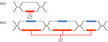
Figure 1: Schematic for the layout of an MZI and an MZL. The MZI has a single modulator, shown as a red rectangle. In the MZL we have multiple modulators, all controlled by the same drive signal. The modulators can have different lengths and so can impart different but proportional phase shifts. Blue rectangles imply independent and static programmable phase shifts.

An electro-optic modulator within a Mach–Zehnder interferometer (MZI) is a typical construction for an optical switch. Because MZIs do not rely on moving parts or resonance effects, such as for microelectromechanical systems (MEMS) or ring resonator based switches, they offer reliable, high speed operation and good thermal stability. However, any noise in the signal which drives the modulator will cause imperfect switching, which leads to optical crosstalk. Reducing this crosstalk is important for many applications. To keep communication errors in optical switching networks constant, optical crosstalk must be lower than the worst case loss Chan et al. (2008). As the complexity of optical switching networks increases, the worst case loss of the switch will increase, meaning that the allowable crosstalk for each switch decreases. Whilst intelligently designed driving electronics can reduce the noise of the drive signals, commonly occurring issues such as interference from switch mode power supplies (for example those used for temperature stabilisation) and intersymbol interference remain challenging to suppress. Because of these kinds of engineering challenges, noise in the electrical signals which drive electro-optic modulators has been identified as a key issue in realising large scale optical switching networks for classical computing applications Campenhout et al. (2009). In quantum communication schemes, intersymbol interference effects have been highlighted as a potential security flaw in integrated photonic quantum communication systems Vaquero-Stainer et al. (2018). Drive-noise is also identified as the expected dominant source of stochastic noise in LOQC Rudolph (2017). In quantum error correction codes, the error thresholds depend on both stochastic error and photon loss. Importantly, this means that any improvement to stochastic error rates will allow for more relaxed requirements on photon loss Barrett and Stace (2010).

In an ideal perfectly balanced MZI, the phase shift imparted on the switched optical modes does not depend on the phase shift imparted by the modulator. This is not true in general when unbalanced couplers are used. Many applications of optical switching use the phase of the switched optical modes to carry information, such as phase-shift keying communication schemes Xu et al. (2004) and multiplexing of entangled photonic state generation. Therefore, such phase shifts from an optical switch can be problematic. However, for applications where the phase of an optical mode does not carry information, for example in pulse amplitude modulation communications schemes and photon source multiplexing, a noisy phase shift has no impact on performance. This application dependent difference motivates us to use two fidelity measures (defined in section III) to assess the performance of our devices, one which is sensitive to phase errors and one which is not.

In an effort to solve the issues caused by drive-noise, designs have been proposed Campenhout et al. (2009) and realised Campenhout et al. (2011) for multi-stage Mach–Zehnder interferometers, known as a Mach–Zehnder lattices (MZL). These devices exhibit excellent drive-noise tolerance in their on state when assessed using phase insensitive measures. An important part of the design of these devices is that the modulation at every stage is controlled by the same drive signal, as depicted in Figure 1. One way to interpret the mechanism behind their drive-noise tolerance is that by driving multiple modulators with the same signal, the same random error due to drive-noise is applied multiple times, such that it can be thought of as a coherent, systematic error. The additional stages of the MZL can then be used to engineer some amount of cancellation of these systematic errors. An issue with existing device designs Campenhout et al. (2009, 2011) is that they impart drive-noise dependent phase shifts (see appendix A).

In this work we extend the function of existing device designs to create devices which achieve drive-noise tolerance in both their on and off state. Some of our proposed devices additionally have the property that they do not impart drive-noise dependent phase shifts on to the switched light modes. Our designs are inspired by composite pulse sequences, a technique originally created for correcting systematic errors which arise in Nuclear Magnetic Resonance.

II Composite pulses

Nuclear Magnetic Resonance (NMR), which is the study and control of nuclear spins within molecules using static and radio frequency magnetic fields Ernst et al. (1987), has widespread applications in chemistry and biochemistry, and was also one of the first systems used for demonstrating quantum information processing (QIP) Jones and Mosca (1998); Chuang et al. (1998). A common problem arises from the radio frequency control fields, which are inhomogeneous over the ensemble of molecules in a macroscopic sample. This creates a spatially varying error in the angle of rotation of the spins, leading to loss of information in the ensemble averaged signal. A popular solution to this problem is to replace the single pulse used for a rotation with a composite pulse Levitt and Freeman (1979). Appropriately engineering the angle and axis of rotation of each pulse can successfully reduce errors. Since their first demonstration, a wide variety of composite pulse sequences have been developed, designed to correct for various types of errors Levitt (1986), and have found application in NMR QIP Cummins et al. (2003).

Composite pulse sequences perform unitary evolutions on a 2-dimensional complex vector space (e.g. a qubit), and can be applied to any other system described by such a vector space. Examples include superconducting circuits Collin et al. (2004), electron spin resonance Morton et al. (2005), photon polarisation Ardavan (2007), and atom interferometers Dunning et al. (2014). In this work, we extend these applications to optical switching, which we describe by the 2-dimensional complex vector space of the 2 electromagnetic field spatial modes of our switch.

In NMR, composite pulses are also frequently used to tackle off-resonance errors Jones and Mosca (1998), which causes a tilt in the rotation axis, as well as rotation angle errors, but in optical switching the rotation induced by a modulator is confined to the $z$-axis and so tilt errors are not a significant problem.

III Device model

For simplicity, and to stay platform agnostic, we use an idealised model. All devices discussed in this work are built from directional couplers $\bm{C}(\gamma)$, fixed phase shifts $\bm{P}(\phi)$, and modulators $\bm{M}(s,\theta)$, which we define as unitary matrices that act on the 2-dimensional complex space of the amplitudes of the electromagnetic field modes

$$\bm{C}(\gamma)=\begin{pmatrix}\cos\gamma/2&-{\mathrm{i}}\sin\gamma/2\\ -{\mathrm{i}}\sin\gamma/2&\cos\gamma/2\end{pmatrix},$$ (1)

$$\bm{P}(\phi)=\begin{pmatrix}\exp({-\mathrm{i}}\phi/2)&0\\ 0&\exp({\mathrm{i}}\phi/2)\end{pmatrix},$$ (2)

$$\bm{M}(s,\theta)=\begin{pmatrix}1&0\\ 0&\exp({\mathrm{i}}\theta s)\end{pmatrix}.$$ (3)

The coupler is described by an angle, $\gamma$, which can be controlled through the physical parameters for each instance of the device. In integrated directional couplers, these parameters are typically the strength of the evanescent coupling between waveguides and the length of the coupling region.

A fixed phase shift of angle $\phi$, is implemented by creating a difference between the two optical path lengths of the two optical modes. This could be implemented using a slow precise modulator, for example using the thermo-optic effect.

We assume that all the fast electro-optic modulators within an MZL switch are controlled by the same drive signal. This allows us to model the driving signal using a single parameter, $s$, which we assume takes the same value for all the modulators at any given point in time. We define our devices such that $s=0$ describes the ideal off state and $s=1$ describes the ideal on state, and will consider the effects of small deviations from these ideal values. The on state phase shift angle of each modulator, $\theta$, can be controlled by changing the length of the modulator. To ensure the validity of this model, it is important that any other noise sources have a much smaller effect than the noise from the drive signal.

For later sections, we will also use the Hadamard transformation, which we can express, up to a global phase, as

$$\bm{H}=\bm{P}\left(\frac{\pi}{2}\right)\bm{C}\left(\frac{\pi}{2}\right)\bm{P}\left(\frac{\pi}{2}\right)=\frac{1}{\sqrt{2}}\begin{pmatrix}1&1\\ 1&-1\end{pmatrix}.$$ (4)

With these definitions, we can define an MZL switch by a sequence of these transformations. Our target transfer matrices which we will use as comparison for our fidelity measures are

$$V_{\textit{off}}=\begin{pmatrix}1&0\\ 0&1\end{pmatrix},\quad V_{\textit{on}}=\begin{pmatrix}0&1\\ 1&0\end{pmatrix}.$$ (5)

For later comparisons, we define an MZI as

$$\bm{H}\bm{M}\left(s,\pi\right)\bm{H}.$$ (6)

We only consider errors due to drive-noise, which we model as an imperfect value of $s$, meaning that we assume a linear response of our modulators and no imperfections in the passive optical devices. Although fabrication errors will introduce errors in passive optical devices, near perfect passive optical devices can be achieved for example by replacing each coupler with a Mach–Zehnder interferometer Thomas-Peter (2012); Miller (2015), then tuning it to implement the appropriate transformation $\bm{C}(\gamma)$ using either a reprogrammable Wilkes et al. (2016) or set-and-forget Chen et al. (2017); Bachman et al. (2016) phase shift. Any imbalanced losses in the devices will affect fidelity, so losses at each stage should be engineered to be balanced for any realization of these devices. Errors due to other effects such as dispersion or nonlinear effects are beyond the scope of this work.

To assess the performance of our devices, we use two different fidelity measures on the transfer matrices of our devices, $U$, against a target transfer matrix, $V$. One is a unitary fidelity measure Jones (2003)

$$F=\frac{|\operatorname{Tr}(UV^{\dagger})|^{2}}{4}$$ (7)

which is sensitive to errors in both intensity and phase. The other is a purely intensity dependent fidelity Carolan et al. (2015)

$$F_{I}=\frac{\operatorname{Tr}\left(|UV^{\dagger}|^{2}\right)}{2}$$ (8)

which is insensitive to errors in phase. Here $|A|^{2}$ indicates the elementwise absolute value squared of a matrix $A$. Determining which fidelity measure should be considered will depend on the application of interest.

IV Mapping composite pulses to optical switches

Composite pulses are described by a list of pairs of angles describing the angle of rotation, $\theta$, and the azimuthal angle of the axis of rotation in the $xy$ plane, $\phi$. Each pulse in the list is typically formatted with the angle of the axis as a subscript to the angle of rotation

$$\theta_{\phi}.$$ (9)

A subset of composite pulses known as inversion pulses are interesting in the context of optical switching as their operation corresponds to a switch in the on state as defined in equation 5. As an example, the Levitt composite inversion pulse Levitt and Freeman (1979), which we use in section V.1 is written as

$$\frac{\pi}{2}_{\frac{\pi}{2}}\,\pi_{0}\,\frac{\pi}{2}_{\frac{\pi}{2}},$$ (10)

where the angles are expressed in radians. The tolerance of rotation angle errors seen for the Levitt pulse is analogous to the refocussing of inhomogeneous broadening by spin echoes Hahn (1950) and photon echoes Abella et al. (1966).

In the photonic devices described in section III, our modulators are only able to perform $z$-axis rotations in the Bloch sphere. To translate this $z$-axis rotation to an $x$-axis rotation, we place Hadamard transformations either side of our modulators, and to control the axis of rotation in the $xy$ plane, we tilt this axis with fixed phase shifts. Finally we note that the modulator in effect performs a rotation through angle $s\theta$, and thus equation 9 becomes

$$\bm{P}\left(\phi\right)\bm{H}\bm{M}\left(s,\theta\right)\bm{H}\bm{P}\left(-\phi\right)$$ (11)

By implementing this mapping from equation 9 to equation 11 for each pulse in a sequence, we can find designs for composite pulse inspired MZL switches. These designs can then be simplified by applying the following identities:

$$\bm{P}\left(a\right)\bm{P}\left(b\right)\equiv\bm{P}\left(a+b\right)$$ (12)

$$\bm{H}\bm{P}\left(\phi\right)\bm{H}\equiv\bm{C}\left(\phi\right)\equiv\bm{P}\left(\pi\right)\bm{C}\left(-\phi\right)\bm{P}\left(\pi\right)$$ (13)

In figure 2, we show an example of applying this mapping for constructing an MZL design using the Tycko composite pulse Tycko (1983). There is some flexibility when applying the identities of equations 12 and 13, so the designer should consider what parameters they wish to optimise for. For robustness to fabrication error, each coupler, $\bm{C}$, should be replaced by two couplers and a fixed phase shift as proposed in Thomas-Peter (2012); Miller (2015).

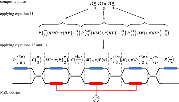
Figure 2: Outline of procedure for mapping a Tycko composite pulse Tycko (1983) to an MZL switch design. Red rectangles represent the modulators, $\bm{M\left(s,\theta\right)}$, and blue rectangles represent static phase shifts, $\bm{P}\left(\phi\right)$. If we ignore global phases, the static phase shifts $\bm{P}\left(\phi\right)$ can be implemented by acting a phase shift on only the upper mode.

In the next section, we look at the properties of MZL switches which have been designed using this mapping.

V MZL designs from known composite pulses

In this section, we show how mapping different composite inversion pulses to MZL switches can achieve switching with a range of different regimes of drive-noise tolerance. An important metric we will use to assess our devices is how successfully these composite pulse sequences can remove errors in the Taylor series expansion of the fidelity. Composite pulses can remove some of the low order terms which take the fidelity away from unity. If we first look at a conventional MZI, as defined by equation 6, we get the same expression for both our fidelity measures. The Taylor series of fidelity against the ideal on state around $s=1$ gives

$$F=F_{I}=1-\varepsilon^{2}-O\left(\varepsilon^{4}\right),$$ (14)

where we have defined $\varepsilon=\pi(s-1)/2$. When we look at off state fidelity we instead use $\varepsilon=\pi s/2$. If we compare this to the Levitt composite NOT pulse sequence Levitt and Freeman (1979), the first known composite pulse, we find that $F$ is the same as for the MZI, but the intensity only fidelity measure for the on state gives

$$F_{I}=1-\varepsilon^{4}-O\left(\varepsilon^{6}\right).$$ (15)

So for the Levitt pulse, we can say that the leading term in the expansion in the on state of $F$ is $\varepsilon^{2}$ and for $F_{I}$ is $\varepsilon^{4}$.

Another important parameter for us to keep track of is the modulation depth. This quantity is proportional to the total length of the modulators that the light will propagate through. We define modulation depth as

$$D=\frac{1}{\pi}\sum_{i}\theta_{i}$$ (16)

where $\theta_{i}$ gives the length of the $i$th modulator as defined in equation 3, which means that $D=1$ for an MZI.

A description of the Levitt pulse and all other pulses in this text as both composite pulse sequences and MZL switches can be found in appendix B.

V.1 On state drive-noise tolerance

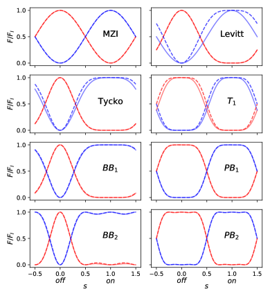
Figure 3: $F$ (solid) and $F_{I}$ (dashed) plotted for all the optical switch designs discussed in section V when compared to the ideal off state (red) and on state (blue).

		leading infidelity term
Device	D	on state		off state
		$F$	$F_{I}$	$F$	$F_{I}$
MZI	1	$\varepsilon^{2}$	$\varepsilon^{2}$	$\varepsilon^{2}$	$\varepsilon^{2}$
Levitt	2	$\varepsilon^{2}$	$\varepsilon^{4}*$	$2\varepsilon^{2}$	$2\varepsilon^{2}$
Tycko	3	$0.75\varepsilon^{4}*$	$\varepsilon^{6}*$	$3\varepsilon^{2}$	$3\varepsilon^{2}$
T1	5	$3.75\varepsilon^{4}$	$10\varepsilon^{6}$	$3.75\varepsilon^{4}*$	$10\varepsilon^{6}*$
BB1	5	$0.625\varepsilon^{6}*$	$0.625\varepsilon^{6}$	$3.75\varepsilon^{2}$	$3.75\varepsilon^{2}$
PB1	9	$7.875\varepsilon^{6}$	$7.875\varepsilon^{6}$	$7.875\varepsilon^{6}*$	$7.875\varepsilon^{6}$

Table 1: Performance summary for devices presented in section V. An asterisk (*) is used to indicate when a pulse out-performs any pulse with smaller depth D on the measure indicated.

The Levitt pulse, discussed above, achieves improved drive-noise tolerance when measured by $F_{I}$ and has an optical depth, $D=2$. By going to larger modulation depths, we can further improve our drive-noise tolerance. For $D=3$, the Tycko pulse Tycko (1983) offers on state drive-noise tolerance in both $F$ and $F_{I}$ fidelity measures, with a leading infidelity term of $0.75\varepsilon^{4}$ for $F$ and $\varepsilon^{6}$ for $F_{I}$.

V.2 On and off state drive-noise tolerance

At a modulation depth of $D=5$, there exists an interesting composite pulse sequence, designed by Wimperis, which we refer to as T₁ Wimperis (1989). This pulse sequence is the shortest known example which is designed to have a rectangular profile, meaning that when we use it in an MZL switch, we have drive-noise tolerance in both the on and off states. The T₁ pulse has a leading infidelity term of $3.75\varepsilon^{4}$ for $F$ and $10\varepsilon^{6}$ for $F_{I}$, but unlike before, this is true in both the on and off state, as shown in Figure 3. Achieving both on and off state drive-noise tolerance is particularly important for push-pull modulation schemes. Push-pull refers to when there is a modulator on both of the paths through the interferometer and the phase shift is applied by alternating which modulator is switched on, meaning that voltage needs to be applied to the device in both the on and off states.

V.3 Increasing fidelity

To find an MZL design which can suppress the 4th order unitary infidelity terms for the on state, we again need to go up to a modulation depth, $D=5$. The broadband pulse BB₁ Wimperis (1994), designed by Wimperis, meets this criterion.

To find a pulse sequence which can suppress 4th order infidelity terms of $F$ in both the on and off state, we look to the passband pulses by Wimperis Wimperis (1994). The PB₁ pulse requires a modulation depth of $D=9$ and suppresses 2nd and 4th order terms of infidelity for $F$ and $F_{I}$ in both on and off states. The devices presented so far are summarised in Table 1.

V.4 Trading fidelity for increased tolerance

The pulses presented in sections V.1 and V.2 have been optimised for maximum fidelity in the presence of small errors due to drive-noise. However, other pulses exist which offer protection against still larger errors, but at a slightly lower fidelity for small errors. Wimperis explored this trade off and created the BB₂ and PB₂ pulse Wimperis (1994), which are related to the BB₁ and PB₁ pulses. These pulses are shown in the bottom row of Figure 3.

VI Discussion

By leveraging the mature field of composite pulses, we have shown that new regimes of drive-noise tolerance in optical switches should be possible. We present designs which achieve drive-noise tolerance without decreasing unitary fidelity and designs which show on and off state drive-noise tolerance, a goal set out in Campenhout et al. (2009). This enables high fidelity push-pull based optical switches even with a noisy drive signal. Whilst for some applications, the cost of increased complexity of using MZL switches will not justify the improvements to drive noise tolerance, we have identified several areas where drive noise tolerance is critically important and so this trade off will be worthwhile. We also believe that there may be other ways to leverage composite pulses for designing other integrated photonics devices, such as MZL broadband couplers Tormen and Cherchi (2005); Jinguji et al. (1990); Takagi et al. (1992); Lu et al. (2015) or filters Kuznetsov (1994); Horst et al. (2013); Marpaung et al. (2012).

All of the devices discussed here have been designed based on inversion pulses, but it may be interesting to look at composite pulses for other rotation angles. These might find application, for example, in drive-noise tolerant adaptive measurements of dual rail photonic qubits. The BB₁ and PB₁ pulses are easily adapted for other rotation angles Wimperis (1994), and so provide a completely general solution to this problem.

It is possible to continue suppressing further terms in the infidelity in the on state by designing MZL switches with higher modulation depth Brown et al. (2004); Jones (2013). However, we think that this trade off will not be practical due to the increased losses, footprint and power consumption associated with higher modulation depth. Also, composite pulses are designed to tackle systematic errors where the general form of the errors, but not their precise magnitude, is known, and so only work well when the dominant errors take the expected form. Simulations and experimental studies in the context of NMR Xiao and Jones (2006); Kabytayev et al. (2014); Zhen et al. (2016); Torosov and Vitanov (2019) suggest that composite pulses are an effective means of error suppression in many cases, but that short and simple sequences may in practice work better than more complex sequences with theoretically better performance. Although fabrication errors can be suppressed near perfectly using the techniques of Miller (2015); Thomas-Peter (2012), remaining effects due to fabrication error and error from other effects will limit the benefit of using the more complex MZL switches.

Challenges remain to realise devices which can fully capitalise on these advances. Using more realistic and platform specific models to inform fine tuning of the device designs will help to offset issues such as fabrication imperfection and loss. The designs presented require precise control over many internal phase shifts within the device. If this is to be achieved using tuning or trimming, it presents a calibration challenge. It may be required to monitor transmission of light at each stage of the MZL, through a process similar to proposals for calibrating passive MZL filters Miller (2017). Options to achieve this include weakly coupled integrated detectors, “taps” to route some of the light to external detectors or frequency selective Bragg gratings Calkins et al. (2013). To avoid increased losses, these taps could be made using a process which allows for them to be removed Topley et al. (2014). Alternatively, a modular construction Clements (2018); Mennea et al. (2018) would allow for each stage to be calibrated individually.

Appendix A Existing drive-noise tolerant MZL designs

The designs in Campenhout et al. (2009) were created by imagining taking an MZI and breaking up the modulation into $N$ smaller pieces, surrounded by $N+1$ couplers. To ensure extinction in the off state, their couplers are constrained such that

$$\sum_{i=1}^{N+1}\gamma_{i}=\pi$$ (17)

and they chose to make their devices symmetric i.e. $\gamma_{i}=\gamma_{N+1-i}$. They break up the modulator evenly, i.e. $\theta_{i}=\pi/N$. With these shorter modulators, they found that they needed to apply larger voltages to reach the on state than for a MZI. If we rescale our $s$ parameter and $\theta_{i}$ parameters such that the on state occurs at $s=1$, we find that this gives $\theta_{i}=\pi$ for all devices presented in Campenhout et al. (2009). Figure 4 shows the performance of the design from Campenhout et al. (2011), which was made using the methods in Campenhout et al. (2009), when modelled in the framework used in this work. As seen in the figure, the fidelity of these devices depends strongly on whether a phase sensitive or phase insensitive fidelity measure is used, and therefore renders these devices unsuitable for applications where phase information is important.

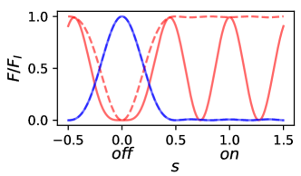
Figure 4: $F$ (solid) and $F_{I}$ (dashed) for MZL used in Campenhout et al. (2011), and designed according to the methods in Campenhout et al. (2009), when compared to the ideal off state (red) and on state (blue). Ideal on and off states for this MZL are the reverse of the convention outlined in section III.

It is worth commenting that our simplistic device model succeeds in describing the drive-noise tolerance behaviour of devices which have been experimentally realised Campenhout et al. (2011). We expect that the reverse will be true, and that the devices we present in this work will inspire real devices with enhanced drive-noise tolerance, despite our model excluding many forms of imperfections.

Appendix B Composite pulses and Mach–Zehnder Lattice designs

Table 2 shows the result of using the mapping and simplifications described in section IV, applied to the sequences discussed in this paper. Simplifications were applied to reduce the terms in the sequence, rather than to suggest the most practically appropriate design. We let $\alpha=\arccos(-1/4)$ and $\beta=\arccos(-1/8)$.

Table 2: Composite pulse sequences and MZL switch designs for all devices discussed

Design	Pulse sequence	MZL switch design
MZI	$\pi_{0}$	$\bm{H}\bm{M}\left(s,\pi\right)\bm{H}$
Levitt	$\frac{\pi}{2}_{\frac{\pi}{2}}\pi_{0}\frac{\pi}{2}_{\frac{\pi}{2}}$	$\bm{P}\left(\frac{\pi}{2}\right)\bm{H}\bm{M}\left(s,\frac{\pi}{2}\right)\bm{C}\left(-\frac{\pi}{2}\right)\bm{M}\left(s,\pi\right)\bm{C}\left(\frac{\pi}{2}\right)\bm{M}\left(s,\frac{\pi}{2}\right)\bm{H}\bm{P}\left(-\frac{\pi}{2}\right)$
Tycko	$\pi_{\frac{\pi}{3}}\pi_{\frac{5\pi}{3}}\pi_{\frac{\pi}{3}}$	$\bm{P}\left(\frac{\pi}{3}\right)\bm{H}\bm{M}\left(s,\pi\right)\bm{C}\left(\frac{4\pi}{3}\right)\bm{M}\left(s,\pi\right)\bm{C}\left(-\frac{4\pi}{3}\right)\bm{M}\left(s,\pi\right)\bm{H}\bm{P}\left(-\frac{\pi}{3}\right)$
T1	$2\pi_{-\alpha}2\pi_{\alpha}\pi_{0}$	$\bm{P}\left(\alpha\right)\bm{H}\bm{M}\left(s,2\pi\right)\bm{C}\left(2\alpha\right)\bm{M}\left(s,2\pi\right)\bm{C}\left(-\alpha\right)\bm{M}\left(s,\pi\right)\bm{H}$
BB1	$\pi_{\alpha}2\pi_{3\alpha}\pi_{\alpha}\pi_{0}$	$\bm{P}\left(\alpha\right)\bm{H}\bm{M}\left(s,\pi\right)\bm{C}\left(2\alpha\right)\bm{M}\left(s,2\pi\right)\bm{C}\left(-2\alpha\right)\bm{M}\left(s,\pi\right)\bm{C}\left(-\alpha\right)\bm{M}\left(s,\pi\right)\bm{H}$
PB1	$2\pi_{\beta}4\pi_{-\beta}2\pi_{\beta}\pi_{0}$	$\bm{P}\left(\beta\right)\bm{H}\bm{M}\left(s,2\pi\right)\bm{C}\left(-2\beta\right)\bm{M}\left(s,4\pi\right)\bm{C}\left(2\beta\right)\bm{M}\left(s,2\pi\right)\bm{C}\left(-\beta\right)\bm{M}\left(s,\pi\right)\bm{H}$
BB2	$\pi_{\frac{\pi}{2}}2\pi_{-\frac{\pi}{4}}\pi_{\frac{\pi}{2}}\pi_{0}$	$\bm{P}\left(\frac{\pi}{2}\right)\bm{H}\bm{M}\left(s,\pi\right)\bm{C}\left(-\frac{3\pi}{4}\right)\bm{M}\left(s,2\pi\right)\bm{C}\left(\frac{3\pi}{4}\right)\bm{M}\left(s,\pi\right)\bm{C}\left(-\frac{\pi}{2}\right)\bm{M}\left(s,\pi\right)\bm{H}$
PB2	$2\pi_{\frac{\pi}{2}}4\pi_{-\frac{5\pi}{8}}2\pi_{\frac{\pi}{2}}\pi_{0}$	$\bm{P}\left(\frac{\pi}{2}\right)\bm{H}\bm{M}\left(s,2\pi\right)\bm{C}\left(\frac{7\pi}{8}\right)\bm{M}\left(s,4\pi\right)\bm{C}\left(-\frac{7\pi}{8}\right)\bm{M}\left(s,2\pi\right)\bm{C}\left(-\frac{\pi}{2}\right)\bm{M}\left(s,\pi\right)\bm{H}$

References

- Campenhout et al. (2009) J. V. Campenhout, W. M. J. Green, and Y. A. Vlasov, Opt. Express 17, 23793 (2009).
- Shacham et al. (2008) A. Shacham, K. Bergman, and L. P. Carloni, IEEE Trans. Comput. 57, 1246 (2008).
- Sun et al. (2015) C. Sun, M. T. Wade, Y. Lee, J. S. Orcutt, L. Alloatti, M. S. Georgas, A. S. Waterman, J. M. Shainline, R. R. Avizienis, S. Lin, B. R. Moss, R. Kumar, F. Pavanello, A. H. Atabaki, H. M. Cook, A. J. Ou, J. C. Leu, Y.-H. Chen, K. Asanović, R. J. Ram, M. A. Popović, and V. M. Stojanović, Nature 528, 534 (2015).
- Miller (2009) D. A. B. Miller, Proc. IEEE 97, 1166 (2009).
- Cheng et al. (2018) Q. Cheng, M. Bahadori, M. Glick, S. Rumley, and K. Bergman, Optica 5, 1354 (2018).
- Monroe et al. (2014) C. Monroe, R. Raussendorf, A. Ruthven, K. R. Brown, P. Maunz, L.-M. Duan, and J. Kim, Phys. Rev. A 89, 022317 (2014).
- Nickerson et al. (2014) N. H. Nickerson, J. F. Fitzsimons, and S. C. Benjamin, Phys. Rev. X 4, 041041 (2014).
- Choi et al. (2019) H. Choi, M. Pant, S. Guha, and D. Englund, npj Quantum Inf. 5, 1 (2019).
- Knill et al. (2001) E. Knill, R. Laflamme, and G. J. Milburn, Nature 409, 46 (2001).
- Kok et al. (2007) P. Kok, W. J. Munro, K. Nemoto, T. C. Ralph, J. P. Dowling, and G. J. Milburn, Rev. Mod. Phys. 79, 135 (2007).
- Rudolph (2017) T. Rudolph, APL Photonics 2, 030901 (2017), https://doi.org/10.1063/1.4976737 .
- Bonneau et al. (2015) D. Bonneau, G. J. Mendoza, J. L. O’Brien, and M. G. Thompson, New J. Phys. 17, 043057 (2015).
- Li et al. (2015) Y. Li, P. C. Humphreys, G. J. Mendoza, and S. C. Benjamin, Phys. Rev. X 5, 041007 (2015).
- Gimeno-Segovia (2015) M. Gimeno-Segovia, Towards practical linear optical quantum computing, Ph.D. thesis, Department of Physics, Imperial College London (2015).
- Silverstone et al. (2016) J. W. Silverstone, D. Bonneau, J. L. O’Brien, and M. G. Thompson, IEEE J. Sel. Top. Quantum Electron. 22, 390 (2016).
- Wang et al. (2018) C. Wang, M. Zhang, X. Chen, M. Bertrand, A. Shams-Ansari, S. Chandrasekhar, P. Winzer, and M. Lončar, Nature 562, 101 (2018).
- Alexander et al. (2018) K. Alexander, J. P. George, J. Verbist, K. Neyts, B. Kuyken, D. Van Thourhout, and J. Beeckman, Nat. Commun. 9, 3444 (2018).
- Carolan et al. (2015) J. Carolan, C. Harrold, C. Sparrow, E. Martín-López, N. J. Russell, J. W. Silverstone, P. J. Shadbolt, N. Matsuda, M. Oguma, M. Itoh, G. D. Marshall, M. G. Thompson, J. C. F. Matthews, T. Hashimoto, J. L. O’Brien, and A. Laing, Science 349, 711 (2015).
- Stabile et al. (2012) R. Stabile, A. Albores-Mejia, and K. A. Williams, Opt. Lett. 37, 4666 (2012).
- He et al. (2019) M. He, M. Xu, Y. Ren, J. Jian, Z. Ruan, Y. Xu, S. Gao, S. Sun, X. Wen, L. Zhou, et al., Nat. Photonics 13, 359 (2019).
- Li et al. (2018) Q. Li, J.-H. Han, C. P. Ho, S. Takagi, and M. Takenaka, Opt. Express 26, 35003 (2018).
- Chan et al. (2008) J. Chan, A. Biberman, B. G. Lee, and K. Bergman, LEOS 2008 - 21st Annual Meeting of the IEEE Lasers and Electro-Optics Society , 300 (2008).
- Vaquero-Stainer et al. (2018) A. Vaquero-Stainer, R. A. Kirkwood, V. Burenkov, C. J. Chunnilall, A. G. Sinclair, A. Hart, H. Semenenko, P. Sibson, C. Erven, and M. G. Thompson, Quantum Technologies 2018 10674, 145 (2018).
- Barrett and Stace (2010) S. D. Barrett and T. M. Stace, Phys. Rev. Lett. 105, 200502 (2010).
- Xu et al. (2004) C. Xu, X. Liu, and X. Wei, IEEE J. Sel. Top. Quantum Electron. 10, 281 (2004).
- Campenhout et al. (2011) J. V. Campenhout, W. M. J. Green, S. Assefa, and Y. A. Vlasov, Opt. Express 19, 11568 (2011).
- Ernst et al. (1987) R. R. Ernst, G. Bodenhausen, and A. Wokaun, Principles of Nuclear Magnetic Resonance in One and Two Dimensions (Oxford University Press, 1987).
- Jones and Mosca (1998) J. A. Jones and M. Mosca, J. Chem. Phys. 109, 1648 (1998).
- Chuang et al. (1998) I. L. Chuang, L. M. K. Vandersypen, X. Zhou, D. W. Leung, and S. Lloyd, Nature 393, 143 (1998).
- Levitt and Freeman (1979) M. H. Levitt and R. Freeman, J. Magn. Reson. 33, 473 (1979).
- Levitt (1986) M. H. Levitt, Prog. NMR Spectrosc. 18, 61 (1986).
- Cummins et al. (2003) H. K. Cummins, G. Llewellyn, and J. A. Jones, Phys. Rev. A 67, 042308 (2003).
- Collin et al. (2004) E. Collin, G. Ithier, A. Aassime, P. Joyez, D. Vion, and D. Esteve, Phys. Rev. Lett. 93, 157005 (2004).
- Morton et al. (2005) J. J. L. Morton, A. M. Tyryshkin, A. Ardavan, K. Porfyrakis, S. A. Lyon, and G. A. D. Briggs, Phys. Rev. Lett 95, 200501 (2005).
- Ardavan (2007) A. Ardavan, New J. Phys. 9, 24 (2007).
- Dunning et al. (2014) A. Dunning, R. Gregory, J. Bateman, N. Cooper, M. Himsworth, J. A. Jones, and T. Freegarde, Phys. Rev. A 90, 033608 (2014).
- Thomas-Peter (2012) N. Thomas-Peter, Quantum-Enhanced Precision Measurement and Information Processing with Integrated Photonics, Ph.D. thesis, Clarendon Laboratory, University of Oxford (2012).
- Miller (2015) D. A. B. Miller, Optica 2, 747 (2015).
- Wilkes et al. (2016) C. M. Wilkes, X. Qiang, J. Wang, R. Santagati, S. Paesani, X. Zhou, D. A. B. Miller, G. D. Marshall, M. G. Thompson, and J. L. O’Brien, Opt. Lett. 41, 5318 (2016).
- Chen et al. (2017) X. Chen, M. M. Milosevic, D. J. Thomson, A. Z. Khokhar, Y. Franz, A. F. J. Runge, S. Mailis, A. C. Peacock, and G. T. Reed, Photon. Res. 5, 578 (2017).
- Bachman et al. (2016) D. Bachman, Z. Chen, Y. Y. Tsui, R. Fedosejevs, and V. Van, 2016 Optical Fiber Communications Conference and Exhibition (OFC) , 1 (2016).
- Jones (2003) J. A. Jones, Phys. Rev. A 67, 012317 (2003).
- Hahn (1950) E. L. Hahn, Phys. Rev. 80, 580 (1950).
- Abella et al. (1966) I. D. Abella, N. A. Kurnit, and S. R. Hartmann, Phys. Rev. 141, 391 (1966).
- Tycko (1983) R. Tycko, Phys. Rev. Lett. 51, 775 (1983).
- Wimperis (1989) S. Wimperis, J. Magn. Reson. 83, 509 (1989).
- Wimperis (1994) S. Wimperis, J. Magn. Reson. A 109, 221 (1994).
- Tormen and Cherchi (2005) M. Tormen and M. Cherchi, J. Light. Technol. 23, 4387 (2005).
- Jinguji et al. (1990) K. Jinguji, N. Takato, A. Sugita, and M. Kawachi, Electron. Lett. 26, 1326 (1990).
- Takagi et al. (1992) A. Takagi, K. Jinguji, and M. Kawachi, J. Light Technol. 10, 1814 (1992).
- Lu et al. (2015) Z. Lu, H. Yun, Y. Wang, Z. Chen, F. Zhang, N. A. F. Jaeger, and L. Chrostowski, Opt. Express 23, 3795 (2015).
- Kuznetsov (1994) M. Kuznetsov, J. Light. Technol. 12, 226 (1994).
- Horst et al. (2013) F. Horst, W. M. Green, S. Assefa, S. M. Shank, Y. A. Vlasov, and B. J. Offrein, Opt. Express 21, 11652 (2013).
- Marpaung et al. (2012) D. Marpaung, C. Roeloffzen, R. Heideman, A. Leinse, S. Sales, and J. Capmany, Laser Photonics Rev. 7, 506 (2012).
- Brown et al. (2004) K. R. Brown, A. W. Harrow, and I. L. Chuang, Phys. Rev. A 70, 052318 (2004).
- Jones (2013) J. A. Jones, Phys. Lett. A 377, 2860 (2013).
- Xiao and Jones (2006) L. Xiao and J. A. Jones, Phys. Rev. A 73, 032334 (2006).
- Kabytayev et al. (2014) C. Kabytayev, T. J. Green, K. Khodjasteh, M. J. Biercuk, L. Viola, and K. R. Brown, Phys. Rev. A 90, 012316 (2014).
- Zhen et al. (2016) X.-L. Zhen, T. Xin, F.-H. Zhang, and G.-L. Long, Sci. China Phys. Mech. 59, 690312 (2016).
- Torosov and Vitanov (2019) B. T. Torosov and N. V. Vitanov, Phys. Rev. A 100, 023410 (2019).
- Miller (2017) D. A. B. Miller, Opt. Express 25, 29233 (2017).
- Calkins et al. (2013) B. Calkins, P. L. Mennea, A. E. Lita, B. J. Metcalf, W. S. Kolthammer, A. Lamas-Linares, J. B. Spring, P. C. Humphreys, R. P. Mirin, J. C. Gates, P. G. R. Smith, I. A. Walmsley, T. Gerrits, and S. W. Nam, Opt. Express 21, 22657 (2013).
- Topley et al. (2014) R. Topley, G. Martinez-Jimenez, L. O’Faolain, N. Healy, S. Mailis, D. J. Thomson, F. Y. Gardes, A. C. Peacock, D. N. R. Payne, G. Z. Mashanovich, and G. T. Reed, Proc. SPIE 8990, 899008 (2014).
- Clements (2018) W. Clements, Linear Quantum Optics: Components and Applications, Ph.D. thesis, Clarendon Laboratory, University of Oxford (2018).
- Mennea et al. (2018) P. L. Mennea, W. R. Clements, D. H. Smith, J. C. Gates, B. J. Metcalf, R. H. S. Bannerman, R. Burgwal, J. J. Renema, W. S. Kolthammer, I. A. Walmsley, and P. G. R. Smith, Optica 5, 1087 (2018).