An anytime tree search algorithm for the 2018 ROADEF/EURO challenge glass cutting problem

Abstract

In this article, we present the anytime tree search algorithm we designed for the 2018 ROADEF/EURO challenge glass cutting problem proposed by the French company Saint-Gobain. The resulting program was ranked first among 64 participants. Its key components are: a new search algorithm called Memory Bounded A* (MBA*) with guide functions, a symmetry breaking strategy, and a pseudo-dominance rule. We perform a comprehensive study of these components showing that each of them contributes to the algorithm global performances. In addition, we designed a second tree search algorithm fully based on the pseudo-dominance rule and dedicated to some of the challenge instances with strong precedence constraints. On these instances, it finds the best-known solutions very quickly.

We present the algorithm that allowed us to win the final phase of the 2018 ROADEF/EURO challenge.

We introduce a new generic anytime tree search algorithm called Memory Bounded A*.

We outline guide functions, a symmetry breaking strategy, and a pseudo-dominance rule.

We show by a comprehensive study that each of these components contributes to the algorithm global performance.

We describe another tree search algorithm fully based on the pseudo-dominance rule and dedicated to instances with strong precedence constraints, for which it quickly finds the best-known solutions

1 Introduction

In automated planning and scheduling (AI planning) communities, resolution methods often involve exploring a search tree. These methods usually perform an advanced greedy procedure. They explore the search tree starting with the parts that are evaluated a priori most promising and continue the exploration (so long as computational time is provided). Such methods are called anytime tree searches because they can be stopped at any time and provide good solutions relatively to the allowed computation time. Thus, they share the same purpose as classical meta-heuristics, but are less common in Operations Research. Still, one called Beam Search has shown a relative popularity in the Cutting & Packing literature (Akeb et al., 2009; Bennell and Song, 2010; Baldi et al., 2014). They usually perform little inference within each node, and thus can open millions of nodes per second.

On the other hand, branch & bound algorithms are ubiquitous in Operations Research. Such methods are usually designed to prove optimality, thus relying on strong bound computations (such as Lagrangian relaxations) and advanced pruning rules (dominances, symmetries, etc.) to reduce the size of the search tree as much as possible. However, such refined computations often drastically reduce the number of nodes opened per second. Consequently, the quality of solutions obtained on larger instances can be harmed due to fewer nodes opened.

The constructive nature of both anytime tree search algorithms and branch & bounds suggests that it could be possible to incorporate their respective advantages in a common approach. Indeed, some branch & bound components may be (relatively) inexpensive to compute while still greatly reducing the search space. Using them within an anytime tree search algorithm would allow getting the best of both methods. It would provide a constructive method that is designed to find good solutions fast while taking advantage of the search space reductions from branch & bounds.

With this in mind, we decided to develop such an algorithm for the 2018 ROADEF/EURO challenge glass cutting problem. We may note that this is unusual as almost all top-ranked methods in previous editions of the challenge mainly rely on local search or mathematical programming techniques.

We propose an anytime tree search with some simple bounds, pseudo-dominance properties, and symmetry breaking rules. We introduce some new guidance strategy that allows the algorithm to perform significantly better than if it was guided by a bound as in classical branch & bound methods.

The search strategy can be roughly described as follows. It is a restarting strategy that starts its first iteration by performing very aggressive heuristic prunings. At the second iteration, it performs less aggressive heuristic prunings, taking more time than the previous iteration, but finding better solutions. If the algorithm runs long enough, some iteration may perform no heuristic pruning, thus the method will be able to guarantee optimality. The resulting method obtained the best results compared to the other submitted approaches during the final phase. We named it Memory Bounded A* as it performs a series of A* with heuristic prunings which guarantee no-more than a given amount of nodes active at the same time.

We also highlight a general methodology that can be applied to other complex problems (and with other tree search algorithms). Indeed, the method can be divided into two parts: the Branching Scheme, usually problem-specific, which is a definition of the implicit search tree (i.e.  root node, how to generate children of a given node, lower bounds, dominance rules, etc.); and a strategy, usually generic, to explore the tree. This decomposition allows rapid prototyping of both search tree definitions and tree search algorithms as many generic parts can be reused within other algorithms. It also helps to draw insights about the contribution of each component to the resulting search algorithm.

This paper is structured as follows. In Section 2, we state the problem constraints and objective. In Section 3, we give some notations and definitions. In Section 4, we describe the branching scheme and in Section 5, the tree search algorithm we designed. Finally, in Section 6, we show the numerical results we obtained.

2 Problem description

The 2018 ROADEF/EURO challenge was dedicated to an industrial cutting problem from the French company Saint-Gobain. The challenge consists in packing rectangular glass items into standardized bins of dimensions $W\times H$ (6m $\times$ 3.21m).

The cutting plan needs to satisfy the following constraints:

• All items need to be produced

• Item rotation is allowed

• Cuts must be of guillotine type. Figure 1 illustrates two examples of non-guillotine and guillotine patterns. Furthermore, the number of stages is limited to four, with only one $4$-cut allowed on a sub-plate obtained after $3$-cuts. This configuration is close to classical three-staged non-exact guillotine patterns, but differs in that a sub-plate obtained after $3$-cuts may contain two items as illustrated in Figure 2.

  

  (a) Non-guillotine pattern

  

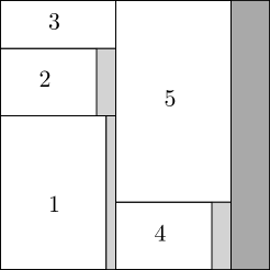
  (b) Guillotine pattern

  Figure 1: Illustration of a non-guillotine pattern (a) and a guillotine one (b)

  (a)

  (b)

  Figure 2: Only one $4$-cut is allowed. Therefore, pattern (a) is feasible but pattern (b) is not

• Items are subject to chain precedence constraints. The extraction order is as follows: rightmost first level sub-plates first; within a first level sub-plate, bottommost second level sub-plates first; within a second level sub-plate, rightmost items first; and within a third level sub-plate, bottommost item first. Most instances have a dozen chains, three instances have $2$ chains and five instances are not subject to precedence constraints.

• Bins contain defects (between $0$ and $8$ rectangles about a few centimeters high and wide). Items must be defect-free and it is forbidden to cut through a defect. Even if the bins have the same dimensions, the presence of defects makes the set of bins heterogenous. It is important to note that bins must be used in the order they are given.

• Depending on their level, sub-plates are subject to minimum and maximum size constraints. The width of first level sub-plates must lie between $w_{\text{min}}^{1}=100$ and $w_{\text{max}}^{1}=3500$, except for wastes. The height of second-level sub-plates must be at least $w_{\text{min}}^{2}=100$, except for wastes. Finally, the width and the height of any waste area must be at least $w_{\text{min}}=20$. This last constraint has an unusual consequence as illustrated in Figure 3.

The objective is to minimize the total waste area. It differs from classical Bin Packing Problems in that the remaining part of the last bin is not counted as waste. This objective is known in the packing literature as Bin Packing with Leftovers. It can be formulated as:

$$\min\;\;\;nHW-Hw-\sum_{i\in\mathcal{I}}w_{i}h_{i}$$

where $n$ is the number of bins used; $W$ and $H$ are respectively the standardized width and height of the bins; $w$ is the position of the last $1$-cut; $\mathcal{I}$ is the set of produced items; and $w_{i}$ and $h_{i}$ are respectively the width and the height of item $i\in\mathcal{I}$.

Figure 3: Optimal solution of the case containing the following three items with the chain precedence constraint $J_{1}\to J_{2}\to J_{3}$. Additional waste must be added before the first $1$-cut. Otherwise either the waste area to the right of $J_{1}$ or the waste area to the right of $J_{2}$ would violate the minimum waste constraint.

3 Definitions and notations

We use the following vocabulary: a $k$-cut is a cut performed in the $k$-th stage. Cuts separate bins or sub-plates in $k$-th level sub-plates. For example, $1$-cuts separate the bin in several first level sub-plates. $S$ denotes a solution or a node in the search tree.

We call the last first level sub-plate, the rightmost one containing an item; the last second level sub-plate, the topmost one containing an item in the last first level sub-plate; and the last third level sub-plate the rightmost one containing an item in the last second level sub-plate. $x_{1}^{\text{prev}}(S)$ and $x_{1}^{\text{curr}}(S)$ are the left and right coordinates of the last first level sub-plate; $y_{2}^{\text{prev}}(S)$ and $y_{2}^{\text{curr}}(S)$ are the bottom and top coordinates of the last second level sub-plate; and $x_{3}^{\text{prev}}(S)$ and $x_{3}^{\text{curr}}(S)$ are the left and right coordinates of the last third level sub-plate. Figure 4 presents a usage example of these definitions. We define the area and the waste of a solution $S$ as follows:

To compute $\mathrm{area}(S)$ we distinguish two cases

• if $S$ contains all items:

  $$\mathrm{area}(S)=x_{1}^{\text{curr}}(S)h$$

• and otherwise:

  $$\mathrm{area}(S)=\begin{array}[]{lll}A&+&x_{1}^{\text{prev}}(S)h\\ &+&(x_{1}^{\text{curr}}(S)-x_{1}^{\text{prev}}(S))y_{2}^{\text{prev}}(S)\\ &+&(x_{3}^{\text{curr}}(S)-x_{1}^{\text{prev}}(S))(y_{2}^{\text{curr}}(S)-y_{2}^{\text{prev}}(S))\\ \end{array}$$

We compute the waste of a partial solution as follows:

$$\mathrm{waste}(S)=\mathrm{area}(S)-\mathrm{item\_area}(S)$$

with $A$ the sum of the areas of all but the last bin, $h$ the height of the last bin and $\mathrm{item\_area}(S)$ the sum of the area of the items of $S$. Area and waste are illustrated in Figure 4.

Figure 4: Last bin of a solution which does not contain all items. The area is the whole hatched part and the waste in the grey hatched part.

4 Branching scheme

4.1 General scheme

Two kinds of packing strategies are used in the packing literature: item-based and block-based. In item based strategies, only one item is inserted at each step, whereas in block-based strategies, multiple items are inserted. Although several researchers highlighted the benefits of block-based approaches (Bortfeldt and Jungmann, 2012; Wei et al., 2014; Lodi et al., 2017), we chose an item-based strategy. Two reasons support this choice. First, the problem has more constraints than classical packing problems from the literature. Thus, generating feasible solutions is already challenging and block-based approaches add even more complexity. Second, the benefits of the block-based approaches might be compensated by a more powerful tree search algorithm.

However, our strategy is not purely item-based: instead of packing one item at each step, we pack the next third level sub-plate. This comes from the observation that because only one $4$-cut is allowed in a third level sub-plate, a third level sub-plate has only five possible configurations; it may contain

1. exactly one item, without waste

2. exactly one item with some waste above

3. exactly one item with some waste below

4. exactly two items, without waste

5. no item, only waste

These configurations are illustrated in Figure 5. The sub-plates containing $J_{1}$ and $J_{2}$ respectively follow configurations $1$ and $2$. These are the standard configurations. Placing an item on top of the sub-plate as in configuration 3 may be necessary if it would contain a defect otherwise as $J_{3}$. Similarly, inserting only waste (configuration $5$) may also be necessary if the region contains a defect as the sub-plate containing the second defect. We do not allow directly inserting only waste in a region containing no defects. Such sub-plate may appear in a solution, as the third-level sub-plate to the right of $J_{4}$ and $J_{5}$, but it is implicitly generated when $J_{6}$ is inserted. Finally, the sub-plate containing items $J_{4}$ and $J_{5}$ corresponds to configuration $4$.

Figure 5: Illustration of third level sub-plate possible configurations. Black rectangles are defects.

Third level sub-plates are inserted in the order they are extracted. In Figure 5, this follows the numbering of the items. This ensures to never violate the precedence constraints. All items are candidates if their insertion does not lead to a precedence constraint violation.

Then, a third level sub-plate can be inserted at several depths

• depth $0$: in a new bin

• depth $1$: in a new first level sub-plate to the right of the current one

• depth $2$: in a new second-level sub-plate above the current one

• depth $3$: in the current second-level sub-plate already, to the right of the last third-level sub-plate

To reduce the size of the tree, we apply some simple pruning rules:

• if a third-level sub-plate can be inserted in the current bin, we do not consider insertions in a new bin; and if a third level sub-plate can be inserted in the current first (resp. second) level sub-plate without increasing the position of its left $1$-cut (resp. top $2$-cut), we do not consider insertions in a new first (resp. second) level sub-plate;

• If the last insertion is an empty sub-plate at depth $d$, then the next insertion must also happen at depth $d$;

• If the last insertion is a $2$-item insertion at depth $d\neq 3$, then the next insertion must be at depth $3$.

With this branching scheme, item rotation and minimum and maximum distances between cuts constraints are easy to take into account.

4.2 Pseudo-dominance rule

In this section, we describe a more sophisticated heuristic dominance rule. For a (partial) solution, we define its front as the polygonal chain

$$((x^{\text{curr}}_{1},0),(x^{\text{curr}}_{1},y^{\text{prev}}_{2}),(x^{\text{curr}}_{3},y^{\text{prev}}_{2}),$$

$$(x^{\text{curr}}_{3},y^{\text{curr}}_{2}),(x^{\text{curr}}_{1},y^{\text{curr}}_{2}),(x^{\text{curr}}_{1},h))$$

Figure 6 shows two examples of solution fronts.

Figure 6: Illustration of the front of two partial solutions

Then we say that solution $S_{1}$ dominates solution $S_{2}$ iff they contain the same items and the front of $S_{1}$ is before the front of $S_{2}$. (see Figure 7).

(a)

(b)

Figure 7: Solution (a) dominates solution (b)

If the number of possible subsets of items is small, then for a given subset, we can memorize the best front currently seen during the search and prune any new dominated node encountered. This situation occurs in instances with strong precedence constraints (i.e. two chains) and this is the strategy of the DPA* algorithm presented afterward. However, for most instances, the number of possible subsets is too large and we only use the pseudo-dominance rule among the children of a node. To compensate, an additional symmetry breaking strategy is introduced.

4.3 Symmetry breaking strategy

We designed the following symmetry breaking strategy: if they do not contain defects and can be exchanged without violating the precedence constraints, a $k$-level sub-plate is forbidden to contain an item with a smaller index than the previous $k$ level sub-plate of the same $(k-1)$-level sub-plate.

Preliminary experiments showed that applying the strategy for $k=2$ and $k=3$ yield the best results. The symmetry breaking strategy is illustrated in Figure 8.

(a)

(b)

$J_{1}$, $J_{2}\to J_{3}$

(c)

Figure 8: Illustration of the symmetry breaking strategy: pattern (a) is forbidden because the second-level sub-plates containing $J_{1}$ and $J_{2}$ can be exchanged without a feasibility issue. However, pattern (b) is allowed because of the defect and pattern (c) is also allowed because if the second-level sub-plates are exchanged, then the precedence constraint between $J_{2}$ and $J_{3}$ is violated.

It should be noted that the branching scheme is not dominant, i.e. for some instances, it may not contain an optimal solution. Likewise, the pseudo-dominance rule considers that solution $S_{1}$ dominates solution $S_{2}$ whereas no optimal solution can be reached from $S_{1}$ but one can be from $S_{2}$. More details about this are given by Fontan (2019).

5 Tree search

During our initial work on the challenge, we first explored the classical “Operations Research” optimization algorithms (local-search, evolutionary algorithms and branch and bounds). However, it seemed difficult for us to find efficient local-search or evolutionary moves, while it felt relatively natural to design constructive methods. We implemented several classical constructive algorithms: a greedy algorithm quickly providing solutions but with limited quality; a Best First (A*) algorithm returning the “optimal” one (relatively to the branching scheme) on small instances; and a Depth First struggling to improve the greedy solution.

1 fringe $\leftarrow\{\mathrm{root}\}$;

2 while $\mathrm{fringe}\neq\emptyset$ and $\mathrm{time}<\mathrm{timelimit}$ do

3       $n\leftarrow extractBest(\mathrm{fringe})$;

4       $\mathrm{fringe}\leftarrow\mathrm{fringe}\setminus\{n\}$;

5       forall  $v\in neighbours(n)$  do

6             $\mathrm{fringe}\leftarrow\mathrm{fringe}\cup\{v\}$;

7            

8       end forall

9      

10 end while

Algorithm 1 A*

We remind the pseudo-code of the A* algorithm in Algorithm 1. At each iteration, the best node is extracted from the fringe and its children are added to the fringe. As written above, our implementation of A* was able to find the optimal solutions on very small instances but was quickly running out of memory larger ones because of the size of the fringe. Therefore, we decided to heuristically prune nodes to bound the required memory. This “heuristic” algorithm performed beyond expectations and provided excellent solutions. However, it depended on the amount of memory allowed for the fringe. If this parameter is too small, the search ends quickly and not benefit from the remaining available time. If too big, the search takes more time and does not provide any solution within the time limit. To get rid of this parameter, we chose to use a restart strategy where we geometrically increase the allowed memory at each restart. The new parameter to calibrate becomes the growth factor, but we found that any value between $1.25$ and $3$ provided similar results. This simple approach provided good solutions.

Motivated by this simple but yet efficient algorithm, we investigated other anytime tree search algorithms such as beam search (Ow and Morton, 1988) and beam stack search (Zhou and Hansen, 2005). We implemented and compared them on the challenge problem. To our surprise, they did not perform as well as the previously described approach. To the best of our knowledge, this approach has not been used in the Operations Research literature before. We describe it in more detail in the next section.

5.1 Memory Bounded A* (MBA*)

A* is known to minimize the cost estimate on nodes it opens. However, it suffers from a large memory requirement since it has to store a large number of nodes in the fringe. We propose a simple but yet powerful heuristic variant of A* that cuts less promising nodes if the size of the fringe goes over a parameter $D$. We call this tree search algorithm Memory Bounded A* (MBA*). If $D=1$, it generalizes a greedy algorithm and if $D=\infty$, it generalizes A*.

The pseudo-code of MBA* is given in Algorithm 2. Only lines 8 to 11 are added compared to the A* algorithm presented in Algorithm 1. MBA* starts with a fringe containing only the root node (line 1). At each iteration, the best node is extracted from the queue (lines 3 and 4) and its children are added to the queue (lines 5 to 7). If the size of the queue goes over $D$, the worst nodes are discarded (lines 8 to 11).

1fringe $\leftarrow\{\mathrm{root}\}$;

2 while $\mathrm{fringe}\neq\emptyset$ and $\mathrm{time}<\mathrm{timelimit}$ do

3       $n\leftarrow extractBest(\mathrm{fringe})$;

4       $\mathrm{fringe}\leftarrow\mathrm{fringe}\setminus\{n\}$;

5       forall  $v\in neighbours(n)$  do

6             $\mathrm{fringe}\leftarrow\mathrm{fringe}\cup\{v\}$;

7            

8       end forall

9      while  $|\mathrm{fringe}|>D$  do

10             $n\leftarrow extractWorst(\mathrm{fringe})$;

11             $\mathrm{fringe}\leftarrow\mathrm{fringe}\setminus\{n\}$;

12            

13       end while

14      

15 end while

Algorithm 2 Memory Bounded A* (MBA*)

5.2 Guide functions

Tree search methods are dependent on well-crafted guide functions which define the meaning of best and worst nodes. Using a lower bound is common in the tree search literature. Indeed, if the objective is to prove optimality, using a lower bound as a guide function will minimize the number of opened nodes. Therefore, we first tried this approach and used the waste as a guide function. We noticed that the resulting solutions packed small items on the first plates and big items on the last ones, thus generating little waste in the beginning but a lot in the end. Globally, the solution quality was not satisfactory as illustrated in Figure 9(a).

Taking this into account, we designed new guides to balance the cost of inserting small items at the beginning of the solutions:

waste percentage (= waste / area):

compared to waste only, the waste has less impact if the solution contains larger items.

waste percentage / average area of packed items:

this guide function directly adds a reward to solutions containing large items.

The benefit of these guides is illustrated in Figure 9(b).

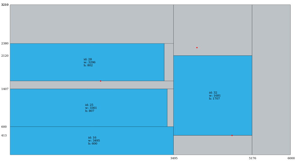
(a) waste only guide – first and last plate

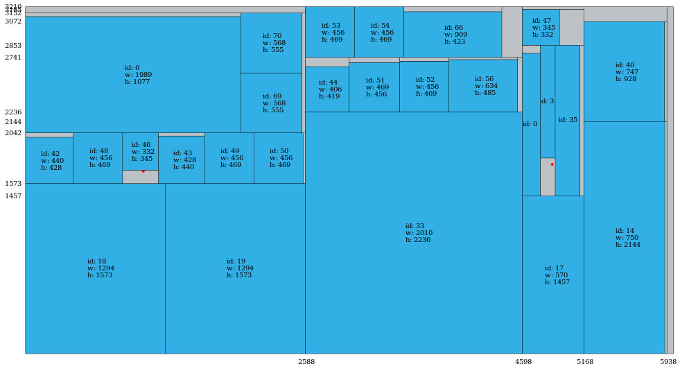
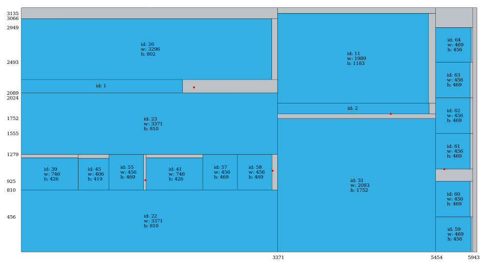
(b) waste / average size guide – first and last plate

Figure 9: 9(a) shows a solution obtained using the waste as guide function. Notice that at the beginning of the solution, small items are omnipresent whereas in later plates, only large items are present, thus globally generates more waste. 9(b) shows the effect of the guide biased by the item average size on a solution of the same instance. We observe that small and large items are better mixed and significantly less waste is generated at the end of the solution.

5.3 DPA*: solving instances with strong precedence constraints

Three instances of the challenge contain only 2 precedence chains. If we denote by $n_{1}$ (resp. $n_{2}$) the length of the first (resp. second) chain, then the number of possible subsets of items packed in a partial solution of the branching scheme becomes $n_{1}n_{2}$. Since the number of items in an instance is less than $700$ (this information was given in the challenge description), it becomes possible to store the non-dominated fronts encountered for each possible subset without overcoming the memory limitation, compare the front of each opened node with the non-dominated fronts from all the previously encountered nodes and prune the dominated ones.

Therefore, we developed a dedicated algorithm for these instances named Dynamic Programming A* (DPA*). DPA* is an A* algorithm implementing the scheme described in the previous paragraph. DPA* does not bound the size of the queue as MBA* does, and uses the waste as a guide function. Therefore, if it terminates, it returns the optimal solution (relatively to the branching scheme and the pseudo-dominance rule).

We may note that for a given subset of items, there could be an exponential number of non-dominated fronts, which could degrade DPA* performances. This is at least not an issue for the concerned instances from the challenge.

5.4 Global algorithm

For the competition, we distinguished the case where the instance has two chains or less. In this case, we run DPA*.

If it has strictly more than two chains, we do not use DPA* since it would overcome the memory limitation. Since the processor used to evaluate the participant submissions had $4$ physical cores, we run 4 threads, each one running a restarting MBA* with a given growth factor and a given guide function. Each MBA* is initially executed with a fringe maximal size of $2$, and each time one terminates, it is restarted with a maximal fringe size multiplied by its growth factor. If the growth factor is 2, the maximal size doubles at each iteration. All the threads share the information of the best solution found. If one finds a better solution, the others take advantage of it to perform more cuts and globally perform better together than alone. The threads run the following algorithms:

• MBA*, waste percentage guide, growth factor 1.33

• MBA*, waste percentage guide, growth factor 1.5

• MBA*, waste percentage / average size guide, growth factor 1.33

• MBA*, waste percentage / average size guide, growth factor 1.5

6 Numerical results

In this section, we first evaluate the contribution of the components we described in the previous sections in the main algorithm. Then, we show the benefits of using DPA* on instances with only two precedence chains. Finally, we provide computational results with the challenge setting. Instances generally have between 300 and 600 items and 10 to 15 chains. They are available online.

6.1 Contribution of the components

In this section, computational experiments have been performed on a personal computer with an Intel(R) Core(TM) i5-3470 CPU @ 3.20GHz with 16GB RAM.

We consider the $12$ possible combinations of the components we designed, namely MBA* to be compared with an Iterative Beam Search Zhang (1998); with or without the symmetry breaking strategy; and with waste (w), waste percentage (p), or waste percentage/average size (a) guide. We run each pair of instance-algorithm for $100$ seconds.

In Table 1, we show a summary of the performances of each variant. The goal is to help us select the best combinations to use. MBA* with the symmetry breaking strategy and guided by the waste percentage (MBA*+sym+p) and MBA* with the symmetry breaking strategy and guided by the waste percentage / average size (MBA*+sym+a) clearly outperform all other combinations. That is why these are the two combinations that we use. Since the processor used to evaluate participant submissions has 4 physical cores, we dedicate two threads for each combination with different growth factor (1.33 and 1.5) to add some robustness.

Combination	# best	# only best
BS+no-sym+w	2	0
BS+no-sym+p	2	0
BS+no-sym+a	2	0
BS+sym+w	5	1
BS+sym+p	9	4
BS+sym+a	9	4
MBA*+no-sym+w	2	0
MBA*+no-sym+p	3	0
MBA*+no-sym+a	4	0
MBA*+sym+w	3	0
MBA*+sym+p	23	17
MBA*+sym+a	22	18

Table 1: Comparison over all possible algorithms using the proposed algorithmic components. “# best” indicate the number of times the algorithm was able to find the best solution on given instances compared to the 11 other algorithms. “# only best” indicates the number of times the algorithm was the only one to find the best solution.

Instance	best IBS	best MBA*	best no sym	best with sym	best w	best p	best a
A1	425 486	425 486	425 486	425 486	425 486	425 486	425 486
A2	10 514 609	9 676 799	10 537 079	9 676 799	10 659 059	10 418 309	9 676 799
A3	2 651 880	2 651 880	3 441 540	2 651 880	3 056 340	2 651 880	2 651 880
A4	3 242 520	3 220 050	3 306 720	3 220 050	3 505 740	3 220 050	3 306 720
A5	3 033 273	3 566 133	4 856 553	3 033 273	3 736 263	3 033 273	3 566 133
A6	3 225 930	3 572 610	3 652 860	3 225 930	3 800 520	3 225 930	3 460 260
A7	5 063 280	4 800 060	5 194 890	4 800 060	5 933 190	4 800 060	4 938 090
A8	9 187 874	10 077 044	12 218 114	9 187 874	12 568 004	10 077 044	9 187 874
A9	2 930 706	2 985 276	3 550 236	2 930 706	3 929 016	2 930 706	2 985 276
A10	4 097 221	4 084 381	5 272 081	4 084 381	4 797 001	4 084 381	4 122 901
A11	4 718 449	4 978 459	6 076 279	4 718 449	6 711 859	5 251 309	4 718 449
A12	2 050 084	2 245 894	2 342 194	2 050 084	2 050 084	2 104 654	2 194 534
A13	15 096 453	12 133 623	14 865 333	12 133 623	15 099 663	12 197 823	12 133 623
A14	14 363 778	12 097 518	14 793 918	12 097 518	14 363 778	12 097 518	13 490 658
A15	15 277 961	13 185 041	15 168 821	13 185 041	16 029 101	13 185 041	15 014 741
A16	3 380 333	3 380 333	3 380 333	3 380 333	3 380 333	3 380 333	3 380 333
A17	3 617 251	3 617 251	3 617 251	3 617 251	3 617 251	3 617 251	3 617 251
A18	5 898 468	5 535 738	5 763 648	5 535 738	7 737 798	5 596 728	5 535 738
A19	3 323 744	3 654 374	4 187 234	3 323 744	4 620 584	3 323 744	3 965 744
A20	1 467 925	1 467 925	1 493 605	1 467 925	1 467 925	1 467 925	1 467 925
B1	4 173 228	3 633 948	4 150 758	3 633 948	4 012 728	4 324 098	3 633 948
B2	15 715 685	15 359 375	18 466 655	15 359 375	20 155 115	15 359 375	15 715 685
B3	32 668 193	21 253 433	23 365 613	21 253 433	41 315 933	24 890 363	21 253 433
B4	8 885 365	8 862 895	11 238 295	8 862 895	9 222 415	8 862 895	8 920 675
B5	92 433 185	88 590 815	88 590 815	88 590 815	103 719 545	88 590 815	88 590 815
B6	13 371 637	13 480 777	15 653 947	13 371 637	17 509 327	14 113 147	13 371 637
B7	14 576 799	11 434 209	12 801 669	11 434 209	14 319 999	11 434 209	12 801 669
B8	24 490 999	19 512 289	24 121 849	19 512 289	24 490 999	19 512 289	20 048 359
B9	20 511 607	20 046 157	25 085 857	20 046 157	46 721 257	39 071 827	20 046 157
B10	28 012 013	27 344 333	29 225 393	27 344 333	35 815 523	31 055 093	27 344 333
B11	38 143 250	29 113 520	34 175 690	29 113 520	41 523 380	32 589 950	29 113 520
B12	18 122 077	16 086 937	19 929 307	16 086 937	18 122 077	16 086 937	16 314 847
B13	31 138 545	29 674 785	33 716 175	29 674 785	31 138 545	32 213 895	29 674 785
B14	10 482 820	10 043 050	11 619 160	10 043 050	12 046 090	10 434 670	10 043 050
B15	41 533 241	28 372 241	34 143 821	28 372 241	41 533 241	28 372 241	31 466 681
X1	21 022 877	17 299 277	17 970 167	17 299 277	29 911 367	17 803 247	17 299 277
X2	11 459 837	8 583 677	8 923 937	8 583 677	9 318 767	9 206 417	8 583 677
X3	9 424 756	8 712 136	9 842 056	8 712 136	9 578 836	8 712 136	8 927 206
X4	19 035 422	15 976 292	19 305 062	15 976 292	19 035 422	15 976 292	16 772 372
X5	5 383 037	5 620 577	7 029 767	5 383 037	6 728 027	5 623 787	5 383 037
X6	14 443 523	12 167 633	14 488 463	12 167 633	14 443 523	13 024 703	12 167 633
X7	30 327 120	26 170 170	27 146 010	26 170 170	31 328 640	29 161 890	26 170 170
X8	27 693 711	27 109 491	27 693 711	27 109 491	27 693 711	27 494 691	27 109 491
X9	33 431 655	23 599 425	33 919 575	23 599 425	33 370 665	23 599 425	26 716 335
X10	23 400 722	19 901 822	23 522 702	19 901 822	23 673 572	23 975 312	19 901 822
X11	14 349 972	14 247 252	16 102 632	14 247 252	14 349 972	14 247 252	14 921 352
X12	14 775 805	12 422 875	14 576 785	12 422 875	14 775 805	12 422 875	12 589 795
X13	19 208 322	14 624 442	18 900 162	14 624 442	20 007 612	16 271 172	14 624 442
X14	11 075 552	9 730 562	11 916 572	9 730 562	11 004 932	9 730 562	10 128 602
X15	16 301 394	13 540 794	17 261 184	13 540 794	16 461 894	13 990 194	13 540 794
total waste	779 159 574	679 871 064	779 027 964	676 914 654	870 817 914	725 241 204	693 016 014
nb best	14	41	4	50	5	27	28
nb only best	9	36	0	46	1	21	22

Table 2: Analysis of the contribution of each introduced algorithmic component

Table 2 presents an analysis of the contribution of each component individually. Each column corresponds to the best result per instance obtained by a subset of algorithms that uses a given component. For instance best IBS corresponds to a subset of algorithms using Iterative Beam Search, thus excluding MBA* (6 algorithms). MBA* variants outperform the Iterative Beam Search variants (producing 12% less waste). It finds 41/50 best solutions and 36 best solutions that the Beam Search variants were not able to obtain. The algorithms using the symmetry breaking strategy clearly produce better results than the one without (13% less waste and 46 best solutions not attainable by the variants without the symmetry breaking strategy) showing that integrating state-space reductions can greatly benefit to anytime tree search algorithms and probably even to constructive meta-heuristics. Finally, as expected, the waste (lower bound) guide provides the worst results among the 3 considered guides (16% more waste than the waste percentage guide and 20% more waste than the waste percentage / average size guide and only 5 best solutions on 50 instances). However, the waste percentage guide and the waste percentage / average size guide provided similar results (with a slight advantage on the latest as it produces 5% less waste and finds one best solution more). These results are interesting as they show that both guides are complementary. Indeed, they produce 21 (resp. 22) best solutions where they are the only one to obtain them. Thus it is worth using both.

6.2 DPA*

Table 3 shows the benefits of using DPA* on instances with only two precedence chains. There is one such instance in each dataset, but the one in dataset A is trivial to solve, therefore we only consider instances B5 and X8. Unlike MBA*, DPA* is not anytime and terminates long before the $3600$ seconds time limit. Furthermore, the solutions it returns are significantly better and are even the best-known solutions for both instances.

Instance	MBA* (4 threads, 3600s)	DPA*
B5	$88\,590\,815$	$72\,155\,615$ ($2.06$s)
X8	$24\,875\,331$	$22\,265\,601$ ($59.12$s)

Table 3: DPA* vs MBA*

6.3 Final results

Table 4 sums up the challenge final results. Computational experiments have been performed on a computer with an Intel Core i7-4790 CPU @ 3.60 GHz $\times$ 8 processor with 31.3 Go of RAM. This configuration is similar to the one of the challenge. Since the challenge, a few adjustments have been made. Therefore, the results presented here slightly differ from the results obtained during the final phase. Compared to the challenge version, the current version performs better: the total waste on dataset B and X decreases from $493,600,549$ for the challenge version to $469,910,749$ for the current one. Columns Final phase best 180s and Final phase best 3600s contain the best solutions found during the final phase. Results annotated with a star indicate that this solution was found by our algorithm during the final phase of the challenge. The Best known column contains the best solution up to our knowledge. They may have been found during the development of the algorithm, with execution times exceeding $3600$ seconds or by other teams. Finally, even if it is not indicated in the table, on most of the instances, if the algorithm is run longer, for example, $2$ hours, the solution will still be improved.

Instance	Comments	Final phase best 180s	MBA*/DPA* 180s	Final phase best 3600s	MBA*/DPA* 3600s	Best known
A1	Trivial	-	425 486	-	425 486	425 486
A2	No prec	-	9 506 669	-	4 383 509	4 383 509
A3		-	2 651 880	-	2 651 880	2 651 880
A4		-	3 024 240	-	2 924 730	2 924 730
A5		-	2 924 730	-	3 283 653	3 017 223
A6		-	3 389 640	-	3 225 930	3 188 646
A7		-	4 703 760	-	4 334 610	3 920 520
A8		-	9 691 844	-	8 378 954	8 378 954
A9		-	2 664 276	-	2 664 276	2 664 276
A10		-	4 084 381	-	4 084 381	4 084 381
A11		-	4 660 669	-	4 622 149	4 358 929
A12		-	2 056 504	-	1 879 954	1 879 954
A13		-	10 226 883	-	9 440 433	9 331 293
A14		-	11 686 638	-	10 383 378	10 383 378
A15		-	12 918 611	-	11 108 171	10 828 901
A16	Trivial	-	3 380 333	-	3 380 333	3 380 333
A17	2 chains	-	3 617 251	-	3 617 251	3 617 251
A18		-	5 596 728	-	4 983 618	4 983 618
A19		-	3 654 374	-	3 323 744	3 323 744
A20	Trivial	-	1 467 925	-	1 467 925	1 467 925
B1	No prec	3 232 698	3 765 558	*2 661 318	3 136 398	2 661 318
B2		*15 635 435	14 312 915	*13 674 125	13 398 065	11 931 095
B3		20 540 813	19 786 463	18 191 093	17 093 273	15 786 803
B4		*8 269 045	8 323 615	*8 269 045	7 973 725	7 315 675
B5	2 chains	72 155 615	72 155 615	72 155 615	72 155 615	72 155 615
B6		*12 116 527	12 488 887	*11 195 257	11 089 327	10 800 427
B7	No prec	9 601 299	9 177 579	*8 355 819	7 678 509	6 628 839
B8		*17 865 559	17 152 939	16 067 959	15 840 049	14 398 759
B9		18 502 147	19 969 117	17 484 577	17 474 947	16 495 897
B10		26 012 183	26 904 563	*21 951 533	23 065 403	21 951 533
B11		25 251 890	27 312 710	22 584 380	23 820 230	20 626 280
B12		*15 868 657	13 734 007	*13 958 707	13 120 897	12 514 207
B13		*28 349 055	27 360 375	*24 471 375	23 078 235	22 657 725
B14		*9 346 480	9 442 780	*8 656 330	8 377 060	8 023 960
B15		*27 794 441	24 568 391	*24 517 031	23 088 581	22 619 921
X1		*15 508 097	15 302 657	*14 127 797	14 127 797	13 720 127
X2	No prec	6 034 937	6 083 087	*5 434 667	4 879 337	4 795 877
X3		*8 285 206	7 649 626	*7 473 076	7 180 966	6 837 496
X4		12 182 072	15 488 372	11 405 252	13 366 562	11 405 252
X5		5 081 297	4 988 207	4 712 147	4 715 357	4 522 757
X6		12 565 673	11 031 293	*10 363 613	9 496 913	9 365 303
X7		*22 443 360	22 876 710	21 127 260	21 191 460	20 568 720
X8	2 chains	*24 788 661	22 265 601	*24 788 661	22 265 601	22 265 601
X9		*22 251 225	22 312 215	20 167 935	20 479 305	20 039 535
X10		*20 110 472	18 778 322	*17 824 952	17 186 162	16 865 162
X11		*13 489 692	12 802 752	*12 417 552	11 676 042	11 011 572
X12		*11 963 845	12 358 675	*10 583 545	10 503 295	10 246 495
X13		15 950 172	14 345 172	*13 533 042	13 125 372	12 130 272
X14		*8 889 542	8 591 012	*8 013 212	7 644 062	7 422 572
X15		13 990 194	13 710 924	11 682 204	11 682 204	10 882 914

Table 4: Computational experiments comparing the proposed approach compared to other contestants

7 Conclusion and perspectives

In this article, we presented a new anytime tree search algorithm called MBA* for the 2018 ROADEF/EURO challenge glass cutting problem. It performs successive iterations, restarting when its heuristic search tree exploration is completed. During the first iterations, it performs aggressive prunings and behaves like a greedy algorithm. As iterations go, the algorithm performs fewer heuristic prunings, and thus gets access to better solutions (at the cost of an increase of the computation time of each iteration). If enough time and memory are available, the algorithm ends up performing an iteration with no heuristic pruning, finding the best solution regarding the branching scheme.

We proposed two guides (waste percentage, and waste percentage / average item size). These guides can find significantly better solutions than using a lower bound (the waste), which is what is usually used in branch and bounds. We also presented a symmetry breaking strategy and showed that it significantly improves the quality of the solutions returned by the algorithm.

Also, we designed another algorithm, DPA*, for instances with only two precedence chains. This algorithm returns the best-knowns on these instances within short times.

This result shows that anytime tree search algorithms from the AI planning community, and branch and bounds from the Operations Research community can benefit from each other, leading to algorithms competitive with classical meta-heuristics. We believe that the representation of anytime tree search algorithms in the Operations Research literature does not reflect the benefits of applying such methods on complex optimization problems. To the best of our knowledge, many of them remain unexplored such as Beam Stack Search (Zhou and Hansen, 2005), SMA* (Russell, 1992) or Anytime Column Search (Cohen et al., 2018).

Motivated by the success of MBA* on this glass cutting application, fontan2020 already adapted it for classical guillotine cutting problems from the literature and showed that even on more fundamental problems, it is still competitive with the other dedicated algorithms from the literature.

References

- Akeb et al. (2009) Akeb, H., Hifi, M., M’Hallah, R., 2009. A beam search algorithm for the circular packing problem. Computers & Operations Research 36, 1513–1528.
- Baldi et al. (2014) Baldi, M.M., Crainic, T.G., Perboli, G., Tadei, R., 2014. Branch-and-price and beam search algorithms for the variable cost and size bin packing problem with optional items. Annals of Operations Research 222, 125–141.
- Bennell and Song (2010) Bennell, J.A., Song, X., 2010. A beam search implementation for the irregular shape packing problem. Journal of Heuristics 16, 167–188.
- Bortfeldt and Jungmann (2012) Bortfeldt, A., Jungmann, S., 2012. A tree search algorithm for solving the multi-dimensional strip packing problem with guillotine cutting constraint. Annals of Operations Research 196, 53–71. URL: https://doi.org/10.1007/s10479-012-1084-7, doi:10.1007/s10479-012-1084-7.
- Cohen et al. (2018) Cohen, L., Greco, M., Ma, H., Hernández, C., Felner, A., Kumar, T.S., Koenig, S., 2018. Anytime focal search with applications., in: IJCAI, pp. 1434–1441.
- Fontan (2019) Fontan, F., 2019. Theoretical and practical contributions to star observation scheduling problems. Ph.D. thesis. URL: http://www.theses.fr/s162194. publication Title: http://www.theses.fr.
- Lodi et al. (2017) Lodi, A., Monaci, M., Pietrobuoni, E., 2017. Partial enumeration algorithms for Two-Dimensional Bin Packing Problem with guillotine constraints. Discrete Applied Mathematics 217, 40–47. URL: http://www.sciencedirect.com/science/article/pii/S0166218X15004734, doi:10.1016/j.dam.2015.09.012.
- Ow and Morton (1988) Ow, P.S., Morton, T.E., 1988. Filtered beam search in scheduling. The International Journal Of Production Research 26, 35–62.
- Russell (1992) Russell, S., 1992. Efficient memory-bounded search methods. ECAI-1992, Vienna, Austria .
- Wei et al. (2014) Wei, L., Tian, T., Zhu, W., Lim, A., 2014. A block-based layer building approach for the 2D guillotine strip packing problem. European Journal of Operational Research 239, 58–69. URL: http://www.sciencedirect.com/science/article/pii/S0377221714003464, doi:10.1016/j.ejor.2014.04.020.
- Zhang (1998) Zhang, W., 1998. Complete anytime beam search, in: AAAI/IAAI, pp. 425–430.
- Zhou and Hansen (2005) Zhou, R., Hansen, E.A., 2005. Beam-stack search: Integrating backtracking with beam search., in: ICAPS, pp. 90–98.