Stochastic modeling and estimation

of COVID-19 population dynamics

Nikolay M. Yanev

¹, Vessela K. Stoimenova², Dimitar V. Atanasov³

Abstract.

The aim of the paper is to describe a model of the development of the Covid-19 contamination of the population of a country or a region. For this purpose a special branching process with two types of individuals is considered. This model is intended to use only the observed daily statistics to estimate the main parameter of the contamination and to give a prediction of the mean value of the non-observed population of the contaminated individuals. This is a serious advantage in comparison with other more complicated models where the observed official statistics are not sufficient. In this way the specific development of the Covid-19 epidemics is considered for different countries.

2010 Mathematics Subject Classification: Primary 60J80

Secondary 60F05; 60J85; 62P10

Key words: branching processes, estimation

1. Introduction.

Nowadays the Theory of Branching Processes is a powerful tool for modeling the development of populations whose members have an ability of reproduction following some stochastic laws. The objects may be of different types and physical nature. From nuclear reaction and cosmic rays to cell proliferation and digital information, branching stochastic models are used to explain very interesting real-world stochastic phenomena. Branching processes have serious applications in Physics, Chemistry, Biology and Medicine, Demography, Epidemiology, Economics an so on. The basic models and analytical results are presented in many books and a lot of papers. We would like to point out the monographs $[1-5]$ among the others. Some applications of branching processes in Biology and Medicine are presented in $[4]$ and $[6]$.  Some basic estimation problems are considered in $[7].$

The aim of the present paper is to describe an adequate model of the development of the Covid-19 contamination in the population. For this purpose a special branching process with two types of contaminated individuals is constructed and considered day by day. In this way we are able to use the observed statistics of the Covid-19 daily registered contaminated individuals and to estimate the main parameter of contamination. In fact this parameter $m$ represents the mean value of the contaminated individuals by one individual per day. Using the observed statistics some methods for estimation are proposed and the corresponding graphics are presented. In this way we are able to give a prediction of the possible development of the mean value of the contaminated individuals. The modeling and estimation is performed for Bulgaria and some other countries: Italy, France, Germany, Spain globally. Of course, the model can be applied to any other country or region. In the paper the results are presented in detail for Bulgaria, Italy and globally. Results for other countries, additional information, reports and plots, related to this research can be found on http://ir-statistics.net/covid-19.

The theoretical model is described in detail in Section 2. The p.g.f.’s and the mathematical expectations are obtained. Regardless of its simplicity the model has a great advantage using only the observed official statistics of the lab-confirmed cases. The estimation problems are presented in Section 3. Some conclusive remarks are given in Section 4.

2 Two-type branching process as a model of Covid-19 population dynamics.

What can be observed? - Only that part of the contaminated individuals who became ill or who are discovered as a result of medical tests. Every day only the statistics of this registered part of all contaminated individuals is available.

To describe this situation we can consider a two type branching process $\{Z_{1}(n),Z_{2}(n)\}$ where type $T_{1}$ are contaminated (but still healthy) individuals who don’t know that they are Covid-19 infected and type $T_{2}$ of discovered with Covid-19 virus individuals (and this is our real statistics). Every individual of type $T_{1}$ (contaminated) produces per day a random number of new individuals of type $T_{1}$ (contaminated) or only one individual of type $T_{2}$ (more precisely, in this case the individual type $T_{1}$ is transformed into an individual type $T_{2}).$ Note that $T_{2}$ is a final type, i.e. the individuals of this type don’t take part in the further evolution of the process because they are isolated under the quarantine.

Let $\mathbf{\xi}_{1}=(\xi_{1}^{(1)},\xi_{2}^{(1)})$ be the offspring vector of type $T_{1}.$ Then the offspring joint probability generating function (p.g.f.) of type $T_{1}$ can be defined as follows:

$h_{1}(s_{1},s_{2})=\mathbf{E(}s_{1}^{\xi_{1}^{(1)}}s_{2}^{\xi_{2}^{(1)}})=p_{0}+\sum_{j=1}^{k}p_{j}s_{1}^{j}+qs_{2},q=1-\sum_{j=0}^{k}p_{j},h_{1}(1,1)=1,$

where $|$ $s_{1}|\leq 1,|s_{2}|\leq 1.$

Obviously $h_{2}(s_{1},s_{2})\equiv 1$ because type $T_{2}$ has $(0,0)$ offspring.

Note that $p_{0}$ is the probability that type $T_{1}$ goes out of the reproduction process (the individual becomes healthy or goes out of the country, i.e. emigrates), $p_{j}$ is the probability to produce new $j$ contaminated individuals of type $T_{1}$ and $q$ is the probability that the individual type $T_{1}$ is confirmed ill (or dead). In other words, $q=\mathbf{P}\{T_{1}\rightarrow T_{2}\},$ i.e. with probability $q$ an individual of type $T_{1}$ is transformed into an individual of type $T_{2}.$ One can obtain also that the marginal p.g.f. are
$\mathbf{E(}s_{1}^{\xi_{1}^{(1)}})=h_{1}(s_{1},1)=p_{0}+\sum_{j=1}^{k}p_{j}s_{1}^{j}+q=1-\sum_{j=1}^{k}p_{j}(1-s_{1}^{j}),$
$\mathbf{E(}s_{2}^{\xi_{2}^{(1)}})=h_{1}(1,s_{2})=1-q+qs_{2}.$

If we assume that $Z_{1}(0)>0$ and $Z_{2}(0)=0$ then for $n=1,2,...$

$Z_{1}(n)=\sum_{j=1}^{Z_{1}(n-1)}\xi_{1}^{(1)}(n;j),$

$Z_{2}(n)=\sum_{j=1}^{Z_{1}(n-1)}\xi_{2}^{(1)}(n;j),$
where  the vectors $\{(\xi_{1}^{(1)}(n;j),\xi_{2}^{(1)}(n;j)\}$ are independent and identically distributed (iid) as $(\xi_{1}^{(1)},\xi_{2}^{(1)}).$

Interpretation: $Z_{1}(n)$ is the total number of individuals (type $T_{1}$) in the $n$-th day contaminated by the individuals of the $(n-1)$-th day; $Z_{2}(n)$ is the total number of the registered with Covid-19 individuals (type $T_{2}$) in the $n$-th day. The process starts with $Z_{1}(0)$ contaminated individuals, where $Z_{1}(0)$ can be an integer-valued random variable with a p.g.f. $h_{0}(s)=Es^{Z_{0}}=\sum_{k=1}^{\infty}p_{0k}s^{k},$ $|s|\leq 1$, or $Z_{0}=N$ for some integer value, $N=1,2,...$ . The random variable $\xi_{1}^{(1)}(n;j)$ is the number of contaminated individuals (type $T_{1}$) in the $n$-th day infected by the $j$-th contaminated individual from the $(n-1)$-th day, $j=1,2,...,Z_{1}(n-1)$. Similarly the random variable $\xi_{2}^{(1)}(n;j)$ is the number of the confirmed contaminated individuals (type $T_{2})$ in the $n$-th day transformed by the $j$-th contaminated individual from the $(n-1)$-th day, $j=1,2,...,Z_{1}(n-1)$.

Note that $\mathbf{P}\{\xi_{2}^{(1)}(n;j)=0\}=1-q$ and $\mathbf{P}\{\xi_{2}^{(1)}(n;j)=1\}=q.$ Hence $Z_{2}(n)\in Bi(Z_{1}(n-1,q),$ i.e.
$\mathbf{P}\{Z_{2}(n)=i|Z_{1}(n-1)=l\}=(_{i}^{l})q^{i}(1-q)^{l-i},i=0,1,...,l;l=0,1,2,...$

In other words the probability $q$ can be interpreted as a proportion of the confirmed individuals in the day $n$ among all contaminated individuals in the day $n-1$.

Let $h_{0}(s)=\mathbf{E}s^{Z_{1}(0)},$ $F_{1}(n;s)=\mathbf{E(}s^{Z_{1}(n)}),$ $F_{2}(n;s)=\mathbf{E(}s^{Z_{2}(n)}).$ Introduce the following p.g.f.
$h^{\ast}(s)=h_{1}(s,1)=q+p_{0}+\sum_{j=1}^{k}p_{j}s^{j},$ $\widetilde{h}(s)=h_{1}(1,s)=1-q+qs.$

Then it is not difficult to check that for $n=0,1,2,...,$ we are able to obtain the p.g.f. of the process:
$F_{1}(n;s)=\mathbf{E(}s^{Z_{1}(n)})=F_{1}(n-1;h^{\ast}(s))=F_{1}(0;h_{n}^{\ast}(s))=h_{0}(h^{\ast}(h^{\ast}(...(h^{\ast}(s))...))),$
$F_{2}(n;s)=\mathbf{E(}s^{Z_{2}(n)})=F_{1}(n-1;\widetilde{h}(s))=F_{1}(0;\widetilde{h}_{n}(s))=h_{0}(\widetilde{h}(\widetilde{h}(...(\widetilde{h}(s))...))),\newline$where the p.g.f. $h_{n}^{\ast}(s)$ and $\widetilde{h}_{n}(s)$ are obtained after $n$ compositions of the p.g.f. $h^{\ast}(s)$ and $\widetilde{h}(s)$
$h_{n}^{\ast}(s)=h^{\ast}(h^{\ast}(...(h^{\ast}(s))...)),h_{0}^{\ast}(s)=s;\widetilde{h}_{n}(s)=\widetilde{h}(\widetilde{h}(...(\widetilde{h}(s))...)),\widetilde{h}_{0}(s)=s.$

Let $m=\frac{d}{ds}h^{\ast}(s)|_{s=1}=\mathbf{E}\xi_{1}^{(1)}=\sum_{j=1}^{k}jp_{j}$ be the mean value of the new contaminated individuals by one contaminated individual (c.i.). Note that $\frac{d}{ds}\widetilde{h}(s)|_{s=1}=\mathbf{E}\xi_{2}^{(1)}=q$ is the mean value of the registered contaminated individuals by one c.i. Introduce also $m_{0}=\mathbf{E}Z_{1}(0)=\frac{d}{ds}h_{0}(s)|_{s=1}.$ Therefore

$M_{1}(n)=\mathbf{E}Z_{1}(n)=m_{0}m^{n},n=0,1,2,...,$

$M_{2}(n)=\mathbf{E}Z_{2}(n)=q\mathbf{E}Z_{1}(n-1)=qm_{0}m^{n-1},n=1,2,...;\mathbf{E}Z_{2}(0)=0.$

Note that we can observe only $Z_{2}(1),Z_{2}(2),...,Z_{2}(n).$

What can be estimated with these observations?

Note first that $\frac{\mathbf{E}Z_{2}(n+1)}{\mathbf{E}Z_{2}(n)}=m.$ Hence we can consider $\widehat{m}_{n}=\frac{Z_{2}(n+1)}{Z_{2}(n)}$ as an estimator of the parameter $m$ (similar to Lotka-Nagaev estimator for the classical BGW branching process). It is possible to use also the following Harris type estimator

$\widetilde{m}_{n}=\sum_{i=2}^{n+1}Z_{2}(i)/\sum_{j==1}^{n}Z_{2}(j),n=1,2,....,$
or Crump and Hove type estimators

$\overline{m}_{n,N}=\sum_{i=n+1}^{n+N}Z_{2}(i)/\sum_{j==n}^{n+N-1}Z_{2}(j),n=1,2,...;N=1,2,....$

See $[7]$ for more details.

Estimating $m$ we are able to predict the mean value of the contaminated (non observed) individuals in the population. In the case when we assume that $Z_{1}(0)=1$ then $M_{1}(n)=\mathbf{E}Z_{1}(n)$ can be approximated respectively by $\widehat{m}_{n}^{n}$, or $\widetilde{m}_{n}^{n}$, or $\overline{m}_{n,N}^{n}.$ In fact it means that we can obtain three types of estimators

$\widehat{M}_{1}(n)=$ $\widehat{m}_{n}^{n},$ $\widetilde{M}_{1}(n)=$ $\widetilde{m}_{n}^{n}$ and $\overline{M}_{1}(n)=\overline{m}_{n,N}^{n}.$

In other words we could say that we have at least three prognostic lines. Therefore if we have observations $(Z_{2}(1),Z_{2}(2),...,Z_{2}(n))$ over the first $n$ days, we are able to predict the mean value of the contaminated individuals for the next $k$ days by the relations:
$\widehat{M}_{1}(n+k)=$ $\widehat{m}_{n}^{n+k},$ $\widetilde{M}_{1}(n+k)=$ $\widetilde{m}_{n}^{n+k}$ and $\overline{M}_{1}(n+k)=\overline{m}_{n,N}^{n+k},$ $k=1,2,...$

We are able to estimate also the proportion $\alpha(n)$ of the registered contaminated individuals among the population in the $n$-th day. Then we can obtain the following three types of estimators: $\widehat{\alpha}(n)=$ $Z_{2}(n)/\{Z_{2}(n)+\widehat{M}_{1}(n)\},$ $\widetilde{\alpha}(n)=Z_{2}(n)/\{Z_{2}(n)+\widetilde{M}_{1}(n)\},$ $\overline{\alpha}(n)=Z_{2}(n)/\{Z_{2}(n)+\overline{M}_{1}(n)\}.$

All obtained estimators will be presented by the observed registered lab-confirmed cases in the next section. The quality of the estimation, however, depends on the representativeness of the sample due to the specifics of the data collection in each country.

Comment. For more detailed investigation and simulation the following models can be applied in the considered situation:

$(\mathbf{i)}$ $h^{\ast}(s)=q+p_{0}+p_{1}s+p_{2}s^{2}+...+p_{k}s^{k},$ where $q=1-\sum_{j=0}^{k}p_{j}$ and $p_{j},j=0,1,...,k,$ can be specially chosen for $k=2,3,4,5,6,7,8.$

$(\mathbf{ii)}$ $h^{\ast}(s)=q+p_{0}+\sum_{k=1}^{\infty}(1-p)p^{k}s^{k}=q+p_{0}+(1-p)ps)/(1-ps),$ where $q+p_{0}=1-p.$ It is possible to consider also the restricted geometrical distribution up to some $k=2,3,4,5,6,7,8.$

$\mathbf{(iii)}$ $h^{\ast}(s)=q+p_{0}+\sum_{k=1}^{\infty}e^{-\lambda}\frac{\lambda^{k}}{k!}s^{k}=q+p_{0}+e^{-\lambda(1-s)}-e^{-\lambda},$ where $q+p_{0}=e^{-\lambda}.$ Similarly it is possible to consider also the restricted Poisson distribution up to some $k=2,3,4,5,6,7,8.$

Note that the parameters of these distributions can be set in the manner that $\frac{d}{ds}h^{\ast}(s)|_{s=1}$ is equal to  $\widehat{m}_{n}^{n}$, or $\widetilde{m}_{n}^{n}$, or $\overline{m}_{n,N}^{n}.$ Then with this individual distributions it is possible to simulate the trajectories of the non-observed process of contamination for further studies.

3. Estimation and prediction.

We would like to point out once again that the considered in Section 2 model is versitile but the application in each country is specific because it depends essentially on the official data from the country. The plots and tables below illustrate well some specific details for different countries as well as the common trend.

The data used for the estimation of the parameters of the model come from the official World Health Organization (WHO) situation reports $[10]$.

We apply the here defined model. Note that the observed data is the number of the newly (daily) registered individuals denoted by $Z_{2}(n)$. The data about the new number of infected individuals (denoted by $Z_{1}(n)$) is unobservable. The initial number $m_{0}=EZ_{1}(0)$ is also unknown. Here $n$ is the corresponding day from the beginning of the contamination.

The estimation can be summarized in the following steps.

1. On the basis of each sample $Z_{2}(1),\dots,Z_{2}(s)$, $s=1,\dots,n$, the mean numbers of the new infected individuals by one contaminated individual is estimated by the Harris, Lotka-Nagaev and Crump-Hove type estimators considered above.

   The dynamics of these parameters over time is studied and for the forecasting purposes the most recent value is used.

2. The mean values of the expected number of nonregistered contaminated individuals are calculated for the three types of estimators.

   Note that $M_{1}(s+k)=m_{0}m^{s+k}=M_{1}(s)m^{k}$. Instead of $m_{0}$ we estimate $M_{1}(s)$ by the registered contaminated individuals in day $s$. Here $s$ depends on the data set and $k=n-s,\dots,n$.

3. The proportion $\alpha(s+k)$ of the registered contaminated individuals among the population of all infected in the $s+k$-th day is estimated.

We will demonstrate the approach described above with the data of the reported laboratory-confirmed COVID-19 daily cases globally, in Italy and in Bulgaria.

On Figure 1 one can see the original data for the newly reported and for the total number of registered cases globally.

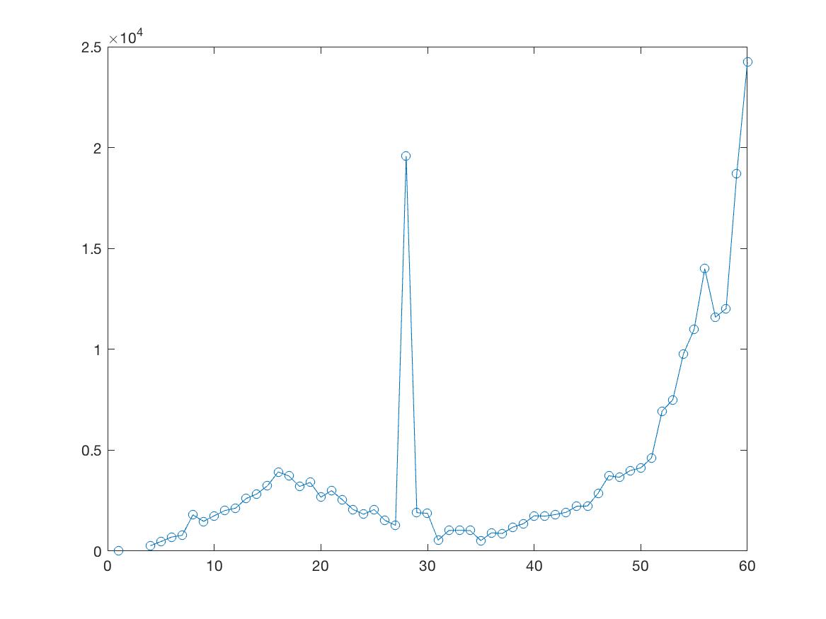
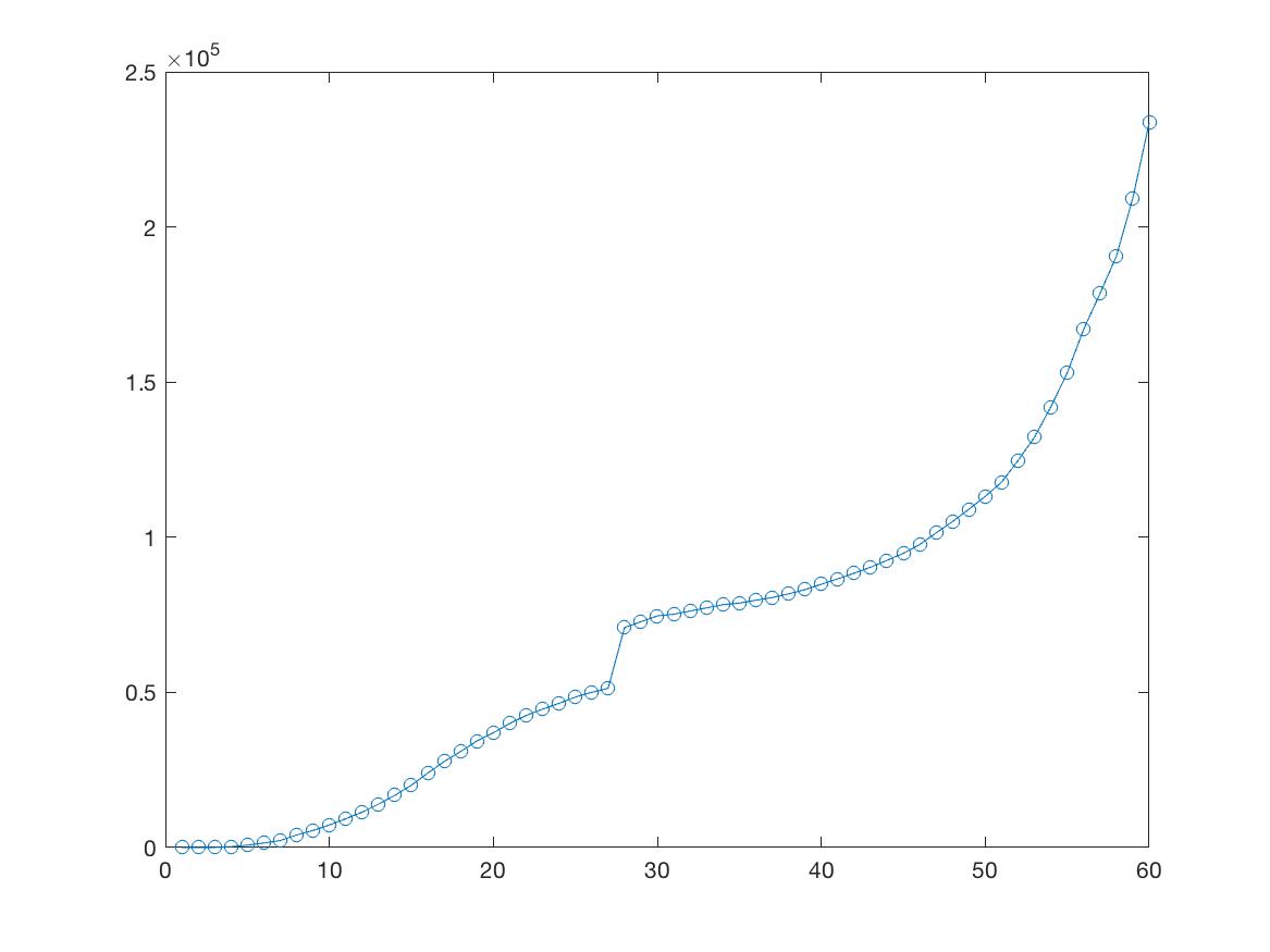
New registered	Total

Figure 1: Raw data for infected globally

The dynamics of the Harris, Lotka-Nagaev and Crump-Hove estimators can be followed on Figure 2.

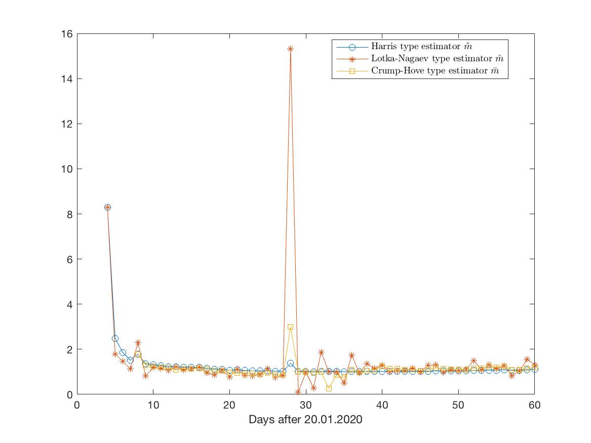
Figure 2: Dynamics of the mean numbers of of the new contaminated individuals

The Harris estimator shows a relatively more stable behaviour during the period. The three estimates exhibit similar asymptotics.

The next step is to calculate the mean values of the expected number of nonregistered contaminated individuals for the three types of estimators, starting with $s=20$ (Figure 3). The last five points on the graph after day 20 represent the forecast for the next 5 days.

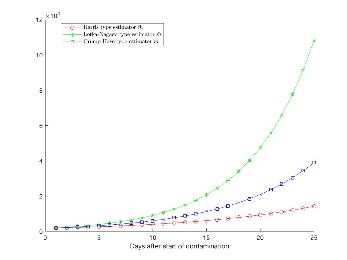
Figure 3: The mean values of the expected number of nonregistered

The corresponding values of the proportion of the registered individuals among the contaminated population is presented on Figure 4

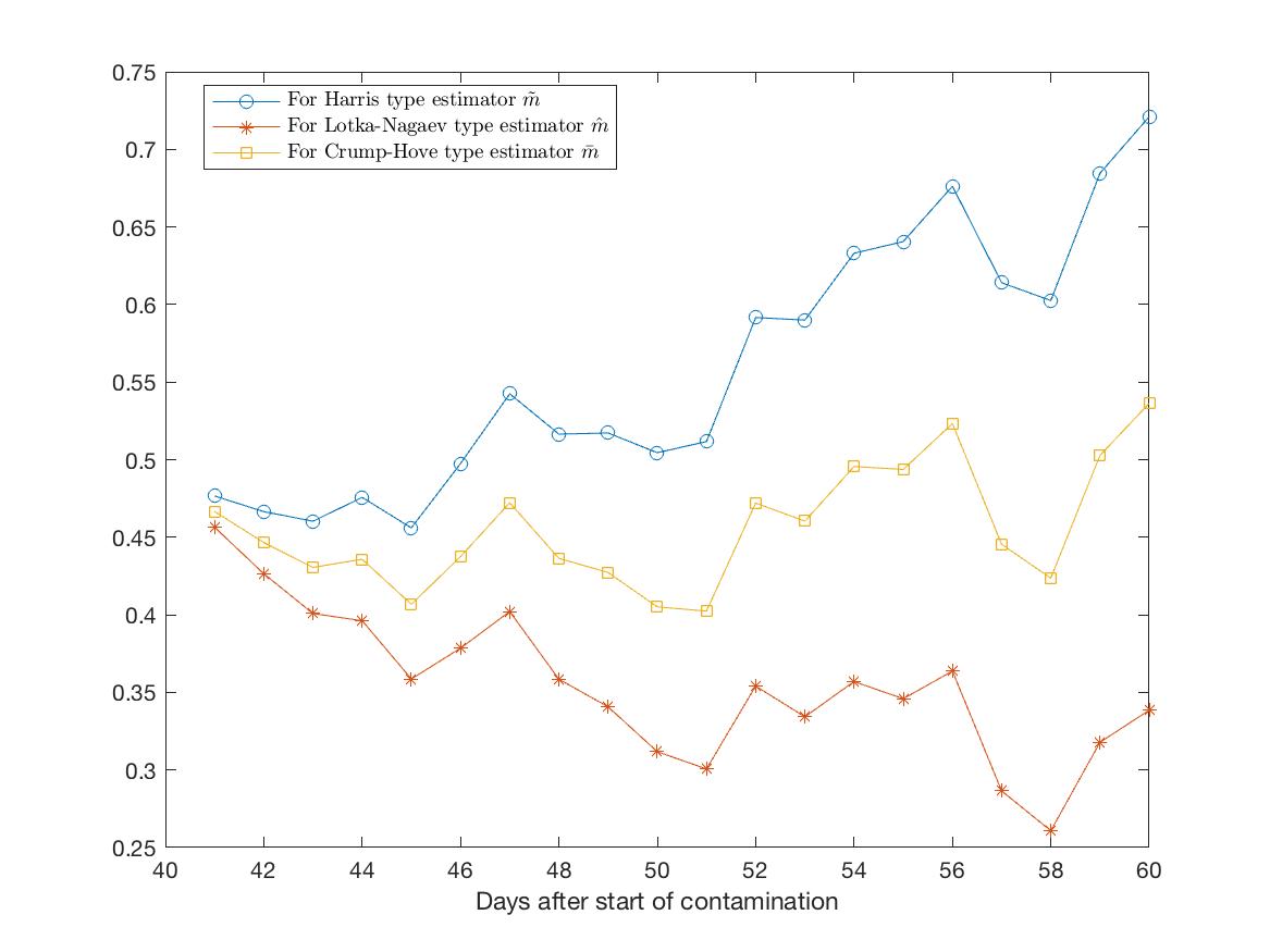
Figure 4: The proportion of the registered individuals

For the registered cases in Italy the raw data can be seen on the Figures 5 - 8 below.

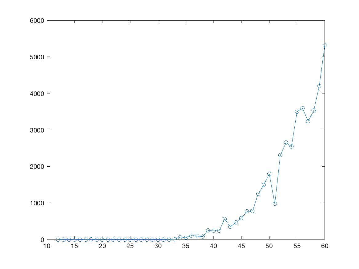
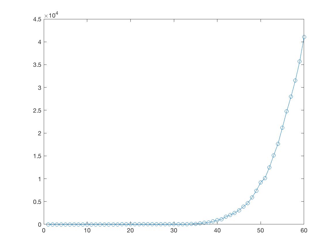
New registered	Total

Figure 5: Raw data, infected, Italy

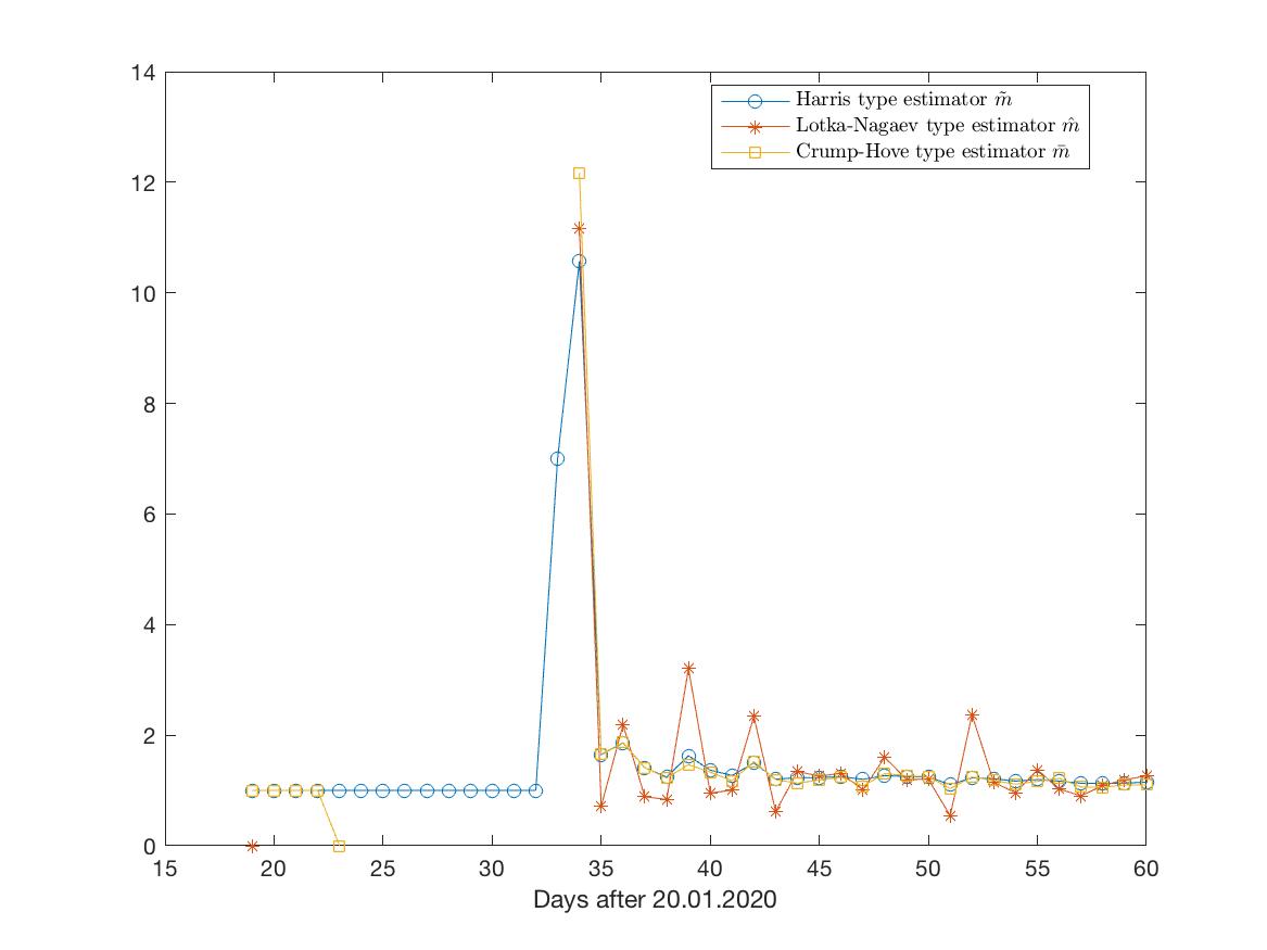
Figure 6: Dynamics of the mean numbers of of the new contaminated individuals

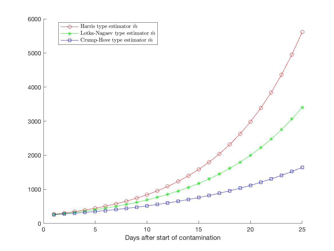
Figure 7: The mean values of the expected number of nonregistered

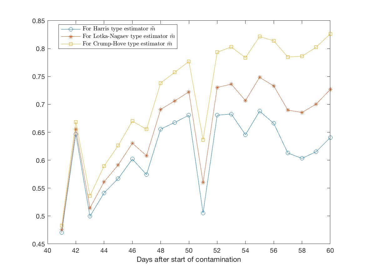
Figure 8: The proportion of the registered individuals

Note that the newly confirmed contaminated individuals in Bulgaria are reported day by day, starting from 08.03.2020 as:
$4;0;2;1;16;8;10;10;11;19;11;18;17;36;22;16;19;22;22;29;38$

In fact these data form the sample $(Z_{2}(1),Z_{2}(2),...,Z_{2}(20)),$ where now $n=20,$ i.e. $20$ days from the first confirmed contaminated individuals. We use also the statistics $U(k)=\sum_{j=1}^{k}Z_{2}(j),k=1,2,...,17,$ whose values are given as follows:
$4;4;6;7;23;31;41;51;62;81;92;110;127;163;185;201;220;242;264;293;331.$

The two samples are presented on Figure 9.

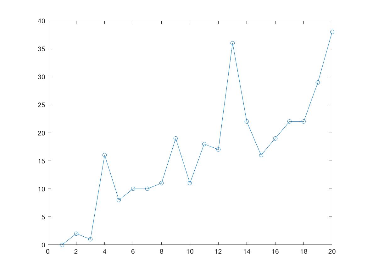
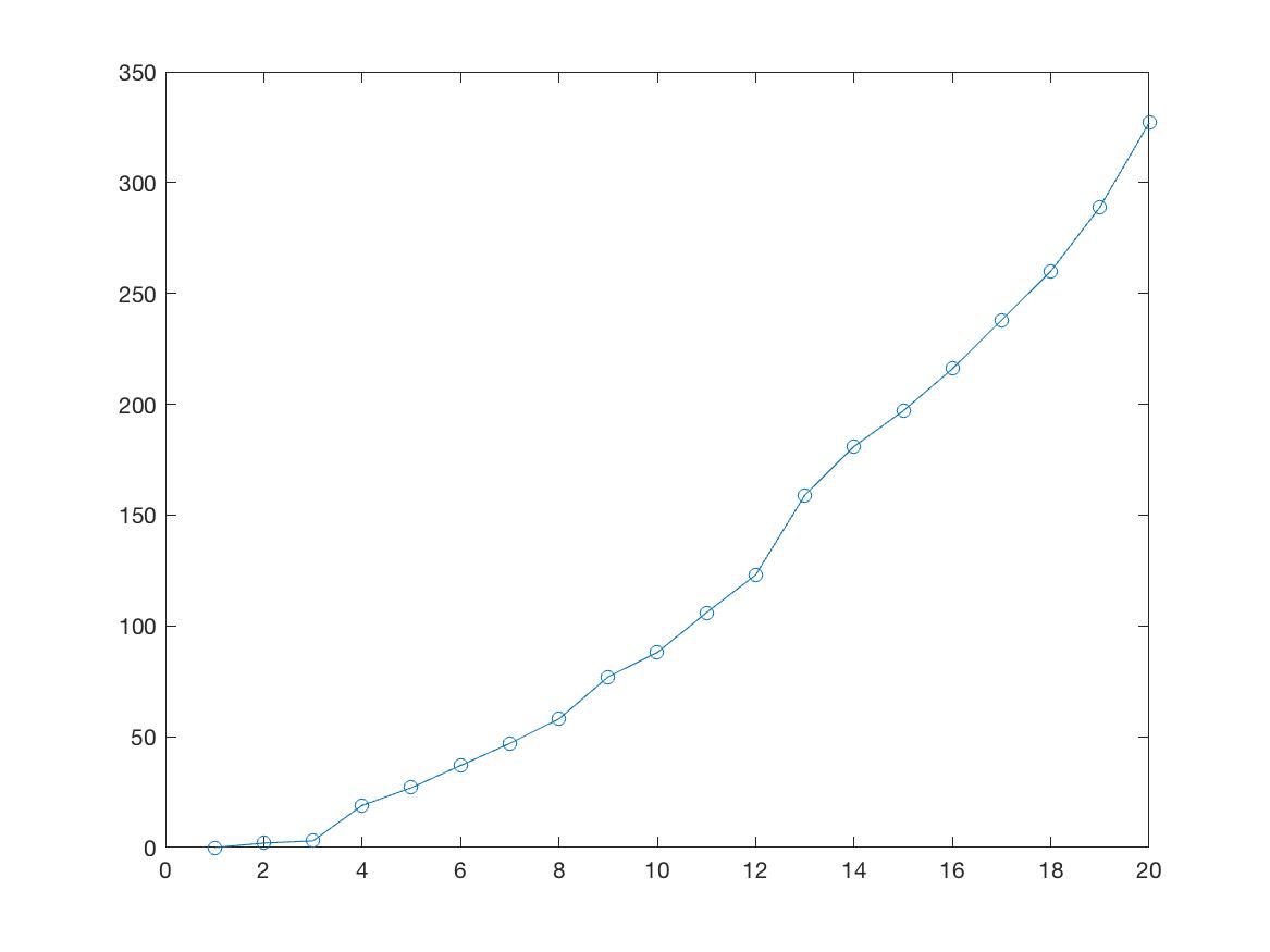
New registered	Total

Figure 9: Raw data, infected, Bulgaria

The estimated mean number of infected individuals for the three types of estimators is presented on Figure 10, the estimated expected number of contaminated individuals (with $s=10$, chosen on the basis of the shorter time period of contamination) can be seen on Figure 11 and the estimated $\alpha$ - on Figure 12.

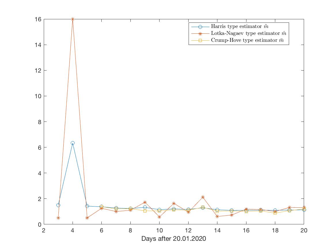
Figure 10: Dynamics of the mean numbers of of the new contaminated individuals

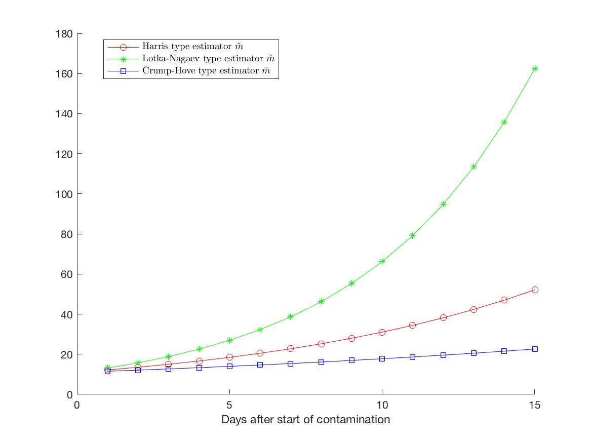
Figure 11: The mean values of the expected number of nonregistered

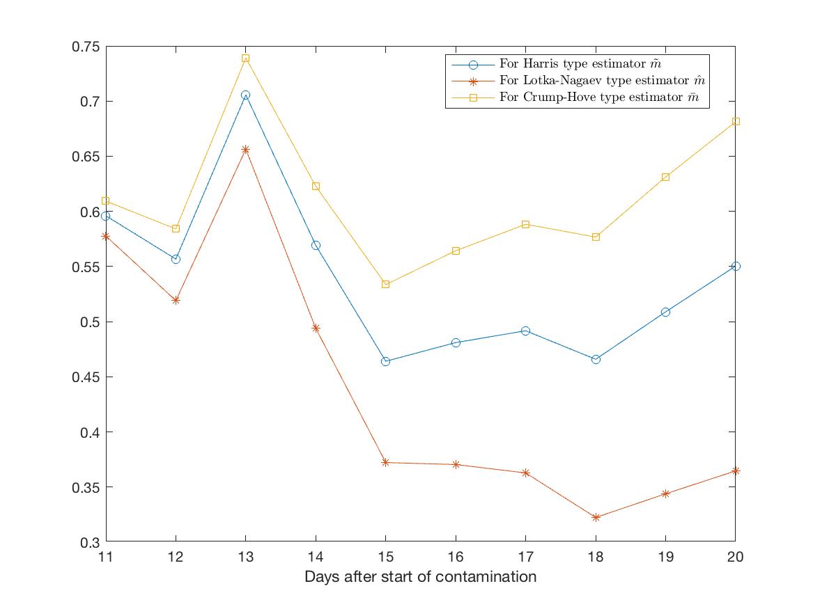
Figure 12: The proportion of the registered individuals

The values of the Harris estimator at the end of the contamination period for the three datasets considered above can be found in Table 1

Data set	$\tilde{m}_{n}$	95% CI lower	95% CI upper
Globally	1.0875	0.9344	1.2406
Italy	1.1348	1.0694	1.2002
Bulgaria	1.1093	0.8845	1.3341

Table 1: Values of the Harris estimator

Up to day 20 the Harris estimator (for Bulgaria) is 1.1093 (i.e. slightly supercritical), the expected number of newly infected and still not registered individuals is appr. 31, the actual reported registered is 38, hence the estimated proportion of the registered individuals among the infected is $\alpha=0.5507$.

To approve the behaviour of the model one can compare the predicted number of confirmed individuals $\tilde{Z}_{2}(n-k)$ (using the Harris estimator $\tilde{m}_{n}$) for the period of $k$ days before the latest date in the data set with the actually observed values of $Z_{2}(n)$. The corresponsing values, as well as the 95% confidence interval of the forecast are presented on Table 2.

Data set	day $k$	$\tilde{Z}_{2}(n-k)$	$Z_{2}(n-k)$	95% CI lower	95% CI upper
Globally	5	11754	13998	8289	15393
	4	15128	11596	10364	19757
	3	12515	12016	8454	16575
	2	12928	18712	8556	17416
	1	20174	24234	12802	27250
Italy	5	4172	3590	3460	4444
	4	4232	3233	3555	4646
	3	3770	3526	3236	4304
	2	4027	4207	3532	4780
	1	4754	5322	4196	5843
Bulgaria	5	19	19	10	25
	4	21	22	11	31
	3	24	22	12	37
	2	24	29	11	38
	1	32	38	15	53

Table 2: Observed and predicted registered cases

Additionaly, using the data, provided by WHO the comparison between the behaviour of the process under different local conditions with a approximatelly same contamination period. For example on the Figure 13 the Harris estimator globally, for Italy, Germany and France are compared.

As mentioned earlier the mean number of new contaminated individuals by one c.i. tends to values close, but greater than 1 as the time of contamination increases.

Calculating the proportions $\alpha$ of the confirmed contaminated individuals among the four populations with $s=20$ (presented on Figure 14) one can see that $\alpha$’s vary largely but stay relatively high, especially at the end of the contamination period. This fact can be considered as a result of different types of actions, undertaken to restrict the spread of the infection.

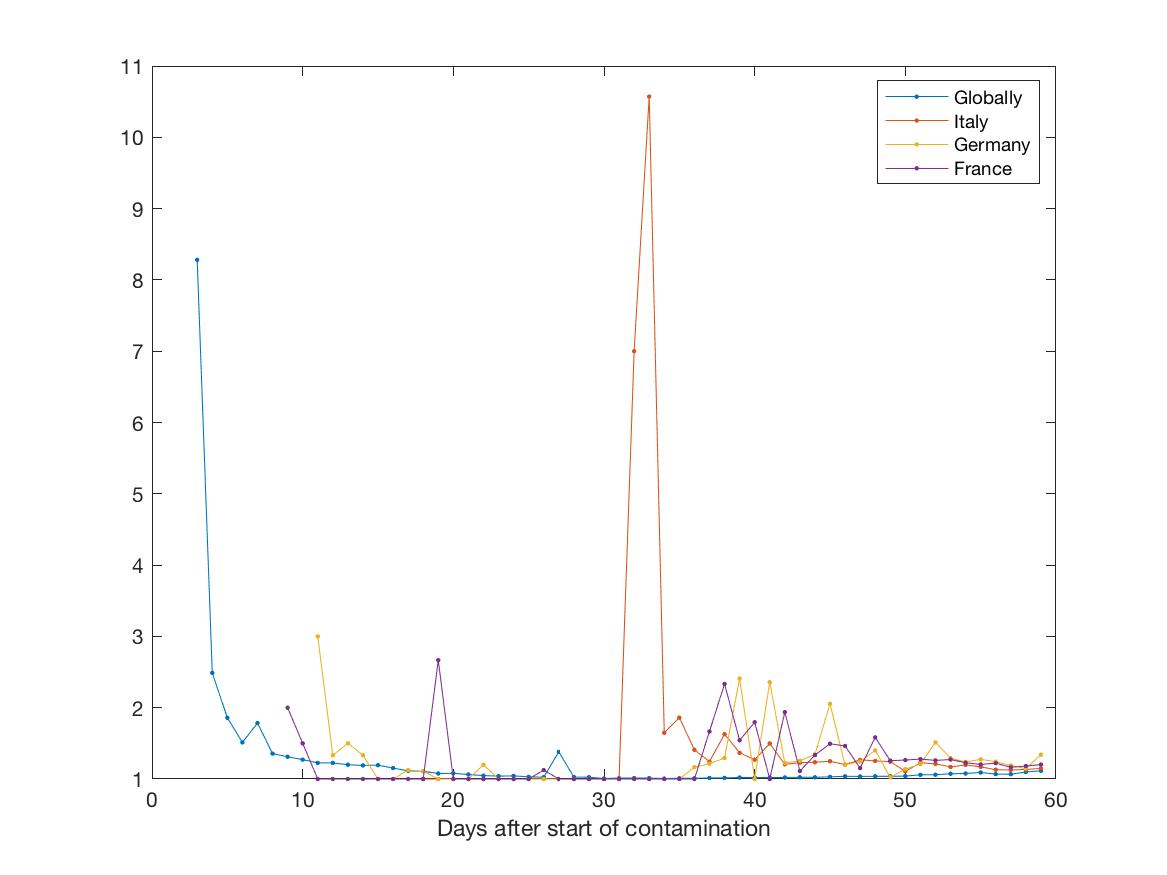
Figure 13: Harris estimator

Figure 14: The proportion of the registered individuals in the last 20 days

4. Concluding remarks.

First of all the estimation of the mean value of reproduction $m$ allows us to classify the contamination process as supercritical ($m>1$), critical ($m=1$) and subcritical ($m<1$). In the supercritical case the mean population growth is exponential, in the critical case the mean value of the population is constant and in the subcritical case the decreasing of the mean population is exponential.

Up to the moment of our investigation the estimated mean number of new contaminated individuals (for Bulgaria) is slightly greater than 1 which corresponds to the exponential growth of the contaminated population, globally and locally in specific countries and regions.

Finally the estimating of the mean parameter of contamination can be considered as a first stage to construction of a more complicated epidemiological model. As a such model for example, one can use a branching process with random migration considered in [8-9] or some other model of controlled branching processes (see [5]).

Additional information, reports and plots, related to this research can be found on http://ir-statistics.net/covid-19.

References

1. Harris, T.E. The Theory of Branching Processes. Springer, Berlin, 1963.

2. Sevastyanov, B.A. Branching Processes. Nauka, Moscow, 1971. (In Russian).

3. Athreya, K.B., P.E. Ney. Branching Processes. Springer, Berlin, 1972.

4. Jagers, P. Branching Processes with Biological Applications. Wiley, London,1975.

5. Gonzalez, M., I.M. del Puerto, G.P. Yanev. Controlled Branching Processes. Wiley, London, 2018.

6. Yakovlev, A. Yu., N. M. Yanev. Transient Processes in Cell Proliferation Kinetics. Lecture Notes in Biomathematics 82, Springer, New York, 1989.

7. Yanev, N.M. Statistical inference for branching processes, Ch.7 (143-168) in: Records and Branching processes, Ed. M.Ahsanullah, G.P.Yanev, Nova Science Publishers, Inc., New York, 2008.

8. Yanev,G.P., N.M. Yanev. Critical branching processes with random migration. In: C.C. Heyde (Editor), Branching Processes (Proceedings of the First World Congress). Lecture Notes in Statistics, 99, Springer-Verlag, New York, 1995, 36-46.

9. Yanev, G.P., N.M. Yanev. Branching Processes with two types of emigration and state-dependent immigration. In: Lecture Notes in Statistics 114, Springer-Verlag, New York, 1996, 216-228.

10. https://www.who.int/emergencies/diseases/novel-coronavirus-2019/situation-reports/ (visited on 20.03.2020)

¹Institute of Mathematics and Informatics, Bulgarian Academy of Sciences

²Faculty of Mathematics and Informatics, Sofia University

³New Bulgarian University