Unambiguous scattering matrix for non-Hermitian systems

Abstract

$\mathcal{PT}$ symmetry is a unique platform for light manipulation and versatile use in unidirectional invisibility, lasing, sensing, etc. Broken and unbroken $\mathcal{PT}$-symmetric states in non-Hermitian open systems are described by scattering matrices. A multilayer structure, as a simplest example of the open system, has no certain definition of the scattering matrix, since the output ports can be permuted. The uncertainty in definition of the exceptional points bordering $\mathcal{PT}$-symmetric and $\mathcal{PT}$-symmetry-broken states poses an important problem, because the exceptional points are indispensable in applications as sensing and mode discrimination. Here we derive the proper scattering matrix from the unambiguous relation between the $\mathcal{PT}$-symmetric Hamiltonian and scattering matrix. We reveal that the exceptional points of the scattering matrix with permuted output ports are not related to the $\mathcal{PT}$ symmetry breaking. Nevertheless, they can be employed for finding a lasing onset as demonstrated in our time-domain calculations and scattering-matrix pole analysis. Our results are important for various applications of the non-Hermitian systems including encircling exceptional points, coherent perfect absorption, $\mathcal{PT}$-symmetric plasmonics, etc.

I Introduction

Scattering is a powerful tool for investigating diverse phenomena in Nature. Due to the interaction of a probe particle (electron, neutron, photon, etc.) with a target, the former changes its characteristics that can be measured by detectors. Independent of the type of the probe particle, the description of such an open system can be performed via the scattering matrix connecting input and output channels Newton .

One of the demanded applications of the scattering matrices is the parity-time ($\mathcal{PT}$)-symmetric systems, implying invariance under simultaneous inversion of the spatial coordinates and time Bender1998 ; Bender2007 . A $\mathcal{PT}$-symmetric system is an example of a non-Hermitian system with the Hamiltonian $\hat{H}\neq\hat{H}^{\dagger}$, where the superscript ${\dagger}$ stands for the Hermitian conjugation. The $\mathcal{PT}$-symmetric non-Hermitian system can have a real-valued spectrum of the operator $\hat{H}=\hat{p}^{2}/2m+\hat{V}$, if the potential meets the condition $V({\rm r})=V^{\ast}(-{\rm r})$.

Being introduced in the framework of quantum mechanics, the $\mathcal{PT}$ symmetry has attracted a lot of attention in photonics recently (see the review articles Zyablovsky2014 ; Feng2017 ; El-Ganainy2018 ; Ozdemir2019 ; Miri2019 ). Using the analogy between the Helmholtz and Schrödinger equations, one can determine optical system’s Hamiltonian with the real-valued spectrum. Dielectric permittivity $\varepsilon$ plays the role of the potential in photonics. That is why the $\mathcal{PT}$ symmetry requires $\varepsilon({\rm r})=\varepsilon^{\ast}(-{\rm r})$ in optics, i.e. loss and gain should be balanced. Remarkably, such systems can be fabricated in different designs: the couple of waveguides Ruter2010 , the two-dimensional array of waveguides Regensburger2012 ; Kremer2019 , the passive multilayer Feng2014 , and the coupled meta-atom systems Lawrence2014 . Along with an anisotropic transmission Ge2012 and unidirectional invisibility Lin2011 ; Feng2013 , intriguing physics arises in the vicinity of exceptional points, where a phase transition between $\mathcal{PT}$- and non-$\mathcal{PT}$-symmetric phases occurs Ozdemir2019 ; Miri2019 . The exceptional points can be used as a platform for an optical omnipolarizer Hassan2017 and sensor with unprecedented sensibility Chen2017 ; Hodaei2017 . In the $\mathcal{PT}$-symmetry-broken state, a system has exponentially decaying and amplifying modes, thus giving an opportunity for lasing Feng2014-2 ; Hodaei2014 ; Gu2016 and coherent perfect absorption Longhi2010 ; Chong2011 ; Wong2016 .

Scattering matrix can be written in terms of the Hamiltonian $\hat{H}$ as $\hat{S}=\exp\left(-i\hat{H}(t-t_{0})/\hbar\right)$, where $\hbar$ is the reduced Planck constant. It relates the input wave at the moment $t_{0}$ with the output wave at the moment $t$. For the real-valued spectrum $\lambda_{n}$ of the $\mathcal{PT}$-symmetric Hamiltonian, we naturally obtain the unimodular eigenvalues $s_{n}=\exp(-i\lambda_{n}(t-t_{0})/\hbar)$ of the scattering matrix: $|s_{n}|=1$. Thus, the eigenvalues $s_{n}$ usually fully define, whether the state of a system is $\mathcal{PT}$-symmetric or not. However, this may not be the case, if the scattering matrix is introduced irrespective of the Hamiltonian. Then the input and output channels can be permuted resulting in the scattering matrices with different eigenvalues. Uncertainty in the definition of the scattering matrix is inadmissible and can mislead during interpretation of results. Such situation arises for one-dimensional (1D) multilayer structures shown in Fig. 1. In this paper, we analyze the definitions of the scattering matrix widely used in $\mathcal{PT}$-symmetry studies, discuss their physical meaning and successfully solve the problem of unique choice of the scattering matrix.

II Problem of the scattering matrix uniqueness

Scattering matrix of a 1D $\mathcal{PT}$-symmetric multilayer system schematically shown in Fig. 1 is usually defined as

$$\hat{S}_{1}=\left(\begin{array}[]{cc}r_{L}&t\\ t&r_{R}\end{array}\right)\quad{\rm or}\quad\hat{S}_{2}=\left(\begin{array}[]{cc}t&r_{R}\\ r_{L}&t\end{array}\right),$$ (1)

where $t$, $r_{L}$, and $r_{R}$ are the complex transmission, reflection-to-the-left, and reflection-to-the-right coefficients, respectively. The definitions differ in how we write the vector of output fields: either $(b_{L},b_{R})^{T}=\hat{S}_{1}(a_{L},a_{R})^{T}$ or $(b_{R},b_{L})^{T}=\hat{S}_{2}(a_{L},a_{R})^{T}$, where the superscript $T$ means the transposition, $a_{L,R}$ and $b_{L,R}$ are the input and output fields, respectively (see Fig. 1). It seems quite not important, which matrix should be used, because they result in the same output fields. However, this difference appears dramatically important, when we are looking for the exceptional points bordering the $\mathcal{PT}$-symmetric and $\mathcal{PT}$-symmetry-broken states. Indeed, the eigenvalues $s_{1,2}$ of the scattering matrix should be unimodular ($|s_{1,2}|=1$) in the $\mathcal{PT}$-symmetric state and inverse ($|s_{1}|=1/|s_{2}|$) in the $\mathcal{PT}$-symmetry-broken phase. The two definitions Eq. (1) of the scattering matrix provide different eigenvalues $s_{1,2}^{(1)}=(r_{R}+r_{R})/2\pm\sqrt{t^{2}+(r_{L}-r_{R})^{2}/4}$ and $s_{1,2}^{(2)}=t\pm\sqrt{r_{L}r_{R}}$ for $\hat{S}_{1}$ and $\hat{S}_{2}$, respectively. Therefore, the violation of $\mathcal{PT}$ symmetry appears under different conditions. This situation is confusing and unacceptable.

The scattering matrix $\hat{S}_{2}$ is used in most articles on $\mathcal{PT}$ symmetry. Diverse phenomena have been described with its help including unidirectional invisibility Lin2011 , optical pulling Alaee2018 , and photonic spin Hall effect Zhou2019 . Ambiguity of the definition of the scattering matrix was discussed in several works Ge2012 ; Mostafazadeh . In particular, L. Ge et al. in Ref. Ge2012 advocate for $\hat{S}_{1}$ justifying this by the decisive comparison. In particular, the exceptional points obtained using the scattering matrix $\hat{S}_{1}$ are in good correspondence to the lasing onset associated to breaking the loss-gain balance in $\mathcal{PT}$-symmetric structures Ge2012 . This feature was used to predict the properties of the systems acting simultaneously as a laser and coherent perfect absorber Achilleos2017 ; Chong2011 ; Novitsky2019 , as well as to study the lasinglike nonstationary behavior above the $\hat{S}_{1}$ exceptional point Novitsky2018 . Nevertheless, the matrix $\hat{S}_{1}$ is rarely exploited in comparison to $\hat{S}_{2}$.

III Balance of the loss and gain

$\mathcal{PT}$-symmetric phase is characterized by the balance of loss and gain. Therefore, first, we try to solve the dilemma “$\hat{S}_{1}$ vs. $\hat{S}_{2}$” using the assumption that only a proper scattering matrix guarantees such a balance. The balance can be quantified as a zero difference between the energies concentrated in the loss and gain layers: $\Delta w=\left|\int_{0}^{d}|{\bf E}_{L}|^{2}dz-\int_{d}^{2d}|{\bf E}_{G}|^{2}dz\right|$. The energy balance is a property of the system and, therefore, can be calculated irrespective of the scattering matrix. To this end, we specify one of the input amplitudes $a_{L}=|a_{L}|$ and find the complex value $a_{R}$ to reach the balance. Since $a_{R}$ is characterized by the absolute value $|a_{R}|$ and the argument $\phi$ (in fact, the phase difference with $a_{L}$), we plot condition of the balance (at given $\varepsilon^{\prime\prime}$) as curves in the coordinates $(|a_{R}/a_{L}|,\phi)$ in Fig. 2(a). For a scattering matrix, the amplitudes take certain values being its eigenvector $(a_{L},a_{R})^{T}$. These amplitudes correspond to a point on the curve of the energy balance. In fact, for the scattering matrix $\hat{S}_{1}$ the energy balance is achieved at $|a_{R}|=|a_{L}|$, i.e. right and left input fields differ only in phase [point 2 in Fig. 2(a)]. The loss and gain for the scattering matrix $\hat{S}_{2}$ are balanced, when the left and right input fields are in phase, $\phi=0$, and have different magnitudes $|a_{R}|\neq|a_{L}|$ [point 1 in Fig. 2(a)]. We emphasize, however, that the balance of loss and gain appears not only at the points 1 and 2, but occupy a curve. Each point on the curve have a symmetric energy distribution as demonstrated in Fig. 2(b) for points 1, 2, and 3 (the latter is calculated at $\varepsilon^{\prime\prime}=5$). Point 4 is displaced from the proper curve and, therefore, a non-symmetric field distribution is seen in this case. Since the scattering matrices are related as $\hat{S}_{2}=\left(\begin{array}[]{cc}0&1\\ 1&0\end{array}\right)\hat{S}_{1}$, we can assume that the loss and gain balance in point 3 might correspond to another scattering matrix $\hat{S}_{3}=B\hat{S}_{1}$, where $B$ is an auxiliary matrix. Then there are infinitely many scattering matrices that can be obtained from $\hat{S}_{1}$ using the multiplication by this auxiliary matrix. So, the study of balance conditions cannot solve the problem of the proper scattering matrix.

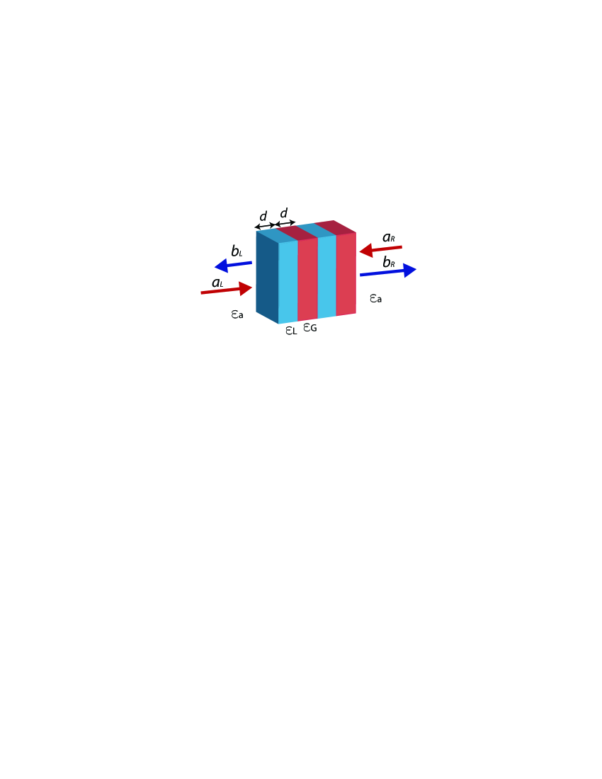
Figure 1: $\mathcal{PT}$-symmetric multilayer system with alternating loss and gain slabs. We employ parameters $d=50$ nm and $\varepsilon_{a}=1$ through the paper.

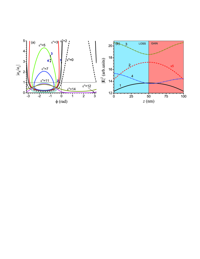
Figure 2: (a) Curves of the loss and gain balance (difference of the energy in loss and gain layers) for different $\varepsilon^{\prime\prime}$ in a bilayer. (b) Energy density across the bilayer for points 1 to 4 in (a). $|a_{R}|$ and $\phi$ are the absolute value and argument of the complex amplitude $a_{R}$ at fixed $a_{L}=1$ The real part of permittivity is $\varepsilon^{\prime}=2$.

IV Derivation of the scattering matrix

In quantum mechanics, a system is $\mathcal{PT}$-symmetric, if its Hamiltonian $\hat{H}$ commutes with the parity $\hat{P}$ and time $\hat{T}$ operators. Such a non-Hermitian Hamiltonian can possess real eigenvalues $\lambda$, which can be found from the stationary Schrödinger equation, $\hat{H}\phi=\lambda\phi$. Time evolution of such a system follows from the temporal Schrödinger equation $i\hbar\partial\psi/\partial t=\hat{H}\psi$. If $\hat{H}$ is time independent, one arrives at

$$\psi({\bf r},t)=\exp\left(-\frac{i\hat{H}t}{\hbar}\right)\psi({\bf r},0).$$ (2)

This solution means that the initial state $\psi({\bf r},0)$ is transformed into $\psi({\bf r},t)$ after some time $t$. The operator connecting the wave functions before and after scattering is a scattering matrix $\hat{S}=\exp\left(-i\hat{H}t/\hbar\right)$. Commutation $[\hat{S},\hat{H}]=0$ results in the same set of the eigenfunctions for these operators: $\hat{S}\phi=\mu\phi$, where $\mu=\exp(-i\lambda t/\hbar)$. For a system in the $\mathcal{PT}$-symmetric state, $\lambda$ is real-valued, hence, $\mu$ is unimodular, $|\mu|=1$. It is important that the scattering operator is unambiguously determined by the Hamiltonian. We aim to find the scattering matrix for multilayer systems in a similar manner.

Let us consider 1D propagation of a plane electromagnetic wave through a $\mathcal{PT}$-symmetric multilayer system with dielectric permittivity $\varepsilon(z)=\varepsilon^{\ast}(-z)$. The 1D propagation implies dependence of the electric ${\bf E}(z,t)$ and magnetic ${\bf H}(z,t)$ fields on the single spatial coordinate $z$ in the direction of the unit vector ${\bf q}$ normal to the slabs. Then the Maxwell equations can be formally written in the form of the temporal Schrödinger equation

$$i\hbar\frac{\partial}{\partial t}\left(\begin{array}[]{c}{\bf H}(z,t)\\ {\bf E}(z,t)\end{array}\right)=\hat{H}\left(\begin{array}[]{c}{\bf H}(z,t)\\ {\bf E}(z,t)\end{array}\right),$$ (3)

where the Hamiltonian is equal to

$$\hat{H}=i\hbar c{\bf q}\times\left(\begin{array}[]{cc}0&-1\\ \varepsilon^{-1}(z)&0\end{array}\right)\frac{\partial}{\partial z}.$$ (4)

For the $\mathcal{PT}$-symmetric multilayer, the Hamiltonian is invariant under the simultaneous space and time inversion. The scattering matrix $\hat{S}=\exp\left(-i\hat{H}t/\hbar\right)$ connects the fields before and after scattering as

$$\left(\begin{array}[]{c}{\bf H}(t)\\ {\bf E}(t)\end{array}\right)=\hat{S}\left(\begin{array}[]{c}{\bf H}(0)\\ {\bf E}(0)\end{array}\right).$$ (5)

Without loss of generality further we assume a specific polarization. The fields before scattering are the input fields $H_{y}(0)=H_{y}^{LR}(0)+H_{y}^{RL}(0)$ and $E_{x}(0)=E_{x}^{LR}(0)+E_{x}^{RL}(0)$: from the left to right $H_{y}^{LR}(0)$, $E_{x}^{LR}(0)=\gamma_{a}H_{y}^{LR}(0)$ and from the right to left $H_{y}^{RL}(0)$, $E_{x}^{RL}(0)=-\gamma_{a}H_{y}^{RL}(0)$, where $\gamma_{a}=1/\sqrt{\varepsilon_{a}}$ is the surface impedance. Similarly, the output fields $H_{y}(t)=H_{y}^{LR}(t)+H_{y}^{RL}(t)$ and $E_{x}(t)=E_{x}^{LR}(t)+E_{x}^{RL}(t)$ after the scattering read $H_{y}^{LR}(t)$, $E_{x}^{LR}(t)=\gamma_{a}H_{y}^{LR}(t)$ and $H_{y}^{RL}(t)$, $E_{x}^{RL}(t)=-\gamma_{a}H_{y}^{RL}(t)$.

Introducing $a_{L}=H_{y}^{LR}(0)$, $a_{R}=H_{y}^{RL}(0)$, $b_{L}=H_{y}^{RL}(t)$, and $b_{R}=H_{y}^{LR}(t)$, we get

$$\left(\begin{array}[]{c}b_{R}+b_{L}\\ \gamma_{a}(b_{R}-b_{L})\end{array}\right)=\hat{S}\left(\begin{array}[]{c}a_{L}+a_{R}\\ \gamma_{a}(a_{L}-a_{R})\end{array}\right).$$ (6)

The scattering matrix can be written in terms of the reflection $r_{L}$, $r_{R}$ and transmission $t$ coefficients. By substituting the output fields $b_{L}=r_{L}a_{L}+ta_{R}$ and $b_{R}=r_{R}a_{R}+ta_{L}$ into Eq. (6), we have

$$\hat{S}=\left(\begin{array}[]{cc}t+(r_{R}+r_{L})/2&-\gamma_{a}^{-1}(r_{R}-r_{L})/2\\ \gamma_{a}(r_{R}-r_{L})/2&t-(r_{R}+r_{L})/2\end{array}\right).$$ (7)

This scattering matrix is unambiguously connected to the $\mathcal{PT}$-symmetric Hamiltonian and, therefore, correctly describes exceptional points and $\mathcal{PT}$-symmetry violation. The matrix (7) can be presented as $\hat{S}=A\hat{S}_{2}A^{-1}$, where $A=-\frac{1}{2\gamma_{a}}\left(\begin{array}[]{cc}1&1\\ \gamma_{a}&-\gamma_{a}\end{array}\right)$ is the orthogonal rotation matrix. That is why the eigenvalues of the scattering matrices $\hat{S}$ and $\hat{S}_{2}$ coincide. Thus, the matrix $\hat{S}_{2}$ can be used for correct prediction of the exceptional points, where the $\mathcal{PT}$ symmetry gets broken.

The derivation of the scattering matrix (7) discussed above can be supported by additional arguments. If the field is incident from the left, the input field is characterized solely by the amplitude $a_{L}$, while the output fields equal $b_{L}=r_{L}a_{L}$ and $b_{R}=ta_{L}$. Plugging them into Eq. (5) yields

$$\hat{S}\left(\begin{array}[]{c}1\\ \gamma_{a}\end{array}\right)=\left(\begin{array}[]{c}t+r_{L}\\ \gamma_{a}(t-r_{L})\end{array}\right).$$ (8)

When the field comes in from the right-hand side, we have the analogous equation, where $r_{L}$ and $\gamma_{a}$ are replaced with $r_{R}$ and $-\gamma_{a}$, respectively:

$$\hat{S}\left(\begin{array}[]{c}1\\ -\gamma_{a}\end{array}\right)=\left(\begin{array}[]{c}t+r_{R}\\ -\gamma_{a}(t-r_{R})\end{array}\right).$$ (9)

Eqs. (8) and (9) represent 4 equations for 4 unknown elements of the scattering matrix. Solution of these equations gives the same Eq. (7).

V Physical meaning of the exceptional points

V.1 General remarks

Using the generalized unitarity relation $r_{L}r_{R}=t^{2}(1-|t|^{-2})$, the eigenvalues of the scattering matrices can be represented as $s_{1,2}=q(1\pm\sqrt{1-|q|^{-2}})$, where $q=(r_{L}+r_{R})/2$ for $\hat{S}_{1}$ and $q=t$ for $\hat{S}_{2}$ and $\hat{S}$. Then the $\mathcal{PT}$-symmetric state corresponds to $|q|^{2}<1$ resulting in $|s_{1,2}|=1$. For $|q|^{2}>1$, we arrive at the $\mathcal{PT}$-symmetry-broken state with $|s_{1}|=1/|s_{2}|$.

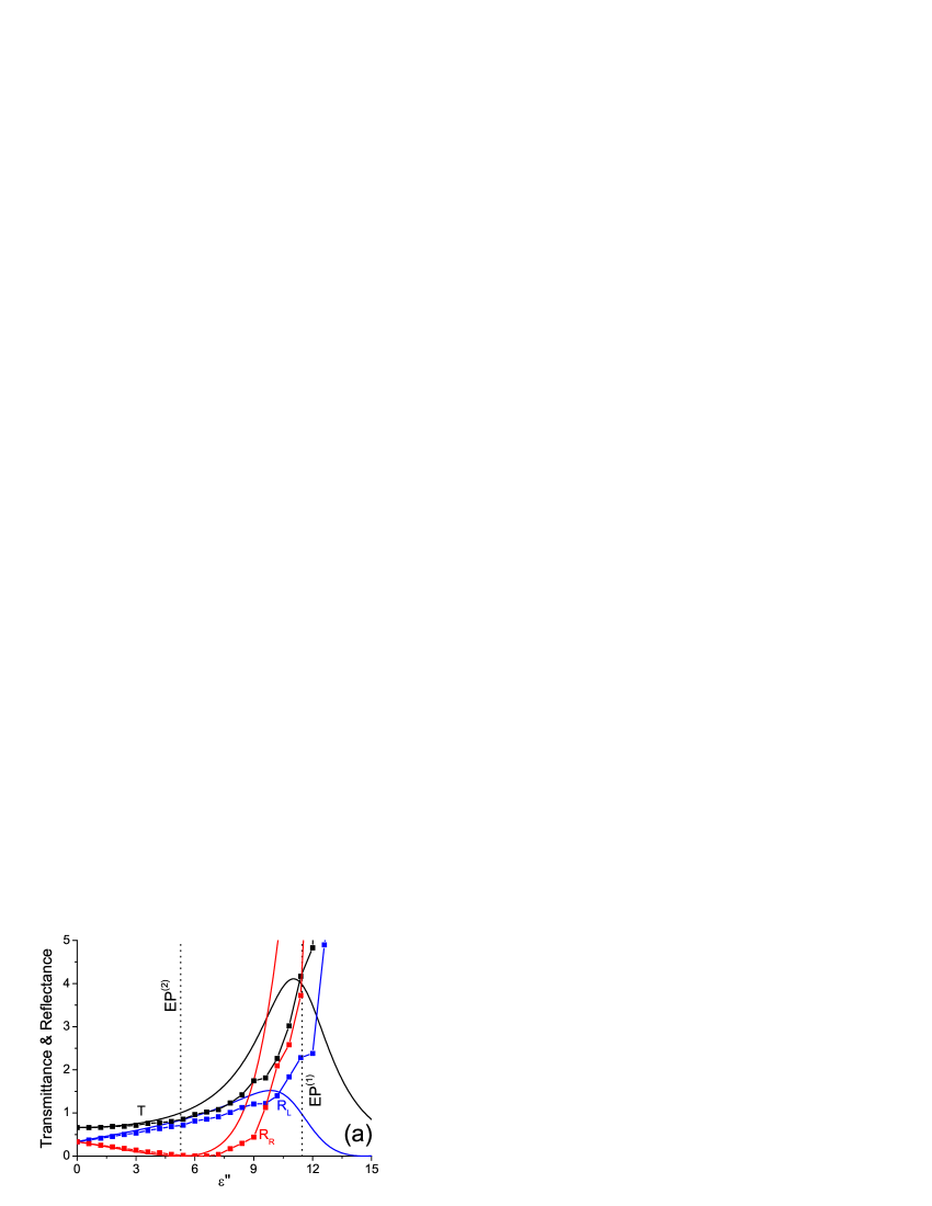
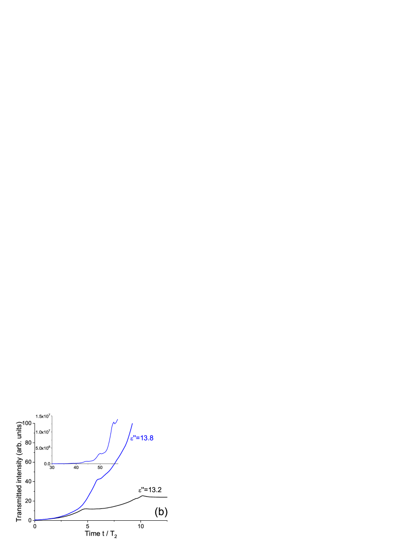
Figure 3: (a) Transmittance $T$ and reflectances $R_{L}$ and $R_{R}$ of the loss-gain bilayer with $\varepsilon^{\prime}=4$ and $d=50$ nm as a function of $\varepsilon^{\prime\prime}$. The results of calculation using the transfer-matrix method and Maxwell-Bloch equations are shown by the solid lines and symbols, respectively. Vertical dotted lines mark positions of the exceptional points calculated using the scattering matrices $\hat{S}_{1}$ (EP⁽¹⁾) and $\hat{S}_{2}$ (EP⁽²⁾). (b) Temporal profiles of transmitted intensity for $\varepsilon^{\prime\prime}$ just below and above the lasing threshold near the EP⁽¹⁾. The inset shows the curve for $\varepsilon^{\prime\prime}=13.8$ on the longer scale.

$\mathcal{PT}$-symmetric phase for $\hat{S}_{2}$ corresponds to $|t|^{2}<1$, while exceptional points follow from $|t|=1$. The exceptional points of the matrix $\hat{S}_{1}$ are defined by the condition $|r_{L}+r_{R}|=2$. Remarkably, it can be met for the great values of reflectances $|r_{L}|^{2}$ and $|r_{R}|^{2}$, if the difference of arguments $|{\rm Arg}(r_{L})-{\rm Arg}(r_{R})|$ is around $\pi$. So, the $\mathcal{PT}$ symmetry breaking via $\hat{S}_{1}$ may occur near poles of the reflection and transmission coefficients and can be used as a predictor of lasing as discussed in Refs. Ge2012 ; Chong2011 ; Novitsky2018 .

V.2 Time-domain simulations

Further we shed light on the role of the exceptional points of $\hat{S}_{1}$ using time-domain calculations of the wave propagation through the bilayer with parameters $\varepsilon^{\prime}=4$ and $d=50$ nm. Treating the loss and gain materials as two-level media, we numerically solve the Maxwell-Bloch equations Novitsky2011 for the complex amplitude of microscopic (atomic) polarization $\rho$, difference between populations of the ground and excited states $w$, and electric field amplitude $A$:

$$\frac{d\rho}{d\tau} = il\Omega w+i\rho\delta-\gamma_{2}\rho,$$ (10)

$$\frac{dw}{d\tau} = 2i(l^{*}\Omega^{*}\rho-\rho^{*}l\Omega)-\gamma_{1}(w-w_{eq}),$$ (11)

$$\frac{\partial^{2}\Omega}{\partial\xi^{2}} - n_{d}^{2}\frac{\partial^{2}\Omega}{\partial\tau^{2}}+2i\frac{\partial\Omega}{\partial\xi}+2in_{d}^{2}\frac{\partial\Omega}{\partial\tau}+(n_{d}^{2}-1)\Omega$$ (12)

$$=3\alpha l\left(\frac{\partial^{2}\rho}{\partial\tau^{2}}-2i\frac{\partial\rho}{\partial\tau}-\rho\right),$$

where $\tau=\omega t$ and $\xi=kz$ are respectively the dimensionless time and distance, $\Omega=(\mu/\hbar\omega)A$ is the normalized Rabi frequency, $\omega$ is the light circular frequency, $k=\omega/c$ is the wavenumber in vacuum, $c$ is the speed of light, $\hbar$ is the reduced Planck constant, and $\mu$ is the dipole moment of the quantum transition. Dimensionless parameter $\alpha=\omega_{L}/\omega=4\pi\mu^{2}C/3\hbar\omega$ is the light-matter coupling strength, where $\omega_{L}$ is the Lorentz frequency and $C$ is the concentration of two-level atoms. $\delta=(\omega_{0}-\omega)/\omega$ is the detuning of the light frequency $\omega$ from the frequency $\omega_{0}$ of the atomic resonance. Normalized relaxation rates of population $\gamma_{1}=1/(\omega T_{1})$ and polarization $\gamma_{2}=1/(\omega T_{2})$ are expressed by means of the longitudinal $T_{1}$ and transverse $T_{2}$ relaxation times. Influence of the polarization of the background dielectric having real-valued refractive index $n_{d}=\sqrt{\varepsilon^{\prime}}$ on the embedded active particles is taken into account by the local-field enhancement factor $l=(n_{d}^{2}+2)/3$ Crenshaw2008 ; Bloembergen .

Equilibrium population difference $w_{eq}$ plays the role of a pumping parameter: it changes from $w_{eq}=1$ (no pump, purely lossy medium) via $w_{eq}=0$ (no loss or gain, saturated medium) to $w_{eq}=-1$ (maximal pump, fully inverted medium). In the steady-state approximation, when a saturation can be neglected ($\Omega\ll\Omega_{sat}=\sqrt{\gamma_{1}(\gamma_{2}^{2}+\delta^{2})/4l^{2}\gamma_{2}}$), one can obtain the expression for the effective permittivity of the two-level medium at the exact resonance $\delta=0$ Novitsky2017 : $\varepsilon_{eff}=\varepsilon^{\prime}+i\varepsilon^{\prime\prime}\approx n_{d}^{2}+3il^{2}\omega_{L}T_{2}w_{eq}$. We assume that the $\mathcal{PT}$-symmetric bilayer is composed of a lossy ($\varepsilon_{eff+}$) and gain ($\varepsilon_{eff-}$) layers, where Novitsky2018

$$\varepsilon_{eff\pm}\approx n_{d}^{2}\pm 3il^{2}\omega_{L}T_{2}|w_{eq}|.$$ (13)

The system is obviously $\mathcal{PT}$-symmetric, because the necessary condition $\varepsilon(z)=\varepsilon^{\ast}(-z)$ is satisfied.

Equations (10)–(12) are solved numerically using the finite-difference approach developed in Ref. Novitsky2009 . An initial value of the population difference is $w(t=0)=w_{eq}$. In our calculations, we assume $\delta=0$ (exact resonance), $n_{d}=2$, $\omega_{L}=10^{11}$ rad$\cdot$s^-1, $T_{1}=1$ ns, and $T_{2}=50$ ps. These parameters correspond to the semiconductor quantum dots as the active particles Palik ; Diels . The loss and gain layers have the same thickness $d=50$ nm. The incident monochromatic light has the wavelength $\lambda=1$ $\mu$m and the intensity much lower than the saturation intensity. These parameters might correspond, e.g., to the quantum dots as two-level atoms, but the other systems with properly chosen parameters can be also considered. The side-pumping scheme similar to that realized by Wong et al Wong2016 can be employed for excitation of the materials.

In Fig. 3(a), we compare the transmittance and reflectance calculated using the time-domain (TD) and transfer-matrix (TM) techniques. The positions of the exceptional points EP⁽¹⁾ and EP⁽²⁾ for the corresponding scattering matrices $\hat{S}_{1}$ and $\hat{S}_{2}$ divide the whole space of $\varepsilon^{\prime\prime}$ into three regions. There is a good agreement between the TD and TM methods at low $\varepsilon^{\prime\prime}$ (first region), including the position of EP⁽²⁾ corresponding to the condition of a unidirectional reflectionlessness Ge2012 . Between the exceptional points EP⁽¹⁾ and EP⁽²⁾ (second region), there is a divergence between the results given by the TD and TM methods, in accordance with the previous observations Novitsky2018 . Both reflectances and transmittance are larger for the TM approach. There are several reasons for this discrepancy. First, the linearized expression for permittivity (13) used in TM calculations gives less correct results for larger gain and loss, since it does not take into account the nonlinear effect of saturation. As a result, the TM method neglecting nonlinearity gives somewhat overestimated transmission and reflection in comparison to the TD simulations. Second, the spatial discretization used in the TD simulations can influence the calculations for large gain, since the amplification of radiation per every spatial step becomes more significant. Nevertheless, the general trends of transmission and reflection change are consistent for both calculation methods.

Above the EP⁽¹⁾ (third region), the situation dramatically changes, because the system loses stability and goes into the lasinglike mode described within the TD technique. The development of lasing can be more vividly observed in the temporal dynamics illustrated in Fig. 3(b): a comparatively small increase in $\varepsilon^{\prime\prime}$ results in the transfer from the regime of a stationary state establishment to exponentially increasing intensity. Limited by the saturation, the exponential increase results in the formation of a powerful pulse as analyzed in Ref. Novitsky2018 . Here we show only proof-of-concept results and the values of $\varepsilon^{\prime\prime}$ necessary for observing these effects can be made much lower for the greater number of layers and thicker slabs.

Thus, from the dynamical considerations, we deduce three regimes of the light interaction: (i) the $\mathcal{PT}$-symmetric state with balanced loss and gain below the EP⁽²⁾, (ii) the $\mathcal{PT}$-symmetry-broken state with imbalanced loss and gain, but nevertheless stationary levels of reflection and transmission (between EP⁽¹⁾ and EP⁽²⁾), and (iii) the $\mathcal{PT}$-symmetry-broken state with nonstationary (lasinglike) mode of radiation above EP⁽¹⁾. Wave propagation in a $\mathcal{PT}$-symmetric system emulates propagation in lossless medium with $T<1$, when the loss and gain compensate each other. This qualitatively explains that $T>1$ requires violation of the $\mathcal{PT}$ symmetry in agreement with the $\hat{S}_{2}$ behavior. To the contrast, lasing phenomenon is not connected with the $\mathcal{PT}$ symmetry breaking. This latter regime needs to be discussed in more detail.

V.3 Lasing onset and pole analysis

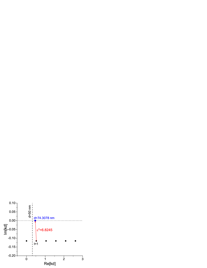
Figure 4: The positions of the poles in the complex-frequency plane. The cases of the lossless bilayer (black dots) and the bilayer with $\varepsilon^{\prime\prime}=6.8245$ (blue dot) are shown.

Lasing is usually associated with poles of the scattering matrix arising at the real frequencies, where both reflection and transmission coefficients tend to infinity. In the case of a bilayer with refractive indices $n_{L}=\sqrt{\varepsilon_{L}}$ and $n_{G}=\sqrt{\varepsilon_{G}}$, positions of the poles in the complex frequency plane can be found semianalytically from equation

$$\left(\frac{n_{L}}{n_{G}}+\frac{n_{G}}{n_{L}}\right)\tan{kdn_{L}}\tan{kdn_{G}}$$ (14)

$$+ i\left[\left(n_{L}+\frac{1}{n_{L}}\right)\tan{kdn_{L}}+\left(n_{G}+\frac{1}{n_{G}}\right)\tan{kdn_{G}}\right]$$

$$- 2=0,$$

where $kd=2\pi d/\lambda$ is the normalized frequency. Solving Eq. (14), one obtains the positions of the poles on the complex-frequency plane $({\rm Re}[kd],{\rm Im}[kd])$. The lossless structure (real $n_{L}$, $n_{G}$) has a series of poles located in the lower half of the complex-frequency plane, i.e. at ${\rm Im}[kd]<0$ (see the black dots in Fig. 4). Introducing loss and gain, one can shift these singularities towards the real axis. When the pole reaches the real axis, so that ${\rm Im}[kd]=0$, the system starts lasing. The corresponding value of $\varepsilon^{\prime\prime}$ is usually treated as a lasing threshold. In Fig. 4, we show a trajectory of the first non-zero pole ($l=1$) that appears at the real axis at $\varepsilon^{\prime\prime}=6.8245$. For the parameters considered above ($\varepsilon^{\prime}=2$, $\lambda=1$ $\mu$m), we obtain the necessary thickness of the layers as $d=74.3078$ nm. This value is larger than $d=50$ nm used in our time-domain simulations and marked with vertical dashed line in Fig. 4.

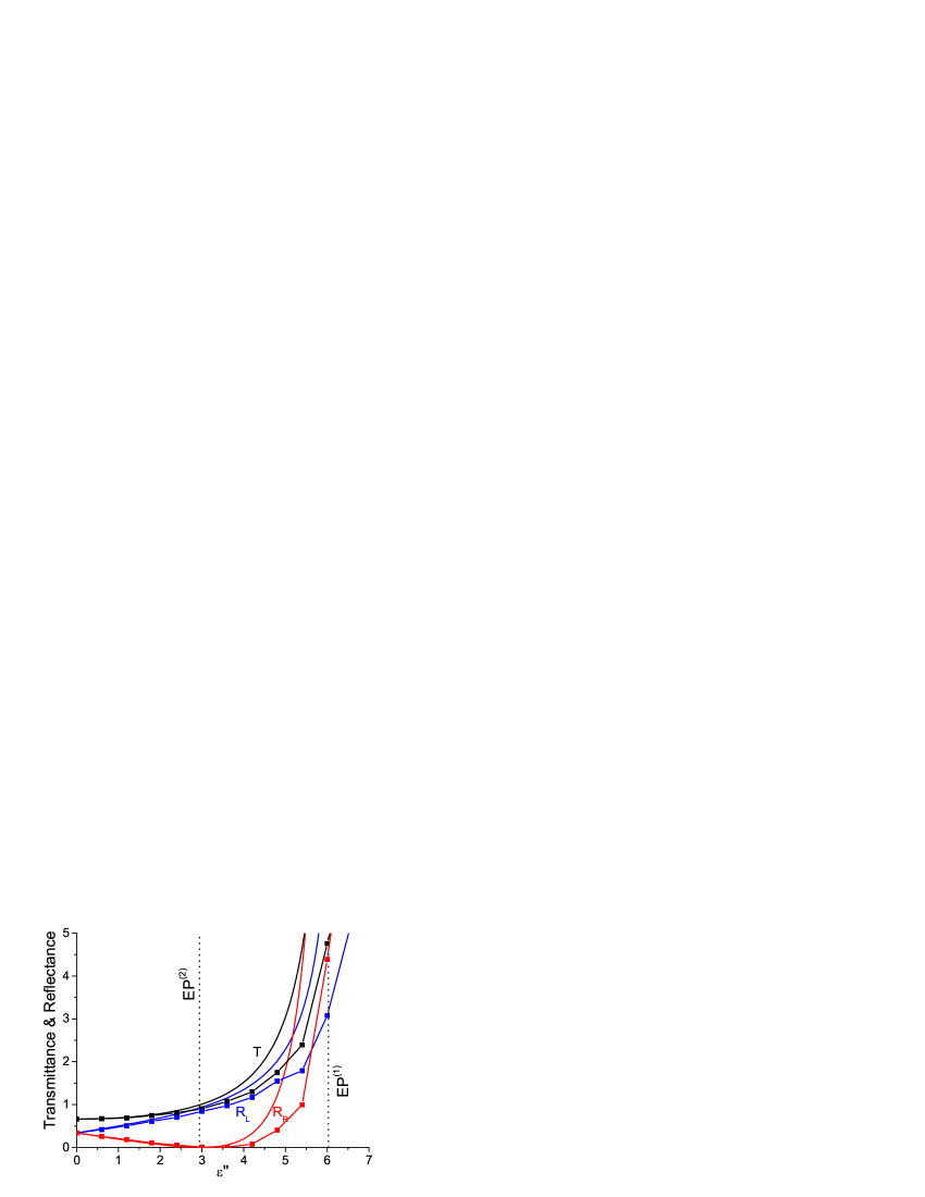
Figure 5: The same as in Fig. 3(a), but for $d=74.308$ nm (near the pole shown in Fig. 4).

Thus, the conditions of the pole appearance are not met in Fig. 3. Nevertheless, the lasinglike response is still feasible in this non-pole regime, though it requires a much stronger gain $\varepsilon^{\prime\prime}>13$ [see Fig. 3(b)] that is almost twice as large compared with the lasing at the pole. To make the difference even more clear, in Fig. 5 we plot the same quantities as in Fig. 3(a), but now at the pole. One can see that in contrast to the non-pole case, the transmittance and reflectance for the parameters corresponding to the pole show almost unbounded growth as we get closer to the EP⁽¹⁾. This is definitely associated with the lasing onset.

To explain the behavior of waves in vicinity of the pole, we will make several remarks. First, it should be noted that we deal with an external wave interacting with the gain-containing system. This implies that the frequency of the radiation is externally prescribed and amplification and instability analysis can be performed only at this single frequency. On the contrary, the “true” lasing develops from the radiation fluctuations at all frequencies, while the lasing frequency is governed by the parameters of the structure (cavity) and the gain medium. Since the pole provides the lowest instability threshold, the lasing frequency usually corresponds to the pole conditions. Second, we stress that the availability of the poles is sufficient, but not necessary for the lasing onset in the case of external irradiation considered. This is absolutely reasonable, since the poles are the geometric (zero-dimensional) points, which can be reached only with the perfect tunability of the system parameters (in our case, the precise values of the frequency and layer thickness). The instability outside the singular points is achieved in non-optimal conditions (for larger gain), so that the reflectance and transmittance of the structure are not infinite, but reach certain large enough values.

Returning to the meaning of the exceptional points, we note that the exceptional points of $\hat{S}_{1}$ allow us to approximately predict the lasing threshold, in accordance with the instability of the light propagation shown in Fig. 3(b). Since the transmittance in this case should be greater than $1$, the EP⁽¹⁾ appears at the larger $\varepsilon^{\prime\prime}$ than the EP⁽²⁾. This means that the EP⁽¹⁾ can be used as a lasing predictor, even when the conditions of a pole appearance are not fulfilled.

VI Conclusion

We have solved an important problem regarding the correct form of the scattering matrix of a photonic non-Hermitian system and, thus, determined conditions of the $\mathcal{PT}$ symmetry breaking. In particular, we have derived the scattering matrix of the 1D multilayer heterostructure unequivocally related to the $\mathcal{PT}$-symmetric Hamiltonian. It should be used for the correct prediction of the exceptional points (when transmittance $T=1$) and $\mathcal{PT}$-symmetry breaking (when $T>1$), solving the dilemma of the proper scattering matrix. Exceptional points of the scattering matrix with permuted output ports (when the sum of reflection coefficients $|r_{L}+r_{R}|=2$) are of great importance, too, since they can roughly predict the lasinglike regime. The lasing has nothing to do with the symmetry breaking, but it is related to the development of instability in the dynamic system. The described theory is not limited by the multilayer structures, but can be adapted to any non-Hermitian open system. The discussed issues might be applied for analysis of the sensing and lasing designs possessing fascinating sensibility and modal structure.

References

- (1) R.G. Newton, Scattering Theory of Waves and Particles (Springer-Verlag Berlin Heidelberg, 1982).
- (2) C. M. Bender and S. Boettcher, Real spectra in non-Hermitian Hamiltonians having symmetry, Phys. Rev. Lett. 80, 5243 (1998).
- (3) C. M. Bender, Making sense of non-Hermitian Hamiltonians, Rep. Prog. Phys. 70, 947 (2007).
- (4) A. A. Zyablovsky, A. P. Vinogradov, A. A. Pukhov, A. V. Dorofeenko, and A. A. Lisyansky, symmetry in optics, Phys. Usp. 57, 1063 (2014).
- (5) L. Feng, R. El-Ganainy, and L. Ge, Non-Hermitian photonics based on parity-time symmetry, Nat. Photon. 11, 752 (2017).
- (6) R. El-Ganainy, K. G. Makris, M. Khajavikhan, Z. H. Musslimani, S. Rotter, and D. N. Christodoulides, Non-Hermitian physics and symmetry, Nat. Phys. 13, 11 (2018).
- (7) S.K. Özdemir, S. Rotter, F. Nori, and L. Yang, Parity-time symmetry and exceptional points in photonics, Nat. Mater. 18, 783 (2019).
- (8) M.-A. Miri and A. Alu, Exceptional points in optics and photonics, Science 363, eaar7709 (2019).
- (9) C. E. Rüter, K. G. Makris, R. El-Ganainy, D. N. Christodoulides, M. Segev, and D. Kip, Observation of parity-time symmetry in optics, Nat. Phys. 6, 192 (2010).
- (10) A. Regensburger, C. Bersch, M.-A. Miri, G. Onishchukov, D.N. Christodoulides, and U. Peschel, Parity-time synthetic photonic lattices, Nature, 488, 167 (2012).
- (11) M. Kremer, T. Biesenthal, L.J. Maczewsky, M. Heinrich, R. Thomale, and A. Szameit, Demonstration of a two-dimensional -symmetric crystal, Nat. Commun. 10, 435 (2019).
- (12) L. Feng, X. Zhu, S. Yang, H. Zhu, P. Zhang, X. Yin, Y. Wang, and X. Zhang, Demonstration of a large-scale optical exceptional point structure, Opt. Express 22, 1760 (2014).
- (13) M. Lawrence, N. Xu, X. Zhang, L. Cong, J. Han, W. Zhang, and S. Zhang, Manifestation of symmetry breaking in polarization space with Terahertz metasurfaces, Phys. Rev. Lett. 113, 093901 (2014).
- (14) L. Ge, Y. D. Chong, and A. D. Stone, Conservation relations and anisotropic transmission resonances in one-dimensional -symmetric photonic heterostructures, Phys. Rev. A 85, 023802 (2012).
- (15) Z. Lin, H. Ramezani, T. Eichelkraut, T. Kottos, H. Cao, and D. N. Christodoulides, Unidirectional invisibility induced by -symmetric periodic structures, Phys. Rev. Lett. 106, 213901 (2011).
- (16) L. Feng, Y.-L. Xu, W. S. Fegadolli, M.-H. Lu, J. E. B. Oliveira, V. R. Almeida, Y.-F. Chen, and A. Scherer, Experimental demonstration of a unidirectional reflectionless paritytime metamaterial at optical frequencies, Nat. Mater. 12, 108 (2013).
- (17) A. U. Hassan, B. Zhen, M. Soljacic, M. Khajavikhan, and D. N. Christodoulides, Dynamically encircling exceptional points: Exact evolution and polarization state conversion, Phys. Rev. Lett. 118, 093002 (2017).
- (18) W. Chen, S. K. Özdemir, G. Zhao, J. Wiersig, and L. Yang, Exceptional points enhance sensing in an optical microcavity, Nature (London) 548, 192 (2017).
- (19) H. Hodaei, A. U. Hassan, S. Wittek, H. Garcia-Gracia, R. El-Ganainy, D. N. Christodoulides, and M. Khajavikhan, Enhanced sensitivity at higher-order exceptional points, Nature (London) 548, 187 (2017).
- (20) L. Feng, Z. J. Wong, R.-M. Ma, Y. Wang, and X. Zhang, Single-mode laser by parity-time symmetry breaking, Science 346, 972 (2014).
- (21) H. Hodaei, M.-A. Miri, M. Heinrich, D. N. Christodoulides, and M. Khajavikhan, Parity-time-symmetric microring lasers, Science 346, 975 (2014).
- (22) Z. Gu, N. Zhang, Q. Lyu, M. Li, S. Xiao, and Q. Song, Experimental demonstration of -symmetric stripe lasers, Laser Photon. Rev. 10, 588 (2016).
- (23) S. Longhi, -symmetric laser absorber, Phys. Rev. A 82, 031801(R) (2010).
- (24) Y. D. Chong, L. Ge, and A. D. Stone, Symmetry Breaking and Laser-Absorber Modes in Optical Scattering Systems, Phys. Rev. Lett. 106, 093902 (2011).
- (25) Z. J. Wong, Y.-L. Xu, J. Kim, K. O’Brien, Y. Wang, L. Feng, and X. Zhang, Lasing and anti-lasing in a single cavity, Nat. Photon. 10, 796 (2016).
- (26) R. Alaee, J. Christensen, and M. Kadic, Optical Pulling and Pushing Forces in Bilayer -Symmetric Structures, Phys. Rev. Appl. 9, 014007 (2018).
- (27) X. Zhou, X. Lin, Z. Xiao, T. Low, A. Alù, B. Zhang, and H. Sun, Controlling photonic spin Hall effect via exceptional points, Phys. Rev. B 100, 115429 (2019).
- (28) A. Mostafazadeh, Scattering Theory and -Symmetry, in Parity-time Symmetry and Its Applications, ed. D. Christodoulides and J. Yang (Springer, 2018), pp. 75-121.
- (29) V. Achilleos, Y. Auŕegan, and V. Pagneux, Scattering by Finite Periodic -Symmetric Structures, Phys. Rev. Lett. 119, 243904 (2017).
- (30) D.V. Novitsky, CPA-laser effect and exceptional points in -symmetric multilayer structures, J. Opt. 21, 085101 (2019).
- (31) D.V. Novitsky, A. Karabchevsky, A.V. Lavrinenko, A.S. Shalin, and A.V. Novitsky, symmetry breaking in multilayers with resonant loss and gain locks light propagation direction, Phys. Rev. B 98, 125102 (2018).
- (32) D. V. Novitsky, Femtosecond pulses in a dense two-level medium: Spectral transformations, transient processes, and collisional dynamics, Phys. Rev. A 84, 013817 (2011).
- (33) M. E. Crenshaw, Comparison of quantum and classical local-field effects on two-level atoms in a dielectric, Phys. Rev. A 78, 053827 (2008).
- (34) N. Bloembergen, Nonlinear Optics (Benjamin, New York, 1965).
- (35) D. V. Novitsky, V. R. Tuz, S. L. Prosvirnin, A. V. Lavrinenko, and A. V. Novitsky, Transmission enhancement in loss-gain multilayers by resonant suppression of reflection, Phys. Rev. B 96, 235129 (2017).
- (36) D. V. Novitsky, Compression of an intensive light pulse in photonic-band-gap structures with a dense resonant medium, Phys. Rev. A 79, 023828 (2009).
- (37) E. D. Palik (ed.), Handbook of Optical Constants of Solids (Academic Press, San Diego, 1998).
- (38) J.-C. Diels and W. Rudolph, Ultrashort Laser Pulse Phenomena (Academic Press, San Diego, 2nd edn, 2006).
- (39) Z. J. Wong, Y.-L. Xu, J. Kim, K. O’Brien, Y. Wang, L. Feng, and X. Zhang, Lasing and anti-lasing in a single cavity, Nat. Photon. 10, 796 (2016).