Riemannian Adaptive Optimization Algorithm and
Its Application to Natural Language Processing

Abstract

This paper proposes a Riemannian adaptive optimization algorithm to optimize the parameters of deep neural networks. The algorithm is an extension of both AMSGrad in Euclidean space and RAMSGrad on a Riemannian manifold. The algorithm helps to resolve two issues affecting RAMSGrad. The first is that it can solve the Riemannian stochastic optimization problem directly, in contrast to RAMSGrad which only achieves a low regret. The other is that it can use constant learning rates, which makes it implementable in practice. Additionally, we apply the proposed algorithm to Poincaré embeddings that embed the transitive closure of the WordNet nouns into the Poincaré ball model of hyperbolic space. Numerical experiments show that regardless of the initial value of the learning rate, our algorithm stably converges to the optimal solution and converges faster than the existing algorithms.

1 Introduction

Riemannian optimization has attracted a great deal of attention [7, 12, 17] in light of developments in machine learning and deep learning. This paper focuses on Riemannian adaptive optimization algorithms for solving an optimization problem on a Riemannian manifold. In the field of machine learning, there is an important example of the Riemannian optimization problem. Nickel and Kiela [13] proposed Poincaré embeddings, which embed hierarchical representations of symbolic data (e.g., text, graph data) into the Poincaré ball model of hyperbolic space. In fact, experiments on transitive closure of the WordNet noun hierarchy showed that embeddings into a 5-dimensional Poincaré ball are better than embeddings into a 200-dimensional Euclidean space. Since the Poincaré ball has a Riemannian manifold structure, the problem of finding Poincaré embeddings should be considered to be a Riemannian optimization problem.

Bonnabel [3] proposed Riemannian stochastic gradient descent (RSGD), the most basic Riemannian stochastic optimization algorithm. RSGD is a simple algorithm, but its slow convergence is problematic. In [16], Sato, Kasai, and Mishra proposed the Riemannian stochastic variance reduced gradient (RSVRG) algorithm and gave a convergence analysis under some natural assumptions. RSVRG converges to an optimal solution faster than RSGD; however, RSVRG needs to calculate the full gradient every few iterations. In Euclidean space, adaptive optimization algorithms, such as AdaGrad [4], Adam [9, Algorithm 1], Adadelta [20], and AMSGrad [14, Algorithm 2], [6, Algorithm 1], are widely used for training deep neural networks. However, these adaptive algorithms cannot be naturally extended to general Riemannian manifolds, due to the absence of a canonical coordinate system. Therefore, special measures are required to extend the adaptive algorithms to Riemannian manifolds. For instance, Kasai, Jawanpuria, and Mishra [8] proposed adaptive stochastic gradient algorithms on Riemannian matrix manifolds by adapting the row, and column subspaces of gradients.

In the particular case of a product of Riemannian manifolds, Bécigneul and Ganea [2] proposed Riemannian AMSGrad (RAMSGrad) by regarding each component of the product Riemannian manifold as a coordinate component in Euclidean space. However, their convergence analysis had two points requiring improvement. First, they only performed a regret minimization (Theorem 3.2) and did not solve the Riemannian optimization problem. Second, they did a convergence analysis with only a diminishing learning rate; i.e., they did not perform a convergence analysis with a constant learning rate. Since diminishing learning rates are approximately zero after a large number of iterations, algorithms that use them are not implementable in practice. In contrast, a constant learning rate does not cause this problem.

The motivation of this work is to identify whether or not RAMSGrad can be modified in such a way that it can be applied to Riemannian optimization from the viewpoints of both theory and practice. The theoretical motivation is to show that the modified RAMSGrad can solve directly the Riemannian optimization problem, while the practical motivation is to show that it can be applied to important problems in natural language processing and principal component analysis.

Motivated by the above discussion, we propose modified RAMSGrad (Algorithm 1), which is an extension of RAMSGrad, to solve the Riemannian optimization problem (Problem 2.1). In addition, we give a convergence analysis (Theorem 3.1) valid for both a constant learning rate (Corollary 3.1) and diminishing learning rate (Corollary 3.2). The analysis leads to the finding that the proposed algorithm can solve directly the Riemannian optimization problem. In particular, we emphasize that the proposed algorithm can use a constant learning rate to solve the problem (Corollary 3.1), in contrast to the previous result [2] in which RAMSGrad with a diminishing learning rate only performed a regret minimization (see Subsection 3.2 for comparisons of the proposed algorithm with RAMSGrad). In numerical experiments, we apply the proposed algorithm to Poincaré embeddings and compare it with RSGD, Riemannian AdaGrad (RAdaGrad) [2, Section 3.2], and Riemannian Adam (RAdam) [2, Section 4] (Section 4). We show that it converges to the optimal solution faster than the existing algorithms and that it minimizes the objective function regardless of the initial learning rate. In particular, we show that the proposed algorithm with a constant learning rate is a good way of embedding the WordNet mammals subtree into a Poincaré ball. We also applied the algorithm to principal component analysis and found that the choice between using a constant or a diminishing learning rate depends on the dataset. These numerical comparisons lead to the finding that the proposed algorithm is good for solving important problems in natural language processing and principal component analysis.

This paper is organized as follows. Section 2 gives the mathematical preliminaries and states the main problem. Section 3 describes the modified RAMSGrad and gives its convergence analysis. Section 4 numerically compares the performance of the proposed learning algorithms with the existing algorithms. Section 5 concludes the paper with a brief summary.

2 Mathematical Preliminaries

2.1 Definitions, assumptions, and main problem

Let $M$ be a Riemannian manifold. An exponential map at $x\in M$, written as $\exp_{x}\colon T_{x}M\rightarrow M$, is a mapping from the tangent space $T_{x}M$ to $M$ with the requirement that a vector $\xi\in T_{x}M$ is mapped to the point $y:=\exp_{x}(\xi)\in M$ such that there exists a geodesic $\gamma\colon[0,1]\rightarrow M$, which satisfies $\gamma(0)=x$, $\gamma(1)=y$, and $\dot{\gamma}(0)=\xi$, where $\dot{\gamma}$ is the derivative of $\gamma$ (see [1, 21]). Moreover, $\log_{x}\colon M\rightarrow T_{x}M$ denotes a logarithmic map at a point $x\in M$, which is defined as the inverse mapping of the exponential map at $x\in M$. For all $x,y\in M$, the existence of $\log_{x}(y)$ is guaranteed [15, Chapter V, Theorem 4.1] [11, Proposition 2.1].

Next, we give the definitions of a geodesically convex set and function (see [21, Section 2]) that generalize the concepts of a convex set and function in Euclidean space.

Definition 2.1 (Geodesically convex set).

Let $X$ be a subset of a Riemannian manifold $M$. $X$ is said to be geodesically convex if, for any two points in $X$, there is a unique minimizing geodesic within $X$ which joins those two points.

Definition 2.2 (Geodesically convex function).

A smooth function $f\colon M\rightarrow\mathbb{R}$ is said to be geodesically convex if, for any $x,y\in M$, it holds that

$$f(y)\geq f(x)+\left\langle{\operatorname*{grad}{f(x)},\log_{x}(y)}\right\rangle_{x},$$

where $\left\langle{\cdot,\cdot}\right\rangle_{x}$ is the Riemannian metric on $M$, and $\operatorname*{grad}f(x)$ is the Riemannian gradient of $f$ at a point $x\in M$ (see [1]).

For $i\in\{1,2,\cdots,N\}$, let $M_{i}$ be a Riemannian manifold and $M$ be the Cartesian product of $n$ Riemannian manifolds $M_{i}$ (i.e., $M:=M_{1}\times\cdots\times M_{N}$). $x^{i}\in M_{i}$ denotes a corresponding component of $x\in M$, and $\left\langle{\cdot,\cdot}\right\rangle_{x^{i}}$ denotes a Riemannian metric at a point $x^{i}\in M_{i}$. Furthermore, $\left\lVert{\cdot}\right\rVert_{x^{i}}$ represents the norm determined from the Riemann metric $\left\langle{\cdot,\cdot}\right\rangle_{x^{i}}$. For a geodesically convex set $X_{i}\subset M_{i}$, we define the projection operator as $\Pi_{X_{i}}:M_{i}\rightarrow X_{i}$; i.e., $\Pi_{X_{i}}(x^{i})$ is the unique point $y^{i}\in X_{i}$ minimizing $d^{i}(x^{i},\cdot)$, where $d^{i}(\cdot,\cdot):M_{i}\times M_{i}\rightarrow\mathbb{R}$ denotes the distance function of $M_{i}$. The tangent space at a point $x=(x^{1},x^{2},\cdots,x^{N})\in M$ is given by $T_{x}M=T_{x^{1}}M_{1}\oplus\cdots\oplus T_{x^{N}}M_{N}$, by considering $T_{x^{i}}M_{i}$ to be a subspace of $T_{x}M$, where $\oplus$ is the direct sum of vector spaces. Then, for a point $x=(x^{1},x^{2},\cdots,x^{N})\in M$ and a tangent vector $\xi\in T_{x}M$, we write $\xi=(\xi^{i})=(\xi^{1},\xi^{2},\cdots,\xi^{N})$, where $i\in\{1,2\cdots,N\}$, and $\xi^{i}\in T_{x^{i}}M_{i}$. Finally, for $x^{i},y^{i}\in M_{i}$, $\varphi_{x^{i}\rightarrow y^{i}}^{i}$ denotes an isometry from $T_{x^{i}}M_{i}$ to $T_{y^{i}}M_{i}$ (e.g., $\varphi^{i}_{x^{i}\rightarrow y^{i}}$ stands for parallel transport from $T_{x^{i}}M_{i}$ to $T_{y^{i}}M_{i}$).

$\mathbb{E}\left[{X}\right]$ denotes the expectation of a random variable $X$, and $t_{[n]}$ denotes the history of the process up to time $n$ (i.e., $t_{[n]}:=(t_{1},t_{2},\cdots,t_{n})$). $\mathbb{E}[X|t_{[n]}]$ denotes the conditional expectation of $X$ given $t_{[n]}$.

Assumption 2.1.

For $i\in\{1,2,\cdots,N\}$, let $M_{i}$ be a complete simply connected Riemannian manifold with sectional curvature lower bounded by $\kappa_{i}\leq 0$. We define $M:=M_{1}\times\cdots\times M_{N}$. Then, we assume

(A1)

For all $i\in\{1,2,\cdots,N\}$, let $X_{i}\subset M_{i}$ be a bounded, closed, geodesically convex set and $X:=X_{1}\times\cdots\times X_{N}$. In addition, $X_{i}\subset M_{i}$ has a diameter bounded by $D$; i.e., there exists a positive real number $D$ such that

$$\max_{i\in\{1,2,\cdots,N\}}\sup\{d^{i}(x^{i},y^{i}):x^{i},y^{i}\in X_{i}\}\leq D,$$

where $d^{i}(\cdot,\cdot)$ denotes the distance function of $M_{i}$;

(A2)

A smooth function $f_{t}:M\rightarrow\mathbb{R}$ is geodesically convex, where $t$ is a random variable whose probability distribution is a uniform distribution and supported on a set $\mathcal{T}:=\{1,2,\cdots,T\}$. The function $f$ is defined for all $x\in M$, by $f(x):=\mathbb{E}\left[{f_{t}(x)}\right]=(1/T)\sum_{t=1}^{T}f_{t}(x)$.

Note that, when we define a positive number $G$ as

$$G:=\sup_{t\in\mathcal{T},x\in X}\left\lVert{\operatorname*{grad}f_{t}(x)}\right\rVert_{x},$$

we find that $G<\infty$ from Assumption 2.1 (A1). The following is the main problem considered here [2, Section 4]:

Problem 2.1.

Suppose that Assumption 2.1 holds. Then, we have

$$x_{\ast}\in X_{\ast}:=\left\{x_{\ast}\in X:f(x_{\ast})=\inf_{x\in X}f(x)\right\}.$$

2.2 Background and motivation

Euclidean adaptive optimization algorithms, such as AdaGrad, Adam, and AMSGrad, are powerful tools for training deep neural networks. However, there are optimization problems on Riemannian manifolds in machine learning [13] that cannot be solved by Euclidean adaptive optimization algorithms. Accordingly, useful algorithms, such as RSGD [3, Section 2], RAdaGrad [2, Section 3.2], RAdam [2, Section 4], and RAMSGrad [2, Figure 1(a)], have been developed to solve Riemannian optimization problems. The algorithms, such as RAdaGrad, RAdam, and RAMSGrad, are based on the Euclidean adaptive optimization algorithms, AdaGrad, Adam, and AMSGrad. Hence, we can expect that the corresponding Riemannian adaptive optimization algorithms perform better than RSGD, the most basic Riemannian stochastic optimization algorithm. In fact, the numerical comparisons in [2] showed that Riemannian adaptive optimization algorithms are superior for the task of embedding the WordNet taxonomy in the Poincaré ball.

Although Riemannian adaptive optimization algorithms have been shown to be useful for Riemannian optimization in machine learning, we have two motivations related to the previous results in [2]. The first motivation is to identify whether or not RAMSGrad can solve directly the Riemannian optimization problem. This is because the previous results in [2] only showed that RAMSGrad performs a regret minimization, which does not lead to Riemannian minimization (see Subsection 3.2 for details). The second motivation is to identify whether or not RAMSGrad is applicable to significant problems in fields such as natural language processing and principal component analysis. This is because the previous results in [2] only gave a convergence analysis of RAMSGrad with a diminishing learning rate. Diminishing learning rates are approximately zero after a large number of iterations, which implies that algorithms with them are not implementable in practice. In contrast, a constant learning rate does not cause this problem (see Subsection 3.2 for details).

Therefore, our goal is to devise an algorithm that overcomes the above issues. In particular, the following section proposes an adaptive optimization algorithm (Algorithm 1) with a constant learning rate that can solve Problem 2.1 directly (Corollary 3.1).

3 Riemannian Adaptive Optimization Algorithm

3.1 Proposed algorithm and its convergence analysis

We propose the following algorithm (Algorithm 1). A small constant $\epsilon>0$ in the definition of $\hat{v}_{n}^{i}$ guarantees that $\sqrt{\hat{v}_{n}^{i}}>0$ (Adam [9, Algorithm 1] and AMSGrad [14, Algorithm 2], [6, Algorithm 1] use such a constant in practice).

Algorithm 1 Modified RAMSGrad for solving Problem 2.1

0:  $(\alpha_{n})_{n\in\mathbb{N}}\subset[0,1),(\beta_{1n})_{n\in\mathbb{N}}\subset[0,1),\beta_{2}\in[0,1),\epsilon>0$

1:  $n\leftarrow 1,x_{1}\in X,\tau_{0}=m_{0}=0\in T_{x_{0}}M,v_{0}^{i},\hat{v}_{0}^{i}=0\in\mathbb{R}$

2:  loop

3:     $g_{t_{n}}=(g_{t_{n}}^{i})=\operatorname*{grad}{f_{t_{n}}(x_{n})}$

4:     for $i=1,2,\cdots,N$ do

5:        $m_{n}^{i}=\beta_{1n}\tau_{n-1}^{i}+(1-\beta_{1n})g_{t_{n}}^{i}$

6:        $v_{n}^{i}=\beta_{2}v_{n-1}^{i}+(1-\beta_{2})\left\lVert{g_{t_{n}}^{i}}\right\rVert_{x_{n}^{i}}^{2}$

7:        $\hat{v}_{n}^{i}=\max\{\hat{v}_{n-1}^{i},v_{n}^{i}\}+\epsilon$

8:        $x_{n+1}^{i}=\Pi_{X_{i}}\left[\exp_{x_{n}^{i}}^{i}\left(-\alpha_{n}\dfrac{m_{n}^{i}}{\sqrt{\hat{v}_{n}^{i}}}\right)\right]$

9:        $\tau_{n}^{i}=\varphi_{x_{n}^{i}\rightarrow x_{n+1}^{i}}^{i}(m_{n}^{i})$

10:     end for

11:     $n\leftarrow n+1$

12:  end loop

Now, let us compare Algorithm 1 on a Riemannian manifold with AMSGrad in Euclidean space. For simplicity, let us suppose that $M_{i}=X_{i}=\mathbb{R}$ ($i=1,2,\ldots,N$). Then, Algorithm 1 defined on $M=\mathbb{R}^{N}$ is as follows: given $\bm{x}_{1}\in\mathbb{R}^{N}$ and $\bm{m}_{0}=\bm{v}_{0}=\hat{\bm{v}}_{0}=\bm{0}\in\mathbb{R}^{N}$,

$$\bm{m}_{n}=\beta_{1n}\bm{m}_{n-1}+(1-\beta_{1n})\bm{g}_{t_{n}},$$

$$\bm{v}_{n}=\beta_{2}\bm{v}_{n-1}+(1-\beta_{2})\bm{g}_{t_{n}}\odot\bm{g}_{t_{n}},$$

$$\hat{\bm{v}}_{i}=(\hat{v}_{n}^{i})_{i}=\left(\max\left\{\hat{v}_{n-1}^{i},v_{n}^{i}\right\}+\epsilon\right)_{i},$$

$$\bm{x}_{n+1}=\left(x_{n}^{i}-\alpha_{n}\frac{m_{n}^{i}}{\sqrt{\hat{v}_{n}^{i}}}\right)_{i},$$

where $\bm{x}\odot\bm{x}:=({x^{i}}^{2})_{i}$ for $\bm{x}=(x^{i})_{i}\in\mathbb{R}^{N}$. This implies Algorithm 1 is an extension of AMSGrad.

Our convergence analysis (Theorem 3.1) allows Algorithm 1 to use both constant and diminishing learning rates. Corollaries 3.1, and 3.2 are convergence analyses of Algorithm 1 with constant and diminishing learning rates, respectively.

Theorem 3.1.

Suppose that Assumption 2.1 holds. Let $(x_{n})_{n\in\mathbb{N}}$ and $(\hat{v}_{n})_{n\in\mathbb{N}}$ be the sequences generated by Algorithm 1. We assume $\beta_{1n}\leq\beta_{1,n-1}$ for all $n\in\mathbb{N}$, and $(\alpha_{n})_{n\in\mathbb{N}}$ is a sequence of positive learning rates, which satisfies $\alpha_{n}(1-\beta_{1n})\leq\alpha_{n-1}(1-\beta_{1,n-1})$ for all $n\in\mathbb{N}$. We define $G:=\max_{t\in\mathcal{T},x\in X}\left\lVert{\operatorname*{grad}f_{t}(x)}\right\rVert_{x}$. Then, for all $x_{\ast}\in X_{\ast}$,

$$\begin{split}~{}&\mathbb{E}\left[{\frac{1}{n}\sum_{k=1}^{n}f(x_{k})-f(x_{\ast})}\right]\\ &\leq\dfrac{NGD^{2}}{2(1-\beta_{11})}\frac{1}{n\alpha_{n}}+\dfrac{G^{2}}{2\sqrt{\epsilon}(1-\beta_{11})}\sum_{i=1}^{N}\zeta(\kappa_{i},D)\frac{1}{n}\sum_{k=1}^{n}\alpha_{k}\\ &\quad+\frac{NGD}{1-\beta_{11}}\frac{1}{n}\sum_{k=1}^{n}\beta_{1k},\end{split}$$ (1)

where $\zeta(\kappa_{i},D)$ is defined as in Lemma A.1.

Proof.

See Appendix B. ∎

Corollary 3.1 (Constant learning rate).

Suppose that the assumptions in Theorem 3.1 hold, $\alpha_{n}:=\alpha>0$, and $\beta_{1n}:=\beta\in[0,1)$. Then, Algorithm 1 satisfies, for all $x_{\ast}\in X_{\ast}$,

$$\mathbb{E}\left[{\frac{1}{n}\sum_{k=1}^{n}f(x_{k})-f(x_{\ast})}\right]\leq\mathcal{O}\left(\frac{1}{n}\right)+C_{1}\alpha+C_{2}\beta,$$

where $C_{1},C_{2}>0$ are constants.

Proof.

See Appendix C. ∎

Corollary 3.2 (Diminishing learning rate).

Suppose that the assumptions in Theorem 3.1 hold, $\alpha_{n}:=1/n^{\eta}$, where $\eta\in[1/2,1)$, and $\sum_{k=1}^{\infty}\beta_{1k}<\infty$ . Then, Algorithm 1 satisfies, for all $x_{\ast}\in X_{\ast}$,

$$\mathbb{E}\left[{\frac{1}{n}\sum_{k=1}^{n}f(x_{k})-f(x_{\ast})}\right]=\mathcal{O}\left(\dfrac{1}{n^{1-\eta}}\right).$$

Proof.

See Appendix C. ∎

3.2 Comparison of Algorithm 1 with the existing algorithms

Algorithm 1 with $n=t\in\mathcal{T}$ coincides with RAMSGrad [2, Figure 1(a)]. In [2], Bécigneul and Ganea used “regret” to guarantee the convergence of RAMSGrad. The regret at the end of $T$ iterations is defined as

$$R_{T}:=\sum_{t\in\mathcal{T}}f_{t}(x_{t})-f_{*},$$

where $(f_{t})_{t\in\mathcal{T}}$ is a family of differentiable, geodesically convex functions from $M$ to $\mathbb{R}$, $f_{*}:=\min_{x\in X}\sum_{t\in\mathcal{T}}f_{t}(x)$, and $(x_{t})_{t\in\mathcal{T}}$ is the sequence generated by RAMSGrad. They proved the following theorem [2, Theorem 1]:

Theorem 3.2 (Convergence of RAMSGrad).

Suppose that Assumption 2.1 (A1) holds and that $f_{t}$ is smooth and geodesically convex for all $t\in\mathcal{T}$. Let $(x_{t})_{t\in\mathcal{T}}$ and $(\hat{v}_{t})_{t\in\mathcal{T}}$ be the sequences obtained from RAMSGrad, $\alpha_{t}=\alpha/\sqrt{t}$, $\beta_{1}=\beta_{11}$, $\beta_{1k}\leq\beta_{1}$ for all $t\in\mathcal{T}$, $\alpha>0$, and $\gamma:=\beta_{1}/\sqrt{\beta_{2}}<1$. We then have:

$$R_{T}\leq\frac{\sqrt{T}D^{2}}{2\alpha(1-\beta_{1})}\sum_{i=1}^{N}\sqrt{\hat{v}_{T}^{i}}+\frac{D^{2}}{2(1-\beta_{1})}\sum_{i=1}^{N}\sum_{t=1}^{T}\beta_{1t}\dfrac{\sqrt{\hat{v}_{t}^{i}}}{\alpha_{t}}$$

$$+\frac{\alpha\sqrt{1+\log{T}}}{(1-\beta_{1})^{2}(1-\gamma)\sqrt{1-\beta_{2}}}\sum_{i=1}^{N}\frac{\zeta(\kappa_{i},D)+1}{2}\sqrt{\sum_{t=1}^{T}\left\lVert{g_{t}^{i}}\right\rVert_{x_{t}^{i}}^{2}}.$$

Note that Theorem 3.2 asserts the regret generated by RAMSGrad has an upper bound. We should also note that regret minimization does not always lead to solutions of Problem 2.1. This is because, even if $(x_{t})_{t\in\mathcal{T}}$ satisfies, for a sufficiently large number $T$,

$$R_{T}=\sum_{t\in\mathcal{T}}f_{t}(x_{t})-f_{*}\approx 0,$$

and we do not have that

$$Tf(x_{T})-f_{*}=\sum_{t\in\mathcal{T}}f_{t}(x_{T})-f_{*}\approx 0.$$

Accordingly, Theorem 3.2 does not guarantee that the output $x_{T}$ generated by RAMSGrad approximates the solution of Problem 2.1. Additionally, Theorem 3.2 assumes a diminishing learning rate $\alpha_{t}$ and does not assert anything about a constant learning rate.

Meanwhile, Corollary 3.1 implies that, if we use sufficiently small constant learning rates $\alpha$ and $\beta$, then Algorithm 1 satisfies

$$\mathbb{E}\left[{\frac{1}{n}\sum_{k=1}^{n}f(x_{k})-f_{*}}\right]\leq\mathcal{O}\left(\frac{1}{n}\right)+C_{1}\alpha+C_{2}\beta\approx\mathcal{O}\left(\frac{1}{n}\right),$$

which implies that Algorithm 1 approximates the solution of Problem 2.1 in the sense of the mean value of $f(x_{k})$. Although Theorem 3.2 can only use diminishing learning rates such that $\alpha_{t}:=\alpha/\sqrt{t}$, Corollary 3.1 guarantees that Algorithm 1 with a constant learning rate can solve Problem 2.1.

Corollary 3.2 implies that Algorithm 1 with a diminishing learning rate can solve Problem 2.1 in the sense that

$$\mathbb{E}\left[{\frac{1}{n}\sum_{k=1}^{n}f(x_{k})-f_{*}}\right]=\mathcal{O}\left(\dfrac{1}{n^{1-\eta}}\right),$$

while Theorem 3.2 implies that RAMSGrad only minimizes the regret in the sense of the existence of a positive real number $C$ such that

$$\frac{R_{T}}{T}\leq C\sqrt{\frac{1+\log{T}}{T}}.$$

Additionally, Theorem 3.2 implies RAMSGrad only works in the case where $\eta=1/2$, but Corollary 3.2 implies Algorithm 1 works for a wider range of $\eta$.

The advantage of Corollary 3.2 over Corollary 3.1 is that using a diminishing learning rate is a robust way to solve Problem 2.1. However, it is possible that Algorithm 1 with a diminishing learning rate does not work for a sufficiently large number $S$ of iterations, because step 8 in Algorithm 1 with $\alpha_{S}\approx 0$ satisfies

$$x_{S+1}^{i}=\Pi_{X_{i}}\left[\exp_{x_{S}^{i}}^{i}\left(-\alpha_{S}\dfrac{m_{S}^{i}}{\sqrt{\hat{v}_{S}^{i}}}\right)\right]\approx x_{S}^{i}.$$

Such a trend was observed in [6]. The numerical results in [6] showed that Euclidean adaptive optimization algorithms, such as Adam and AMSGrad, with constant learning rates (e.g., $\alpha_{n}=\beta_{1n}=10^{-3}$) perform better than those with diminishing ones in terms of both the training loss and accuracy score. Moreover, we can see that the Euclidean adaptive optimization algorithms in torch.optim use constant learning rates, such as $\alpha_{n}=10^{-3}$ and $\beta_{1n}=0.9,0.999$.

According to [3, Section 2] and [2, Section 5], useful constant learning rates in RAMSGrad are $\alpha_{n}=0.3,0.1$ and $\beta_{1n}=0.9$. Meanwhile, Corollary 3.1 indicates that using a small constant learning rate $\beta_{1n}$ would be good for solving Problem 2.1. Accordingly, the next section numerically compares the behavior of Algorithm 1 with $\beta_{1n}=0.9$ with one with $\beta_{1n}=0.001<0.9$. Corollary 3.2 (see also Theorem 3.2) indicates that Algorithm 1 should use diminishing learning rates such that $\alpha_{n}=\mathcal{O}(1/\sqrt{n})$ and $\beta_{1n}=\lambda^{n}$ ($\lambda\in[0,1)$). The next section uses diminishing learning rates to compare fairly the behaviors of Algorithm 1 with constant learning rates (see Section 4 for details).

4 Numerical Experiments

We numerically compared the following Riemannian stochastic optimization algorithms: RSGD [3, Section 2], RAdaGrad [2, Section 3.2], RAdam [2, Section 4], and Algorithm 1 (modified RAMSGrad). RAdam is obtained by removing the $\max$ operation in Algorithm 1, i.e., replacing $\hat{v}_{n}^{i}=\max\{\hat{v}_{n-1}^{i},v_{n}^{i}\}+\epsilon$ with $\hat{v}_{n}^{i}=v_{n}^{i}+\epsilon$ (see [2]). Our experiments were conducted on a fast scalar computation server at Meiji University. The environment has two Intel(R) Xeon(R) Gold 6148 (2.4 GHz, 20 cores) CPUs, an NVIDIA Tesla V100 (16GB, 900Gbps) GPU and a Red Hat Enterprise Linux 7.6 operating system.

4.1 Poincaré embeddings

In [13], Nickel and Kiela developed Poincaré embeddings. Before describing the numerical experiments, we will review the fundamentals of hyperbolic geometry (see [13, 18, 5, 2]). $\mathcal{B}^{d}:=\{x\in\mathbb{R}^{d}:\left\lVert{x}\right\rVert<1\}$ denotes the open $d$-dimensional unit ball, where $\left\lVert{\cdot}\right\rVert$ denotes the Euclidean norm. The Poincaré ball model of hyperbolic space $(\mathcal{B}^{d},\rho)$ is defined by a manifold $\mathcal{B}^{d}$ equipped with the following Riemannian metric:

$$\rho_{x}:=\frac{4}{(1-\left\lVert{x}\right\rVert^{2})^{2}}\rho^{E}_{x},$$

where $x\in\mathcal{B}^{d}$, and $\rho^{E}_{x}$ denotes the Euclidean metric tensor. The Riemannian manifold $(\mathcal{B}^{d},\rho)$ has a constant sectional curvature, $-1$. We define Möbius addition [18, Definition 1.10] of $x$ and $y$ in $\mathcal{B}^{d}$ as

$$x\oplus_{M}y:=\frac{(1+2\left\langle{x,y}\right\rangle+\left\lVert{y}\right\rVert^{2})x+(1-\left\lVert{x}\right\rVert^{2})y}{1+2\left\langle{x,y}\right\rangle+\left\lVert{x}\right\rVert^{2}\left\lVert{y}\right\rVert^{2}},$$

where $\left\langle{\cdot,\cdot}\right\rangle:=\rho^{E}(\cdot,\cdot)$. Moreover, $\ominus_{M}x$ denotes the left inverse [18, Definition 1.7] of $x\in\mathcal{B}^{d}$, and the Möbius gyrations [18, Definition 1.11] of $\mathcal{B}^{d}$ are defined as

$$\textrm{gyr}[x,y]z:=\ominus_{M}(x\oplus_{M}y)\oplus_{M}\{x\oplus_{M}(y\oplus_{M}z)\},$$

for all $x,y,z\in\mathcal{B}^{d}$.

In accordance with the above statements, the induced distance function on $(\mathcal{B}^{d},\rho)$ (see [5, Eq. (6)]) is defined for all $x,y\in\mathcal{B}^{d}$, by

$$~{}d(x,y)=2\tanh^{-1}\left(\left\lVert{(-x)\oplus_{M}y}\right\rVert\right).$$ (2)

The exponential map on $(\mathcal{B}^{d},\rho)$ (see [5, Lemma 2]) is expressed as follows: for $x\in\mathcal{B}^{d}$ and $\xi\neq 0\in T_{x}\mathcal{B}^{d}$,

$$\exp_{x}(\xi)=x\oplus_{M}\left\{\tanh\left(\frac{\left\lVert{\xi}\right\rVert}{1-\left\lVert{x}\right\rVert^{2}}\right)\right\}\frac{\xi}{\left\lVert{\xi}\right\rVert},$$

and, for $x\in\mathcal{B}^{d}$ and $0\in T_{x}\mathcal{B}^{d}$,

$$\exp_{x}(0)=x.$$

Parallel transport of $(\mathcal{B}^{d},\rho)$ (see [2, Section 5]) along the unique geodesic from $x$ to $y$ is given by

$$\varphi_{x\rightarrow y}(\xi)=\frac{1-\left\lVert{y}\right\rVert^{2}}{1-\left\lVert{x}\right\rVert^{2}}\textrm{gyr}[y,-x]\xi.$$

The Riemannian gradient on $(\mathcal{B}^{d},\rho)$ (see [2, Section 5]) is expressed in terms of rescaled Euclidean gradients, i.e., for $x\in\mathcal{B}^{d}$, and the smooth function $f:\mathcal{B}^{d}\rightarrow\mathbb{R}$,

$$\operatorname*{grad}{f(x)}=\frac{(1-\left\lVert{x}\right\rVert^{2})^{2}}{4}\nabla^{E}f(x),$$

where $\nabla^{E}f(x)$ denotes the Euclidean gradient of $f$.

To compute the Poincaré embeddings for a set of $N$ symbols by finding the embeddings $\Theta=\{u_{i}\}_{i=1}^{N}$, where $u_{i}\in\mathcal{B}^{d}$, we solve the following optimization problem: given $\mathcal{L}:\mathcal{B}^{d}\times\cdots\times\mathcal{B}^{d}\rightarrow\mathbb{R}$,

$$~{}\textrm{minimize }\mathcal{L}(\Theta)\quad\textrm{subject to }u_{i}\in\mathcal{B}^{d}.$$ (3)

The transitive closure of the WordNet mammals subtree consists of 1,180 nouns and 6,450 hypernymy Is-A relations. Let $\mathcal{D}=\{(u,v)\}$ be the set of observed hypernymy relations between noun pairs. We minimize a loss function defined by

$$~{}\mathcal{L}(\Theta)=\sum_{(u,v)\in\mathcal{D}}\log{\dfrac{e^{-d(u,v)}}{\sum_{v^{\prime}\in\mathcal{N}(u)}e^{-d(u,v^{\prime})}}},$$ (4)

where $d(u,v)$ defined by (2) is the corresponding distance of the relation $(u,v)\in\mathcal{D}$, and $\mathcal{N}(u)=\{v^{\prime}:(u,v^{\prime})\not\in\mathcal{D}\}\cup\{v\}$ is the set of negative examples for $u$ including $v$ (see [2, 13]). We embed the transitive closure of the WordNet mammals subtree into a $5$-dimensional Poincaré ball $(\mathcal{B}^{5},\rho)$.

Let us define $M_{i}:=\mathcal{B}^{5}$ and $X_{i}:=\{x\in\mathcal{B}^{5}:\left\lVert{x}\right\rVert\leq 1-10^{-5}\}$, whose projection operator $\Pi_{X_{i}}:\mathcal{B}^{5}\rightarrow X_{i}$ is computed as

$$\Pi_{X_{i}}(x):=\begin{cases}x&\textrm{if }\left\lVert{x}\right\rVert\leq 1-10^{-5}\\ (1-10^{-5})\dfrac{x}{\left\lVert{x}\right\rVert}&\textrm{otherwise}\end{cases}.$$

Moreover, the geodesically convex set $X_{i}$ has a bounded diameter; in fact, let $D$ be the diameter of a closed disk $X_{i}$, measured by the Riemann metric of $\rho$.

As in [13], we will introduce an index for evaluating the embedding. For each observed relation $(u,v)\in\mathcal{D}$, we compute the corresponding distance $d(u,v)$ in the embedding and rank it among the set of negative relations for $u$, i.e., among the set $\{d(u,v^{\prime}):(u,v^{\prime})\not\in\mathcal{D}\}$. In addition, we assume the reconstruction setting (see [13]); i.e., we evaluate the ranking of all nouns in the dataset. Then, we record the mean rank of $v$ as well as the mean average precision (MAP) of the ranking. Thus, we evaluate the embedding in terms of the loss function values and the MAP rank.

We experimented with a special iteration called the “burn-in phase” (see [13, Section 3]) for the first 20 epochs. During the burn-in phase, the algorithm runs at a reduced learning rate of $1/100$. When we minimized the loss function (4), we randomly sampled 10 negative relations per positive relation. We set $\epsilon=10^{-8}$ in Algorithm 1.

The experiment used the code of Facebook Research, and we used the NumPy 1.17.3 package and PyTorch 1.3.0 package.

4.1.1 Constant learning rate

First, we compared algorithms with the following ten constant learning rates:

(CS1)

RSGD: $\alpha_{n}=0.3$.

(CS2)

RSGD: $\alpha_{n}=0.1$.

(CG1)

RAdaGrad: $\alpha_{n}=0.3$.

(CG2)

RAdaGrad: $\alpha_{n}=0.1$.

(CD1)

RAdam: $\alpha_{n}=0.3$, $\beta_{1n}=0.9$, $\beta_{2}=0.999$.

(CD2)

RAdam: $\alpha_{n}=0.1$, $\beta_{1n}=0.9$, $\beta_{2}=0.999$.

(CA1)

Algorithm 1: $\alpha_{n}=0.3$, $\beta_{1n}=0.9$, $\beta_{2}=0.999$.

(CA2)

Algorithm 1: $\alpha_{n}=0.3$, $\beta_{1n}=0.001$, $\beta_{2}=0.999$.

(CA3)

Algorithm 1: $\alpha_{n}=0.1$, $\beta_{1n}=0.9$, $\beta_{2}=0.999$.

(CA4)

Algorithm 1: $\alpha_{n}=0.1$, $\beta_{1n}=0.001$, $\beta_{2}=0.999$.

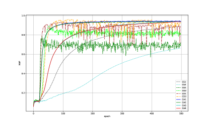
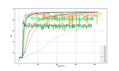
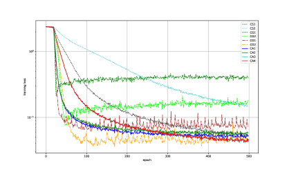
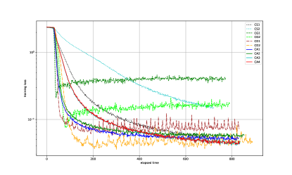
The parameter $\alpha_{n}$ in (CS1) and (CS2) represents the learning rate of RSGD [3, Section 2]. The learning rates of (CA1)–(CA4) satisfy the assumptions of Corollary 3.1. The parameters $\beta_{2}=0.999$ and $\beta_{1n}=0.9$ in (CA1) and (CA3) are used in [2, Section 5]. We used $\beta_{1n}=0.001$ in (CA2) and (CA4) to compare (CA1) and (CA3) with Algorithm 1 with a small learning rate. Figs. 1–4 show the numerical results. Fig. 1 shows the performances of the algorithms for loss function values defined by (4) with respect to the number of epochs, while Fig. 2 presents those with respect to the elapsed time. Fig. 3 shows the MAP ranks of the embeddings with respect to the number of epochs, while Fig. 4 presents the MAP ranks with respect to the elapsed time. We can see that Algorithm 1 outperforms RSGD and RAdaGrad in every setting. In particular, Figs. 1–2 show that the learning outcomes of RSGD fluctuate greatly depending on the learning rate. In contrast, Algorithm 1 and RAdam eventually reduce the loss function the most for any learning rate. Moreover, these figures show that the performance of (CA1) (resp. (CA3)) is comparable to that of (CA2) (resp. (CA4)). Meanwhile, RAdaGrad quickly reduced the objective function value in the early stages; however, it soon stopped learning.

Figure 1: Loss function value versus number of epochs in the case of constant learning rates.

Figure 2: Loss function value versus elapsed time in the case of constant learning rates.

Figure 3: MAP rank versus number of epochs in the case of constant learning rates.

Figure 4: MAP rank versus elapsed time in the case of constant learning rates.

4.1.2 Diminishing learning rate

Next, we compared algorithms with the following ten diminishing learning rates:

(DS1)

RSGD: $\alpha_{n}=30/\sqrt{n}$.

(DS2)

RSGD: $\alpha_{n}=10/\sqrt{n}$.

(DG1)

RAdaGrad: $\alpha_{n}=30/\sqrt{n}$.

(DG2)

RAdaGrad: $\alpha_{n}=10/\sqrt{n}$.

(DD1)

RAdam: $\alpha_{n}=30/\sqrt{n}$, $\beta_{1n}=0.5^{n}$, $\beta_{2}=0.999$.

(DD2)

RAdam: $\alpha_{n}=10/\sqrt{n}$, $\beta_{1n}=0.5^{n}$, $\beta_{2}=0.999$.

(DA1)

Algorithm 1: $\alpha_{n}=30/\sqrt{n}$, $\beta_{1n}=0.5^{n}$, $\beta_{2}=0.999$.

(DA2)

Algorithm 1: $\alpha_{n}=30/\sqrt{n}$, $\beta_{1n}=0.9^{n}$, $\beta_{2}=0.999$.

(DA3)

Algorithm 1: $\alpha_{n}=10/\sqrt{n}$, $\beta_{1n}=0.5^{n}$, $\beta_{2}=0.999$.

(DA4)

Algorithm 1: $\alpha_{n}=10/\sqrt{n}$, $\beta_{1n}=0.9^{n}$, $\beta_{2}=0.999$.

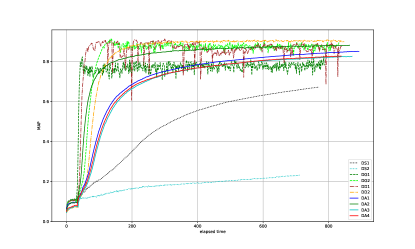
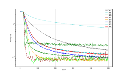
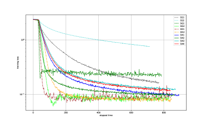
The learning rates of (DA1)–(DA4) satisfy the assumptions of Corollary 3.2. We implemented (DA2) and (DA4) to compare them with (CA1) and (CA3). We implemented (DA1) and (DA3) to check how well Algorithm 1 works depending on the choice of $\beta_{1n}$. Figs. 5–8 show the numerical results. Fig. 5 shows the behaviors of the algorithms for loss function values defined by (4) with respect to the number of epochs, whereas Fig. 6 shows those with respect to the elapsed time. Fig. 7 presents the MAP ranks of the embeddings with respect to the number of epochs, while Fig. 8 shows MAP ranks with respect to the elapsed time. Even in the case of diminishing learning rates, Algorithm 1 outperforms RSGD in every setting. The learning results of RSGD fluctuate greatly depending on the initial learning rate. In particular, (DS2) reduces the loss function more slowly than the other algorithms do. On the other hand, Algorithm 1 and RAdam stably reduce the loss function, regardless of the initial learning rate. Moreover, these figures indicate that (DA2) outperforms (DA1) and that (DA3) performs comparably to (DA4). In addition, RAdaGrad is better or worse than Algorithm 1 depending on how we choose the initial learning rates.

From Figs. 2 and 6, we can see that (CA1) (resp. (CA3)) outperforms (DA2) (resp. (DA4)). The above discussion shows that Algorithm 1 with a constant learning rate is superior to the other algorithms at embedding the WordNet mammals subtree into a Poincaé ball.

Figure 5: Loss function value versus number of epochs in the case of diminishing learning rates.

Figure 6: Loss function value versus elapsed time in the case of diminishing learning rates.

Figure 7: MAP rank versus number of epochs in the case of diminishing learning rates.

Figure 8: MAP rank versus elapsed time in the case of diminishing learning rates.

4.2 Principal component analysis

Here, we applied the algorithms to a principal component analysis (PCA) problem. Given $n$ data points $a_{1},\cdots,a_{n}\in\mathbb{R}^{d}$, the PCA problem (see [8, 22]) is formulated as

$$\textrm{minimize }f(U)\quad\textrm{subject to }U\in\mathrm{St}(k,d),$$

where

$$f(U):=-\frac{1}{n}\sum_{i=1}^{n}a_{i}^{\top}UU^{\top}a_{i},$$

and $\mathrm{St}(k,d):=\{U\in\mathbb{R}^{d\times k}:U^{\top}U=I_{k}\}$ denotes the Stiefel manifold. For this problem, we set $N=1$ and $M=\mathrm{St}(k,d)$. Since it is known that parallel transport has no closed-form solution on the Stiefel manifold, we use QR-based retraction and the associated vector transport as an approximation of the exponential map and the parallel transport, respectively (see [1]). The QR-based retraction is defined as

$$R_{U}(\xi):=\mathrm{qf}(U+\xi),$$

where $U\in\mathrm{St}(k,d)$, $\xi\in T_{U}\mathrm{St}(k,d)$ and $\mathrm{qf}(A)$ denotes the Q factor of the QR decomposition of $A$. Then, the associated vector transport is defined as

$$\mathcal{T}_{U\rightarrow V}(\xi):=\xi-V\mathrm{sym}(V^{\top}\xi),$$

where $U,V\in\mathrm{St}(k,d)$, $\xi\in T_{U}\mathrm{St}(k,d)$ and $\mathrm{sym}(A):=(A+A^{\top})/2$. For this problem, the columns of the optimal solution $U_{\ast}$ are known to be the top $k$ eigenvectors of the data covariance matrix, which can be estimated using singular value decomposition. The performance of each algorithm in the experiment was judged in terms of the “optimality gap”, that is, $f(U)-f(U_{\ast})$. We evaluated the algorithms on the MNIST and digits datasets. The MNIST dataset contains handwritten digits data of 0–9 and has 10000 images of size $28\times 28$ for testing (see [10]). For the MNIST dataset, we set $(n,k,d)=(10000,784,10)$. The digits dataset is made up of 1797 $8\times 8$ handwritten digit images. For the digits dataset, we set $(n,k,d)=(1797,64,8)$.

4.2.1 Constant learning rate

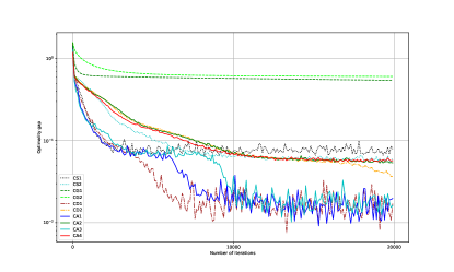
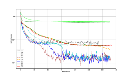
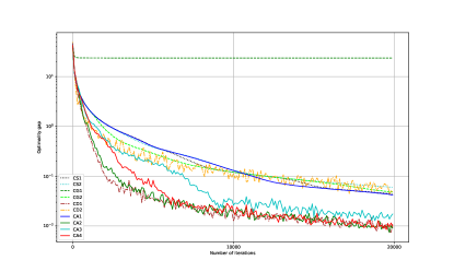
First, we compared ten algorithms (CS1)–(CA4) with constant learning rates, same as those used in the experiments on the Poincaré embeddings. Figs. 9–10 show the numerical results on the MNIST dataset, while Figs. 11–12 show the numerical results on the digits dataset. Figs. 9–10 indicate that Algorithm 1 performed well in every setting for the MNIST dataset. In particular, the behaviors of (CA2) and (CA4) are the best of all algorithms and the behavior of (CD1) is comparable to them. Moreover, Figs. 11–12 show that Algorithm 1 outperforms RSGD and RAdaGrad in every setting for the digits dataset. These figures indicate that (CD1), (CA1) and (CA3) eventually made the optimal gap the smallest. Meanwhile, Figs. 9–12 show that RAdaGrad often failed to reduce the optimal gap.

Figure 9: Optimality gap versus number of iterations in the case of constant learning rates for the MNIST dataset

Figure 10: Optimality gap versus elapsed time in the case of constant learning rates for the MNIST dataset

Figure 11: Optimality gap versus number of iterations in the case of constant learning rates for the digits dataset

Figure 12: Optimality gap versus elapsed time in the case of constant learning rates for the digitis dataset

Moreover, we examined the supervised learning performance. The classification model in this case was the Linear Support Vector Machine (Linear SVM) provided by the scikit-learn 0.23.2 package. TABLE 1 shows the 5-fold cross validation scores of the MNIST and digits dimensionally reduced by the last point generated by each algorithm with the constant learning rates. This table indicates that the algorithm which sufficiently minimizes the optimality gap also has high classification accuracy. For the MNIST dataset, since (CG1) does not converge to the optimal solution, its classification accuracy is also bad. Similarly, for the digits dataset, since (CG1) and (CG2) do not minimize the optimality gap, their classification accuracies are also bad.

Table 1: The cross validation scores of the Linear SVM in the case of constant learning rates

	MNIST	digits
CS1	0.8109	0.8658
CS2	0.8104	0.8720
CG1	0.5992	0.7929
CG2	0.8164	0.7022
CD1	0.7973	0.8736
CD2	0.8078	0.8764
CA1	0.8168	0.8764
CA2	0.8099	0.8664
CA3	0.7931	0.8520
CA4	0.8131	0.8698

4.2.2 Diminishing learning rate

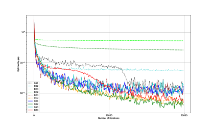
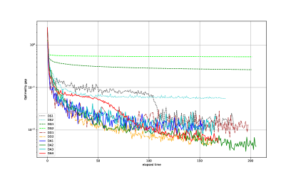
Next, we compared ten algorithms (DS1)–(DA4) with diminishing learning rates, same as those used in the experiments of the Poincaré embeddings. Figs. 13–14 show the numerical results on the MNIST dataset, while Figs. 15–16 show the numerical results on the digits dataset. Figs. 13–14 indicate that Algorithm 1 outperforms RSGD and RAdaGrad in every setting for the MNIST dataset. In particular, the behavior of (DD1) is the best of all and (DA1) performs comparably to (DD1). Moreover, Figs. 15–16 also show that Algorithm 1 outperforms RSGD and RAdaGrad in every setting for the digits dataset. In particular, the behaviors of (DA2) and (DA4) are the best of all algorithms and the behavior of (DD2) is comparable to them. Meanwhile, Figs. 13–16 show that RSGD and RAdaGrad often failed to reduce the optimal gap. Figs. 9 and 13 indicate that Algorithm 1 and RAdam with a constant learning rate are superior to the other algorithms for the MNIST dataset. Meanwhile, Figs. 11 and 15 indicate that Algorithm 1 and RAdam with a diminishing learning rate are superior to the other algorithms for the digits dataset.

Figure 13: Optimality gap versus number of iterations in the case of diminishing learning rates for the MNIST dataset

Figure 14: Optimality gap versus elapsed time in the case of diminishing learning rates for the MNIST dataset

Figure 15: Optimality gap versus number of iterations in the case of diminishing learning rates for the digits dataset

Figure 16: Optimality gap versus elapsed time in the case of diminishing learning rates for the digits dataset

As with the constant learning rate, we examined the supervised learning performance of the Linear SVM. TABLE 2 shows the 5-fold cross validation scores of the MNIST and digits dimensionally reduced by the last point generated by each algorithm with the diminishing learning rates. This table indicates that the algorithm which sufficiently minimizes the optimality gap also has high classification accuracy. Since, (DS1), (DS2), (DG1), and (DG2) for the MNIST dataset, and (DG1) and (DG2) for the digits dataset do not minimize the optimality gap, their classification accuracies are also bad.

Table 2: The cross validation scores of the Linear SVM in the case of diminishing learning rates

	MNIST	digits
DS1	0.5719	0.8709
DS2	0.6332	0.8714
DG1	0.6546	0.7145
DG2	0.5904	0.6856
DD1	0.7955	0.8670
DD2	0.7928	0.8692
DA1	0.8133	0.8759
DA2	0.7922	0.8764
DA3	0.8239	0.8842
DA4	0.8061	0.8742

5 Conclusion

This paper proposed modified RAMSGrad, a Riemannian adaptive optimization method, and presented its convergence analysis. The proposed algorithm solves the Riemannian optimization problem directly, and it can use both constant and diminishing learning rates. We applied it to Poincaré embeddings and a PCA problem. The numerical experiments showed that it converges to the optimal solution faster than RSGD and RAdaGrad, and it minimizes the objective function regardless of the initial learning rate. In particular, an experiment showed that the proposed algorithm with a constant learning rate is a good way of embedding the WordNet mammals subtree into a Poincaré subtree. Moreover, we showed that, in the PCA problem, the choice between using a constant or a diminishing learning rate depends on the dataset.

6 Acknowledgment

We are sincerely grateful to the editor and the anonymous referees for helping us improve the original manuscript.

Appendix A Lemmas

Zhang and Sra developed the following lemma in [21, Lemma 5].

Lemma A.1 (Cosine inequality in Alexandrov spaces).

Let $a,b,c$ be the sides (i.e., side lengths) of a geodesic triangle in an Alexandrov space whose curvature is bounded by $\kappa<0$ and $A$ be the angle between sides $b$ and $c$. Then,

$$a^{2}\leq\zeta{(\kappa,c)}b^{2}+c^{2}-2bc\cos{(A)},$$

where

$$\quad\zeta{(\kappa,c)}=\frac{\sqrt{|\kappa|c}}{\tanh{(\sqrt{|\kappa|c})}}.$$

We will prove the following lemma. All relations between random variables hold almost surely.

Lemma A.2.

Suppose that Assumption 2.1 (A2) holds. We define $G:=\max_{t\in\mathcal{T},x\in X}\left\lVert{\operatorname*{grad}f_{t}(x)}\right\rVert_{x}$. Let $(x_{n})_{n\in\mathbb{N}}$ and $(\hat{v}_{n})_{n\in\mathbb{N}}$ be the sequences generated by Algorithm 1. Then, for all $i\in\{1,2,\cdots,N\}$, and $k\in\mathbb{N}$,

$$~{}\left\lVert{m_{k}^{i}}\right\rVert_{x_{k}^{i}}^{2}\leq G^{2},$$ (5)

and

$$~{}\sqrt{\hat{v}_{k}^{i}}\leq G.$$ (6)

Proof.

First, we consider (5). The proof is by induction. For $k=1$, from the convexity of $\left\lVert{\cdot}\right\rVert_{x_{1}^{i}}^{2}$, we have

$$\left\lVert{m_{1}^{i}}\right\rVert_{x_{1}^{i}}^{2} \leq\left\lVert{\beta_{11}\varphi_{x_{0}^{i}\rightarrow x_{1}^{i}}^{i}(m_{0}^{i})+(1-\beta_{11})g_{t_{1}}^{i}}\right\rVert_{x_{1}^{i}}^{2}$$

$$\leq\beta_{11}\left\lVert{\varphi_{x_{0}^{i}\rightarrow x_{1}^{i}}^{i}(m_{0}^{i})}\right\rVert_{x_{1}^{i}}^{2}+(1-\beta_{11})\left\lVert{g_{t_{1}}^{i}}\right\rVert_{x_{1}^{i}}^{2}$$

$$=(1-\beta_{11})\left\lVert{g_{t_{1}}^{i}}\right\rVert_{x_{1}^{i}}^{2}$$

$$\leq\left\lVert{g_{t_{1}}^{i}}\right\rVert_{x_{1}^{i}}^{2}$$

$$\leq G^{2},$$

where we have used $0\leq\beta_{11}<1$ and $\left\lVert{g_{t_{1}}^{i}}\right\rVert_{x_{1}^{i}}\leq G$. Suppose that $\left\lVert{m_{k-1}^{i}}\right\rVert_{x_{k-1}^{i}}^{2}\leq G^{2}$. The convexity of $\left\lVert{\cdot}\right\rVert_{x_{k}^{i}}^{2}$, together with the definition of $m_{k}^{i}$, and $\left\lVert{g_{t_{k}}^{i}}\right\rVert_{x_{k}^{i}}\leq G$, guarantees that,

$$\left\lVert{m_{k}^{i}}\right\rVert_{x_{k}^{i}}^{2} \leq\beta_{1k}\left\lVert{\varphi_{x_{k-1}^{i}\rightarrow x_{k}^{i}}^{i}(m_{k-1}^{i})}\right\rVert_{x_{k}^{i}}^{2}+(1-\beta_{1k})\left\lVert{g_{t_{k}}^{i}}\right\rVert_{x_{k}^{i}}^{2}$$

$$\leq\beta_{1k}\left\lVert{m_{k-1}^{i}}\right\rVert_{x_{k-1}^{i}}^{2}+(1-\beta_{1k})G^{2}$$

$$\leq\beta_{1k}G^{2}+(1-\beta_{1k})G^{2}$$

$$=G^{2}.$$

Thus, induction ensures that, for all $k\in\mathbb{N}$,

$$\left\lVert{m_{k}^{i}}\right\rVert_{x_{k}^{i}}^{2}\leq G^{2}.$$

(6) can be proven in same way as (5). ∎

Appendix B Proof of Theorem 3.1

Proof of Theorem 3.1.

Note that

$$y_{k+1}^{i}:=\exp_{x_{k}^{i}}^{i}\left(-\alpha_{k}\dfrac{m_{k}^{i}}{\sqrt{\hat{v}_{k}^{i}}}\right).$$

Thus, we will consider a geodesic triangle consisting of three points $x_{k}^{i}$, $x_{\ast}^{i}$, and $y_{k+1}^{i}$. Let the length of each side be $a$, $b$, and $c$, respectively, such that

$$~{}\begin{cases}a:=d^{i}(y_{k+1}^{i},x_{\ast}^{i})\\ b:=d^{i}(y_{k+1}^{i},x_{k}^{i})\\ c:=d^{i}(x_{k}^{i},x_{\ast}^{i})\end{cases}.$$ (7)

It follows that

$$\cos{(\angle y_{k+1}^{i}x_{k}^{i}x_{\ast}^{i})} :=\frac{\left\langle{\log_{x_{k}^{i}}^{i}(y_{k+1}^{i}),\log_{x_{k}^{i}}^{i}(x_{\ast}^{i})}\right\rangle_{x_{k}^{i}}}{\left\lVert{\log_{x_{k}^{i}}^{i}(y_{k+1}^{i})}\right\rVert_{x_{k}^{i}}\left\lVert{\log_{x_{k}^{i}}^{i}(x_{\ast}^{i})}\right\rVert_{x_{k}^{i}}}$$

$$=\frac{\left\langle{-\alpha_{k}\dfrac{m_{k}^{i}}{\sqrt{\hat{v}_{k}^{i}}},\log_{x_{k}^{i}}^{i}(x_{\ast}^{i})}\right\rangle_{x_{k}^{i}}}{d^{i}(y_{k+1}^{i},x_{k}^{i})d^{i}(x_{k}^{i},x_{\ast}^{i})}.$$

Using Lemma A.1 with (7) and the definition of $\Pi_{X_{i}}$, we have

$$d^{i}(x_{k+1}^{i},x_{\ast}^{i})^{2}$$

$$\leq d^{i}(y_{k+1}^{i},x_{\ast}^{i})^{2}$$

$$\leq\zeta(\kappa^{i},d^{i}(x_{k}^{i},x_{\ast}^{i}))d^{i}(y_{k+1}^{i},x_{k}^{i})^{2}+d^{i}(x_{k}^{i},x_{\ast}^{i})^{2}$$

$$\quad-2d^{i}(y_{k+1}^{i},x_{k}^{i})d^{i}(x_{k}^{i},x_{\ast}^{i})\frac{\left\langle{-\alpha_{k}\dfrac{m_{k}^{i}}{\sqrt{\hat{v}_{k}^{i}}},\log_{x_{k}^{i}}^{i}(x_{\ast}^{i})}\right\rangle_{x_{k}^{i}}}{d^{i}(y_{k+1}^{i},x_{k}^{i})d^{i}(x_{k}^{i},x_{\ast}^{i})},$$

which, together with the definition of $y_{k+1}^{i}$, implies that

$$\left\langle{-m_{k}^{i},\log_{x_{k}^{i}}^{i}(x_{\ast}^{i})}\right\rangle_{x_{k}^{i}} \leq\dfrac{\sqrt{\hat{v}_{k}^{i}}}{2\alpha_{k}}(d^{i}(x_{k}^{i},x_{\ast}^{i})^{2}-d^{i}(x_{k+1}^{i},x_{\ast}^{i})^{2})$$

$$\quad+\zeta(\kappa^{i},d^{i}(x_{k}^{i},x_{\ast}^{i}))\dfrac{\alpha_{k}}{2\sqrt{\hat{v}_{k}^{i}}}\left\lVert{m_{k}^{i}}\right\rVert_{x_{k}^{i}}^{2}.$$

Plugging $m_{k}^{i}=\beta_{1k}\varphi_{x_{k-1}^{i}\rightarrow x_{k}^{i}}^{i}(m_{k-1}^{i})+(1-\beta_{1k})g_{t_{k}}^{i}$ into the above inequality and using (A1), we obtain

$$\begin{split}~{}&\left\langle{-g_{t_{k}}^{i},\log_{x_{k}^{i}}(x_{\ast}^{i})}\right\rangle_{x_{k}^{i}}\\ &\leq\dfrac{\sqrt{\hat{v}_{k}^{i}}}{2\alpha_{k}(1-\beta_{1k})}\left(d^{i}(x_{k}^{i},x_{\ast}^{i})^{2}-d^{i}(x_{k+1}^{i},x_{\ast}^{i})^{2}\right)\\ &\quad+\dfrac{\zeta(\kappa^{i},D)}{2(1-\beta_{1k})}\dfrac{\alpha_{k}}{\sqrt{\hat{v}_{k}^{i}}}\left\lVert{m_{k}^{i}}\right\rVert_{x_{k}^{i}}^{2}\\ &\quad+\frac{\beta_{1k}}{1-\beta_{1k}}\left\langle{\varphi_{x_{k-1}^{i}\rightarrow x_{k}^{i}}^{i}(m_{k-1}^{i}),\log_{x_{k}^{i}}(x_{\ast}^{i})}\right\rangle_{x_{k}^{i}}.\end{split}$$ (8)

Since (A2) implies that $f$ is geodesically convex with $g(x)=\left(g^{i}(x^{i})\right):=\operatorname*{grad}{f(x)}$, we have

$$f(x_{k})-f(x_{\ast}) \leq\left\langle{-g(x_{k}),\log_{x_{k}}(x_{\ast})}\right\rangle_{x_{k}}$$

$$=\sum_{i=1}^{N}\left\langle{-g^{i}(x_{k}^{i}),\log_{x_{k}^{i}}^{i}(x_{\ast}^{i})}\right\rangle_{x_{k}^{i}}.$$

Summing the above equality from $k=1$ to $n$, we obtain

$$~{}\frac{1}{n}\sum_{k=1}^{n}f(x_{k})-f(x_{\ast})\leq\frac{1}{n}\sum_{k=1}^{n}\sum_{i=1}^{N}\left\langle{-g^{i}(x_{k}^{i}),\log_{x_{k}^{i}}^{i}(x_{\ast}^{i})}\right\rangle_{x_{k}^{i}}.$$ (9)

Furthermore, the linearity of the Riemannian gradient ensures that

$$\mathbb{E}\left[{\left\langle{-g_{t_{k}}^{i},\log_{x_{k}^{i}}^{i}(x_{\ast}^{i})}\right\rangle_{x_{k}^{i}}}\right]$$

$$=\mathbb{E}\left[{\mathbb{E}\left[\left\langle{-g_{t_{k}}^{i},\log_{x_{k}^{i}}^{i}(x_{\ast}^{i})}\right\rangle_{x_{k}^{i}}\mathrel{}\middle|\mathrel{}t_{[k-1]}\right]}\right]$$

$$=\mathbb{E}\left[{\left\langle{-\mathbb{E}\left[g_{t_{k}}^{i}\mathrel{}\middle|\mathrel{}t_{[k-1]}\right],\log_{x_{k}^{i}}^{i}(x_{\ast}^{i})}\right\rangle_{x_{k}^{i}}}\right]$$

$$=\mathbb{E}\left[{\left\langle{-g^{i}(x_{k}^{i}),\log_{x_{k}^{i}}^{i}(x_{\ast}^{i})}\right\rangle_{x_{k}^{i}}}\right],$$

which, together with (9), implies that

$$\mathbb{E}\left[{\frac{1}{n}\sum_{k=1}^{n}f(x_{k})-f(x_{\ast})}\right]$$

$$\leq\frac{1}{n}\mathbb{E}\left[{\sum_{k=1}^{n}\sum_{i=1}^{N}\left\langle{-g^{i}(x_{k}^{i}),\log_{x_{k}^{i}}^{i}(x_{\ast}^{i})}\right\rangle_{x_{k}^{i}}}\right]$$

$$=\frac{1}{n}\mathbb{E}\left[{\sum_{k=1}^{n}\sum_{i=1}^{N}\left\langle{-g_{t_{k}}^{i},\log_{x_{k}^{i}}^{i}(x_{\ast}^{i})}\right\rangle_{x_{k}^{i}}}\right].$$

From (LABEL:eq:convexineq) and the above inequality, we have

$$\begin{split}~{}&\mathbb{E}\left[{\frac{1}{n}\sum_{k=1}^{n}f(x_{k})-f(x_{\ast})}\right]\\ &\leq\frac{1}{n}\mathbb{E}\left[{\sum_{k=1}^{n}\sum_{i=1}^{N}\dfrac{\sqrt{\hat{v}_{k}^{i}}}{2\alpha_{k}(1-\beta_{1k})}\left(d^{i}(x_{k}^{i},x_{\ast}^{i})^{2}-d^{i}(x_{k+1}^{i},x_{\ast}^{i})^{2}\right)}\right]\\ &\quad+\frac{1}{n}\mathbb{E}\left[{\sum_{k=1}^{n}\sum_{i=1}^{N}\dfrac{\zeta(\kappa^{i},D)}{2(1-\beta_{1k})}\dfrac{\alpha_{k}}{\sqrt{\hat{v}_{k}^{i}}}\left\lVert{m_{k}^{i}}\right\rVert_{x_{k}^{i}}^{2}}\right]\\ &\quad+\frac{1}{n}\mathbb{E}\left[{\sum_{k=1}^{n}\sum_{i=1}^{N}\frac{\beta_{1k}}{1-\beta_{1k}}\left\langle{\varphi_{x_{k-1}^{i}\rightarrow x_{k}^{i}}^{i}(m_{k-1}^{i}),\log_{x_{k}^{i}}(x_{\ast}^{i})}\right\rangle_{x_{k}^{i}}}\right].\end{split}$$ (10)

Here, let us consider the first term of the left-hand side of (LABEL:eq:exdif). We note that from the assumption for all $k\in\mathbb{N}$, $\alpha_{k}(1-\beta_{1k})\leq\alpha_{k-1}(1-\beta_{1,k-1})$, and $\beta_{1k}\leq\beta_{1,k-1}$,

$$\alpha_{k}(1-\beta_{1k})\leq\alpha_{k-1}(1-\beta_{1,k-1})\leq\alpha_{k-1}(1-\beta_{1k}),$$

which implies $\alpha_{k}\leq\alpha_{k-1}$. Using $\beta_{1k}\leq\beta_{11}$, $\alpha_{k}\leq\alpha_{k-1}$, $\sqrt{\hat{v}_{k}^{i}}\geq\sqrt{\hat{v}_{k-1}^{i}}$, and $\alpha_{k}(1-\beta_{1k})\leq\alpha_{k-1}(1-\beta_{1,k-1})$ for all $k\in\mathbb{N}$, together with (A1), we have that

$$\sum_{k=1}^{n}\sum_{i=1}^{N}\dfrac{\sqrt{\hat{v}_{k}^{i}}}{2\alpha_{k}(1-\beta_{1k})}(d^{i}(x_{k}^{i},x_{\ast}^{i})^{2}-d^{i}(x_{k+1}^{i},x_{\ast}^{i})^{2})$$

$$\leq\frac{1}{2(1-\beta_{11})}\sum_{i=1}^{N}\left[\sum_{k=2}^{n}\left(\dfrac{\sqrt{\hat{v}_{k}^{i}}}{\alpha_{k}}-\dfrac{\sqrt{\hat{v}_{k-1}^{i}}}{\alpha_{k-1}}\right)d^{i}(x_{k}^{i},x_{\ast}^{i})^{2}\right.$$

$$\left.\quad+\dfrac{\sqrt{\hat{v}_{1}^{i}}}{\alpha_{1}}d^{i}(x_{1}^{i},x_{\ast}^{i})^{2}\right]$$

$$\leq\frac{1}{2(1-\beta_{11})}\sum_{i=1}^{N}\left[\sum_{k=2}^{n}\left(\dfrac{\sqrt{\hat{v}_{k}^{i}}}{\alpha_{k}}-\dfrac{\sqrt{\hat{v}_{k-1}^{i}}}{\alpha_{k-1}}\right)D^{2}+\dfrac{\sqrt{\hat{v}_{1}^{i}}}{\alpha_{1}}D^{2}\right]$$

$$=\frac{D^{2}}{2(1-\beta_{11})}\sum_{i=1}^{N}\dfrac{\sqrt{\hat{v}_{n}^{i}}}{\alpha_{n}}$$

$$\leq\frac{NGD^{2}}{2\alpha_{n}(1-\beta_{11})},$$

where the last inequality is guaranteed by Lemma A.2. Namely,

$$~{}\begin{split}&\mathbb{E}\left[{\sum_{k=1}^{n}\sum_{i=1}^{N}\dfrac{\sqrt{\hat{v}_{k}^{i}}}{2\alpha_{k}(1-\beta_{1k})}(d^{i}(x_{k}^{i},x_{\ast}^{i})^{2}-d^{i}(x_{k+1}^{i},x_{\ast}^{i})^{2})}\right]\\ &\leq\dfrac{NGD^{2}}{2\alpha_{n}(1-\beta_{11})}.\end{split}$$ (11)

Next, let us consider the second term of the left-hand side of (LABEL:eq:exdif). From $\sqrt{\epsilon}\leq\sqrt{\hat{v}_{k}^{i}}$ and Lemma A.2, we have

$$\sum_{k=1}^{n}\sum_{i=1}^{N}\dfrac{\zeta(\kappa^{i},D)}{2(1-\beta_{1k})}\dfrac{\alpha_{k}}{\sqrt{\hat{v}_{k}^{i}}}\left\lVert{m_{k}^{i}}\right\rVert_{x_{k}^{i}}^{2}$$

$$\leq\dfrac{G^{2}}{2\sqrt{\epsilon}(1-\beta_{11})}\sum_{i=1}^{N}\zeta(\kappa_{i},D)\sum_{k=1}^{n}\alpha_{k}.$$

Namely,

$$~{}\begin{split}&\mathbb{E}\left[{\sum_{k=1}^{n}\sum_{i=1}^{N}\dfrac{\zeta(\kappa^{i},D)}{2(1-\beta_{1k})}\dfrac{\alpha_{k}}{\sqrt{\hat{v}_{k}^{i}}}\left\lVert{m_{k}^{i}}\right\rVert_{x_{k}^{i}}^{2}}\right]\\ &\leq\dfrac{G^{2}}{2\sqrt{\epsilon}(1-\beta_{11})}\sum_{i=1}^{N}\zeta(\kappa_{i},D)\sum_{k=1}^{n}\alpha_{k}.\end{split}$$ (12)

Now, let us consider the third term of the left-hand side of (LABEL:eq:exdif). Applying the Cauchy-Schwarz inequality to the term and using (A1) and Lemma A.2, it follows that

$$\sum_{k=1}^{n}\sum_{i=1}^{N}\frac{\beta_{1k}}{1-\beta_{1k}}\left\langle{\varphi_{x_{k-1}^{i}\rightarrow x_{k}^{i}}^{i}(m_{k-1}^{i}),\log_{x_{k}^{i}}(x_{\ast}^{i})}\right\rangle_{x_{k}^{i}}$$

$$\leq\sum_{k=1}^{n}\sum_{i=1}^{N}\frac{\beta_{1k}}{1-\beta_{1k}}\left\lVert{\varphi_{x_{k-1}^{i}\rightarrow x_{k}^{i}}^{i}(m_{k-1}^{i})}\right\rVert_{x_{k}^{i}}\left\lVert{\log_{x_{k}^{i}}(x_{\ast}^{i})}\right\rVert_{x_{k}^{i}}$$

$$\leq\frac{NGD}{1-\beta_{11}}\sum_{k=1}^{n}\beta_{1k}.$$

Namely,

$$~{}\begin{split}&\mathbb{E}\left[{\sum_{k=1}^{n}\sum_{i=1}^{N}\frac{\beta_{1k}}{1-\beta_{1k}}\left\langle{\varphi_{x_{k-1}^{i}\rightarrow x_{k}^{i}}^{i}(m_{k-1}^{i}),\log_{x_{k}^{i}}(x_{\ast}^{i})}\right\rangle_{x_{k}^{i}}}\right]\\ &\leq\frac{NGD}{1-\beta_{11}}\sum_{k=1}^{n}\beta_{1k}.\end{split}$$ (13)

Finally, together with (LABEL:eq:exdif), (11), (12), and (13), we have

$$\mathbb{E}\left[{\frac{1}{n}\sum_{k=1}^{n}f(x_{k})-f(x_{\ast})}\right]$$

$$\leq\dfrac{NGD^{2}}{2(1-\beta_{11})}\frac{1}{n\alpha_{n}}+\dfrac{G^{2}}{2\sqrt{\epsilon}(1-\beta_{11})}\sum_{i=1}^{N}\zeta(\kappa_{i},D)\frac{1}{n}\sum_{k=1}^{n}\alpha_{k}$$

$$\quad+\frac{NGD}{1-\beta_{11}}\frac{1}{n}\sum_{k=1}^{n}\beta_{1k}.$$

This complete the proof. ∎

Appendix C Proof of Corollary 3.1 and 3.2

Proof of Corollary 3.1.

The learning rates $\alpha_{n}:=\alpha$ and $\beta_{1n}:=\beta$ satisfy for all $n\in\mathbb{N}$, $\beta_{1n}\leq\beta_{1,n-1}$ and $\alpha_{n}(1-\beta_{1n})\leq\alpha_{n-1}(1-\beta_{1,n-1})$. Let us define

$$C_{1}:=\dfrac{G^{2}}{\sqrt{\epsilon}(1-\beta_{11})}\sum_{i=1}^{N}\zeta(\kappa_{i},D)>0,$$

and

$$C_{2}:=\frac{NGD}{1-\beta_{11}}.$$

Using the definitions of $C_{1}$ and $C_{2}$, (LABEL:eq:main) can be written as

$$\mathbb{E}\left[{\frac{1}{n}\sum_{k=1}^{n}f(x_{k})-f(x_{\ast})}\right]\leq\dfrac{NGD^{2}}{2\alpha(1-\beta_{11})}\frac{1}{n}+C_{1}\alpha+C_{2}\beta.$$

This complete the proof. ∎

Proof of Corollary 3.2.

Let $\alpha_{n}=1/n^{\eta}$ $(\eta\in[1/2,1))$ and $(\beta_{1n})_{n\in\mathbb{N}}$ satisfies $\beta_{1n}\leq\beta_{1,n-1}$ and $\alpha_{n}(1-\beta_{1n})\leq\alpha_{n-1}(1-\beta_{1,n-1})$ for all $n\in\mathbb{N}$, and $\sum_{k=1}^{\infty}\beta_{1k}<\infty$. First, we obviously have

$$~{}\lim_{n\to\infty}\frac{1}{n}\sum_{k=1}^{n}\beta_{1k}\leq\lim_{n\to\infty}\frac{B_{1}}{n}=0,$$ (14)

where $B_{1}:=\sum_{k=1}^{\infty}\beta_{1k}<\infty$. We have that

$$\lim_{n\to\infty}\frac{1}{n\alpha_{n}}=\lim_{n\to\infty}\frac{1}{n^{1-\eta}}=0.$$

Furthermore, we have

$$~{}\frac{1}{n}\sum_{k=1}^{n}\alpha_{k} \leq\frac{1}{n}\left(1+\int_{1}^{n}\frac{dt}{t^{\eta}}\right)\leq\frac{1}{1-\eta}\frac{1}{n^{1-\eta}}.$$ (15)

This, together with (LABEL:eq:main), (14), and (15), proves the assertion of Corollary 3.2. ∎

References

• [1] P.-A. Absil, R. Mahony, and R. Sepulchre. Optimization algorithms on matrix manifolds. Princeton University Press, 2008.
• [2] G. Bécigneul and O.-E. Ganea. Riemannian adaptive optimization methods. Proceedings of The International Conference on Learning Representations, 2019.
• [3] S. Bonnabel. Stochastic gradient descent on Riemannian manifolds. IEEE Transactions on Automatic Control, 58(9):2217–2229, 2013.
• [4] J. Duchi, E. Hazan, and Y. Singer. Adaptive subgradient methods for online learning and stochastic optimization. Journal of machine learning research, pages 2121–2159, 2011.
• [5] O.-E. Ganea, G. Bécigneul, and T. Hofmann. Hyperbolic neural networks. In Advances in neural information processing systems, pages 5345–5355, 2018.
• [6] H. Iiduka. Appropriate learning rates of adaptive learning rate optimization algorithms for training deep neural networks. arXiv preprint arXiv:2002.09647, 2020.
• [7] A. Iosifidis, A. Tefas, and I. Pitas. Graph embedded extreme learning machine. IEEE Transactions on Cybernetics, 46(1):311–324, 2015.
• [8] H. Kasai, P. Jawanpuria, and B. Mishra. Riemannian adaptive stochastic gradient algorithms on matrix manifolds. In International Conference on Machine Learning, pages 3262–3271, 2019.
• [9] D. P. Kingma and J. Ba. Adam: A method for stochastic optimization. Proceedings of The International Conference on Learning Representations, pages 1–15, 2015.
• [10] Y. LeCun, C. Cortes, and C. J. Burges. The mnist database. URL http://yann.lecun.com/exdb/mnist, 1998.
• [11] C. Li, G. López, and V. Martquez. Iterative algorithms for nonexpansive mappings on Hadamard manifolds. Taiwanese Journal of Mathematics, 14(2):541–559, 2010.
• [12] S. Mao, L. Xiong, L. Jiao, T. Feng, and S.-K. Yeung. A novel Riemannian metric based on Riemannian structure and scaling information for fixed low-rank matrix completion. IEEE Transactions on Cybernetics, 47(5):1299–1312, 2016.
• [13] M. Nickel and D. Kiela. Poincaré embeddings for learning hierarchical representations. In Advances in neural information processing systems, pages 6338–6347, 2017.
• [14] S. J. Reddi, S. Kale, and S. Kumar. On the convergence of Adam and beyond. Proceedings of The International Conference on Learning Representations, pages 1–23, 2018.
• [15] T. Sakai. Riemannian geometry, volume 149. American Mathematical Society, 1996.
• [16] H. Sato, H. Kasai, and B. Mishra. Riemannian stochastic variance reduced gradient algorithm with retraction and vector transport. SIAM Journal on Optimization, 29(2):1444–1472, 2019.
• [17] X. Shen and F.-L. Chung. Deep network embedding for graph representation learning in signed networks. IEEE Transactions on Cybernetics, 2018.
• [18] A. A. Ungar. A gyrovector space approach to hyperbolic geometry. Synthesis Lectures on Mathematics and Statistics, 1(1):1–194, 2008.
• [19] R. Walter. On the metric projection onto convex sets in riemannian spaces. Archiv der Mathematik, 25(1):91–98, 1974.
• [20] M. D. Zeiler. Adadelta: an adaptive learning rate method. arXiv preprint arXiv:1212.5701, 2012.
• [21] H. Zhang and S. Sra. First-order methods for geodesically convex optimization. In Conference on Learning Theory, pages 1617–1638, 2016.
• [22] P. Zhou, X. Yuan, S. Yan, and J. Feng. Faster first-order methods for stochastic non-convex optimization on Riemannian manifolds. IEEE transactions on Pattern Analysis and Machine Intelligence, 2019.